Article

The Hamilton–Jacobi Theory for Contact Hamiltonian Systems

1
Instituto de Ciencias Matemáticas, Consejo Superior de Investigaciones Científicas, C/Nicolás Cabrera, 13-15, 28049 Madrid, Spain
2
Real Academia de Ciencias, C/Valverde 22, 28004 Madrid, Spain
*
Author to whom correspondence should be addressed.
Mathematics 2021, 9(16), 1993; https://doi.org/10.3390/math9161993
Submission received: 5 July 2021 / Revised: 13 August 2021 / Accepted: 15 August 2021 / Published: 20 August 2021

Abstract

:
The aim of this paper is to develop a Hamilton–Jacobi theory for contact Hamiltonian systems. We find several forms for a suitable Hamilton–Jacobi equation accordingly to the Hamiltonian and the evolution vector fields for a given Hamiltonian function. We also analyze the corresponding formulation on the symplectification of the contact Hamiltonian system, and establish the relations between these two approaches. In the last section, some examples are discussed.

1. Introduction

The Hamilton–Jacobi equation is an alternative formulation of classical mechanics, equivalent to other formulations, such as Lagrangian and Hamiltonian mechanics [1,2]. The Hamilton–Jacobi equation is particularly useful in identifying conserved quantities for mechanical systems, which may be possible even when the mechanical problem itself cannot be solved completely.
The Hamilton–Jacobi equation has been extensively studied in the case of symplectic Hamiltonian systems, more specifically, for Hamiltonian functions H defined in the cotangent bundle T * Q of the configuration space Q. The Hamiltonian vector field is obtained by the equation
i X H ω Q = d H ,
where ω Q is the canonical symplectic form on T * Q . As we know, bundle coordinates ( q i , p i ) are also Darboux coordinates so that X H has the local form
X H = H p i q i H q i p i .
The Hamilton–Jacobi problem consists in finding a function S : Q R such that
H q i , S q i = E ,
for some E R . The above, Equation (1), is called the Hamilton–Jacobi equation for H. Of course, one easily see that (1) can be written as follows:
d ( H d S ) = 0 ,
which opens the possibility to consider general 1-forms on Q (considered as sections of the cotangent bundle π Q : T * Q Q ).
Recently, the observation that given such a section γ : Q T * Q permits to relate X H with its projection X H γ via γ onto Q, in the sense that X H γ and X H are γ -related if and only if (2) holds, provided that γ be closed (or, equivalently, its image be a Lagrangian submanifold of ( T * Q , ω Q ) ) has opened the possibility to discuss the Hamilton–Jacobi problem in many other scenarios [3,4,5,6]: nonholonomic systems, multisymplectic field theories, and time-dependent mechanics, among others.
In Reference [7], we have started the extension of the Hamilton–Jacobi theory for contact Hamiltonian systems (also see Reference [8]). Let us recall that a contact Hamilton system is defined by a Hamiltonian function on a contact manifold, in our case, the extended cotangent bundle T * Q × R equipped with the canonical contact form η Q = d z θ Q , where z is a global coordinate in R and θ Q the Liouville form on T * Q , with the obvious identifications.
Contact Hamiltonian systems are widely used in many fields of Physics, such as thermodynamics, dissipative systems, cosmology, and even in Biology (the so-called neurogeometry). The corresponding Hamilton equations were obtained in 1930 by G. Herglotz [9] using a variational principle that extends the usual one of Hamilton, but they can be alternatively derived using contact geometry.
The goal of this paper is to continue the study of the Hamilton–Jacobi problem in the contact context, using the two vector fields associated to the Hamiltonian H:
  • the Hamiltonian vector field:
    X H = H p i q i H q i + p i H z p i + p i H p i H z ;
  • the evolution vector field:
    E H = H p i q i H q i + p i H z p i + p i H p i z .
We notice that the Hamilton–Jacobi problem has been treated by other authors [10,11], who establish a relationship between the Herglotz variational principle and the Hamilton–Jacobi equation, although their interests are analytical rather than geometrical.
The content of the paper is as follows. Section 2 is devoted to introducing the main ingredients of contact manifolds and contact Hamiltonian systems, as well as the interpretation of a contact manifold as a Jacobi structure. In Section 3, we discuss the different types of submanifolds of a contact manifold. Section 4 is the main part of the paper; there, we discuss the Hamilton–Jacobi problem for a contact Hamiltonian vector field, as well as for the corresponding evolution vector field. The results are more involved than in the case of symplectic Hamiltonian systems due to the different possibilities that may occur. In Section 5, we study the relations of the Hamilton–Jacobi problem for a contact Hamiltonian systems and its symplectification. Finally, some examples are discussed in Section 6.

2. Contact Hamiltonian Systems

2.1. Contact Manifolds

Consider a contact manifold [12,13,14,15,16,17] ( M , η ) with contact form η ; this means that η d η n 0 , and M has odd dimension 2 n + 1 . Then, there exists a unique vector field R (called Reeb vector field) such that
i R d η = 0 , i R η = 1 .
There is a Darboux theorem for contact manifolds (see References [18,19]) so that, around each point in M, one can find local coordinates (called Darboux coordinates) ( q i , p i , z ) such that
η = d z p i d q i ,
and we have
R = z .
The contact structure defines an isomorphism between tangent vectors and covectors. For each x M ,
¯ : T x M T x * M v i v d η + η ( v ) η .
Similarly, we obtain a vector bundle isomorphism
T M T * M
over M.
We will also denote by ¯ : X ( M ) Ω 1 ( M ) the corresponding isomorphism of C ( M ) -modules between vector fields and 1-forms over M; ♯ will denote the inverse of ¯ .
Therefore, we have that
¯ ( R ) = η ,
so that, in this sense, R is the dual object of η .
For a Hamiltonian function H on M, we define the Hamiltonian vector field X H by
¯ ( X H ) = d H ( R ( H ) + H ) η .
In Darboux coordinates, we get this local expression:
X H = H p i q i H q i + p i H z p i + p i H p i H z .
Therefore, an integral curve ( q i ( t ) , p i ( t ) , z ( t ) ) of X H satisfies the contact Hamilton equations
d q i d t = H p i ,
d p i d t = H q i + p i H z ,
d z d t = p i H p i H .
In addition to the Hamiltonian vector field X H associated to a Hamiltonian function H, there is another relevant vector field, called evolution vector field defined by
E H = X H + H R ,
so that it reads in local coordinates as follows:
E H = H p i q i ( H q i + p i H z ) p i + p i H p i z .
Consequently, the integral curves of E H satisfy the differential equations
d q i d t = H p i ,
d p i d t = H q i + p i H z ,
d z d t = p i H p i .
Remark 1.
The evolution vector field plays a relevant role in the geometric description of thermodynamics (see References [20,21]).
Given a contact 2 n + 1 dimensional manifold ( M , η ) , we can consider the following distributions on M, that we will call vertical and horizontal distribution, respectively:
H = ker η , V = ker d η .
We have a Whitney sum decomposition
T M = H V ,
and, at each point x M :
T x M = H x V x .
We will denote by π H and π V the projections onto these subspaces. We notice that dim H = 2 n and dim V = 1 , and that ( d η ) | H is non-degenerate, and V is generated by the Reeb vector field R .
Definition 1.
1. 
A diffeomorphism between two contact manifolds F : ( M , η ) ( N , ξ ) is a contactomorphism if
F * ξ = η .
2. 
A diffeomorphism F : ( M , η ) ( N , ξ ) is a conformal contactomorphism if there exists a nowhere zero function f C ( M ) such that
F * ξ = f η .
3. 
A vector field X X ( M ) is an infinitesimal contactomorphism (respectively, infinitesimal conformal contactomorphism) if its flow ϕ t consists of contactomorphisms (respectively, conformal contactomorphisms).
Therefore, we have
Proposition 1.
1. 
A vector field X is an infinitesimal contactomorphism if and only if
L X η = 0 .
2. 
X is an infinitesimal conformal contactomorphism if and only if there exists g C ( M ) such that
L X η = g η .
In this case, we say that ( g , X ) is an infinitesimal conformal contactomorphism.
If ( M , η ) is a ( 2 n + 1 ) -dimensional contact manifold and takes Darboux coordinates ( q 1 , , q n , p 1 , , p n , z ) , then
V = < z > , H = < A i , B i > ,
where
A i = q i p i z , B i = p i .
{ A 1 , B 1 , , A n , B n , R } and { d q 1 , d p 1 , , d q n , d p n , η } are dual basis.
We also have
[ A i , B i ] = R .

2.2. Contact Manifolds as Jacobi Structures

Definition 2.
A Jacobi manifold [19,22,23] is a triple ( M , Λ , E ) , where Λ is a bivector field (a skew-symmetric contravariant 2-tensor field), and E X ( M ) is a vector field, so that the following identities are satisfied:
[ Λ , Λ ] = 2 E Λ , L E Λ = [ E , Λ ] = 0 ,
where [ · , · ] is the Schouten–Nijenhuis bracket.
Given a Jacobi manifold ( M , Λ , E ) , we define the Jacobi bracket:
{ · , · } : C ( M ) × C ( M ) R , ( f , g ) { f , g } ,
where
{ f , g } = Λ ( d f , d g ) + f E ( g ) g E ( f ) .
This bracket is bilinear, antisymmetric, and satisfies the Jacobi identity. Furthermore, it fulfills the weak Leibniz rule:
supp ( { f , g } ) supp ( f ) supp ( g ) .
That is, ( C ( M ) , { · , · } ) is a local Lie algebra in the sense of Kirillov.
Conversely, given a local Lie algebra ( C ( M ) , { · , · } ) , we can find a Jacobi structure on M such that the Jacobi bracket coincides with the algebra bracket.
Remark 2.
The weak Leibniz rule is equivalent to this identity:
{ f , g h } = g { f , h } + h { f , g } + g h E ( f ) .
Given a contact manifold ( M , η ) , we can define the associated Jacobi structure ( M , Λ , E ) by
Λ ( α , β ) = d η ( α , β ) , E = R ,
where = ¯ 1 . For an arbitrary function f on M, we can prove that the Hamiltonian vector field X f with respect to the contact structure η coincides with the one defined by its associated Jacobi structure, say:
X f = Λ ( d f ) f R ,
where Λ is the vector bundle morphism from tangent covectors to tangent vectors defined by Λ , i.e.,
< Λ ( α ) , β > = Λ ( α , β ) ,
for all covectors α and β .

3. Submanifolds

As in the case of symplectic manifolds, we can consider several interesting types of submanifolds of a contact manifold ( M , η ) . To define them, we will use the following notion of complement for contact structures [13]:
Let ( M , η ) be a contact manifold and x M . Let Δ x T x M be a linear subspace. We define the contact complement of Δ x
Δ x Λ = Λ ( Δ x o ) ,
where Δ x o = { α x T x * M α x ( Δ x ) = 0 } is the annihilator.
We extend this definition for distributions Δ T M by taking the complement pointwise in each tangent space.
Here, Λ is the associated 2-tensor according to the previous section.
Definition 3.
Let N M be a submanifold. We say that N is:
  • Isotropic if T N T N Λ .
  • Coisotropic if T N T N Λ .
  • Legendrian or Legendre if T N = T N Λ .
The coisotropic condition can be written in local coordinates as follows.
Let N M be a k-dimensional manifold given locally by the zero set of functions ϕ a : U R , with a { 1 , , k } .
We have that
T N λ = < Z a | a = 1 , , k > ,
where
Z a = Λ ( d ϕ a ) .
Therefore, N is coisotropic if and only if, Z a ( ϕ b ) = 0 for all a , b .
Notice that
Z a = ϕ a q i + p i ϕ a z p i + ϕ a p i q i p i z .
According to (11), we conclude that N is coisotropic if and only if
ϕ a q i + p i ϕ a z ϕ b p i + ϕ a p i ϕ b q i p i ϕ b z = 0 ,
for all a , b .
Using the above results, one can easily prove the following characterization of a Legendrian submanifold.
Proposition 2.
Let ( M , η ) be a contact manifold of dimension 2 n + 1 . A submanifold N of M is Legendrian if and only if it is a maximal integral manifold of ker η (and then it has dimension n).
Consider a function f : Q × R , and let η Q = d z ρ * θ Q the canonical contact structure on T * Q × R . Here, ρ : T * Q × R T * Q is the canonical projection, and θ Q is the canonical Liouville form on T * Q . In bundle coordinates ( q i , p i , z ) , we have
η Q = d z p i d q i ,
so that ( q i , p i , z ) are Darboux coordinates.
We denote by j 1 f : Q T * Q × R the 1-jet of f, say:
j 1 f ( q i ) = q i , f q i , f ( q i ) .
Then, one immediately checks that j 1 f ( Q ) is a Legendrian submanifold of ( T * Q × R , η Q ) . Moreover, we have:
Proposition 3.
A section γ : Q T * Q × R of the canonical projection T * Q × R Q is a Legendrian submanifold of ( T * Q × R , η Q ) if and only if γ is locally the 1-jet of a function f : Q R .
Remark 3.
The above result is the natural extension of the well-known fact that a section α of the cotangent bundle π Q : T * Q Q is a Lagrangian submanifold with respect to the canonical symplectic structure ω Q = d θ Q on T * Q if and only if α is a closed 1-form (and, hence, locally exact).

4. The Hamilton–Jacobi Equations

4.1. The Hamilton–Jacobi Equations for a Hamiltonian Vector Field

We consider the extended phase space T * Q × R , and a Hamiltonian function H : T * Q × R R (see the diagram below).
Mathematics 09 01993 i001
Recall that we have local canonical coordinates { q i , p i , z } , i = 1 , , n such that the one-form is η Q = d z ρ * θ Q , θ Q being the canonical 1-form on T * Q , can be locally expressed as follows:
η Q = d z i = 1 n p i d q i .
( T * Q × R , η ) is a contact manifold with Reeb vector field R = z .
Consider the Hamiltonian vector field X H for a given Hamiltonian function, say:
X H = Λ ( d H ) + H R .
In coordinates, it reads
X H = i = 1 n H p i q i i = 1 n p i H z + H q i p i + i = 1 n p i H p i H z .
We also have
¯ ( X H ) = d H ( R ( H ) + H ) η ,
where ♭ is the isomorphism previously defined. Moreover,
η ( X H ) = H .
Recall that ( T * Q × R , Λ , R ) is a Jacobi manifold with Λ given in the usual way (see Section 2.2). The proposed contact structure provides us with the contact Hamilton equations.
q ˙ i = H p i , p ˙ i = H q i p i H z , z ˙ = p i H p i H .
for all i = 1 , , n .
Consider γ a section of π : T * Q × R Q × R , i.e., π γ = id Q × R . We can use γ to project X H on Q × R just defining a vector field X H γ on Q × R by
X H γ = T π X H γ .
The following diagram summarizes the above construction:
Mathematics 09 01993 i002
Assume that, in local coordinates, we have
( q i , z ) γ ( q i , z ) = ( q i , γ j ( q i , z ) , z ) ,
we can compute T γ ( X H γ ) and obtain
T γ ( X H γ ) = H p i q i + H p i γ j q i + γ i H p i H γ j z p j + γ i H p i H z .
Therefore, from (15) and (19), we have that
X H γ = T γ ( X H γ )
if and only if
H q j + γ j q i H p i + γ j H z + γ i γ j z H p i H γ j z = 0 .
Assume now that:
  • γ ( Q × R ) is a coisotropic submanifold of ( T * Q × R , η Q ) ;
  • γ z ( Q ) is a Lagrangian submanifold of ( T * Q , ω Q ) , for any z R , where γ z ( q ) = ρ γ ( q , z ) .
    Notice that the above two conditions imply that γ ( Q × R ) is foliated by Lagrangian leaves γ z ( Q ) , z R .
We will discuss the consequences of the above conditions. The submanifold γ ( Q × R ) is locally defined by the functions
ϕ i = p i γ i = 0 .
Therefore, the first condition is equivalent to
γ i q j γ j γ i z γ j q i + γ i γ j z = 0 .
If, in addition, γ z ( Q ) is Lagrangian submanifold for any fixed z R , then we obtain
γ i q j γ j q i = 0 ,
and, using again (21), we get
γ j γ i z γ i γ j z = 0 .
Under the above conditions (using (22) and (23)), (20) becomes
H q j + H p i γ i q j + γ j H z + H p i γ i z H γ j z = 0 .
We can write down Equation (24) in a more friendly way. First of all, consider the following functions and 1-forms defined on Q × R :
  • γ o = H z + H p i γ i z ,
  • d ( H γ z ) = H q j + H p i γ i q j d q j ,
  • i z ( d ( γ * θ Q ) ) = γ j z d q j .
Therefore, Equation (24) is equivalent to
d ( H γ z ) + γ o ( γ * θ Q ) ( H γ ) ( i z ( d ( γ * θ Q ) ) ) = 0 .
Theorem 1.
Assume that a section γ of the projection T * Q × R Q × R is such that γ ( Q × R ) is a coisotropic submanifold of ( T * Q × R , η Q ) , and γ z ( Q ) is a Lagrangian submanifold of ( T * Q , ω Q ) , for any z R . Then, the vector fields X H and X H γ are γ-related if and only if (24) holds (equivalently, (25) holds).
Equations (24) and (25) are indistinctly referred as a Hamilton–Jacobi equation with respect to a contact structure. A section γ fulfilling the assumptions of the theorem and the Hamilton–Jacobi equation will be called a solution of the Hamilton–Jacobi problem for H.
Remark 4.
Notice that, if γ is a solution of the Hamilton–Jacobi problem for H, then X H is tangent to the coisotropic submanifold γ ( Q × R ) , but not necessarily to the Lagrangian submanifolds γ z ( Q ) , z R . This occurs when
X H ( z z 0 ) = 0 ,
for any z 0 , that is, if and only if
H γ z 0 = γ i H p i .
In such a case, we call γ a strong solution of the Hamilton–Jacobi problem.
A characterization of conditions on the submanifolds γ ( T Q × R ) , γ z ( T Q ) can be given as follows. Let α : Q × R Λ k ( T * Q ) be a z-dependent k-form on Q. Let d Q α be the exterior derivative at fixed z, that is:
d Q α ( q i , z ) = d α z ( q i ) ,
where α z = α ( · , z ) . In local coordinates, we have
d Q f = f q i d q i , d Q ( α i d q i ) = α j q i d q i d q j ,
where f : Q × R R is a function, and α = α i d q i : Q × R Λ 1 ( T * Q ) is a z-dependent 1-form.
Theorem 2.
Let γ be a section of T * Q × R over Q × R . Then, γ ( Q × R ) is a coisotropic submanifold, and γ z 0 ( T Q ) are Lagrangian submanifolds for all z 0 if and only if d Q γ = 0 and L / z γ = σ γ for some function σ : Q × R R . That is, there exists locally a function f : Q × R R such that d Q f = γ and d Q f z = σ d Q f .
Proof. 
Fix z 0 R ; then, γ z 0 ( Q ) is Lagrangian if and only if γ z 0 is closed; hence, d γ z 0 = 0 , so all γ z 0 ( Q ) are Lagrangian if and only if d Q γ = 0 . By the Poincaré Lemma, locally, γ = d Q f .
Now, also assume that γ ( Q × R ) is coisotropic. Then, Equation (23) can be written as
γ L / z γ = 0 ,
or, equivalently, that γ and L / z γ are linearly dependent.
Locally, we obtain that d Q f z = σ d Q f . □

4.1.1. Complete Solutions

Next, we shall discuss the notion of complete solutions of the Hamilton–Jacobi problem for a Hamiltonian H.
Definition 4.
A complete solution of the Hamilton–Jacobi equation for a Hamiltonian H is a diffeomorphism Φ : Q × R × R n T * Q × R such that, for any set of parameters λ R n , λ = ( λ 1 , , λ n ) , the mapping
Φ λ : Q × R T * Q × R ( q i , z ) Φ λ ( q i , z ) = Φ ( q i , z , λ )
is a solution of the Hamilton–Jacobi equation. If, in addition, any Φ λ is strong, then the complete solution is called a strong complete solution.
We have the following diagram:
Mathematics 09 01993 i003
where we define functions f i such that, for a point p T * Q × R , it is satisfied that
f i ( p ) = π i α Φ 1 ( p ) ,
and α : Q × R × R n R n is the canonical projection.
The first result is that
Im Φ λ = i = 1 n f i 1 ( λ i ) ,
where λ = ( λ 1 , , λ n ) . In other words,
Im Φ λ = { x T * Q × R | f i ( x ) = λ i , i = 1 , , n } .
Therefore, since X H is tangent to any of the submanifolds Im Φ λ , we deduce that
X H ( f i ) = 0 .
So, these functions are conserved quantities.
Moreover, we can compute
{ f i , f j } = Λ ( d f i , d f j ) f i R ( f j ) + f j R ( f i ) .
However,
Λ ( d f i , d f j ) = Λ ( d f i ) ( f j ) = 0
since ( T Im Φ λ ) = Λ ( ( T Im Φ λ ) o ) T Im Φ λ , so
{ f i , f j } = f i R ( f j ) + f j R ( f i ) .
Theorem 3.
There exists no linearly independent commuting set of first-integrals in involution (44) for a complete strong solution of the Hamilton–Jacobi equation.
Proof. 
If all the particular solutions are strong, then the Reeb vector field R will be transverse to the coisotropic submanifold Φ λ ( Q × R ) . Indeed, if R is tangent to that submanifold, we would have
R ( p i ( Φ λ ) i ) = ( Φ λ ) i z ,
where Φ λ ( q i , z ) = ( q i , ( Φ λ ) i , z ) . So, Φ λ does not depend on z; hence, it cannot be a diffeomorphism.
Therefore, if the brackets { f i , f j } vanish, then we would obtain that the functions f i cannot be linearly independent. Indeed, we should have
f i R ( f j ) = f j R ( f i ) ,
for all i , j . However, this would imply that f i and f j are linearly dependent in the case λ = ( 0 , , 0 ) .  □

4.1.2. An Alternative Approach

Instead of considering sections of π : T * Q × R Q × R as above, we could consider a section of the canonical projection π 1 : T * Q × R Q , say γ : Q T * Q × R .
In local coordinates, we have
( q i ) γ ( q i ) = ( q i , γ j ( q i ) , γ z ( q i ) ) .
We want γ to fulfill
X H γ = T γ X H γ ,
where X H γ = T π 1 X H γ . Using the local expression of X H , we have X H γ = i = 1 n H p i γ q i , and since
T γ q i = q i + j = 1 n γ j q i p j + γ z q i p j ,
Equation (32) holds if and only if:
γ i H z + H q i = j = 1 n H p j γ i q j , i = 1 , , n ,
i = 1 n γ i H p i H = i = 1 n H p i γ z q i .
Now, notice that
γ ˜ = ρ γ
is a 1-form on Q. Then, we locally have γ ˜ = γ i ( q ) d q i .
Next, we assume that γ ( Q ) is a Legendrian submanifold of ( T * Q × R , η Q ) . This implies that γ ˜ ( Q ) is a Lagrangian submanifold of ( T * Q , ω Q ) .
By Proposition 3, γ ( Q ) is a Legendrian submanifold if and only if it is locally the 1-jet of a function, namely γ = j 1 γ z , where we consider γ z as a function from Q to R . In other words, we have:
γ i = γ z q i .
If we assume that the section γ fulfills the above condition, we can see that Equation (33) becomes
H γ = 0 .
Definition 5.
Assume that a section γ such that γ ( Q ) is a Legendrian submanifold of ( T * Q × R , η Q ) and γ ˜ ( Q ) is a Lagrangian submanifold of ( T * Q , ω Q ) . Then, γ is called a solution of the Hamilton–Jacobi problem for the contact Hamiltonian H if and if Equation (36) holds.
We could discuss the existence of complete solutions in a similar manner to the case of the Hamiltonian vector field. We omit the details that are left to the reader.

4.2. The Hamilton–Jacobi Equations for the Evolution Vector Field

4.2.1. A First Approach

Assume that E H is the evolution vector field defined for a Hamiltonian function H : T * Q × R R . Then, we have
E H = H p i q i H q i + p i H z p i + p i H p i z .
Assume that γ is a section of the canonical projection π : T * Q × R Q × R , say γ : Q × R T * Q × R .
In local coordinates, we have
( q i , z ) γ ( q i ) = ( q i , γ j ( q i ) , z ) .
Therefore, we can define the projected evolution vector field
E H γ = T π E H γ .
We have that E H γ = T γ ( E H γ ) if and only if
H q j + H p i γ j q i + γ i H p i γ j z + γ j H z = 0 .
Assume now that:
  • γ ( Q × R ) is a coisotropic submanifold of ( T * Q × R , η Q ) ;
  • γ z ( Q ) is a Legendrian submanifold of ( T * Q × R , η Q ) , for any z R , where γ z ( q ) = γ ( q , z ) .
Then, a direct computation shows that (38) becomes
d ( H γ ) + γ o γ * ( θ Q ) = 0 ,
where
γ o = H z + H p i γ i z .
Theorem 4.
Assume that a section γ of the projection T * Q × R Q × R is such that γ ( Q × R ) is a coisotropic submanifold of ( T * Q × R , η Q ) , and γ z ( Q ) is a Legendrian submanifold of ( T * Q × R , η Q ) , for any z R . Then, the vector fields E H and E H γ are γ-related if and only if (39) holds.
Equation (39) is referred as a Hamilton–Jacobi equation for the evolution vector field. A section γ fulfilling the assumptions of the theorem and the Hamilton–Jacobi equation will be called a solution of the Hamilton–Jacobi problem for the evolution vector field of H.

4.2.2. An Alternative Approach

We will maintain the notations of the previous subsection, but now γ is a section of the canonical projection π 1 : T * Q × R Q , say γ : Q T * Q × R .
In local coordinates, we have
( q i ) γ ( q i ) = ( q i , γ j ( q i ) , γ z ( q i ) ) .
As in the above sections, we define the projected evolution vector field
E H γ = T π 1 E H γ .
A direct computation shows that E H γ = T γ ( E H γ ) if and only if
H q j + H p i γ j q i + γ j H z = 0 ,
H p i γ z q i γ i = 0 .
If we assume that γ = j 1 f , for some function f : Q R (or, equivalently, γ ( Q ) is a Legendrian submanifold of ( T * Q × R , η Q ) ), then
γ i = γ z q i ,
and so (40) is fulfilled, and (40) becomes
d ( H γ ) = 0 .
Remark 5.
Notice that f and γ z define (locally) the same 1-jet.
Therefore, we have the following.
Theorem 5.
Assume that a section γ of the projection T * Q × R Q is such that γ ( Q ) is a Legendrian submanifold of ( T * Q × R , η Q ) . Then, the vector fields E H and E H γ are γ-related if and only if (42) holds.
Equation (42) is referred as a Hamilton–Jacobi equation for the evolution vector field. A section γ fulfilling the assumptions of the theorem and the Hamilton–Jacobi equation will be called a solution of the Hamilton–Jacobi problem for the evolution vector field of H.

4.2.3. Complete Solutions

As in the case of the Hamiltonian vector field, we can consider complete solutions for the evolution vector field.
Definition 6.
A complete solution of the Hamilton–Jacobi equation for the evolution vector field E H of a Hamiltonian H on a contact manifold ( M , η ) is a diffeomorphism Φ : Q × R × R n T * Q × R such that, for any set of parameters λ = ( λ 0 , λ 1 , , λ n ) R × R n , the mapping
Φ λ : Q T * Q × R ( q i ) Φ λ ( q i ) = Φ ( q i , λ 0 , λ 1 , , λ n )
is a solution of the Hamilton–Jacobi equation.
For simplicity, we will use the notation ( λ α , α = 0 , 1 , , n ) .
As in the previous case, we define functions f α such that, for a point p T * Q × R , it is satisfied that:
f α ( p ) = π α Φ 1 ( p ) ,
where π α : Q × R × R n R is the canonical projection onto the α factor.
A direct computation shows that
Im Φ λ = α = 0 n f α 1 ( λ α ) .
In other words,
Im Φ λ = { x T * Q × R | f α ( x ) = λ α , α = 0 , , n } .
Therefore, since, under our hypothesis, E H is tangent to any of the submanifolds Im Φ λ , we deduce that
E H ( f α ) = 0 .
So, these functions are conserved quantities for the evolution vector field.
Moreover, we can compute
{ f α , f β } = Λ ( d f α , d f β ) f α R ( f β ) + f β R ( f α ) .
However,
Λ ( d f α , d f β ) = Λ ( d f α ) ( f β ) = 0 ,
since ( T Im Φ λ ) = T Im Φ λ , so
{ f α , f β } = f α R ( f β ) + f β R ( f α ) .
Theorem 6.
There exists no linearly independent commuting set of first-integrals in involution (44) for a complete solution of the Hamilton–Jacobi equation for the evolution vector field.
Proof. 
Since the images of the sections are Legendrian, then, they are integral submanifolds of ker η Q . So, the Reeb vector field R will be transverse to them, and, consequently, there is at least some index α 0 such that
R ( f α 0 ) 0 .
Therefore, if all the brackets { f α , f β } vanish, then we would obtain that the functions f α cannot be linearly independent. □

5. Symplectification of the Hamilton–Jacobi Equation

5.1. Homogeneous Hamiltonian Systems and Contact Systems

There is a close relationship between homogeneous symplectic and contact systems; see, for example, References [24,25]. Here, we briefly recall some facts about the symplectification of cotangent bundles.
For any manifold M, a function F : T * M R is said to be homogeneous if, for any p q T p * M , we have F ( λ p q ) = λ F ( p q ) for any λ R . In this situation, the function F can be projected to the projective bundle P ( T * M ) over M obtained by projectivization of every cotangent space. We are interested in the case that M = Q × R , with natural coordinates ( q i , z , P i , P z ) on T * ( Q × R ) . We note that this definition can be generalized to any vector bundle.
Let H ˜ be an homogeneous Hamiltonian function on T * ( Q × R ) . Locally, we have that H ˜ ( q i , z , λ P i , λ P z ) = λ H ˜ ( q i , z , P i , P z ) , for all λ R . Equivalently, one can write
H ˜ ( q i , z , P i , P z ) = P z H ( q i , P i / P z , z ) ,
for P z 0 , where H : T * Q × R R , H ( q i , p i , z ) = H ˜ ( q i , z , p i , 1 ) is well defined.
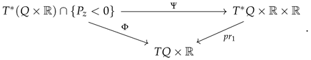
With the above changes, we have identified the manifold T * Q × R as the projective bundle P ( T * ( Q × R ) ) of the cotangent bundle T * ( Q × R ) , taking out the points at infinity, that is, the subset defined by { P z = 0 } .
Following Reference [25], Section 4.1, the map
Φ : T * ( Q × R ) { P z = 0 } T * Q × R ( q i , z , P i , P z ) ( q i , P i / P z , z ) = ( q i , p i , z )
sends the Hamiltonian symplectic system ( T * ( Q × R ) { P z = 0 } , ω Q × R , H ˜ ) onto the Hamiltonian contact system ( T * Q × R , η Q , H ) , where ω Q × R = d q i d P i + d z d P z and η Q = d z p i d q i are the canonical symplectic and contact forms, respectively. Observe that the natural coordinates of T * Q × R , denoted by ( q i , p i , z ) , correspond to the homogeneous coordinates in the projective bundle. In fact, the map Φ is projectivization up to a minus sign, i.e., the map that sends each point in the fibers of T * ( Q × R ) to the line that passes through it and the origin.
The map Φ satisfies H ¯ = P z Φ * ( H ) and ω Q = d ( P z Φ * ( η Q ) ) .
It can be shown that Φ provides a bijection between conformal contactomorphisms and homogeneous symplectomorphisms. Moreover, Φ maps homogeneous Lagrangian submanifolds L T * ( Q × R ) onto Legendrian submanifolds L = Φ ( L ) T * Q × R . Indeed, if L is homogeneous, then L is Legendrian if and only if L is Lagrangian. Moreover, the Hamilton equations for H ˜ are transformed into the Hamilton equations for H, i.e., Φ * X H ˜ = X H . See References [25,26] for more details on this topic.
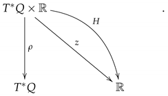
We also remark that this construction is symplectomorphic to the symplectification defined in Reference [24], which is given by
( T * Q × R × R , ω = e t ( d η Q + η Q d t ) = d ( e t η Q ) ) ,
where t is the (global) coordinate of the second R factor. The “symplectified” Hamiltonian is H ˜ = e t H so that both dynamics are p r 1 -related. That is, H ˜ is such that
( p r 1 ) * X H ˜ = X H ,
where p r 1 : T * Q × R × R T * Q × R is the projection onto the first two factors.
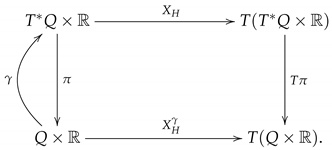
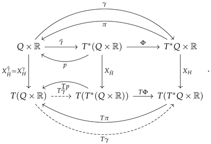
The following map provides the symplectomorphism
Ψ : T * ( Q × R ) { P z < 0 } T * Q × R × R ( q i , z , P i , P z ) ( q i , P i / P z , z , log ( P z ) ) = ( q i , p i , z ) ,
that is, Ψ = ( Φ , log ( P z ) . This map is a symplectomorphism that maps H ¯ onto H ¯ . Moreover, it is a fiber bundle automorphism over T Q × R (see the diagram below):
Mathematics 09 01993 i004

5.2. Relations for the Hamiltonian Vector Field

Now, we will establish a relationship between solutions to the Hamilton–Jacobi problem in both scenarios. Suppose that
γ ˜ : Q × R T * ( Q × R ) ( q i , z ) ( q i , γ ˜ j ( q i , z ) , z , γ ˜ t ( q i , z ) )
is a solution of the symplectic Hamilton–Jacobi equation, i.e., γ ˜ ( Q × R ) is Lagrangian and
d ( H ˜ γ ˜ ) = 0 ,
or, equivalently
T γ ˜ X H ˜ γ ˜ = X H ˜ γ ˜ ,
where X H ˜ γ ˜ = T p X H ˜ γ ˜ is the projected vector field and p : T * ( Q × R ) Q × R the canonical projection. We want to use the solution γ ˜ 
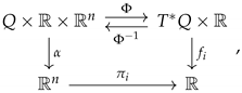
of the Hamilton–Jacobi problem in the symplectification (which we will often refer to as “symplectic solution”) to obtain a section that is a solution in the contact setting (“contact solution”, for simplicity). We assume γ ˜ t ( q i , z ) 0 and take γ = Φ γ ˜ : Q × R T * Q × R . In local coordinates:
γ : Q × R T * Q × R ( q i , z ) q i , γ j ( q i , z ) = γ ˜ j ( q i , z ) γ ˜ t ( q i , z ) , z .
We can summarize the situation in the following commutative diagram:
Mathematics 09 01993 i005
We note that the projected vector fields X H ˜ γ ˜ and X H γ coincide. The dashed lines of T γ ˜ (respectively, T γ ) commute if and only if γ ˜ is a symplectic solution (respectively, γ is a contact solution) of the Hamilton–Jacobi problem.
Lemma 1.
Let H be a Hamiltonian and H ˜ its symplectified version. Assume γ ˜ t ( q i , z ) 0 . Then, γ ˜ is a symplectic solution, or, equivalently, X H ˜ γ ˜ and X H ˜ are γ ˜ -related if and only if X H γ and X H are γ-related.
Proof. 
Assume that X H ˜ γ ˜ and X H ˜ are γ ˜ -related. Then, by the commutativity of the diagram (51), we see that X H γ and X H are γ -related.
Conversely, assume that X H γ and X H are γ -related. Let P z R { 0 } , and let
ξ : T * Q × R T * ( Q × R ) ( q i , P i , z ) ( q i , z , P i γ ˜ t ( q i , z ) ) .
We note that ξ P is the inverse of Φ along the submanifold { P z = γ t } T * ( Q × R ) . In particular, γ ˜ = ξ γ . Looking at the diagram (51), this implies that X H ˜ γ ˜ and X H ˜ are γ ˜ -related.  □
Lemma 2.
Assume that the image of γ ˜ = ( γ ˜ Q , γ ˜ t ) is Lagrangian. Then, the image of γ is coisotropic, and the images of γ z 0 are Lagrangian if and only if d Q γ Q ˜ = τ γ Q for some function τ : Q × R R .
Conversely, if the image of γ is coisotropic and the images of γ z 0 are Lagrangian, then we can choose γ t ˜ so that the image of γ ˜ is coisotropic. Indeed, it is given by either γ ˜ t = ± exp ( g ) , where g is a solution to the PDE
d Q g + γ L / z g = L / z γ .
Proof. 
Let γ ˜ = ( γ ˜ Q , γ ˜ t ) be such that its image is Lagrangian. That is, d γ ˜ = 0 . Splitting the part in Q and in R , we see that this is equivalent to
L / z γ ˜ Q = d Q γ ˜ t , d Q γ ˜ Q = 0 .
Now, γ = γ ˜ Q / γ ˜ t . By Theorem 2, it is necessary that d Q γ = 0 and ( L / z γ ) γ = 0 . We compute
d Q γ = ( d Q γ ˜ t ) γ ˜ Q γ ˜ t 2 = ( L / z γ ˜ Q ) γ ˜ Q γ ˜ t 2 =
( L / z γ ) γ = ( L / z γ ˜ t ) γ ˜ Q ( L / z γ ˜ Q ) γ ˜ t γ ˜ t 2 γ Q ˜ γ ˜ t = ( L / z γ ˜ Q ) γ ˜ Q γ ˜ t 2 ;
hence, the images of γ z 0 are Lagrangian, and the image of γ is coisotropic if and only if L / z ( γ ˜ Q ) is proportional to γ ˜ Q .
Conversely, assume that γ satisfies d Q γ = 0 and L / z γ = σ γ . We must find γ ˜ t so that (54) are satisfied. Since γ ˜ Q = γ ˜ t γ , we have that (54) are equivalent to
L / z ( γ ˜ Q ) = ( L / z γ ˜ t + σ γ ˜ t ) γ = d Q γ ˜ t ,
d Q ( γ Q ) = d Q γ ˜ t γ = 0 .
A solution for γ ˜ t on the first equation above clearly solves the second one. Since we look for nonvanishing γ ˜ t , we let g = log | γ ˜ t | so that is just
d Q g + γ L / z g = σ γ = L / z γ ,
and, if we let
A i = q i + γ i z ,
this equation can be written as
A i ( g ) = γ i z ,
and we note that this vector fields commute, indeed,
[ X i , X j ] = γ i γ j z γ j γ i z = σ γ i γ j σ γ j γ i = 0 .
If this PDE has local solutions, operating with the equations above, one has,
A i ( γ j z ) A j ( γ i z ) = 0 .
This condition is clearly necessary, and it is also sufficient by (Thm. 19.27) [27]. We have that
A i ( γ j z ) A j ( γ i z ) = γ i 2 γ j ( z ) 2 γ j 2 γ i ( z ) 2 = γ i ( σ γ j ) z γ j ( σ γ i ) z = 0 .
 □
Combining the last two results, we obtain a correspondence between symplectic and contact solutions to the Hamilton–Jacobi problem.
Theorem 7.
Let H be a Hamiltonian, and H ˜ its symplectified version. Then, γ ˜ : Q × R T * ( Q × R ) is a solution of the symplectic Hamilton–Jacobi problem for H ˜ , if and only if γ = Φ γ ˜ : Q × R T * Q × R is a solution of the contact Hamilton–Jacobi problem for H and d Q γ ˜ Q = τ γ Q for some function τ : Q × R R .
Conversely, given a contact solution γ of the Hamilton–Jacobi equation, there exists a symplectic solutions γ ˜ such that | γ ˜ | = exp ( g ) , where g is a solution to the PDE
d Q g + γ L / z g = L / z γ .

The Alternative Approach

For each z, we have sections γ = p r 2 γ ˜ z : Q T * Q × R of the form ( q i ) ( q i , γ ˜ j ( q i , z ) , γ ˜ t ( q i , z ) ) , being p r 2 : ( q i , p i , z , t ) ( q i , p i , t ) . We know that γ is a solution of the contact Hamilton–Jacobi problem if and only if γ ( Q ) is Legendrian, and
H γ = 0 .
The condition that γ ( Q ) is Legendrian is equivalent to
γ i = γ z q i ,
where we write γ ( q i ) = ( q i , γ j ( q i ) , γ z ( q i ) ) , which, by definition of γ and using that γ ( Q × R ) is Lagrangian, reads
γ ˜ i = γ ˜ t q i = γ ˜ i z ;
therefore, γ ˜ i = e z g ( q i ) , with g i functions depending only on the ( q i ) . This can be summarized as follows:
Theorem 8.
Suppose γ ˜ : Q × R T * ( Q × R ) is a solution of the symplectified Hamilton–Jacobi problem. Then,
γ : Q T * Q × R , ( q i ) ( q i , γ ˜ j ( q i , z ) , γ ˜ t ( q i , z ) )
is a solution of the contact Hamilton–Jacobi problem if and only if
H γ = 0 a n d γ ˜ i = e z g i .

5.3. Relations for the Evolution Vector Field

We now consider the evolution field E H . First, note that
T p r 1 X H ˜ = ( E H H R ) p r 1 ,
so that we cannot simply expect to project the vector field as before. In fact, one can easily prove that, under the assumption that the symplectified Hamiltonian is of the form
H ˜ = F ( t , H ) ,
then the associated vector field X H ˜ such that i X H ˜ ω = d H will never verify
T p r 1 X H ˜ = E H p r 1 .
We will now see that, despite this apparent obstruction, one can still establish some relations. Let γ ˜ : Q × R T * ( Q × R ) be a solution of the symplectified problem and define the section γ = p r 2 γ ˜ z : Q T * Q × R . This will be a solution of the associated Hamilton–Jacobi problem for the evolution field if and only if γ ( Q ) is Legendrian, and
d ( H γ ) = 0 .
The Legendrian condition is equivalent to
γ i = γ t q i ,
or, using that γ ˜ ( Q × R ) is Lagrangian, such as in the previous section,
γ ˜ i = e z g i ( q i ) .
On the other hand, we know that γ ˜ is a solution of the symplectic problem, and, therefore, d ( H ˜ γ ˜ ) = 0 , which, by definition, means
e γ ˜ t ( q i , z ) H ( q i , γ ˜ j ( q i , z ) , z ) = C
with C constant. Since γ ( q i ) = ( q i , γ ˜ j ( q i , z ) , γ ˜ t ( q i , z ) ), using the previous equation, we obtain:
H γ = C e γ ˜ t ( . γ ˜ t ( , z ) ) .
Then, the condition d ( H γ ) = 0 reads
( H γ ) γ ˜ t q i + γ ˜ t z γ ˜ t q i = 0 ,
which occurs if and only if, at every point ( q i ) , we have:
H γ = 0 or γ ˜ t q i = 0 or γ ˜ t z = 1 .
The functional form found for H γ tells us that it is either non-zero at every point or it vanishes everywhere. If it does not vanish (everywhere), we claim that the second equation must be true. Indeed, suppose the first two equations do not hold. Then, the third equation must be true not just at a given point but in an open neighborhood, and we would have
γ ˜ t = z + h ( q i ) ,
where h i are arbitrary functions. Using, again, that γ ˜ ( Q × R ) is Lagrangian, we could write
γ ˜ t q i = h q i = e z g i ( q i ) = γ ˜ i z ,
which would imply that h depends also on z. Therefore, if H γ 0 , then the second equation is true at every point. Using that γ ˜ ( Q × R ) is Lagrangian, we see this is equivalent to γ ˜ i = 0 . Therefore, we find:
Theorem 9.
Let γ ˜ : Q × R T * ( Q × R ) be a solution of the symplectified problem with γ ˜ i = e z g i , where g i : Q R , and consider the section
γ : Q T * Q × R , ( q i ) ( q i , γ ˜ j ( q i , z ) , γ ˜ t ( q i , z ) ) .
Then, γ is a solution of the contact problem for the evolution field if and only if one of the two following conditions is fulfilled:
1. 
H γ = 0 ,
2. 
γ ˜ i = 0 .

6. Examples

6.1. Particle with Linear Dissipation

Consider the Hamiltonian H:
H ( q , p , z ) = p 2 2 m + V ( q ) + λ z ,
where λ R is a constant. The extended phase space is T * Q × R R 3 .
The Hamiltonian and evolution vector field are given by
X H = p m q V q + λ z p + p 2 2 m V ( q ) λ z z ,
E H = p m q V q + λ z p + p 2 m z .
Assume that γ : Q T * Q × R is a section of the canonical projection T * Q × R Q , that is,
γ ( q ) = ( q , γ p ( q ) , γ z ( q ) ) .
We assume that γ ( Q ) is a Legendrian submanifold of T * Q × R as in Section 4.2.2; then,
γ p ( q ) = d γ z d q ,
and E H and E H γ are γ -related if and only if
H γ = k ,
for a constant k R . Then, the Hamilton–Jacobi equation becomes
H ( γ ( q ) ) = γ p 2 2 m + V ( q ) + λ γ z = k ,
or, equivalently,
d γ z d q 2 2 m + V ( q ) + λ γ z = k ,
which is a non-linear ordinary differential equation.

6.2. Application to Thermodynamic Systems

We consider thermodynamic systems in the so-called energy representation. Hence, the thermodynamic phase space, representing the extensive variables, is the manifold T * Q × R , equipped with its canonical contact form
η Q = d U p i d q i .
The local coordinates on the configuration manifold Q are ( q i , U ) , where U is the internal energy, and q i ’s denote the rest of extensive variables. Other variables, such as the entropy, may be chosen instead of the internal energy, by means of a Legendre transformation.
The state of a thermodynamic system always lies on the equilibrium submanifold L T * Q × R , which is a Legendrian submanifold. The pair ( T * Q × R , L ) is a thermodynamic system. The equations (locally) defining L are called the state equations of the system.
On a thermodynamic system ( T * Q × R , L ) , one can consider the dynamics generated by a Hamiltonian vector field X H associated to a Hamiltonian H. If this dynamics represents quasistatic processes, meaning that, at every time the system is in equilibrium, that is, its evolution states remain in the submanifold L , it is required for the contact Hamiltonian vector field X H to be tangent to L . This happens if and only if H vanishes on L .
Using Hamilton–Jacobi theory, one sees that a section γ satisfied H γ = 0 if and only if X H γ and X H are γ -related.

The Classical Ideal Gas

A detailed description of this example can be found in References [28,29]; we summarize here the main ingredients.
The classical ideal gas is described by the following variables.
  • U: internal energy,
  • T: temperature,
  • S: entropy,
  • P: pressure,
  • V: volume,
  • μ : chemical potential,
  • N: mole number.
Thus, the thermodynamic phase space is T * R 3 × R , and the contact 1-form is
η = d U T d S + P d V μ d N .
The Hamiltonian function is
H = T S R N T + μ N U ,
where R is the constant of ideal gases. The Reeb vector field is R = U .
The Hamiltonian and evolution vector fields are just
X H = ( S R N ) S + N N + P P + R T μ + U U ,
E H = ( S R N ) S + N N + P P + R T μ + ( T S R N T + μ N ) U .
The Hamiltonian vector field here represents an isochoric and isothermal process on the ideal gas.
Assume that γ : R 3 T * R 3 × R is the section locally given by
γ ( S , V , N ) = ( S , V , N , γ T , γ P , γ μ γ U ) ;
we know that γ ( R 3 ) is a Legendrian submanifold of ( T * R 3 × R , η ) if and only if,
γ T = γ U S , γ P = γ U V , γ μ = γ U N .
The Hamilton–Jacobi equation is
( H γ ) ( S , V , N ) = ( S R N ) γ T + N γ μ γ U = k ,
for some k R . That is,
( H γ ) ( S , V , N ) = ( S R N ) γ U S + N γ U N γ U = k .
This is a first order linear PDE, whose solution is given by
γ U ( S , V , N ) = k arcsinh S S 2 + 7 N + S 2 + F ( S 2 + ( R N S ) 2 , V ) ,
with F : R 2 R an arbitrary function. The case k = 0 , which is the one relevant for the thermodynamic interpretation, is given by
γ U ( S , V , N ) = F ( S 2 + ( R N S ) 2 , V ) .

7. Conclusions

In this paper, we construct a Hamilton–Jacobi theory for contact Hamiltonian systems, which completes, in several respects, some first approximations in previous papers. Let us consider the two main vector fields associated with a given Hamiltonian, which give rise to two distinct dynamics. On the one hand, the usual Hamiltonian vector field, X H , and, on the other hand, the so-called evolution field, E H . The latter plays an essential role in the study of thermodynamic systems. For both cases, the corresponding Hamilton–Jacobi equations are obtained (two for each dynamics, four in total), characterizing them with the characteristics that their solutions provide coisotropic, Lagrangian, or Legendrian submanifolds. These characterizations have allowed in the case of symplectic mechanics to obtain new results in the study of the properties of the Hamilton–Jacobi equation.
We also study an alternative formulation, using the so-called symplectification of a contact structure, thus relating our results to those known in that case, although the problem we encounter is that we must deal with homogeneous Hamiltonians (which does not occur in a contact context). Finally, we consider two examples to illustrate the results obtained.
We are confident that these results can be applied in different areas, such as cosmology or thermodynamics, to name just a few. Among the tasks we intend to address is the detailed study of the discrete Hamilton–Jacobi equation and the identification of generating functions that allow us to use the general theory to integrate the dissipative equations generated by the Hamiltonian.

Author Contributions

All authors have contributed equally. All authors have read and agreed to the published version of the manuscript.

Funding

We acknowledge the financial support from the MINECO Grant PID2019- 106715GB-C21. Manuel Laínz wishes to thank MICINN and ICMAT for a FPI-Severo Ochoa predoctoral contract PRE2018-083203. Álvaro Muñiz thanks ICMAT for the “Grant Programme Severo Ochoa–ICMAT: Introduction to Research 2020” and Fundación Barrié for its fellowship for postgraduate studies.

Institutional Review Board Statement

Not applicable.

Informed Consent Statement

Not applicable.

Data Availability Statement

Not applicable.

Acknowledgments

We thank the referees for their constructive input.

Conflicts of Interest

The authors declare no conflict of interest.

References

  1. Abraham, R.; Marsden, J.E. Foundations of Mechanics; Benjamin/Cummings Publishing Company: Reading, MA, USA, 1978; Volume 36. [Google Scholar]
  2. Arnold, V.I. Mathematical Methods of Classical Mechanics, 2nd ed.; Graduate Texts in Mathematics 60; Springer: New York, NY, USA, 1997. [Google Scholar]
  3. Barbero-Liñán, M.; de León, M.; Diego, D.M.D. Lagrangian submanifolds and the Hamilton–Jacobi equation. Monatsh. Math. 2013, 170, 381–404. [Google Scholar] [CrossRef] [Green Version]
  4. de León, M.; Diego, D.M.D.; Vaquero, M. Hamilton-Jacobi theory on Poisson manifolds. J. Geom. Mech. 2014, 6, 121–140. [Google Scholar] [CrossRef]
  5. de León, M.; Diego, D.M.D.; Vaquero, M. Hamilton–Jacobi theory, symmetries and coisotropic reduction. J. Math. Pures Appl. 2017, 107, 591–614. [Google Scholar] [CrossRef] [Green Version]
  6. Grillo, S.; Padrón, E. Extended Hamilton–Jacobi theory, contact manifolds, and integrability by quadratures. J. Math. Phys. 2020, 61, 012901. [Google Scholar] [CrossRef] [Green Version]
  7. de León, M.; Sardón, C. Cosymplectic and contact structures for time-dependent and dissipative Hamiltonian systems. J. Phys. Math. Theor. 2017, 50, 255205. [Google Scholar] [CrossRef] [Green Version]
  8. de León, M.; Lainz-Valcázar, M. A review on contact Hamiltonian and Lagrangian systems. Rev. Acad. Canaria Cienc. 2019, XXXI, 1–46. [Google Scholar]
  9. Herglotz, G. Beruhrungstransformationen; Lectures at the University of Gottingen; University of Gottingen: Göttingen, Germany, 1930. [Google Scholar]
  10. Cannarsa, P.; Cheng, W.; Jin, L.; Wang, K.; Yan, J. Herglotz’ variational principle and Lax-Oleinik evolution. J. Math. Pures Appl. 2020, 141, 99–136. [Google Scholar] [CrossRef]
  11. Jin, L.; Zhang, J.; Zhao, K. Smooth subsolutions of the discounted Hamilton-Jacobi equations. arXiv 2020, arXiv:2007.10687. [Google Scholar]
  12. Bravetti, A. Contact Hamiltonian Dynamics: The Concept and Its Use. Entropy 2017, 195, 35. [Google Scholar] [CrossRef]
  13. de León, M.; Lainz–Valcázar, M. Contact Hamiltonian systems. J. Math. Phys. 2020, 153, 103651. [Google Scholar] [CrossRef]
  14. de León, M.; Rodrigues, P.R. Methods of Differential Geometry in Analytical Mechanics; Elsevier: Amsterdam, The Netherland, 2011; Volume 158. [Google Scholar]
  15. Albert, C. Le théorème de réduction de Marsden-Weinstein en géométrie cosymplectique et de contact. J. Geom. Phys. 1989, 6, 627–649. [Google Scholar] [CrossRef]
  16. Bravetti, A.; de León, M.; Marrero, J.C.; Padrón, E. Invariant measures for contact Hamiltonian systems: Symplectic sandwiches with contact bread. J. Phys. Math. Theor. 2020, 53, 455205. [Google Scholar] [CrossRef]
  17. de León, M.; Lainz–Valcázar, M. Infinitesimal symmetries in contact Hamiltonian systems. J. Geom. Phys. 2020, 153, 103651. [Google Scholar] [CrossRef] [Green Version]
  18. Godbillon, C. Géométrie Différentielle et Mécanique Analytique; Hermann: Paris, France, 1969. [Google Scholar]
  19. Libermann, P.; Marle, C.M. Symplectic Geometry and Analytical Mechanics; Mathematics and Its Applications, 35; D. Reidel Publishing Co.: Dordrecht, The Netherlands, 1987; p. xvi+526. ISBN 90-277-2438-5. [Google Scholar]
  20. Simoes, A.A.; de León, M.; Lainz–Valcázar, M.; Diego, D.M.D. Contact geometry for simple thermodynamical systems with friction. Proc. R. Soc. A. 2020, 476, 16. [Google Scholar] [CrossRef]
  21. Simoes, A.A.; de Diego, D.M.; Valcázar, M.L.; de León, M. The Geometry of Some Thermodynamic Systems. In Geometric Structures of Statistical Physics, Information Geometry, and Learning; Barbaresco, F., Nielsen, F., Eds.; Springer Proceedings in Mathematics & Statistics; Springer: Cham, The Netherland, 2021; Volume 361. [Google Scholar]
  22. Kirillov, A.A. Local Lie algebras. Akad. Nauk. Sssr Mosk. Mat. Obs. Uspekhi Mat. Nauk. 1976, 31, 57–76. [Google Scholar] [CrossRef]
  23. Lichnerowicz, A. Les variétés de Jacobi et leurs algèbres de Lie associées. J. Math. Pures Appl. 1978, 57, 453–488. [Google Scholar]
  24. Ibáñez, R.; de León, M.; Marrero, J.C.; Diego, D.M.D. Co-isotropic and Legendre-Lagrangian submanifolds and conformal Jacobi morphisms. J. Phys. Math. Gen. 1997, 30, 5427. [Google Scholar] [CrossRef] [Green Version]
  25. Van der Schaft, A.; Maschke, B. Geometry of Thermodynamic Processes. Entropy 2017, 20, 925. [Google Scholar] [CrossRef] [PubMed] [Green Version]
  26. der Schaft, A.V. Liouville geometry of classical thermodynamics. arXiv 2021, arXiv:2102.05493. [Google Scholar]
  27. Lee, J.M. Introduction to Smooth Manifolds; Springer: New York, NY, USA, 2013. [Google Scholar]
  28. Ghosh, A.; Bhamidipati, C. Contact geometry and thermodynamics of black holes in AdS spacetimes. Phys. Rev. D 2019, 100, 126020. [Google Scholar] [CrossRef] [Green Version]
  29. Dereli, T.; Unluturky, K.I. Hamilton-Jacobi Formulation of the Thermodynamics of Einstein-Born-Infeld-AdS Black Holes. EPL Europhys. Lett. 2019, 125, 10005. [Google Scholar] [CrossRef] [Green Version]
Publisher’s Note: MDPI stays neutral with regard to jurisdictional claims in published maps and institutional affiliations.

