Stable Identification of Sources Located on Interface of Nonhomogeneous Media

Abstract

This paper presents a stable method for the identification of sources located on the separation interface of two homogeneous media (where one of them is contained by the other one), from measurement yielded by those sources on the exterior boundary of the media. This is an ill-posed problem because numerical instability is presented, i.e., minimal errors in the measurement can result in significant changes in the solution. To obtain the proposed stable method the identification problem is categorized into three subproblems, two of which present numerical instability and regularization methods must be applied to obtain their solution in a stable form. To manage the numerical instability due to the ill-posedness of these subproblems, the Tikhonov regularization and sequential smoothing methods are used. We illustrate this methodology in a circular and irregular region to demonstrate the feasibility of the proposed method, which yields convergent and stable solutions for input data with and without noise.

1. Introduction

Source identification problems are widely investigated in many research fields [1,2,3,4,5,6,7,8,9], and they are modeled by boundary value problems for which the analysis of the associated forward problem and its corresponding inverse problem must be considered, see, e.g., [10,11]. The latter problem involves determining the source that yields the measurement on the boundary of the region [12,13,14]. The inverse source problem appears in different applications, such as inverse electroencephalography, inverse electrocardiography and inverse geophysics (see, e.g., [15,16,17,18,19,20,21,22,23]), where the problems are modeled using differential equations. Numerical solutions to differential equations are crucial in mathematics and engineering because they appear in many applications, such as population growth, diffusion processes, electromagnetic problems, and elasticity problems. The finite difference method, the finite element method, the boundary element method, and the method of fundamental solutions are used for the numerical solution to boundary value problems, with or without initial conditions on the boundary, governed by certain partial differential equations [24,25,26,27]. The finite element method is one of the most important numerical methods for solving differential equations [28]. It has been used for solving the inverse source problem using the gradient conjugate method and a control approach [19,29,30]. Recently, it has been used to solve differential equations with the Henstock–Kurzweil functions [31]. It is applied to obtain a solution with highly oscillatory functions. Special quadratures have been applied to calculate the integrals that appear in the weak formulation of the finite element method [32]. In this study, we applied the trapezoidal rule to calculate integrals that appear in the applications of the finite element method. The layer potential technique has been used to obtain the solution to the inverse source problem in electrocardiography and electroencephalography (see [15,17,18]), and it was not considered in this study.

In this study, we investigate a case in which the sources are located on the separation interface between two different homogeneous media. The problem of identifying either sources having compact support within a finite number of small subdomains (see [12]), pointwise sources, electrostatic mono and dipole sources, or combinations of these (see [13,14]), are not considered in this work. The sources are identified from measurements on the exterior boundary of the bounded domain, and the relationship between the sources and the measurements is established using an elliptic model, as shown in Section 2. The inverse source problem associated with this elliptic model can be categorized into three problems:

• The Cauchy problem for the Laplace equation in the homogeneous annular region.
• The Dirichlet problem for the Laplace equation in the homogeneous interior region.
• The source identification problem from the normal derivatives of the solutions to the Cauchy and Dirichlet problems.

The Cauchy problem is ill-posed because it presents numerical instability, i.e., minimal errors in the measurement can yield significant changes in the solution. To manage such instability, we employed the algorithm proposed in [29], where a penalization method was applied (equivalent to the Tikhonov regularization [33,34]); the conjugate gradient method; and the finite element method, where the regularization parameter was determined by the Tikhonov criterion. To obtain the numerical solution to the forward problem and elliptical problems that appear in the conjugate gradient algorithm and the Dirichlet problem, we performed a finite element approximation [35].

The source was recovered from the normal derivatives of the solutions to the Cauchy and Dirichlet problems. For the stable recovery of the normal derivatives, we applied the sequential smoothing method.

Furthermore, we considered cases involving sources that are typically associated with applications (see [15,17]).

This paper is organized as follows. In Section 2, we introduce an elliptic model (a boundary value problem) that relates the sources with the measurements, and the results of existence and uniqueness are included for the classical and weak solutions to the given model. In Section 3, the inverse source problem is uncoupled into three problems that allow us to obtain the stable algorithm. In Section 4, we present the control approach of the Cauchy problem, cost function, and Tikhonov regularization. In Section 5, we present the analytical solution to forward and inverse problems in a circular domain using circular harmonics expansion series. In Section 6, we present the stable algorithm for the inverse source problem. Section 7 presents the numerical results of the proposed method for circular and irregular geometries. In Section 8, we present a discussion about the most relevant results obtained in this work. Finally, conclusions are provided in Section 9.

2. Mathematical Model

2.1. Elliptic Model

In this study, we focus on the following boundary value problem: Find $u_1$ and $u_2$ such that

$$\begin{array}{ccc}\hfill \Delta u_1=0,& & \mathrm{in}{\mathsf{\Omega }}_1,\hfill \end{array}$$

(1)

$$\begin{array}{ccc}\hfill \Delta u_2=0,& & \mathrm{in}{\mathsf{\Omega }}_2,\hfill \end{array}$$

(2)

$$\begin{array}{ccc}\hfill u_1=u_2,& & \mathrm{on}{S}_1,\hfill \end{array}$$

(3)

$$\begin{array}{ccc}\hfill {\sigma }_1\frac{\partial u_1}{\partial n_1}={\sigma }_2\frac{\partial u_2}{\partial n_1}+g,& & \mathrm{on}{S}_1,\hfill \end{array}$$

(4)

$$\begin{array}{ccc}\hfill \frac{\partial u_2}{\partial n_2}=0,& & \mathrm{on}{S}_2,\hfill \end{array}$$

(5)

where $\mathsf{\Omega }={\overline{\mathsf{\Omega }}}_1\cup {\mathsf{\Omega }}_2\subset {\mathbb{R}}^n$, with $n=2$ or 3, is a sufficiently smooth region. The positive constants ${\sigma }_1$ and ${\sigma }_2$ are the conductivities of regions ${\mathsf{\Omega }}_1$ and ${\mathsf{\Omega }}_2$, respectively (see Figure 1). Function g represents the source defined on the interface $S_1$, $n_1$ and $n_2$ are the unit outward normal vectors on the boundaries of ${\mathsf{\Omega }}_1$ and ${\mathsf{\Omega }}_2$, respectively. We denote u as the solution to problem (1)–(5) in $\mathsf{\Omega }$ and $u_i={\left.u\right|}_{{\mathsf{\Omega }}_i}$, $i=1,2$. $\Delta$ represents the Laplace operator, which is also denoted by ${\nabla }^2$. Boundary condition (3) corresponds to the continuity of the potential, and condition (4) corresponds to the jump of the normal flux, which is equal to function g. Condition (5) indicates that the conductivity in the exterior region ${\mathbb{R}}^n\backslash \overline{\mathsf{\Omega }}$ is zero (in some applications, it corresponds to the conductivity of the air).

From Green’s formulas, the following compatibility condition was obtained:

$$\begin{array}{c}\hfill {\int }_{S_1}gds=0.\end{array}$$

(6)

Herein, we refer to problem (1)–(5) as the superficial boundary problem (SBP), which has been investigated in [15,17,30], with applications to the inverse problem of identifying bioelectrical sources on the cerebral cortex from electroencephalographic recording on the scalp. In [20,36], similar problems were investigated with applications to capacitance tomography and sources in the brain.

Definition 1.

For g on $S_1$, the forward problem entails obtaining the measurement $V={\left.u\right|}_{S_2}$, where u is the solution to the SBP.

Definition 2.

Given a function V defined on $S_2$, the inverse problem entails determining a source g defined on $S_1$ such that the solution u to the forward problem corresponding to g, satisfies ${\left.u\right|}_{S_2}=V$.

2.2. Classical and Weak Solutions to SBP and Uniqueness of Inverse Problem

2.2.1. Classical Solution to SBP

Definition 3.

A function u such that

$$\begin{array}{c}\hfill u\in C\left(\mathsf{\Omega }\right)\cap C^2\left({\mathsf{\Omega }}_1\right)\cap C^2\left({\mathsf{\Omega }}_2\right)\cap C^1\left({\overline{\mathsf{\Omega }}}_1\right)\cap C^1\left({\overline{\mathsf{\Omega }}}_2\right)\end{array}$$

is a classical solution to problem (1)–(5) if the associated relationships are satisfied in the classical sense of differentiation.

The proof of the following theorem is provided in [30].

Theorem 1.

For $g\in C\left(S_1\right)$, compatibility condition (6) is necessary and sufficient for the existence and uniqueness of the classical solution to problem (1)–(5).

2.2.2. Weak Solution to SBP

Let $L_2\left({\mathsf{\Omega }}_i\right)$, $L_2\left(S_i\right)$, $i=1$, 2, and $L_2\left(\mathsf{\Omega }\right)$ be the spaces of square integrable functions defined on ${\mathsf{\Omega }}_i$, $S_i$, and $\mathsf{\Omega }$, respectively. We denote $H^1\left({\mathsf{\Omega }}_i\right)$, $i=1$, 2 and $H^1\left(\mathsf{\Omega }\right)$ as the corresponding Sobolev spaces of the functions in $L_2\left({\mathsf{\Omega }}_i\right)$ and $L_2\left(\mathsf{\Omega }\right)$, respectively, with first generalized derivatives, which are square integrable functions. We denote $H^{\frac{1}{2}}\left(S_i\right)$ as the subspaces of $L_2\left(S_i\right)$, which comprised traces to $S_i$ of the functions in $H^1\left({\mathsf{\Omega }}_i\right)$, for $i=1$, 2.

Definition 4.

For $g\in L_2\left(S_1\right)$, which satisfies condition (6), a function $u\in H^1\left(\mathsf{\Omega }\right)$ is known as a weak solution to problem (1)–(5) if it satisfies

$$\begin{array}{c}\hfill {\sigma }_1{\int }_{{\mathsf{\Omega }}_1}\nabla u_1·\nabla vd\mathsf{\Omega }+{\sigma }_2{\int }_{{\mathsf{\Omega }}_2}\nabla u_2·\nabla vd\mathsf{\Omega }={\int }_{S_1}gvds,\end{array}$$

(7)

$\forall v\in H^1\left(\mathsf{\Omega }\right)$.

The following theorem regarding the existence and uniqueness of the weak solution is detailed in [15].

Theorem 2.

Condition (6) is necessary and sufficient for the existence of a weak solution to the SBP. A unique weak solution u exists that satisfies ${\int }_{\mathsf{\Omega }}u\left(x\right)dx=0$ and ${\parallel u\parallel }_{H^1\left(\mathsf{\Omega }\right)}\le C{\parallel g\parallel }_{L_2\left(S_1\right)}$, where the constant C does not depend on g.

It is noteworthy that the compatibility condition (6) is necessary and sufficient for the existence and uniqueness of both classical and weak solutions to the SBP. The condition ${\int }_{\mathsf{\Omega }}u\left(x\right)dx=0$, guarantees the uniqueness of the solution to the SBP and hence the uniqueness of the forward problem. For the inverse problem, the following theorem regarding the uniqueness of its solution is detailed in [30].

Theorem 3.

For a measurement V defined on $S_2$, if a source g defined on $S_1$ exists and satisfies condition (6), which is a solution to the inverse problem, then it is unique.

2.3. Operational Statement

We consider the following spaces:

$$\begin{array}{cc}\hfill \mathcal{U}& =\left\{g\in L_2\left(S_1\right):{\int }_{S_1}gds=0\right\}=L_2\left(S_1\right)/\mathbb{R},\hfill \\ \hfill \mathcal{V}& =\left\{u\in H^1\left(\mathsf{\Omega }\right):{\int }_{\mathsf{\Omega }}ud\mathsf{\Omega }=0\right\}=H^1\left(\mathsf{\Omega }\right)/\mathbb{R},\hfill \\ \hfill \mathcal{W}& =\left\{v\in L_2\left(S_2\right):{\int }_{S_2}vds=0\right\}=L_2\left(S_2\right)/\mathbb{R}.\hfill \end{array}$$

We can define the following operator $T:\mathcal{U}\to \mathcal{V}$, by $T\left(g\right)=u$, where u is the solution to problem (1)–(5). The composition of the continuous operator T and the compact trace operator $Tr:\mathcal{V}\to \mathcal{W}$, defines the compact operator $A:\mathcal{U}\to \mathcal{W}$, given by $A=Tr\circ T$, i.e., $A\left(g\right)={\left.u\right|}_{S_2}$, which is injective. This operator is used in [30] to study the problem of identifying sources defined on $S_1$.

The inverse operator $A^{-1}$ is not continuous and it leads to numerical instability, which is one of the causes of the ill-posedness of the problem. To handle the numerical instability a regularization method can be applied. In [30], the Tikhonov regularization method is applied for which the following result was necessary:

Theorem 4.

$Im\left(A\right)$ is dense in $L_2\left(S_2\right)$.

The equation $A\left(g\right)=V$ does not have solution for all $V\in \mathcal{W}$, which is another reason of the ill-posedness of this inverse source problem. If some conditions of smoothness are imposed on V, like in [33], it is possible to find global conditions of existence of the solution. This operational statement is used in [30] to analyze the inverse problem, and it is compared at the end of Section 7 with the method proposed in this work.

In [15], the inverse problem (nonlinear) is studied to determine the parameters of a dipolar source. These parameters are the dipolar moment and the center of the source. For that, operator A is used to find the center of the source and the dipolar moment is determined by solving a linear inverse problem. Thus, the solution to the nonlinear inverse problem is obtained by solving two linear inverse problems in which the same regularization parameter is used.

3. Separation of Inverse Problem into Three Subproblems

To solve the inverse problem of identifying the source from measurement V, we considered the following three problems:

• The first one is the Cauchy problem for the Laplace equation defined in the annular homogeneous region ${\mathsf{\Omega }}_2$ as follows:

  $$\begin{array}{c}\hfill \begin{array}{cc}\hfill \Delta u_2& =0,\mathrm{in}{\mathsf{\Omega }}_2,\hfill \\ \hfill u_2& =V,\mathrm{on}{S}_2,\hfill \\ \hfill \frac{\partial u_2}{\partial n}& =0,\mathrm{on}{S}_2,\hfill \end{array}\end{array}$$

  (8)

  where ${V=u|}_{S_2}$ is the known measurement.
• The second is the Dirichlet problem for the Laplace equation defined in the homogeneous interior region ${\mathsf{\Omega }}_1$ as follows:

  $$\begin{array}{c}\hfill \begin{array}{cc}\hfill \Delta u_1& =0,\mathrm{in}{\mathsf{\Omega }}_1,\hfill \\ \hfill u_1& =\phi ,\mathrm{on}{S}_1,\hfill \end{array}\end{array}$$

  (9)

  with the Dirichlet boundary condition $\phi =u_2{|}_{S_1}$, where $u_2$ is the solution to the Cauchy problem (8).
• The third problem entails obtaining g on $S_1$ by boundary condition (4), i.e.,

  $$g={\sigma }_2{\left.\frac{\partial u_2}{\partial n_1}\right|}_{S_1}-{\sigma }_1{\left.\frac{\partial u_1}{\partial n_1}\right|}_{S_1},\mathrm{on}{S}_1,$$

  (10)

  where $u_1$ and $u_2$ are the solutions to (8) and (9), respectively. To compute the normal derivative of $u_1$ and $u_2$ in the stable form, we applied the sequential smoothing method, as shown in Section 6.

4. Control Approach of Cauchy Problem: Cost Function

The Cauchy problem is important and applicable to various fields, e.g., inverse electrocardiography, inverse electroencephalography, and electrical capacitance tomography [16,18,21,36]. To investigate the Cauchy problem, we considered the following linear, injective, and compact operator $K:H^{1/2}\left(S_1\right)\to L_2\left(S_2\right)$ expressed as

$$\begin{array}{c}\hfill {K\left(\phi \right):=w\left(\phi \right)|}_{S_2},\end{array}$$

(11)

where w is the solution to the following state equation:

$$\begin{array}{c}\hfill \begin{array}{cc}\hfill \Delta w& =0,\mathrm{in}{\mathsf{\Omega }}_2,\hfill \\ \hfill w& =\phi ,\mathrm{on}{S}_1,\hfill \\ \hfill \frac{\partial w}{\partial n}& =0,\mathrm{on}{S}_2.\hfill \end{array}\end{array}$$

(12)

The relationship between problems (8) and (12) can be described using operator K as follows: a solution w to problem (12) is also a solution to problem (8) if we select $\phi$ on $S_1$ such that

$$\begin{array}{c}\hfill {K\left(\phi \right):=w\left(\phi \right)|}_{S_2}=V,\end{array}$$

(13)

where w is the solution to state Equation (12), and V is the known measurement in problem (8), from where $\phi =K^{-1}\left(V\right)$.

The proof of the following theorem, which allows us to apply the regularization methods, is provided in [37].

Theorem 5.

$Im\left(K\right)$ is dense in $L_2\left(S_2\right)$.

Because the operator K is linear, injective, compact, and defined on a space of infinite dimension, its inverse $K^{-1}$ is not continuous [33]. This results in numerical instability, which causes the ill-posedness of this problem. To manage this numerical instability, we used the Tikhonov regularization method in this study, which will be stated below, in Section 4.1.2. In the following subsection we provide the variational formulation which allows us to relate the control approach and the Tikhonov regularization in a straightforward manner.

4.1. Variational Formulation of Inverse Problem

4.1.1. Control Approach of Cauchy Problem and Cost Function $J_k$

In [29], the Cauchy problem (8) is solved by minimizing the following cost function:

$$J_k\left(\phi \right)=\frac{1}{2}{∥\phi ∥}_{L_2\left(S_1\right)}^2+\frac{k}{2}{∥K\left(\phi \right)-V∥}_{L_2\left(S_2\right)}^2,$$

(14)

where k is the penalization parameter, $\phi$ is the boundary control on $S_1$ in (12), and K is defined by (13). Therefore, we can approximate the controllability problem (14) using one of the following kinds of approximation by penalty:

$$\left\{\begin{array}{c}{\phi }_k\in L_2\left(S_1\right),\hfill \\ J_k\left({\phi }_k\right)\le J_k\left(\phi \right),\forall \phi \in L_2\left(S_1\right).\hfill \end{array}\right.$$

(15)

The density property provided in Theorem 5 and the standard convexity arguments guarantee that (15) has a unique minimum (see, for instance [38]), characterized by

$$D{J}_k\left({\phi }_k\right)=0.$$

To minimize the cost function (14), we applied the conjugate gradient method provided in [29], where the first derivative (variation) of $J_k$ is required. In this case, the derivative of $J_k$ is expressed as

$$D{J}_k\left(\phi \right)=\phi +{\sigma }_2{\left.\frac{\partial v}{\partial n}\right|}_{S_1},$$

(16)

where v is the solution to the adjoint problem

$$\begin{array}{c}\hfill \begin{array}{cc}\hfill \Delta v& =0,\mathrm{in}{\mathsf{\Omega }}_2,\hfill \\ \hfill v& =0,\mathrm{on}{S}_1,\hfill \\ \hfill {\sigma }_2\frac{\partial v}{\partial n}& =k(u\left(\phi \right){|}_{S_2}-V),\mathrm{on}{S}_2,\hfill \end{array}\end{array}$$

(17)

and $u\left(\phi \right)$ is the solution to state Equation (12).

4.1.2. Tikhonov Regularization Method

This method is used to handle the numerical instability associated to ill-posed problems, which depends on a parameter $\alpha$ called the regularization parameter that is chosen in terms of the error $\delta$ that is known [33]. Let $V_{\delta }$ be the noisy data of measurement V in Cauchy problem (8), where $\delta$ is the measurement error of V, i.e., $\parallel V-V_{\delta }{\parallel }_{L_2\left(S_2\right)}\le \delta$. To manage the numerical instability from using equation $K\left(\phi \right)=V_{\delta }$, we used the Tikhonov regularization method. The selection of the penalization parameter k in (14) is equivalent to obtaining a regularization parameter $\alpha =1/k$ for the Tikhonov functional

$$J_{\alpha \left(\delta \right)}\left(\phi \right)=\frac{1}{2}\parallel K\left(\phi \right)-V_{\delta }{\parallel }^2+\frac{\alpha \left(\delta \right)}{2}{\parallel \phi \parallel }^2,$$

(18)

where $\alpha \left(\delta \right)$, which depends on $\delta$, must be selected appropriately. Hence, we used the known results of the Tikhonov regularization to select the appropriate $\alpha \left(\delta \right)$.

Let ${\phi }_{\alpha \left(\delta \right)}=R_{\alpha }{V}_{\delta }$ be an approximation of $\phi$, where $K^{*}$ is the adjoint operator of K, and $R_{\alpha }={(K^{*}K+\alpha I)}^{-1}{K}^{*}{V}_{\delta }$ is the operator associated with the Tikhonov regularization strategy that possesses the properties described in the following theorems [33]:

Theorem 6.

$R_{\alpha }:L_2\left(S_2\right)\to L_2\left(S_1\right)$ is boundedly invertible, and ${\phi }_{\alpha \left(\delta \right)}=R_{\alpha }{V}_{\delta }$ is the unique solution to the normal equation $(K^{*}K+\alpha I){\phi }_{\alpha \left(\delta \right)}=K^{*}{V}_{\delta }$. Furthermore, $\parallel R_{\alpha }\parallel \le 1/\sqrt{\alpha }$.

Theorem 7.

Any selection of $\alpha \left(\delta \right)$ such that ${\displaystyle \underset{\delta \to 0}{lim}\alpha \left(\delta \right)=0}$ and ${\displaystyle \underset{\delta \to 0}{lim}{\delta }^2/\alpha \left(\delta \right)=0}$ ensures that

$${\displaystyle sup\left\{\parallel R_{\alpha }{V}_{\delta }-K^{-1}{V\parallel }_{L_2\left(S_1\right)}:{\parallel V-V_{\delta }\parallel }_{L_2\left(S_2\right)}\le \delta \right\}\to 0,}$$

when $\delta \to 0$, where $V_{\delta }\in L_2\left(S_2\right)$. In this case, $R_{\alpha }$ is known as ‘admissible’, and

$$\underset{\delta \to 0}{lim}{\phi }_{\alpha \left(\delta \right)}=\phi \mathrm{in}{L}_2\left(S_1\right).$$

(19)

Different methods can be used to determine the suitable regularization parameter that balances the two terms of the functional $J_{\alpha }$, e.g., the discrepancy principle and the L-curve. The term L-curve originates from the shape of the curve which corresponds to a log-log plot of the norm of a regularized solution vs. the norm of the corresponding residual norm. More geometrical and analytical details are provided in [39].

5. Solution to Forward and Inverse Problems in Circular Domain

To obtain the solution to elliptic problems (9) and (12), we can apply different analytical and numerical methods. For example, the Green-type matrix method (which generalizes the Green function method), Fourier series method, method of fundamental solutions, finite element method, and finite difference method [25,26,27,28]. We considered the finite element and Fourier series methods in a two-dimensional case involving a simple geometry to demonstrate the feasibility of the proposed algorithm. All the results can be extended to a three-dimensional case. The forward problem has a unique solution, except for constants. In the functional spaces defined above, in which the solution is sought, constants are disregarded. For the inverse problem, we considered Theorem 3 to guarantee the uniqueness of the solution.

Subsequently, the analytical solution to the forward and inverse problems were obtained using Fourier series (circular harmonics). The results were used to validate the proposed algorithm.

Analytical Solution to Forward and Inverse Problems in Circular Domain

We considered the case of two concentric circles centered at the origin, i.e., ${\mathsf{\Omega }}_1$ is a circular domain of radius $R_1$, and ${\mathsf{\Omega }}_2$ is a circular annular domain with interior radius $R_1$ and exterior radius $R_2$. In this case, we applied the Fourier series method to solve the forward problem.

Let $g\in L_2\left(S_1\right)$ such that it satisfies condition (6). Subsequently, we considered

$$g\left(\theta \right)=\sum _{k=1}^{\infty }{g}_k^1\frac{cos\left(k\theta \right)}{\sqrt{\pi }}+g_k^2\frac{sin\left(k\theta \right)}{\sqrt{\pi }},\theta \in [0,2\pi ],$$

(20)

where $g_k^1$ and $g_k^2$ are the Fourier coefficients of the source g, i.e., for $k=1,2,\dots$

$$g_k^1={〈g\left(\theta \right),\frac{cos\left(k\theta \right)}{\sqrt{\pi }}〉}_{L_2\left(S_1\right)},$$

and

$$g_k^2={〈g\left(\theta \right),\frac{sin\left(k\theta \right)}{\sqrt{\pi }}〉}_{L_2\left(S_1\right)}.$$

We sought the solution to the SBP in the following form:

$$u_1(r,\theta )=\sum _{k=1}^{\infty }{a}_k^1{r}^{k}cos\left(k\theta \right)+b_k^1{r}^{k}sin\left(k\theta \right),$$

(21)

for $(r,\theta )\in [0,R_1]\times [0,2\pi ]$, and

$$u_2(r,\theta )=\sum _{k=1}^{\infty }(a_k^2{r}^k+b_k^2{r}^{-k})cos\left(k\theta \right)+\sum _{k=1}^{\infty }(c_k^2{r}^k+d_k^2{r}^{-k})sin\left(k\theta \right),$$

(22)

for $(r,\theta )\in [R_1,R_2]\times [0,2\pi ]$. The functions defined in (21) and (22) are harmonics in ${\mathsf{\Omega }}_1$ and ${\mathsf{\Omega }}_2$, respectively, i.e., these functions satisfy the Laplace equation in polar coordinates. From conditions (3)–(5), we obtained the Fourier coefficients in (21) and (22):

Let $E_k=k[({\sigma }_1-{\sigma }_2)R_1^{2k}+$$({\sigma }_1+{\sigma }_2)R_2^{2k}]$, then $a_k^1=g_k^1(R_1^{2k}+R_2^{2k})/\left(E_k{R}_1^{k-1}\right)$, $b_k^1=g_k^2(R_1^{2k}+R_2^{2k})/\left(E_k{R}_1^{k-1}\right),a_k^2=g_k^1{R}_1^{k+1}/E_k,$ $b_k^2=g_k^1\left(R_1^{k+1}{R}_2^{2k}\right)/E_k,c_k^2=g_k^2{R}_1^{k+1}/E_k,$$d_k^2=g_k^2\left(R_1^{k+1}{R}_2^{2k}\right)/E_k$. Evaluating based on $r=R_2$, the solution to the forward problem is expressed as

$$V\left(\theta \right)=u_2{(r,\theta )|}_{S_2}=u_2(R_2,\theta )=\sum _{k=1}^{\infty }{V}_k^{1}cos\left(k\theta \right)+V_k^{2}sin\left(k\theta \right),$$

(23)

where $V_k^1=a_k{g}_k^1$ and $V_k^2=a_k{g}_k^2$, with $a_k=2R_1^{k+1}{R}_2^k/E_k$. Meanwhile, for an exact measurement $V\left(\theta \right)={\sum }_{k=1}^{\infty }{V}_k^{1}cos\left(k\theta \right)+V_k^{2}sin\left(k\theta \right),$ where $V_k^1$ and $V_k^2$ are the Fourier coefficients of V, the solution to the inverse problem (in the case of noiseless data) V is expressed as

$$g\left(\theta \right)=\sum _{k=1}^{\infty }{g}_k^{2}cos\left(k\theta \right)+g_k^{2}sin\left(k\theta \right),$$

(24)

where $g_k^1=V_k^1/a_k$ and $g_k^2=V_k^2/a_k$.

6. Stable Algorithm for Solving Inverse Problem

Considering the subproblems in which the inverse problem was separated, we proposed the following algorithm for identifying the source g on $S_1$, based on the measurement of $S_2$ (with noisy or noiseless data).

• Step 1. To obtain the stable form of the numerical solution $u_{2,h,k}^n$ to the Cauchy problem (8) minimizing cost function (14) using the conjugate gradient method and the finite element method provided in [29], where h is the size of the triangular mesh of $\mathsf{\Omega }$, k is the penalization parameter of function $J_k$, and n denotes the number of conjugate gradient iterations.
• Step 2. To use the finite element method to compute the solution $u_{1,h,k}^n$ to problem (9) in region ${\mathsf{\Omega }}_1$ with Dirichlet boundary condition ${\phi }_{2,h,k}^n=u_{2,h,k}^n{|}_{S_1}$, where $u_{2,h,k}^n$ is the solution to the Cauchy problem (8) provided in Step 1.
• Step 3. To compute the source $g_{h,k,\overline{K}}$ on boundary $S_1$ as follows:

• First, in each i-th node $p_i$ (of the triangular mesh of $\mathsf{\Omega }$) on boundary $S_1$, we compute the normal derivative of $u_{2,h,k}^n$ as follows:

  $$\begin{array}{c}\hfill {\left.\frac{\partial u_{2,h,k}^n}{\partial n_1}\right|}_{S_1}\left(p_i\right):=-\frac{{\int }_{{\mathsf{\Omega }}_2}\nabla u_{2,h,k}^n·\nabla {\phi }_{i}d\mathsf{\Omega }}{{\int }_{S_1}{\phi }_{i}ds}\\ \hfill =-\frac{{\sum }_{j=1}^{nn{t}_2}{u}_{2,h,k,j}^n{\int }_{{\mathsf{\Omega }}_2}\nabla {\phi }_j·\nabla {\phi }_{i}d\mathsf{\Omega }}{{\int }_{S_1}{\phi }_{i}ds},\end{array}$$

  (25)

  where $u_{2,h,k}^n$ is the solution to Cauchy problem (8) provided in Step 1 (in this case, $S_1$ is the interior boundary of ${\mathsf{\Omega }}_2$).
• Second, in each i-th node $p_i$ (of the triangular mesh of $\mathsf{\Omega }$) on boundary $S_1$, we compute the normal derivative of $u_{1,h,k}^n$ as follows:

  $$\begin{array}{c}\hfill {\left.\frac{\partial u_{1,h,k}^n}{\partial n_1}\right|}_{S_1}\left(p_i\right):=\frac{{\int }_{{\mathsf{\Omega }}_1}\nabla u_{1,h,k}^n·\nabla {\phi }_{i}d\mathsf{\Omega }}{{\int }_{S_1}{\phi }_{i}ds}\\ \hfill =\frac{{\sum }_{j=1}^{nn{t}_1}{u}_{1,h,k,j}^n{\int }_{{\mathsf{\Omega }}_1}\nabla {\phi }_j·\nabla {\phi }_{i}d\mathsf{\Omega }}{{\int }_{S_1}{\phi }_{i}ds},\end{array}$$

  (26)

  where $u_{1,h,k}^n$ is the solution to the Dirichlet problem (9) provided in Step 2 (in this case, $S_1$ is the boundary of ${\mathsf{\Omega }}_1$).
  Here, ${\left\{{\phi }_i\right\}}_{i=1}^{nn{t}_{\kappa }}$ are functions such that ${\phi }_i\left(p_j\right)={\delta }_{ij}$ (${\delta }_{ij}$ is the Kronecker delta), which forms a basis for the discrete space

  $$V_h\left({\mathsf{\Omega }}_{\kappa }\right)=\left\{v_h\in C\left({\overline{\mathsf{\Omega }}}_{h,\kappa }\right):v_h{|}_T\in {\mathbb{P}}_1,\forall T\in {\tau }_h\right\},$$

  that approximates space $H^1\left({\mathsf{\Omega }}_{\kappa }\right)$ for $\kappa =1$, 2, where ${\mathbb{P}}_1$ is the set of polynomials of degree one on ${\mathsf{\Omega }}_h$. Furthermore, $u_{\kappa ,h,k}^n={\sum }_{j=1}^{nn{t}_{\kappa }}{u}_{\kappa ,h,k,j}^n{\phi }_j$ where $nn{t}_{\kappa }$ is the number of nodes in the triangular mesh of ${\mathsf{\Omega }}_{\kappa }$, $u_{\kappa ,h,k,j}^n=u_{\kappa ,h,k}^n\left(p_j\right)$, and $p_j$ is a node of the triangular mesh of ${\mathsf{\Omega }}_{\kappa }$ for $\kappa =1$, 2.
• Third, to obtain the smoothing of normal derivatives $\frac{\partial u_{2,h,k}^n}{\partial n_1}$ and $\frac{\partial u_{1,h,k}^n}{\partial n_1}$ on $S_1$, we apply the sequential smoothing method (as shown in Section 6.2), denoted by ${\left.\frac{\partial u_{2,h,k,\overline{K}}^n}{\partial n_1}\right|}_{S_1}$ and ${\left.\frac{\partial u_{1,h,k,\overline{K}}^n}{\partial n_1}\right|}_{S_1}$, respectively, where $\overline{K}$ is the number of sequential smoothing.
• Finally, we compute $g_{h,k,\overline{K}}^n$ using formula (10), i.e.,

  $$g_{h,k,\overline{K}}^n={\sigma }_2{\left.\frac{\partial u_{2,h,k,\overline{K}}^n}{\partial n_1}\right|}_{S_1}-{\sigma }_1{\left.\frac{\partial u_{1,h,k,\overline{K}}^n}{\partial n_1}\right|}_{S_1},\mathrm{on}{S}_1.$$

  (27)

6.1. Discretization of Elliptic Problems Using Finite Element Method

The computational implementation of the conjugate gradient algorithm requires solutions to problems (12) and (17) at the initialization step, solutions to two other elliptic problems at each iteration (see [29]), and solutions to problem (9). The numerical solutions to these problems can be achieved using any approximation method. In this study, we advocate the use of finite element approximation because it is suitable for managing the variational formulation of the inverse problem. Subsequently, we consider the following elliptic model problem:

$$\begin{array}{ccc}\hfill \Delta u& =\hfill & 0,\mathrm{in}\mathsf{\Omega },\hfill \\ \hfill u& =\hfill & \phi ,\mathrm{on}{S}_1,\hfill \\ \hfill \sigma \frac{\partial u}{\partial n_1}& =\hfill & \psi ,\mathrm{on}{S}_2,\hfill \end{array}$$

(28)

where $\mathsf{\Omega }$ is a bounded region in ${\mathbb{R}}^n$ ($n=$1, 2, or 3) with a sufficiently smooth boundary $\partial \mathsf{\Omega }$, assuming that $\partial \mathsf{\Omega }$ comprises two non-intersecting ($n-1$)-dimensional boundaries $S_1$ and $S_2$. For problem (12) or (17), $\sigma ={\sigma }_2$; $\mathsf{\Omega }={\mathsf{\Omega }}_2$; $S_1$ and $S_2$ are the interior and exterior boundaries of ${\mathsf{\Omega }}_2$, respectively. For problem (9), $\sigma ={\sigma }_1$, $\mathsf{\Omega }={\mathsf{\Omega }}_1$, $S_1=\partial {\mathsf{\Omega }}_1$, and $S_2$ is the empty set ∅. The variational formulation of problem (28) is as follows:

Find $u\in V_{\phi }$ such that

$${\int }_{\mathsf{\Omega }}\sigma \nabla u·\nabla vd\mathsf{\Omega }={\int }_{S_2}\psi vds,\forall v\in V_0,$$

(29)

where $V_{\phi }=\{u\in H^1\left(\mathsf{\Omega }\right):u{|}_{S_1}=\phi \}$ and $V_0=\{v\in H^1\left(\mathsf{\Omega }\right):v{|}_{S_1}=0\}$.

To approximate $V_{\phi }$, we considered a finite element triangulation ${\tau }_h$ of $\mathsf{\Omega }$, where h is the length of the largest edge of ${\tau }_h$, i.e., region $\overline{\mathsf{\Omega }}$ is approximated by a polyhedral region ${\overline{\mathsf{\Omega }}}_h={\cup }_{T\in {\tau }_h}T$. Space $V_{\phi }$ is approximated by a discrete space as follows:

$$V_{\phi ,h}=\left\{v_h\in C\left({\overline{\mathsf{\Omega }}}_h\right):{\left.v_h\right|}_T\in {\mathbb{P}}_1,\mathrm{and} v_h=\phi \mathrm{on} S_{1,h}\right\}$$

(30)

$\forall T\in {\tau }_h$, where $C\left({\overline{\mathsf{\Omega }}}_h\right)$ denotes the space of the continuous functions defined on ${\mathsf{\Omega }}_h$. Similarly, $V_{0,h}$ is the discrete space of $V_0$. Subsequently, the variational problem can be approximated using the following discrete variational formulation:

Find $u_h\in V_{\phi ,h}$ such that

$${\int }_{{\mathsf{\Omega }}_h}\sigma \nabla u_h·\nabla v_{h}d\mathsf{\Omega }={\int }_{S_{2h}}{\psi }_h{v}_{h}ds,\forall u_h\in V_{0,h},$$

(31)

where ${\psi }_h$ is a piecewise linear approximation of $\psi$ on the exterior boundary $S_{2,h}$ of ${\overline{\mathsf{\Omega }}}_h$. The integral (31) satisfies the property ${\int }_{{\mathsf{\Omega }}_h}={\sum }_{T\in {\mathcal{T}}_h}{\int }_T$, which can be calculated using the trapezoidal rule. The various discrete linear elliptic problems presented in (9), (12) and (17) are associated with the same stiffness matrix, differing only by their right-hand sides. Because the stiffness matrix is symmetrical, positive definite, and sparse, the associated linear systems can be solved using a sparse Cholesky solver, similar to that available in MATLAB. Therefore, we can obtain the solution $u_h$ in the nodes of the triangulation ${\tau }_h$ (see [35]).

6.2. Sequential Smoothing Method

Let $f={(f_1,f_2,\dots ,f_N)}^T$ be a column vector from discrete data of length N, with $f_i={\overline{f}}_i+{\delta }_i,i=1,2,\dots ,N$, where ${\overline{f}}_i=\overline{f}\left(x_i\right)$ are the values of an exact periodic function in the grid ${\left\{x_i\right\}}_{i=1}^N$ from an interval $[a,b]$, and ${\delta }_i$ denotes errors. The sequential smoothing method in iterative form using cubic splines can be written as

$$\begin{array}{c}\hfill S_0=f,\\ \hfill S_{\overline{K}}(x,f)=\sum _{i=1}^N{S}_{k-1}\left(x_i\right)s_{i-2,4}\left(x\right),\end{array}$$

for $k=1,2,\dots ,\overline{K}$, where $s_{i-2,4}$ is a local basis cubic spline (B-spline), and $\overline{K}>0$ is an integer. The number of sequential smoothing $\overline{K}$ is selected based on the error in the input data and the discretization parameter N. Hence, $f_{\overline{K}}=S_{\overline{K}}(x,f)$, where $\overline{K}$ can be selected based on the residual (discrepancy) principle (see [40]). For a uniform grid ${\left\{x_i\right\}}_{i=1}^N$, the sequential smoothing method is expressed as

$$f_{\overline{K}}={\mathbf{M}}^{\overline{K}}f, \mathrm{and} f_0=f,$$

(32)

where $\mathbf{M}$ is an $N\times N$ matrix, expressed as (for more details, see [40,41])

$$\mathbf{M}=\left(\begin{array}{cccccc}\hfill \frac{3}{4}& \hfill \frac{1}{4}& \hfill 0& \hfill .& \hfill .& \hfill 0\\ \hfill \frac{1}{6}& \hfill \frac{2}{3}& \hfill \frac{1}{6}& \hfill .& \hfill .& \hfill 0\\ \hfill 0& \hfill \frac{1}{6}& \hfill \frac{2}{3}& \hfill \frac{1}{6}& \hfill .& \hfill 0\\ \hfill .& \hfill .& \hfill .& \hfill .& \hfill .& \hfill .\\ \hfill .& \hfill .& \hfill 0& \hfill \frac{1}{6}& \hfill \frac{2}{3}& \hfill \frac{1}{6}\\ \hfill 0& \hfill .& \hfill .& \hfill 0& \hfill \frac{1}{4}& \hfill \frac{3}{4}\end{array}\right).$$

(33)

In our case, because the interior boundary $S_1$ has a uniform grid, we applied the following formulas:

$${\left.\frac{\partial u_{2,h,k,\overline{K}}^n}{\partial n_1}\right|}_{S_1}={\mathbf{M}}^{\overline{K}}{\left.\frac{\partial u_{2,h,k}^n}{\partial n_1}\right|}_{S_1}$$

(34)

and

$${\left.\frac{\partial u_{1,h,\overline{K}}^n}{\partial n_1}\right|}_{S_1}={\mathbf{M}}^{\overline{K}}{\left.\frac{\partial u_{1,h,k}^n}{\partial n_1}\right|}_{S_1},$$

(35)

where $\mathbf{M}$ is the $N\times N$ matrix provided in Equation (33), N the number of nodes on $S_1$, and $\overline{K}$ the number of sequential smoothing.

To ensure periodicity, we averaged the values of the normal derivative with five points around the endpoints and took this average as the value at the endpoints. This process is repeated for each smoothing step of the normal derivatives.

In this form, we obtained the smoothing of the normal derivatives $\frac{\partial u_{2,h,k}^n}{\partial n_1}$ and $\frac{\partial u_{1,h,k}^n}{\partial n_1}$ calculated previously using Equations (34) and (35), respectively, in Step 3 of the algorithm proposed in Section 6.

7. Numerical Examples

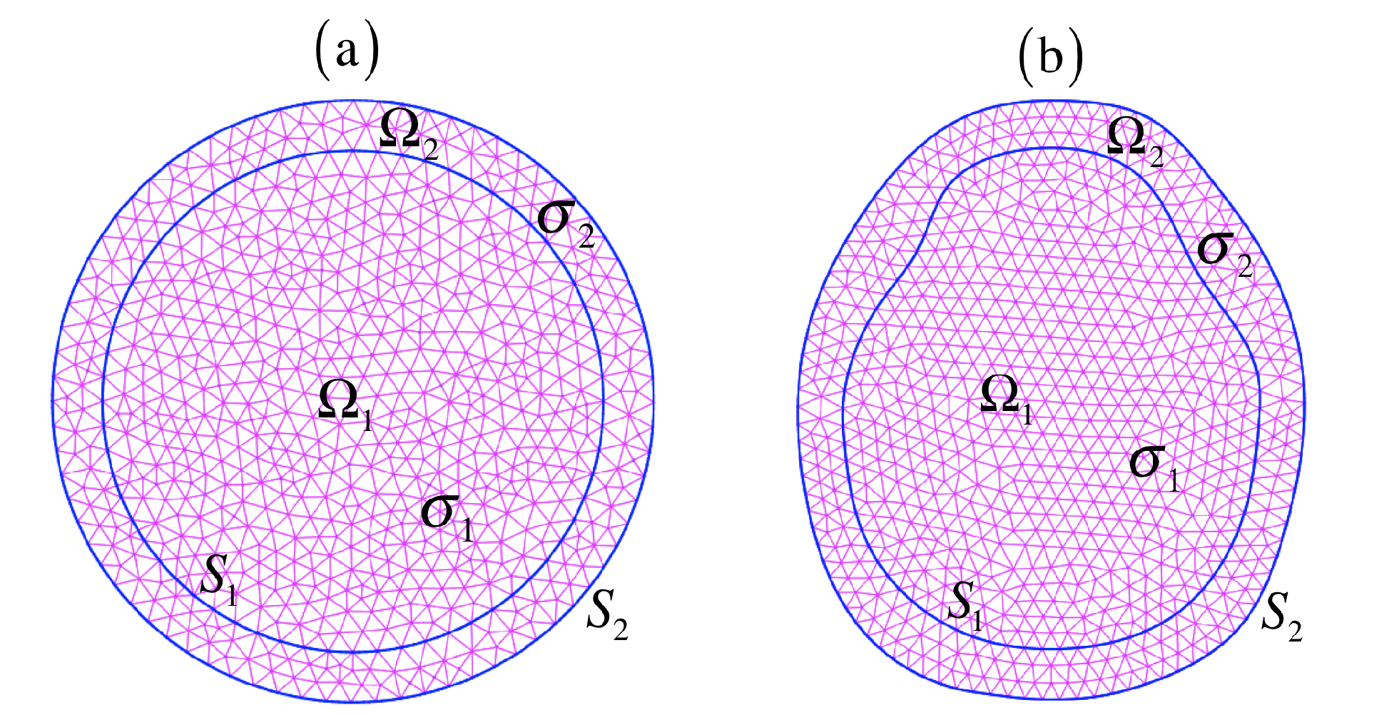
Based on two examples, we present the numerical results obtained using the methodology discussed in Section 6. Each example includes a different type of two-dimensional bounded region: a circular $\mathsf{\Omega }$ determined by two concentric circles centered in the origin, i.e., ${\mathsf{\Omega }}_1$ is a circular domain of radius $R_1$; ${\mathsf{\Omega }}_2$, which is a circular annular domain with interior radius $R_1$ and exterior radius $R_2$ (see Figure 1a), and the complex region shown in Figure 1b. The forward problem is solved by selecting a source g on $S_1$, followed by obtaining the solution u to the SBP (1)–(5) and then computing ${V=u|}_{S_2}$. Subsequently, the obtained potential V is provided as input data to the control problem (15) or cost function (14). Next, we consider examples with noiseless data V and noisy data $V_{\delta }$, where $\delta$ is the measurement error, i.e., ${∥V_{\delta }-V∥}_{L_2\left(S_2\right)}\le \delta$. The noisy data $V_{\delta }$ were obtained by adding a random error using the $rand$ function in MATLAB. Therefore, we define

$$\begin{array}{c}\hfill V_{\delta }=V+Error,\end{array}$$

(36)

where $Error=\delta max\left|V\right|\left[2rand\right(1,s)-1]$ is a vector of random numbers of length s, where s is the numbers of nodes on $S_2$.

Since the measurements are obtained by a device, they contain inherent error generated by different circumstances, such as rounding error (due to approximation or truncation), measurement handling, and device quality. We want to emphasize that the algorithm proposed works with different error levels. As an example, the electroencephalogram recorded on the scalp detects the voltage produced by bioelectrical activity and also detects artifacts produced by ocular and muscular movement. Thus, filters are applied to obtain a clean signal. Additionally, the sensitivity of the device generates errors.

However, we want to emphasize that the algorithm proposed works with different error levels. According to the numerical results, the error between the exact and approximate sources obtained by this method is proportional to the measurement error.

The corresponding approximate solution to problem (9) is denoted by $u_{1,h,k}^n$, and the corresponding approximate solution to state Equation (12) is denoted by $u_{2,h,k}^n$ and $V_{h,k}^n=u_{2,h,k}^n{|}_{S_2}$, where n denotes the number of conjugate gradient iterations to achieve a specific tolerance $\epsilon$, h is the size of the triangular mesh of $\mathsf{\Omega }$, and k is the penalization parameter. Moreover, their corresponding approximations to the normal derivative without and with sequential smoothing are denoted by ${\left.\frac{\partial u_{1,h,k}}{\partial n_1}\right|}_{S_1}$, ${\left.\frac{\partial u_{2,h,k}}{\partial n_1}\right|}_{S_1}$, ${\left.\frac{\partial u_{1,h,k,\overline{K}}}{\partial n_1}\right|}_{S_1}$, and ${\left.\frac{\partial u_{2,h,k,\overline{K}}}{\partial n_1}\right|}_{S_1}$, respectively, where $\overline{K}$ is the number of sequential smoothing. Finally, we denote $g_{h,k,\overline{K}}^n$ as the numerical approximation to g from the exact measurement V.

For noisy data $V_{\delta }$, the corresponding numerical solution is denoted by $u_{1,h,k\left(\delta \right)}$, $u_{2,h,k\left(\delta \right)}^n$, and $V_{h,k\left(\delta \right)}^n=u_{2,h,k\left(\delta \right)}^n{|}_{S_2}$.

In this case, the penalization parameter $k\left(\delta \right)=1/\alpha \left(\delta \right)$, where we assume

$$\alpha \left(\delta \right)=\delta =1/k\left(\delta \right),$$

(37)

thus, $\alpha \left(\delta \right)$ satisfies the Tikhonov criteria provided in Theorem 7.

The corresponding approximations to the normal derivative without and with the sequential smoothing of $u_{1,h,k\left(\delta \right)}$ and $u_{2,h,k\left(\delta \right)}^n$ are denoted by ${\left.\frac{\partial u_{1,h,k\left(\alpha \right)}}{\partial n_1}\right|}_{S_1}$, ${\left.\frac{\partial u_{2,h,k\left(\alpha \right)}}{\partial n_1}\right|}_{S_1}$, ${\left.\frac{\partial u_{1,h,k\left(\alpha \right),\overline{K}}}{\partial n_1}\right|}_{S_1}$, and ${\left.\frac{\partial u_{2,h,k\left(\alpha \right),\overline{K}}}{\partial n_1}\right|}_{S_1}$, respectively. Hence, we recovered an approximate stable source $g_{h,k\left(\delta \right),\overline{K}}^n$ from the measurement with error $V_{\delta }$.

For the numerical implementation of the proposed method in each example, we applied the finite element method to solve the elliptic problems that appeared in the algorithm proposed herein, using three different meshes. These meshes were denoted by $M_i(n{n}_i,n{e}_i)$, $i=1,2,3$, where $n{n}_i$ and $n{e}_i$ represent the number of nodes (vertices) and elements (triangles), respectively. Meshes $M_2$ and $M_3$ were obtained from successive regular refinements of the coarsest mesh $M_1$ with mesh size $h=0.1$. Figure 1a,b show the corresponding mesh $M_1$ of the circular and irregular region, respectively. Meshes $M_1$, $M_2$, and $M_3$ were generated using pdetool in MATLAB.

In the examples below, we considered the following absolute and relative errors for different values of $\delta$:

$$AE(g_{h,k\left(\delta \right),\overline{K}}^n,g)={\parallel g_{h,k\left(\delta \right),\overline{K}}^n-g\parallel }_{L_2\left(S_1\right)},$$

$$RE(g_{h,k\left(\delta \right),\overline{K}}^n,g)=\parallel g_{h,k\left(\delta \right),\overline{K}}^n{-g\parallel }_{L_2\left(S_1\right)}/{\parallel g\parallel }_{L_2\left(S_1\right)},$$

where $g_{h,k\left(\delta \right),\overline{K}}^n$ is the recovered source, and g is the exact source. Furthermore, we considered the relative error between the noisy data $V_{\delta }$ and noiseless data V, expressed as

$$RE(V_{\delta },V)=\parallel V_{\delta }{-V\parallel }_{L_2\left(S_2\right)}/{\parallel V\parallel }_{L_2\left(S_2\right)}.$$

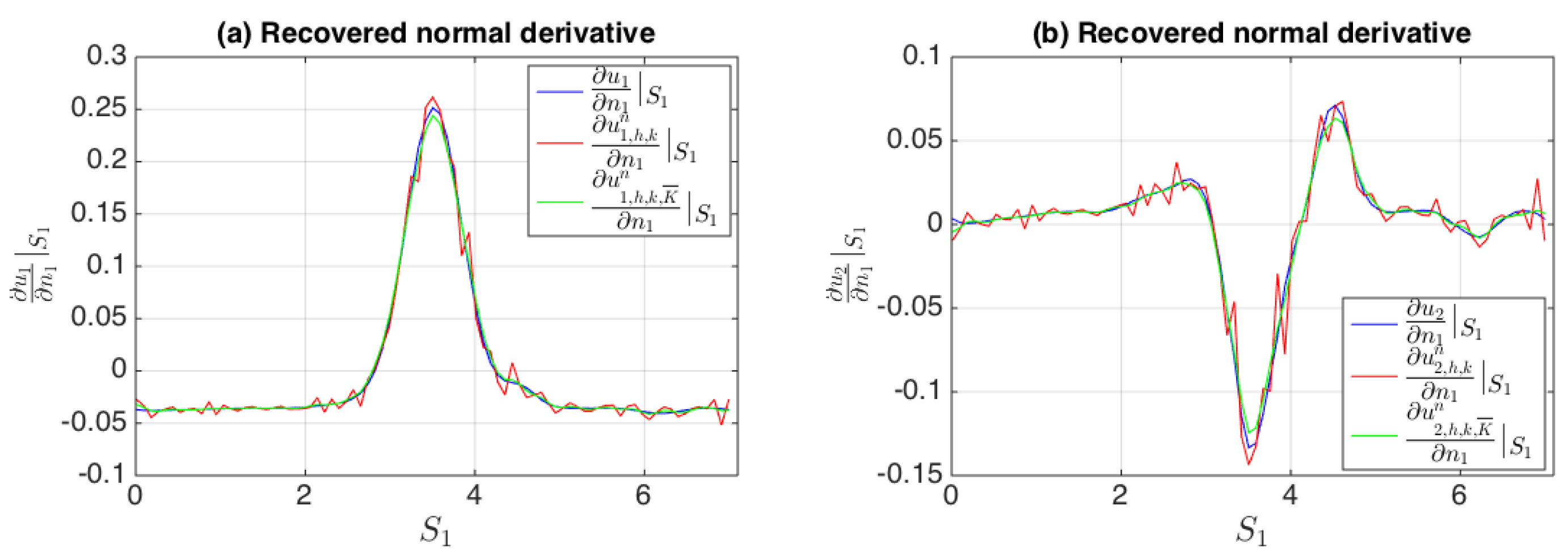
Example 1.

In this example, we considered the circular region Ω defined above, with ${\sigma }_1=3$, ${\sigma }_2=1$, $R_1=1$, and $R_2=1.2$. Let $g(x,y)=x^2-y^2$ for all $(x,y)\in S_1$ be the exact source; therefore, it belongs to $L_2\left(S_1\right)$ and satisfies condition (6). In polar coordinates, g is expressed as

$$g\left(\theta \right)=R_1^{2}cos\left(2\theta \right),for all \theta \in [0,2\pi ],$$

(38)

where the unique Fourier coefficient different from zero is $g_2^1=R_1^2$. Subsequently, the exact solution u to the SBP for the exact source g, using circular harmonics series, is

$$u_1(r,\theta )=\frac{\left(R_1^5+R_1{R}_2^4\right)r^{2}cos\left(2\theta \right)}{2\left[({\sigma }_1-{\sigma }_2)R_1^4+({\sigma }_1+{\sigma }_2)R_2^4\right]},$$

(39)

and

$$u_2(r,\theta )=\frac{\left(R_1^5{r}^2+R_1^5{R}_2^4{r}^{-2}\right)cos\left(2\theta \right)}{2\left[({\sigma }_1-{\sigma }_2)R_1^4+({\sigma }_1+{\sigma }_2)R_2^4\right]},$$

(40)

where their corresponding exact normal derivatives on the interior boundary $S_1$ are expressed as

$${\left.\frac{\partial u_1}{\partial n_1}\right|}_{S_1}=\frac{\left(R_1^6+R_1^2{R}_2^4\right)cos\left(2\theta \right)}{\left[({\sigma }_1-{\sigma }_2)R_1^4+({\sigma }_1+{\sigma }_2)R_2^4\right]},$$

(41)

$${\left.\frac{\partial u_2}{\partial n_1}\right|}_{S_1}=\frac{\left(R_1^6-R_1^2{R}_2^4\right)cos\left(2\theta \right)}{\left[({\sigma }_1-{\sigma }_2)R_1^4+({\sigma }_1+{\sigma }_2)R_2^4\right]}.$$

(42)

The solution to the forward problem for the exact source g is the exact measurement V provided in Equation (23), i.e.,

$$V\left(\theta \right)=\frac{R_1^5{R}_2^{2}cos\left(2\theta \right)}{\left[({\sigma }_1-{\sigma }_2)R_1^4+({\sigma }_1+{\sigma }_2)R_2^4\right]}.$$

(43)

Results for circular region with noiseless input data V. For the case of noiseless data V, the numerical results are summarized in

Table 1. Convergence of numerical results for circular region with noiseless data V, with $k={10}^{20}$ and $\epsilon ={10}^{-9}$.

Mesh	M${}_1(774,1470)$	M${}_2(3017,5880)$	M${}_3(\mathrm{11,913},\mathrm{23,520})$
n	26	11	10
$\overline{K}$	4	16	30
$Time$	$1.7715$ s	$4.1419$ s	$30.2689$ s
$AE(g_{h,k,\overline{K}}^n,g)$	$7.1486\times {10}^{-2}$	$5.0250\times {10}^{-2}$	$3.0647\times {10}^{-2}$
$RE(g_{h,k,\overline{K}}^n,g)$	$4.0355\times {10}^{-2}$	$2.8353\times {10}^{-2}$	$1.7291\times {10}^{-2}$

, where the following errors were included: $AE(g_{h,k,\overline{K}}^n,g)$, and $RE(g_{h,k,\overline{K}}^n,g)$. In this case, the penalization parameter, associated to the Cauchy problem, was set to $k={10}^{20}$, and we defined the stopping tolerance (which is the criterion used to stop the conjugate gradient method when the residual norm $\parallel g^{n+1}{\parallel }_{L_2\left(S_1\right)}^2\le \epsilon max\{1,\parallel g^0{\parallel }_{L_2\left(S_1\right)}^2\}$ for $n=0,1,2,\dots$ (see [29])) as $\epsilon ={10}^{-9}$. The relative errors decreased with each refinement of mesh $M_1$, showing the convergence of the discrete space. Moreover, the estimated computation times of the algorithm proposed for meshes $M_1$, $M_2$, and $M_3$ were $1.7715$, $4.1419$, and $30.2689$ s, respectively. The computation time of mesh $M_2$ was greater than that of mesh $M_1$ because the numbers of nodes (vertices) and elements (triangles) were greater than those in mesh $M_1$; furthermore, the number of smoothing increased. The computation time of mesh $M_3$ was the highest because the numbers of nodes (vertices), elements (triangles), and smoothing increased.

Figure 2 shows the exact source g and recovered source $g_{h,k,\overline{K}}^n$ (at iteration $n=26$) on $S_1$, for noiseless data V. The approximation is acceptable from the practical perspective. In fact, the highest relative error was $4.0355\times {10}^{-2}$, which was obtained using the coarsest mesh $M_1$, where $g_{h,k,\overline{K}}^n$ was calculated as shown in Step 3 of Section 6, i.e., by computing the approximate solutions $u_{1,h,k}^n$ and $u_{2,h,k}^n$ to problems (8) and (9) after applying the sequential smoothing method for computing their normal derivatives in stable form, as denoted by $\frac{\partial u_{1,k,h,\overline{K}}}{\partial n_1}$ and $\frac{\partial u_{2,k,h,\overline{K}}}{\partial n_1}$ on $S_1$, respectively. These are shown in Figure 3, where the number of sequential smoothing was $\overline{K}=4$. A similar behavior was observed when using meshes $M_2$ and $M_3$.

Results for circular region with noisy input data $V_{\delta }$. We selected the noisy data $V_{\delta }$ from Equation (36) and the coarsest mesh $M_1$. The values differed from the noiseless data $V,$ as $RE(V_{\delta },V)$ defined above.

Table 2. Convergence of numerical results for circular region with noisy data $V_{\delta }$ using mesh $M_1(774,1470)$ and $\epsilon ={10}^{-3}$.

Error $\mathit{\delta }$	0	0.001	0.01	0.1
$RE(V_{\delta },V)$	0	$8.5945\times {10}^{-4}$	$7.7607\times {10}^{-3}$	$7.7852\times {10}^{-2}$
$k\left(\delta \right)$	${10}^{20}$	${10}^3$	${10}^2$	10
n	1	1	1	1
$\overline{K}$	4	8	8	8
$Time$	$0.2117$ s	$0.2409$ s	$0.2418$ s	$0.2474$ s
$AE(g_{h,k\left(\delta \right),\overline{K}}^n,g)$	$8.8530\times {10}^{-2}$	$1.0381\times {10}^{-1}$	$1.0769\times {10}^{-1}$	$1.4784\times {10}^{-1}$
$RE(g_{h,k\left(\delta \right),\overline{K}}^n,g)$	$4.9977\times {10}^{-2}$	$5.8604\times {10}^{-2}$	$6.0794\times {10}^{-2}$	$8.3461\times {10}^{-2}$

shows the results for the circular region for different values of δ, from where we observed that the numerical solutions $g_{h,k\left(\delta \right),\overline{K}}^n$ converged to the noiseless solutions $g_{h,k,\overline{K}}^n$ as δ approached zero; this demonstrates the stability of the numerical results against perturbations in measurement V for the circular region. In addition, the computation time of the algorithm proposed for each value of δ was $0.2117$, $0.2409$, $0.2418$, and $1.2474$ s, with $\overline{K}=8$. The computation time for $\delta =0$ was the lowest because the number of smoothing was minor ($\overline{K}=4$).

Figure 4 shows the plots of the exact measurement V, recovered data $V_{h,k\left(\delta \right)}^n$ with measurement with error $V_{\delta }$ when $\delta =0.1$, and corresponding recovered source $g_{h,k\left(\delta \right),\overline{K}}^n$ (at iteration $n=1$) on $S_1$ that was calculated as shown in Step 3 of Section 6. Figure 5 shows the smoothing normal derivatives $\frac{\partial }{\partial n_1}\left(u_{1,h,k\left(\delta \right),\overline{K}}^n\right)$ and $\frac{\partial }{\partial n_1}\left(u_{2,h,k\left(\delta \right),\overline{K}}^n\right)$ from the corresponding recovered derivatives of $u_{1,h,k\left(\delta \right)}^n$ and $u_{2,h,k\left(\delta \right)}^n$, respectively. In this case, the penalization parameter $k\left(\delta \right)$ was selected as in the case of noisy data $V_{\delta }$, i.e., $k\left(\delta \right)={\delta }^{-1}$. The stopping tolerance was $\epsilon ={10}^{-3}$, and the number of smoothing was $\overline{K}=8$ for $\delta =0.001$, $0.01$, and $0.1$. In this case, the highest relative error between the exact source g and the recovered source $g_{h,k\left(\delta \right),\overline{K}}^n$ was $8.3461\times {10}^{-2}$ using the coarsest mesh $M_1$. We observed that the recovered solutions $g_{h,k\left(\delta \right),\overline{K}}^n$ converged to the exact solution g when δ approached zero.

Example 2.

For this case, we considered the complex region shown in Figure 1b and the exact source g expressed as

$$\begin{array}{c}\hfill g(x,y)=f(x,y)-\frac{1}{m\left(S_1\right)}{\int }_{S_1}f(x,y)ds,\end{array}$$

(44)

for all $(x,y)\in S_1$ where $f(x,y)=e^{-\frac{\parallel (x,y)-(a_1,a_2){\parallel }^2}{2{\beta }^2}}$, m denotes the Lebesgue measure on $\mathbb{R}$, ${\beta }^2=0.1$, and $(a_1,a_2)=(-1.0067,0.0093)\in S_1$. In this case, g belongs to $L_2\left(S_1\right)$ and satisfies condition (6).

Furthermore, the exact solution u to the SBP and the exact measurement ${V=u|}_{S_2}$ (for this source g) were calculated numerically using the finite element method and a very fine mesh, which we denote as $M_4$. This mesh was obtained after three regular refinements of the starting mesh, i.e., $M_1$ shown in Figure 1b. In addition, we computed the exact normal derivatives of $u_1$ and $u_2$ on the interior boundary $S_1$, as shown in Equations (25) and (26), respectively, using the exact solution u calculated based on the finest mesh $M_4$.

Results for irregular region with noiseless data V. The numerical results in

Table 3. Convergence of numerical results for irregular region with noiseless data V, where $k={10}^{20}$ and $\epsilon ={10}^{-9}$.

Mesh	M${}_1(855,1607)$	M${}_2(3316,6428)$	M${}_3(\mathrm{13,059},\mathrm{25,712})$
n	24	24	24
$\overline{K}$	4	16	30
$Time$	$1.6713$ s	$7.5117$ s	$84.2667$ s
$AE(g_{h,k,\overline{K}}^n,g)$	$3.3334\times {10}^{-2}$	$3.2655\times {10}^{-2}$	$3.2107\times {10}^{-2}$
$RE(g_{h,k,\overline{K}}^n,g)$	$4.8550\times {10}^{-2}$	$4.7556\times {10}^{-2}$	$4.6756\times {10}^{-2}$

show the convergence regarding the discrete space of the complex domain Ω for the source g defined in Equation (44), with the penalization parameter $k={10}^{20}$ and stopping tolerance $\epsilon ={10}^{-9}$.

The computation time in mesh $M_3$ was the highest because mesh $M_3$ was the finest, i.e., the numbers of nodes (vertices) and elements (triangles) were greater than those in meshes $M_1$ and $M_2$, and the number of smoothing increased to 30 in mesh $M_3$. We observed that the relative numerical errors on the interior boundary, $RE(g_{h,k,\overline{K}}^n,g)$, were slightly higher for the complex region because the interior boundary $S_1$ was more complex than the corresponding circular region. In addition, the number of conjugate gradient iterations for achieving the desired accuracy was higher for the complex region presented in meshes $M_2$ and $M_3$.

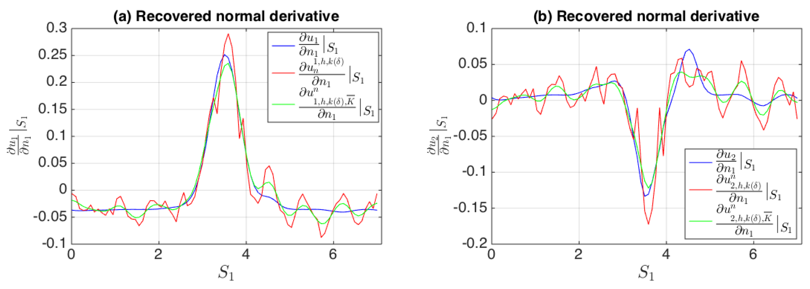
Figure 6 shows the exact g and recovered sources $g_{h,k,\overline{K}}^n$ (at iteration $n=24$) on $S_1$, for noiseless data V. In this case, the highest relative error of $4.8550\times {10}^{-2}$ was observed in the coarsest mesh $M_1$. A similar behavior was observed when using meshes $M_2$ and $M_3$. The plots of the exact normal derivatives of $u_1$ and $u_2$ and their corresponding approximations without and with sequential smoothing corresponding to the input data without error V are shown in Figure 7, where the number of sequential smoothing was $\overline{K}=4$.

Results for irregular region with noisy input data $V_{\delta }$.

Table 4. Convergence of numerical results for irregular region with noisy data $V_{\delta }$ using mesh $M_1(855,1607)$ and $\epsilon ={10}^{-3}$.

Error $\mathit{\delta }$	0	0.001	0.01	0.1
$RE(V_{\delta },V)$	0	$1.3855\times {10}^{-3}$	$1.5028\times {10}^{-2}$	$1.2549\times {10}^{-1}$
$k\left(\delta \right)$	${10}^{20}$	${10}^3$	${10}^2$	10
n	2	2	2	2
$\overline{K}$	4	10	10	10
$Time$	$0.3082$ s	$0.3253$ s	$0.3297$ s	$0.3338$ s
$AE(g_{h,k\left(\delta \right),\overline{K}}^n,g)$	$1.1357\times {10}^{-1}$	$1.1416\times {10}^{-1}$	$1.1536\times {10}^{-1}$	$1.1680\times {10}^{-1}$
$RE(g_{h,k\left(\delta \right),\overline{K}}^n,g)$	$1.6541\times {10}^{-1}$	$1.6628\times {10}^{-1}$	$1.6802\times {10}^{-1}$	$1.7011\times {10}^{-1}$

shows the numerical results for the complex region when the input data V were perturbed, as in Equation (36) for source in Equation (44), using mesh $M_1$ of the complex region Ω shown in Figure 1b. In each case, one can observe that the qualitative behavior was similar to that of the circular region, and the highest relative error of the approximate solution $g_{h,k\left(\delta \right),\overline{K}}^n$ was $1.7011\times {10}^{-1}$ in the coarsest mesh $M_1$. In addition, in this mesh, the computation time for $\delta =0$ was lower than for $\delta =0.001$, $0.01$, and $0.1$ because the number of smoothing was lesser ($\overline{K}=4$). The numerical solutions $g_{h,k\left(\delta \right),\overline{K}}^n$ converged to $g_{h,k,\overline{K}}^n$ when δ approached zero, demonstrating the stability of the numerical results against perturbations in the irregular region.

Figure 8 shows the plots of the exact measurement V, recovered data $V_{h,k\left(\delta \right)}^n$ with measurement error $V_{\delta }$ when $\delta =0.1$ (left), and corresponding recovered source $g_{h,k\left(\delta \right),\overline{K}}^n$ (at iteration $n=2$) on $S_1$ of the irregular region (right), which was calculated using the algorithm proposed in Section 6. Figure 9 shows the normal derivatives without and with the sequential smoothing of $u_{1,h,k\left(\delta \right)}^n$ and $u_{2,h,k\left(\delta \right)}^n$. In this case, the penalization parameter $k\left(\delta \right)$ was selected, as in the case of noisy data $V_{\delta }$, i.e., $k\left(\delta \right)={\delta }^{-1}$. The stopping tolerance was $\epsilon ={10}^{-3}$, and the number of smoothing was $\overline{K}=10$. In this case, the highest relative error between the exact source g and recovered source $g_{h,k\left(\delta \right),\overline{K}}^n$ was $1.7011\times {10}^{-1}$ in the coarsest mesh $M_1$.

Therefore, we demonstrated that our approach yielded convergent solutions that were stable against perturbations of the input data V in circular and irregular nonhomogeneous region media Ω.

Comparison with Other Method

We present the comparison of the solutions to the inverse source problem using the method proposed in this work that we called Method 1 (see Section 6) and the one presented in reference [30] that we called Method 2, which uses operator A shown in Section 2.3 (Operational statement).

We consider the circular and irregular region given in the examples from this section with the same values for $R_1=1$, $R_2=1.2$, ${\sigma }_1=3$, and ${\sigma }_2=1$. In the case of the circular region $\mathsf{\Omega }$, we consider the exact source $g(x,y)=x^2-y^2$, for all $(x,y)\in S_1$, that in polar coordinates is given by (38), and the exact source g given by (44) with ${\beta }^2=0.1$ and $(a_1,a_2)=(-1,0)\in S_1$, that expressed in polar coordinates takes the form

$$g\left(\theta \right)=f_1(R_1,\theta )-\frac{1}{2\pi }{\int }_0^{2\pi }{f}_1(R_1,\theta )d\theta ,for all \theta \in [0,2\pi ],$$

(45)

where $f_1(R_1,\theta )=e^{\frac{-R_1^2+R_1^{2}cos(\theta -{\theta }_0)}{2{\beta }^2}}$, for all $\theta \in [0,2\pi ]$, ${\theta }_0=\pi$, and ${\beta }^2=0.1$.

In this case, g belongs to $L_2\left(S_1\right)$ and satisfies condition (6). For this exact source g, we approximated function $g\in L_2\left(S_1\right)$ by its truncated Fourier series $g_{{}_N}$ using the first N terms. In this case, both the exact solution u to the forward problem (1)–(5) and the exact measurement are generated with the first $N=30$ terms of the Fourier series (21)–(23), and $\parallel g-g_N{\parallel }_{L_2\left(S_1\right)}=1.4011\times {10}^{-8}$. The Fourier coefficients $g_k^1$, $g_k^2$, $k=1,2,\dots ,N$ are obtained numerically using the function quadl of MATLAB. The plots of g and its approximation $g_N$ are shown in Figure 10. In the following, we denote the approximation $g_N$ by g.

In the case of the irregular region $\mathsf{\Omega }$ shown in Figure 1b, we considered the exact source g given by (44), with the same values for ${\beta }^2=0.1$ and $(a_1,a_2)=(-1.0067,0.0093)\in S_1$, and the exact source g expressed as

$$\begin{array}{c}\hfill g(x,y)=f_2(x,y)-\frac{1}{m\left(S_1\right)}{\int }_{S_1}{f}_2(x,y)ds,\end{array}$$

(46)

for all $(x,y)\in S_1$, where $f_2(x,y)=x^2-y^2$. In this case, g belongs to $L_2\left(S_1\right)$ and satisfies condition (6) too. Furthermore, the exact solution u to the forward problem (1)–(5) and the exact measurement ${V=u|}_{S_2}$ (for this source g) were calculated numerically using the finite element method with the finest mesh $M_4$ of the irregular region $\mathsf{\Omega }$. In addition, we computed the exact normal derivatives of $u_1$ and $u_2$ on the interior boundary $S_1$, as shown in Equations (25) and (26), respectively, using the exact solution u calculated based on the finest mesh $M_4$.

Table 5. Numerical results applying methods 1 and 2 for circular region with noisy data $V_{\delta }$ for $\delta =0.1$, using mesh $M_1(774,1470)$, and with the same measurement with error $V_{\delta }$ for each source. NA means not applicable.

Method	Method 1		Method 2
Parameters	$\mathit{k}\left(\mathit{\delta }\right)=\mathbf{10}$, $\overline{\mathit{K}}=\mathbf{8}$, $\mathit{\epsilon }={\mathbf{10}}^{-\mathbf{3}}$.		$\mathit{\alpha }\left(\mathit{\delta }\right)={\mathbf{10}}^{-\mathbf{4}}$, $\mathit{\epsilon }={\mathbf{10}}^{-\mathbf{3}}$
Source	$\mathit{g}$ Given by (38)	$\mathit{g}$ Given by (45)	$\mathit{g}$ Given by (38)	$\mathit{g}$ Given by (45)
$RE(V_{\delta },V)$	$7.8801\times {10}^{-2}$	$1.3435\times {10}^{-1}$	$7.8801\times {10}^{-2}$	$1.3435\times {10}^{-1}$
n	1	2	3	6
$Time$	$0.2481$ s	$0.2878$ s	$0.5085$ s	$1.0083$ s
$RE(g_{h,k\left(\delta \right),\overline{K}}^n,g)$	$6.8223\times {10}^{-2}$	$1.8430\times {10}^{-1}$	NA	NA
$RE(g_{h,\alpha \left(\delta \right)}^n,g)$	NA	NA	$2.3730\times {10}^{-2}$	$2.8285\times {10}^{-1}$

and

Table 6. Numerical results applying methods 1 and 2 for irregular region with noisy data $V_{\delta }$ for $\delta =0.1$, using mesh $M_1(855,1607)$, and with the same measurement with error $V_{\delta }$ for each source. NA means not applicable.

Method	Method 1		Method 2
Parameters	$\mathit{k}\left(\mathit{\delta }\right)=\mathbf{10}$, $\overline{\mathit{K}}=\mathbf{10}$, $\mathit{\epsilon }={\mathbf{10}}^{-\mathbf{3}}$		$\mathit{\alpha }\left(\mathit{\delta }\right)={\mathbf{10}}^{-\mathbf{4}}$, $\mathit{\epsilon }={\mathbf{10}}^{-\mathbf{3}}$
Source	$\mathit{g}$ Given by (46)	$\mathit{g}$ Given by (44)	$\mathit{g}$ Given by (46)	$\mathit{g}$ Given by (44)
$RE(V_{\delta },V)$	$1.0632\times {10}^{-1}$	$1.4033\times {10}^{-1}$	$1.0632\times {10}^{-1}$	$1.4033\times {10}^{-1}$
n	2	2	5	7
$Time$	$0.3017$ s	$0.3308$ s	$0.8931$ s	$1.2059$ s
$RE(g_{h,k\left(\delta \right),\overline{K}}^n,g)$	$1.3018\times {10}^{-1}$	$1.7255\times {10}^{-1}$	NA	NA
$RE(g_{h,\alpha \left(\delta \right)}^n,g)$	NA	NA	$9.6094\times {10}^{-2}$	$2.9382\times {10}^{-1}$

show the numerical results for the circular and irregular region for input noisy data $V_{\delta }$, for $\delta =0.1$ in mesh $M_1$ of each region, respectively, and where the computation time and the following relative errors are included: $RE(g_{h,k\left(\delta \right),\overline{K}}^n,g)$, $RE(g_{h,\alpha \left(\delta \right)}^n,g)$ of each method, where $g_{h,\alpha \left(\delta \right)}^n$ is the corresponding recovered source given by Method 2. In this case, the regularization parameter $\alpha \left(\delta \right)$ was chosen by the L-curve method.

In order to compare the efficiency of Methods 1 and 2, we considered the same measurement with error $V_{\delta }$ of each source g in each region $\mathsf{\Omega }$, and the same stopping tolerance $\epsilon ={10}^{-3}$ for the conjugate gradient method proposed in Methods 1 and 2. In this case, the regularization parameter $\alpha \left(\delta \right)={10}^{-3}$ for the circular region and $\alpha \left(\delta \right)={10}^{-4}$ for the irregular region. From the numerical results, we observed the following important properties (for $\delta =0.1$): (a) All relative errors corresponding to the sources recovered by each method are proportional to the relative perturbation $E{R}_{S_2}(V_{\delta },V)$, showing the stability of the numerical results regarding perturbations for the circular and irregular region, respectively; (b) All relative errors corresponding to the sources recovered by each method are of the same order in each region $\mathsf{\Omega }$; (c) The computation time of Method 1 was lower than that of Method 2, because Method 1 solves the Cauchy problem for the Laplace Equation (using the conjugate gradient method provided in [29]), in the smaller sub-region ${\mathsf{\Omega }}_2$ contained in $\mathsf{\Omega }$ and with a smaller number of iterations than Method 2 that solves the inverse problem applying the conjugate gradient method proposed in [30], wherein each iteration two elliptical problems are solved in the largest region $\mathsf{\Omega }$. In addition, Method 1 also includes the computation time to solve the Dirichlet problem for the Laplace equation in the smaller sub-region ${\mathsf{\Omega }}_1$ contained in $\mathsf{\Omega }$ (which is calculated only once), the calculation of normal derivatives and the applying of the sequential smoothing method for the calculation of the stable derivatives, and the calculation of the recovered source $g_{h,k\left(\delta \right),\overline{K}}^n$ using formula (10).

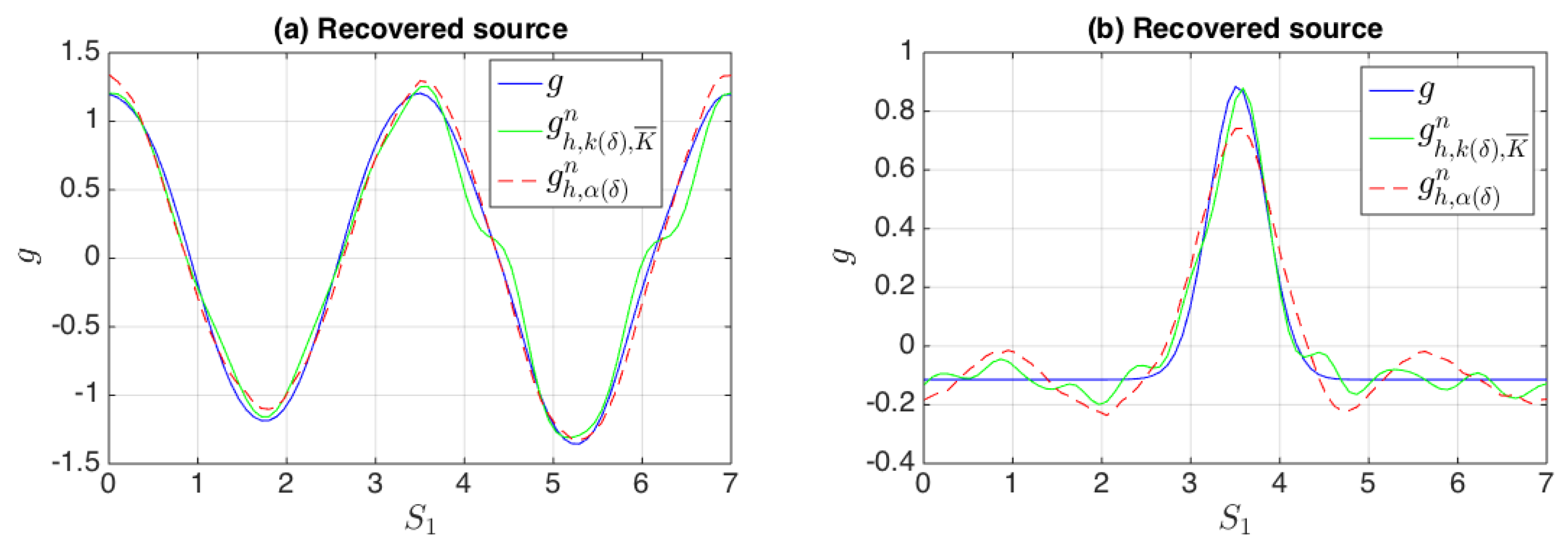
The plots of the sources recovered from the measurement with error $V_{\delta }$ ($\delta =0.1$) by each method are shown in Figure 11 and Figure 12, using mesh $M_1$ of the circular and irregular region, respectively.

From Table 5 and Table 6, we observed that the method proposed in this work is better, regarding the computational cost, than the one presented in [30]. Furthermore, the relative errors of the sources recovered by Method 1 are of the same order as the ones recovered by Method 2, which are proportional to the relative perturbation $RE(V_{\delta },V)$, showing the stability of the numerical results regarding perturbations for both the circular and irregular region.

8. Discussion

In this work, we presented a stable algorithm for recovering sources located on the interface that separates two homogeneous media (which compound the nonhomogeneous media studied in this work). This algorithm works for simple and complex geometries and consists of three steps given in Section 6. Each problem is solved appropriately. Two of them present numerical instability, namely, the Cauchy problem for the Laplace equation defined in an annular region and the calculation of the normal derivatives, which involves the derivative operator that is discontinuous. We consider the results given in [29], in which an operational statement of the problem with a linear, injective and compact operator defined between Hilbert spaces is used. The ill-posedness due to the numerical instability of the Cauchy problem is proved using this operational statement. A control approach and the Tikhonov regularization are considered to handle the numerical instability. We used the sequential smoothing method as a regularization technique for the stable calculations of the derivatives. In some inverse problems, such as inverse electroencephalography and capacitance tomography it is necessary to obtain the normal derivatives to find the solution to these inverse problems [20,36]. This work shows the feasibility of applying the sequential smoothing method to find the normal derivatives in a stable form. The sequential smoothing method is simple to program and apply. In [30], the authors presented another method to find the source in which it is not necessary to find the normal derivatives that represent a disadvantage regarding the method presented in this work. Furthermore, the computational cost is lower in the method presented here. In this work, we numerically chose the number of sequential smoothing. One interesting point is to find a theoretical result to choose the number of sequential smoothing in terms of the measurement error (taking into account the results for the Cauchy problem). We consider this point in future work. Finally, we want to emphasize that the algorithm presented in this work can be extended to a region $\mathsf{\Omega }$ in the 3D space.

9. Conclusions

The problem of identifying sources defined on separation interfaces in nonhomogeneous media can be solved in a stable form using the proposed algorithm, which can be applied to regions with simple and complex geometries. Its efficiency was demonstrated based on two examples involving nonhomogeneous circular and irregular regions. The numerical results demonstrated the convergence and stability of the algorithm regarding the input data with and without noise. The algorithm employs the penalization and sequential smoothing methods, where the penalization parameter can be selected as the inverse of the Tikhonov regularization parameter, whereas the number of sequential smoothing $\overline{K}$ can be selected based on the residual principle. The sequential smoothing method allows us to find the normal derivatives of the potentials on the separation interface in a stable form.

References

1. Friston, K.; Harrison, L.; Daunizeau, J.; Kiebel, S.; Phillips, C.; Trujillo, N.; Henson, R.; Flandin, G.; Mattout, J. Multiple sparse priors for the M/EEG inverse problem. NeuroImage 2008, 39, 1104–1120. [Google Scholar] [CrossRef]
2. Hamad, A.; Tadi, M. A numerical method for inverse source problems for Poisson and Helmholtz equations. Annalen der Physik 2016, 380, 3707–3716. [Google Scholar] [CrossRef]
3. Hämäläinen, M.; Hari, R.; Ilmoniemi, R.J.; Knuutila, J.; Lounasmaa, O.V. Magnetoencephalography—Theory, instrumentation, and applications to noninvasive studies of the working human brain. Rev. Mod. Phys. 1993, 65, 413–497. [Google Scholar] [CrossRef] [Green Version]
4. Ioannides, A.; Bolton, J.P.R.; Clarke, C.J.S. Continuous probabilistic solutions to the biomagnetic inverse problem. Inverse Probl. 1990, 6, 523–542. [Google Scholar] [CrossRef]
5. Jin, B.; Marin, L. The method of fundamental solutions for inverse source problems associated with the steady-state heat conduction. Int. J. Numer. Meth. Eng. 2007, 69, 1570–1589. [Google Scholar] [CrossRef]
6. Nguyen, P.M.; Nguyen, L.H. A numerical method for an inverse source problem for parabolic equations and its application to a coefficient inverse problem. J. Inverse Ill-Posed Probl. 2020, 28, 323–339. [Google Scholar] [CrossRef] [Green Version]
7. Widman, L.E. Computational inverse problems in electrocardiography. J. Biomed. Inform. 2002, 35, 51. [Google Scholar] [CrossRef] [Green Version]
8. Yan, L.; Yang, F.L.; Fu, C.L. A new numerical method for the inverse source problem from a Bayesian perspective. Int. J. Numer. Meth. Eng. 2011, 85, 1460–1474. [Google Scholar] [CrossRef]
9. Zidarov, D. Inverse Gravimetric Problem in Geoprospecting and Geodesy, 2nd ed.; Elsevier: Amsterdam, The Netherlands, 1990. [Google Scholar]
10. Saad, F.O.; Sdayria, A.; Madiouli, J.; Sghaier, J.; Fudym, O. Quadrupole method: A new approach for solving the direct problem of electrical resistance tomography. J. King Saud Univ. Sci. 2017, 29, 360–370. [Google Scholar] [CrossRef]
11. Huntul, M.J.; Lesnic, D. Reconstruction of the timewise conductivity using a linear combination of heat flux measurements. J. King Saud Univ. Sci. 2020, 32, 928–933. [Google Scholar] [CrossRef]
12. Abdelaziz, B.; EL Badia, A.; Hajj, A.E. Direct algorithms for solving some inverse source problems in 2D elliptic equations. Inverse Probl. 2015, 31, 1–26. [Google Scholar] [CrossRef] [Green Version]
13. El Badia, A.; Ha Duong, T.; Moutazaim, F. Numerical solution for the identification of source terms from boundary measurements. Inverse Probl. Eng. 2000, 8, 345–364. [Google Scholar] [CrossRef]
14. El Badia, A.; Farah, M. Identification of dipole sources in an elliptic equation from boundary measurements: Application to the inverse EEG problem. J. Inverse Ill-Posed Probl. 2006, 14, 331–353. [Google Scholar] [CrossRef]
15. Fraguela, A.; Oliveros, J.; Grebennikov, A. Operational statement and analysis of the inverse electroencephalographic problem. Rev. Mex. Fis. 2001, 47, 162–174. (In Spanish) [Google Scholar]
16. Caulier-Cisterna, R.; Muñoz-Romero, S.; Sanroman-Junquera, M.; Garcia- Alberola, A.; Rojo-Álvarez, J.L. A new approach to the intracardiac inverse problem using Laplacian distance kernel. Biomed. Eng. Online 2018, 17, 1–25. [Google Scholar] [CrossRef] [PubMed] [Green Version]
17. Fraguela, A.; Oliveros, J.; Morín, M.; Cervantes, L. Inverse electroencephalography for cortical sources. Appl. Numer. Math. 2005, 55, 191–203. [Google Scholar] [CrossRef]
18. Kalinin, A.; Potyagaylo, D.; Kalinin, V. Solving the inverse problem of electrocardiography on the endocardium using a single layer source. Front. Physiol. 2019, 10, 1–13. [Google Scholar] [CrossRef] [Green Version]
19. Morín-Castillo, M.; Netzahualcoyotl-Bautista, C.; Conde-Mones, J.; Oliveros-Oliveros, J.; Santillán-Guzmán, A. Stable identification of sources associated with epileptic focus on the cerebral cortex. Rev. Mex. Ing. Biomed. 2019, 40, 1–14. [Google Scholar]
20. Oliveros-Oliveros, J.; Morín-Castillo, M.; Aquino-Camacho, F.; Fraguela-Collar, A. Analysis of the inverse electroencephalographic problem for volumetric dipolar sources using a simplification. Rev. Mex. Ing. Biomed. 2014, 35, 115–124. [Google Scholar]
21. Revishvili, A.S.; Wissner, E.; Lebedev, D.S.; Lemes, C.; Deiss, S.; Metzner, A.; Kalinin, V.V.; Sopov, O.V.; Labartkava, E.Z.; Kalinin, A.V.; et al. Validation of the mapping accuracy of a novel non-invasive epicardial and endocardial electrophysiology system. Europace 2015, 17, 1282–1288. [Google Scholar] [CrossRef] [Green Version]
22. Richter, M. Inverse Problems: Basics, Theory and Applications in Geophysics; Birkhäuser: Basel, Switzerland, 2016. [Google Scholar]
23. Zhdanov, M.S. Inverse Theory and Applications in Geophysics; Elsevier: Amsterdam, The Netherlands, 2015. [Google Scholar]
24. Azis, M.I.; Solekhudin, I.; Aswad, M.H.; Jalil, A.R. Numerical simulation of two-dimensional modified Helmholtz problems for anisotropic functionally graded materials. J. King Saud Univ. Sci. 2020, 32, 2096–2102. [Google Scholar] [CrossRef]
25. Balali, Z.; Rashidinia, J.; Taheri, N. Numerical solution of singular boundary value problems using Green’s function and Sinc-Collocation method. Annalen der Physik 2020, 32, 2962–2968. [Google Scholar]
26. Karageorghis, A.; Lesnic, D.; Marin, L. A survey of applications of the MFS to inverse problems. Inverse Probl. Sci. Eng. 2011, 19, 309–336. [Google Scholar] [CrossRef]
27. Reza-E-Rabbi, S.; Arifuzzaman, S.M.; Sarkar, T.; Khan, M.S.; Ahmmed, S.F. Explicit finite difference analysis of an unsteady MHD flow of a chemically reacting casson fluid past a stretching sheet with brownian motion and thermophoresis effects. J. King Saud Univ. Sci. 2020, 32, 690–701. [Google Scholar] [CrossRef]
28. Glowinski, R. Finite Element Methods for Incompressible Viscous Flow; Elsevier: Amsterdam, The Netherlands, 2003. [Google Scholar]
29. Conde, J.J.; Juárez, L.H.; Oliveros, J.J.; León, D.A. Stable numerical solution of the Cauchy problem for the Laplace equation in irregular annular regions. Numer. Methods Partial Differ. Equ. 2017, 33, 1799–1822. [Google Scholar] [CrossRef]
30. Morín-Castillo, M.M.; Netzahualcoyotl-Bautista, C.; Oliveros-Oliveros, J.J.; Conde-Mones, J.J.; Juárez-Valencia, L.H. Stable identification of sources located on separation interfaces of two different homogeneous media. Adv. Differ. Equ. Control Process. 2019, 20, 53–97. [Google Scholar] [CrossRef]
31. Pérez-Becerra, T.; Sánchez-Perales, S.; Oliveros-Oliveros, J.J. The HK-Sobolev space and applications to one-dimensional boundary value problems. J. King Saud Univ. Sci. 2020, 32, 2790–2796. [Google Scholar] [CrossRef]
32. León-Velasco, D.; Morín-Castillo, M.; Oliveros-Oliveros, J.; Pérez-Becerra, T.; Escamilla-Reyna, J. Numerical solution of some differential equations with Henstock–Kurzweil functions. J. Funct. Space. 2019, 2019, 1–9. [Google Scholar] [CrossRef]
33. Kirsch, A. An Introduction to the Mathematical Theory of Inverse Problems, 2nd ed.; Springer Science & Business Media: Berlin, Germany, 2011. [Google Scholar]
34. Yang, F.; Fu, C.-L. A simplified Tikhonov regularization method for determining the heat source. Appl. Math. Model. 2010, 34, 3286–3299. [Google Scholar] [CrossRef]
35. Brenner, S.C.; Scott, L.R. The Mathematical Theory of Finite Element Methods, 3rd ed.; Springer: New York, NY, USA, 2008. [Google Scholar]
36. Fraguela, A.; Oliveros, J.; Cervantes, L.; Morín, M.; Gómez, S. A non-iterative algorithm for the electrical capacitance tomography (in Spanish). Rev. Mex. Fis. 2005, 51, 236–242. [Google Scholar]
37. Hao, D.N.; Lesnic, D. The Cauchy problem for Laplace’s equation via the conjugate gradient method. IMA J. Appl. Math. 2000, 65, 199–217. [Google Scholar] [CrossRef]
38. Glowinski, R.; Lions, J.L.; He, J.W. Exact and Approximate Controllability for Distributed Parameter Systems: A Numerical Approach; Cambridge University Press: Cambridge, MA, USA, 2008. [Google Scholar]
39. Hansen, P.C. The L-curve and its use in the numerical treatment of inverse problems. In Computational Inverse Problems in Electrocardiology; Johnston, P., Ed.; WIT Press: Southampton, UK, 2001; pp. 119–142. [Google Scholar]
40. Morozov, V.A.; Grebennikov, A.I. Methods for Solution of Ill-Posed Problems: Algorithmic Aspects, 3rd ed.; University Press: Moscow, Russia, 2005. [Google Scholar]
41. Grebennikov, A. Splines Methods: Theoretical Elements, Algorithms and Programs, 3rd ed.; Max Press: Moscow, Russia, 2008. (In Spanish) [Google Scholar]
Figure 1. Two representations of region Ω = Ω ¯ 1 Ω 2 . Source g is defined on interface S 1 . (a) Circular region Ω , (b) Irregular region Ω .
Mathematics 09 01932 g001
Figure 2. (a) Plots of exact data V (black) and recovered data V h , k n (blue). (b) Plots of exact source g (blue) and recovered source g h , k , K ¯ n (green) on S 1 , corresponding to exact input data V, using mesh M 1 of circular region Ω.
Mathematics 09 01932 g002
Figure 3. (a) Plots of exact normal derivative of u 1 and its approximations with and without sequential smoothing corresponding to input data without error V, using mesh M 1 of circular region. (b) Plots of exact normal derivative of u 2 and its approximations with and without sequential smoothing corresponding to input data without error V, using mesh M 1 of circular region.
Mathematics 09 01932 g003
Figure 4. (a) Plots of exact data V (black), data with error V δ (red), and recovered data V h , k ( δ ) n (blue), for δ = 0.1 . (b) Plots of exact source g (blue) and recovered source g h , k ( δ ) , K ¯ n (green) on S 1 , corresponding to data with noise V δ , using mesh M 1 of circular region Ω.
Mathematics 09 01932 g004
Figure 5. (a) Plots of exact normal derivative of u 1 and its approximations with and without sequential smoothing corresponding to input data with error V δ , using mesh M 1 of circular region. (b) Plots of exact normal derivative of u 2 and its approximations with and without sequential smoothing corresponding to input data with error V δ , using mesh M 1 of circular region.
Mathematics 09 01932 g005
Figure 6. (a) Plots of exact data V (black) and recovered data V h , k n (blue). (b) Exact source g (blue) and recovered source g h , k , K ¯ n (green) on S 1 , corresponding to exact input data V, using mesh M 1 of irregular region Ω.
Mathematics 09 01932 g006
Figure 7. (a) Plots of exact normal derivative of u 1 and its approximations with and without sequential smoothing corresponding to input data without error V, using mesh M 1 of irregular region. (b) Plots of exact normal derivative of u 2 and its approximations with and without sequential smoothing corresponding to input data without error V, using mesh M 1 of irregular region.
Mathematics 09 01932 g007
Figure 8. (a) Plots of exact data V (black), data with error V δ (red), and recovered data V h , k ( δ ) n (blue), for δ = 0.1 . (b) Plots of exact source g (blue) and recovered source g h , k ( δ ) , K ¯ n (green) on S 1 , corresponding to data with noise V δ using mesh M 1 of irregular region Ω.
Mathematics 09 01932 g008
Figure 9. (a) Plots of exact normal derivative of u 1 and its approximations with and without sequential smoothing corresponding to input data with error V δ , using mesh M 1 of irregular region. (b) Plots of exact normal derivative of u 2 and its approximations with and without sequential smoothing corresponding to input data with error V δ , using mesh M 1 of irregular region.
Mathematics 09 01932 g009
Figure 10. Plots of exact source g (blue) and its approximation g N by its truncated Fourier series (magenta) for N = 30 terms.
Mathematics 09 01932 g010
Figure 11. (a) Plots of exact source g (blue) given by (38), and recovered sources g h , k ( δ ) , K ¯ n (green) and g h , α ( δ ) n (red) on S 1 , given by Methods 1 and 2, respectively, corresponding to data with noise V δ using mesh M 1 of circular region Ω , for δ = 0.1 . (b) Plots of exact source g (blue) given by (45) and recovered sources g h , k ( δ ) , K ¯ n (green) and g h , α ( δ ) n (red) on S 1 , given by Methods 1 and 2, respectively, corresponding to data with noise V δ using mesh M 1 of circular region Ω , for δ = 0.1 .
Mathematics 09 01932 g011
Figure 12. (a) Plots of exact source g (blue) given by (46), and recovered sources g h , k ( δ ) , K ¯ n (green) and g h , α ( δ ) n (red) on S 1 , given by Methods 1 and 2, respectively, corresponding to data with noise V δ using mesh M 1 of irregular region Ω , for δ = 0.1 . (b) Plots of exact source g (blue) given by (44) and recovered sources g h , k ( δ ) , K ¯ n (green) and g h , α ( δ ) n (red) on S 1 , given by Methods 1 and 2, respectively, corresponding to data with noise V δ using mesh M 1 of irregular region Ω , for δ = 0.1 .
Mathematics 09 01932 g012