Article

A Link between Approximation Theory and Summability Methods via Four-Dimensional Infinite Matrices

by
Hari M. Srivastava
1,2,3,4,*,
Khursheed J. Ansari
5,
Faruk Özger
6 and
Zeynep Ödemiş Özger
6
1
Department of Mathematics and Statistics, University of Victoria, Victoria, BC V8W 3R4, Canada
2
Department of Medical Research, China Medical University Hospital, China Medical University, Taichung 40402, Taiwan
3
Department of Mathematics and Informatics, Azerbaijan University, 71 Jeyhun Hajibeyli Street, Baku AZ1007, Azerbaijan
4
Section of Mathematics, International Telematic University Uninettuno, I-00186 Rome, Italy
5
Department of Mathematics, College of Science, King Khalid University, Abha 61413, Saudi Arabia
6
Department of Engineering Sciences, İzmir Katip Çelebi University, İzmir 35620, Turkey
*
Author to whom correspondence should be addressed.
Mathematics 2021, 9(16), 1895; https://doi.org/10.3390/math9161895
Submission received: 11 June 2021 / Revised: 2 August 2021 / Accepted: 4 August 2021 / Published: 9 August 2021

Abstract

:
In this study, we present a link between approximation theory and summability methods by constructing bivariate Bernstein-Kantorovich type operators on an extended domain with reparametrized knots. We use a statistical convergence type and power series method to obtain certain Korovkin type theorems, and we study certain rates of convergences related to these summability methods. Furthermore, we numerically analyze the theoretical results and provide some computer graphics to emphasize the importance of this study.

1. Introduction

The most well known proof of Weierstrass approximation theorem (see [1]) was given in [2,3]. Bernstein opened a new way by constructing a sequence of polynomials depending explicitly on evaluation of a function at rational values. Researchers have successfully extended this idea for approximating functions, for instance, L.V. Kantorovich introduced a new process to approximate Lebesgue integrable real-valued functions defined on [ 0 , 1 ] (see [4]). Recently, there has been an increasing degree of attention on approximation properties of Bernstein type operators with shape parameters (see [5,6,7,8,9,10,11,12]).
The decision on whether a sequence of positive linear operators converges strongly includes the use of Korovkin-type theorems. Using certain types of statistical convergences instead of usual convergence in Korovkin type approximation theory provides several benefits. The statistical convergence extends the scope of classical convergence of sequences of numbers or functions, and it has been used in various fields of mathematics such as summability theory [13], topology [14], optimization [15], measure theory [16], number theory [17], trigonometric series [18], approximation by positive linear operators [9,19,20,21,22,23,24,25]. Statistical convergence of double and single sequences were given in [26,27,28]. Unlike any convergent sequence, statistically convergent double or single sequences do not need to be bounded. This is why it is preferred to be used by many researchers in approximation theory (see, for instance, [29,30,31]).
The primary objective of this work is to establish a link between approximation theory and summability methods via four-dimensional matrices and construction of bivariate Bernstein-Kantorovich type operators on extended domain with reparametrized knots, as well as to prove some Korovkin theorems using two summability methods motivated by the studies [32,33,34,35,36]. The first summability method is a statistical convergence concept which is stronger than the classical case and the second one is power series method (PSM). Since we create a link between the approximation theory and the summability theory we obtain the rate of convergence for PSM and the rate of statistical convergence by modulus of continuity (MC). Moreover, we provide some computer graphics to numerically analyze the efficiency and the accuracy of convergence of our operators, and obtain corresponding error and density plots. Finally, we provide some concluding remarks to emphasize main concepts of this article. All the results that have been obtained in the present paper can be extended for n-variate functions.

2. Auxiliary Results

Certain notions and auxiliary results are given in this section.
Let ϱ = ( ϱ r , s ) be a double sequence of real numbers. Assume that there is N = N ( τ ) N for each τ > 0 , so that ϱ r , s Q < τ whenever r , s > N , in this case double sequence ϱ = ( ϱ r , s ) is said to be convergent to Q in Pringsheim’s sense (or simply Π -convergent), and it is denoted by Π lim r , s ϱ r , s = Q , where Q is a real number (see [37]). When there is a positive number E such that ϱ r , s E for all ( r , s ) N 2 = N × N , the double sequence is said to be bounded. As it is well known, every convergent single sequence is bounded whereas a convergent double sequence need not to be bounded.
Assume that D = ( d l , o , r , s ) is a four-dimensional summability method. Given a double sequence ϱ = ( ϱ r , s ) , D transform of ϱ , denoted by D ϱ : = ( ( D ϱ ) l , o ) , is defined by
( D ϱ ) l , o = r , s = 1 d l , o , r , s ϱ r , s ,
and the double series is Π -convergent for ( l , o ) N 2 . When a four-dimensional matrix D = ( d l , o , r , s ) maps every bounded Π convergent sequence into a Π convergent sequence with the same Π limit, it is called R H regular (shortly R H R ). A four-dimensional matrix D = ( d l , o , r , s ) is R H R if and only if
(a)
Π lim l , o d l , o , r , s = 0 ,
(b)
Π lim l , o r , s = 1 d l , o , r , s = 1 ,
(c)
Π lim l , o r = 1 d l , o , r , s = 0   ( s N ) ,
(d)
Π lim l , o s = 1 d l , o , r , s = 0   ( r N ) ,
(e)
r , s = 1 d l , o , r , s is Π convergent,
(f)
The inequality r , s > E 2 d l , o , r , s < E 1 is satisfied for finite positive integers E 1 and E 2 and for each l , o N 2 .
These conditions are called Robison-Hamilton conditions [38]. Assume that D = ( d l , o , r , s ) is a nonnegative R H R matrix, and S N 2 , then the D density of S is defined by
ρ D 2 ( S ) : = Π lim l , o ( r , s ) S d l , o , r , s
provided that the limit on the right-hand side exists in the Pringsheim sense. A real double sequence ϱ = ( ϱ r , s ) is called D statistically convergent to Q and denoted by s t D 2 lim r , s ϱ r , s = Q if, for every τ > 0 ,
ρ D 2 ( r , s ) N 2 : ϱ r , s Q τ = 0
(see also [31,39]). A Π convergent double sequence is D statistically convergent to the same number even if the converse statement is not true.
When the D = C ( 1 , 1 ) , C ( 1 , 1 ) statistical convergence becomes statistical convergence for double sequences (see also [27]), where C ( 1 , 1 ) = ( c l , o , r , s ) is the double Cesàro matrix, defined by c l , o , r , s = 1 / l o if 1 r o , 1 s l , and c l , o , r , s = 0 otherwise.
Suppose that ξ r , s is a double sequence of nonnegative numbers with condition ξ 0 , 0 > 0 , then the power series
ξ a , b : = r , s = 0 ξ r , s a r b s
has radius of convergence R , where R 0 , and a , b 0 , R . When the equality
lim a , b R 1 ξ a , b r , s = 0 ξ r , s a r b s ϱ r , s = Q
is satisfied a , b 0 , R , then the double sequence ϱ = ( ϱ r , s ) is said to be convergent to Q in the sense of PSM [40]. PSM for double sequences is regular if and only if
lim a , b R r = 0 ξ r , υ a r ξ a , b = 0 ; lim a , b R s = 0 ξ μ , s b s ξ a , b = 0
are satisfied for any μ , υ [40].
In this work, we assume that PSM is regular.
Remark 1.
The power series method becomes an Abel summability method when R = 1 and ξ r , s = 1 and it becomes a logarithmic summability method if ξ r , s = 1 r + 1 s + 1 . Moreover, it becomes a Borel summability method when R = and ξ r , s = 1 r ! s ! .

3. Statistical Convergence via Four Dimensional Matrices

A bivariate case of the γ Kantorovich operators, defined in [41], is constructed in this section. Moreover, the D-statistical convergence of these bivariate operators is studied.
The Bernstein-Schurer polynomials ν r , u ( y ) were introduced by Frans Schurer in [42] as
ν r , u ( y ) = r + κ u y u ( 1 y ) r + κ u ( u = 0 , 1 , , r + κ ) ,
where κ is a non-negative integer. Note that these polynomials are actually Bernstein polynomials with r + κ = n . Let C [ 0 , 1 ] = C , C [ 0 , 1 + κ ] = C κ and C [ 0 , 1 + β ] = C β . The operators generated by these polynomials, are called Bernstein-Schurer operators, were introduced to extend the domain of function from C to C κ . The bases in [43] were modified by adding parameter κ to introduce the following modified Bernstein-Schurer polynomials in [23]:
ν ¯ s , 0 ( γ ; z ) = ν s , 0 ( z ) γ s + κ + 1 ν s + 1 , 1 ( z ) , ν ¯ s , u ( γ ; z ) = ν s , u ( z ) + γ ( s + κ ) 2 1 ( s + κ 2 u + 1 ) ν s + 1 , u ( z ) ( s + κ 2 u 1 ) ν s + 1 , u + 1 ( z ) ( u = 1 , 2 , s + κ 1 ) , ν ¯ s , s + κ ( γ ; z ) = ν s , s + κ ( z ) γ s + κ + 1 ν s + 1 , s + κ ( z ) ,
where shape parameter γ [ 1 , 1 ] .
Let C [ o , w ] be the space of all continuous real valued functions on [ o , w ] and let h C [ o , w ] denote the usual supremum norm of h.
From here on, considering given non-negative integers κ and β , and the shape parameters γ 1 , γ 2 [ 1 , 1 ] , the operators K r , κ γ 1 : C κ C , K s , β γ 2 : C β C for any r , s N be given as follows, respectively,
K r , κ γ 1 ( f ; y ) = ( r + κ + 1 ) u = 0 r + κ ν ¯ r , u ( γ 1 ; y ) u r + κ + 1 u + 1 r + κ + 1 f ( s ) d s ,
K s , β γ 2 ( g ; z ) = ( s + β + 1 ) k = 0 s + β ν ˜ s , k ( γ 2 ; z ) k s + β + 1 k + 1 s + β + 1 g ( t ) d t ,
where modified Bernstein-Schurer polynomials ν ¯ r , u ( γ 1 ; y ) and ν ¯ s , k ( γ 2 ; z ) are given in (1).
Let C [ 0 , 1 ] × [ 0 , 1 ] = C ¯ , C [ 0 , 1 + κ ] × [ 0 , 1 + β ] = C ¯ κ , β and C [ 0 , 1 + α ] × [ 0 , 1 + β ] = C ¯ α , β . The parametric extensions of (2) and (3) for r , s N and h C ¯ κ , β are the operators
K r , κ γ 1 , y , K s , β γ 2 , z : C ¯ κ , β C ¯ ,
where
K r , κ γ 1 , y ( h ; y , z ) = ( r + κ + 1 ) u = 0 r + κ ν ¯ r , u ( γ 1 ; y ) u r + κ + 1 u + 1 r + κ + 1 h ( s , z ) d s ,
K s , β γ 2 , z ( h ; y , z ) = ( s + β + 1 ) k = 0 s + β ν ˜ s , k ( γ 2 ; z ) k s + β + 1 k + 1 s + β + 1 h ( y , t ) d t .
Lemma 1.
The parametric extensions of operators defined in (5) and (6) are linear and positive.
Proof. 
The assertion follows from the definitions of K r , κ γ 1 , y and K s , β γ 2 , z .
Lemma 2.
The parametric extensions of Bernstein-Kantorovich type operators on extended domain with reparametrized knots commute on C ¯ κ , β . Their product establishes bivariate Bernstein-Kantorovich type operators on extended domain with reparametrized knots K r , s , κ , β γ 1 , γ 2 : C ¯ α , β C ¯ defined for any r , s N and any h C ¯ κ , β by the relation
K r , s , κ , β γ 1 , γ 2 ( h ; y , z ) = ( r + α + 1 ) ( s + β + 1 ) × u = 0 r + κ k = 0 s + β ν ¯ r , u ( γ 1 ; y ) ν ¯ s , k ( γ 2 ; z ) k s + β + 1 k + 1 s + β + 1 u r + κ + 1 u + 1 r + κ + 1 h ( w , t ) d w d t .
Proof. 
We get the desired result by direct computation, taking into account the definitions (5), (6) and Lemma 1. □
Lemma 3.
The bivariate Bernstein-Kantorovich type operators on extended domain with reparametrized knots (7) are linear and positive.
Proof. 
Using the fact that product of linear and positive operators are also linear and positive, and applying Lemma 1 we obtain desired result. □
In the recent paper [41], the following results were provided:
Lemma 4.
Let γ [ 1 , 1 ] and κ be a non-negative integer, then the moments of Bernstein-Kantorovich type operators on extended domain with reparametrized knots are as follows:
K r , κ γ ( 1 ; y ) = 1 ,
K r , κ γ ( s ; y ) = 1 + 2 ( r + κ ) y 2 ( r + κ + 1 ) + 1 2 y + y r + κ + 1 ( 1 y ) r + κ + 1 ( r + κ ) 2 1 γ ,
K r , κ γ ( s 2 ; y ) = ( r + κ ) 2 ( r + κ + 1 ) 2 y 2 + r + κ ( r + κ + 1 ) 2 y ( 2 y ) + 1 + 6 y γ 3 ( r + κ + 1 ) 2 + 2 ( r + κ + 1 ) y r + κ + 1 4 ( r + κ ) y 2 ( r + κ + 1 ) ( ( r + κ ) 2 1 ) γ .
Lemma 5.
The parametric extension K r , κ γ 1 , y satisfies the identities (8), (9) and (10).
Proof. 
By using the definition (5) of K r , κ γ 1 , y and Lemma 4, we get the result. □
Remark 2.
The parametric extension K s , β γ 2 , z satisfies identities similar to the identities (8), (9) and (10).
The following lemmas are stated to give moments.
Lemma 6.
Let e u v = s u t v , u , v N , y , z R be the two-dimensional test functions. The bivariate operators defined in (7) satisfy
(i) 
K r , s , κ , β γ 1 , γ 2 ( e 00 ; y , z ) = 1 ,
(ii) 
K r , s , κ , β γ 1 , γ 2 ( e 10 ; y , z ) = 1 + 2 ( r + κ ) y 2 ( r + κ + 1 ) + 1 2 y + y r + κ + 1 ( 1 y ) r + κ + 1 ( r + κ ) 2 1 γ 1 ,
(iii) 
K r , s , κ , β γ 1 , γ 2 ( e 01 ; y , z ) = 1 + 2 ( s + β ) z 2 ( s + β + 1 ) + 1 2 z + z s + β + 1 ( 1 z ) s + β + 1 ( s + β ) 2 1 γ 2 ,
(iv) 
K r , s , κ , β γ 1 , γ 2 ( e 20 ; y , z ) = ( r + κ ) 2 ( r + κ + 1 ) 2 y 2 + r + κ ( r + κ + 1 ) 2 y ( 2 y ) + 1 + 6 y γ 1 3 ( r + κ + 1 ) 2 + 2 y r + κ + 1 ( r + κ ) 2 1 γ 1
4 ( r + κ ) y 2 ( r + κ + 1 ) ( ( r + κ ) 2 1 ) γ 1 ,
(v) 
K r , s , κ , β γ 1 , γ 2 ( e 02 ; y , z ) = ( s + β ) 2 ( s + β + 1 ) 2 z 2 + s + β ( s + β + 1 ) 2 z ( 2 z ) + 1 + 6 z γ 1 3 ( s + β + 1 ) 2 + 2 z s + β + 1 ( s + β ) 2 1 γ 2
4 ( s + β ) y 2 ( s + β + 1 ) ( ( s + β ) 2 1 ) γ 2 .
Proof. 
Taking into account definition (7) and Lemma 5, the result follows. □
Lemma 7.
The bivariate Bernstein-Kantorovich type operators on extended domain with reparametrized knots (7) satisfy the relations
K r , s , κ , β γ 1 , γ 2 ( e 10 y 2 ; y , z ) = y y 2 r + κ + 1 + 1 + 6 y γ 1 3 ( r + κ + 1 ) 2 y ( 1 2 y ) + y r + κ + 1 ( y 1 ) y ( 1 y ) r + κ + 1 ( r + κ ) 2 1 2 γ 1 4 ( r + κ ) y 2 ( r + κ + 1 ) ( ( r + κ ) 2 1 ) γ 1 ,
K r , s , κ , β γ 1 , γ 2 ( e 01 z 2 ; y , z ) = z z 2 s + β + 1 + 1 + 6 z γ 2 3 ( s + β + 1 ) 2 z ( 1 2 z ) + z s + β + 1 ( z 1 ) z ( 1 z ) s + β + 1 ( s + β ) 2 1 2 γ 2 4 ( s + β ) z 2 ( s + β + 1 ) ( ( s + β ) 2 1 ) γ 2 .
Proof. 
Since K r , s , κ , β γ 1 , γ 2 is linear, we have
K r , s , κ , β γ 1 , γ 2 ( e 10 y 2 ; y , z ) = K r , s , κ , β γ 1 , γ 2 ( e 20 ; y , z ) 2 y K r , s , κ , β γ 1 , γ 2 ( e 10 ; y , z ) + y 2 K r , s , κ , β γ 1 , γ 2 ( e 10 ; y , z ) .
By applying Lemma 6, we get the relation (11). Similarly we have the equality (12). □
The following theorem gives Korovkin type approximation for D-statistical convergence:
Theorem 1
([31]). Let D = ( d l , o , r , s ) be a nonnegative R H R matrix. Let Q r , s be a double sequence of operators acting from C [ o , w ] × [ e , i ] into itself. So, for each h C [ o , w ] × [ e , i ] ,
s t D 2 lim r , s Q r , s h h C [ o , w ] × [ e , i ] = 0
if and only if for u = 0 , 1 , 2 , 3
s t D 2 lim r , s Q r , s h u h u C [ o , w ] × [ e , i ] = 0 ,
where h 0 ( y , z ) = 1 , h 1 ( y , z ) = y , h 2 ( y , z ) = z and h 3 ( y , z ) = y 2 + z 2 .
Theorem 1 provides next result.
Theorem 2.
Let h C ¯ κ , β , then
s t D 2 lim r , s K r , s , κ , β γ 1 , γ 2 h h C ¯ = 0 ,
where h 0 ( y , z ) = 1 , h 1 ( y , z ) = y , h 2 ( y , z ) = z and h 3 ( y , z ) = y 2 + z 2 .
Proof. 
We now claim that
s t D 2 lim r , s K r , s , κ , β γ 1 , γ 2 h u h u C ¯ = 0 .
Following result is satisfied by Lemma 6 a :
s t D 2 lim r , s K r , s , κ , β γ 1 , γ 2 h 0 h 0 C ¯ = 0 .
This result guarantees that (13) holds for u = 0 .
K r , s , κ , β γ 1 , γ 2 h 1 h 1 C ¯ = sup ( y , z ) [ 0 , 1 ] × [ 0 , 1 ] | 1 + 2 ( r + κ ) y 2 ( r + κ + 1 ) + 1 2 y + y r + κ + 1 ( 1 y ) r + κ + 1 ( r + κ ) 2 1 γ 1 y | 1 + 2 ( r + κ ) 2 ( r + κ + 1 ) 1 + 5 ( r + κ ) 2 1 .
Defining the sets
S : = r , s : K r , s , κ , β γ 1 , γ 2 h 1 h 1 C [ 0 , 1 ] × [ 0 , 1 ] τ , S 1 : = r , s : 1 + 2 ( r + κ ) 2 r + 2 κ + 2 1 τ 2 , S 2 : = r , s : 5 r 2 + κ 2 1 + 2 κ r τ 2
we see that S u = 1 2 S u . Hence ρ D 2 S u = 1 2 ρ D 2 S u and one can obtain
s t D 2 lim r , s K r , s , κ , β γ 1 , γ 2 h 1 h 1 C ¯ = 0 .
Similarly we have
s t D 2 lim r , s K r , s , κ , β γ 1 , γ 2 h 2 h 2 C ¯ = 0 ,
that is (13) holds for u = 2 . Finally, taking into account the inequalities
K r , s , κ , β γ 1 , γ 2 h 3 h 3 C ¯ K r , s , κ , β γ 1 , γ 2 e 20 e 20 C ¯ + K r , s , κ , β γ 1 , γ 2 e 02 e 02 C ¯ ( r + κ ) 2 ( r + κ + 1 ) 2 1 + r + κ ( r + κ + 1 ) 2 + 7 3 ( r + κ + 1 ) 2 + 2 ( r + κ ) 2 1 + 4 ( r + κ ) ( r + κ + 1 ) ( ( r + κ ) 2 1 ) + ( s + β ) 2 ( s + β + 1 ) 2 1 + s + β ( s + β + 1 ) 2 + 7 3 ( s + β + 1 ) 2 + 2 ( s + β ) 2 1 + 4 ( s + β ) ( s + β + 1 ) ( ( s + β ) 2 1 ) ,
and defining the sets
M : = r , s : K r , s , κ , β γ 1 , γ 2 h 3 h 3 τ , M 1 : = r , s : r + κ ( r + κ + 1 ) 2 τ 10 , M 2 : = r , s : 4 ( r + κ ) ( r + κ + 1 ) ( ( r + κ ) 2 1 ) τ 10 , M 3 : = r , s : s + β ( s + β + 1 ) 2 τ 10 , M 4 : = r , s : ( r + κ ) 2 ( r + κ + 1 ) 2 1 τ 10 , M 5 : = r , s : ( s + β ) 2 ( s + β + 1 ) 2 1 τ 10 , M 6 : = r , s : 7 3 ( r + κ + 1 ) 2 τ 10 , M 7 : = r , s : 2 ( r + κ ) 2 1 τ 10 , M 8 : = r , s : 7 3 ( s + β + 1 ) 2 τ 10 , M 9 : = r , s : 2 ( s + β ) 2 1 τ 10 , M 10 : = r , s : 4 ( s + β ) ( s + β + 1 ) ( ( s + β ) 2 1 ) τ 10
we see that M u = 1 10 M u . Hence ρ D 2 M u = 1 10 ρ D 2 M u and one can obtain
s t D 2 lim r , s K r , s , κ , β γ 1 , γ 2 h 3 h 3 C ¯ = 0 ,
that is (13) holds for u = 3 . As a result, K r , s , κ , β γ 1 , γ 2 satisfies all hypothesis of Theorem 1 which concludes the proof. □
The following corollary is obtained by replacing the double matrix D in Theorem 1 with the double identity matrix.
Corollary 1.
Let h C ¯ κ , β , then
Π lim r , s K r , s , κ , β γ 1 , γ 2 h h C ¯ = 0 .
The C ( 1 , 1 ) -statistical convergence becomes statistical convergence for double sequences if D = C ( 1 , 1 ) is chosen. This leads us to the following corollary:
Corollary 2.
Let h C ¯ κ , β , then
s t C ( 1 , 1 ) 2 lim r , s K r , s , κ , β γ 1 , γ 2 h h C ¯ = 0 .

4. Korovkin Theorem for the Operators K r , s , κ , β γ 1 , γ 2 via Power Series Method

Korovkin type approximation theory by power series method have been studied in several function spaces by many researchers (see [44,45,46,47]). In this section, certain Korovkin type theorems for linear positive operators, and specifically for bivariate Bernstein-Kantorovich type operators on extended domain with reparametrized knots are proven by the power series method. Let us assume that Ψ : = [ o , w ] × [ e , i ] and that Q r , s is a double sequence of positive linear operators acting from C Ψ into itself such that
sup 0 < a , b < R 1 ξ a , b r , s = 0 ξ r , s a r b s Q r , s 1 C Ψ <
throughout this section. Set
S a , b h ; y , z = 1 ξ a , b r , s = 0 ξ r , s a r b s Q r , s h ; y , z , a , b 0 , R
and
T a , b h ; y , z = 1 ξ a , b r , s = 0 ξ r , s a r b s K r , s , κ , β γ 1 , γ 2 h ; y , z , a , b 0 , R .
Theorem 3.
Let h C Ψ , then
lim a , b R S a , b h h C Ψ = 0
if and only if for u = 0 , 1 , 2 , 3
lim a , b R S a , b h u h u C Ψ = 0 ,
where h 0 ( y , z ) = 1 , h 1 ( y , z ) = y , h 2 ( y , z ) = z and h 3 ( y , z ) = y 2 + z 2 .
Proof. 
The implication (17)⇒(18) is clear, since h u C Ψ for each u = 0 , 1 , 2 , 3 . Let h C Ψ and y , z Ψ be fixed. Since function h is continuous on Ψ , following inequality is satisfied:
h y , z M h .
Therefore
h s , t h y , z 2 M h .
Also, since h is continuous on Ψ , there is a number ρ > 0 such that h s , t h y , z < τ holds for each τ > 0 and s , t Ψ satisfying s y < ρ and t z < ρ . Hence, we get
h s , t h y , z < τ + 2 M h ρ 2 s y 2 + t z 2 .
This means
τ 2 M h ρ 2 s y 2 + t z 2 < h s , t h y , z < τ + 2 M h ρ 2 s y 2 + t z 2 .
So, we can write
S a , b h ; y , z h y , z = 1 ξ a , b r , s = 0 ξ r , s a r b s Q r , s h ; y , z h y , z 1 ξ a , b r , s = 0 ξ r , s a r b s Q r , s h s , t h y , z + h y , z 1 ξ a , b r , s = 0 ξ r , s a r b s Q r , s h 0 ; y , z h 0 ( y , z ) τ + τ + M h + 2 M h h 3 C Ψ ρ 2 S a , b h 0 ; y , z h 0 ( y , z ) + 4 M h h 1 C Ψ ρ 2 S a , b h 1 ; y , z h 1 ( y , z ) + 4 M h h 2 C Ψ ρ 2 S a , b h 2 ; y , z h 2 ( y , z ) + 2 M h ρ 2 S a , b h 3 ; y , z h 3 ( y , z ) .
Then taking the supremum over y , z Ψ , we have
S a , b h h C Ψ τ + N u = 0 3 S a , b h u ; y , z h u ( y , z ) C Ψ ,
where N : = max τ + M h + 2 M h h 3 C Ψ ρ 2 , 4 M h h 1 C Ψ ρ 2 , 4 M h h 2 C Ψ ρ 2 , 2 M h ρ 2 . By relation (18), following result is obtained and this completes the proof:
lim a , b R S a , b h h C Ψ = 0 .
Theorem 4.
Let h C ¯ κ , β , then
lim a , b R T a , b h h C ¯ = 0 .
Proof. 
Since K r , s , κ , β γ 1 , γ 2 ( e 00 ; y , z ) = 1 , we see that (16) holds. Also, taking into account Lemma 6 and the inequalities (14) and (15), the proof is completed. □

5. The Convergence Rate of Operators

The rate of D-statistical convergence and the rate of convergence for the power series method are calculated in this section with the help of MC. MC is expressed as
ω ( h , ρ ) = sup s y 2 + t z 2 ρ h ( s , t ) h ( y , z ) ( ρ > 0 ) , h C ( [ o , w ] × [ e , i ] ) .
We know that, for any γ > 0 and for all h C ( [ o , w ] × [ e , i ] ) ,
ω ( h , γ ρ ) 1 + γ ω ( h , ρ ) ,
where γ is greatest integer less than or equal to γ (see [48]).
The next theorem provides a rate of D-statistical convergence for the proposed operators.
Theorem 5.
Let r , s Z + and D = ( d l , o , r , s ) be a nonnegative R H R matrix. Let h C ¯ κ , β and c r , s be a positive non-increasing double sequence such that ω ( h , ρ r , s ) = s t D 2 o c r , s , where lowercase o . notion indicates the rate of convergence, then
K r , s , κ , β γ 1 , γ 2 h h C ¯ = s t D 2 o c r , s ,
where
ρ r , s : = 3 r + κ + 1 + 10 r + κ 2 1 + 3 s + β + 1 + 10 s + β 2 1 1 2 .
Proof. 
Suppose that the hypotheses are fulfilled. Since K r , s , κ , β γ 1 , γ 2 is positive and monotonic we obtain
K r , s , κ , β γ 1 , γ 2 h ; y , z h y , z K r , s , κ , β γ 1 , γ 2 h ( s , t ) h ( y , z ) ; y , z K r , s , κ , β γ 1 , γ 2 1 + s y 2 + t z 2 ρ 2 ω ( h , ρ ) ; y , z = ω ( h , ρ ) + ω ( h , ρ ) ρ 2 K r , s , κ , β γ 1 , γ 2 s y 2 + t z 2 ; y , z .
Then taking the supremum over y , z [ 0 , 1 ] × [ 0 , 1 ] , we have
K r , s , κ , β γ 1 , γ 2 h h C ¯ ω ( h , ρ ) + ω ( h , ρ ) ρ 2 K r , s , κ , β γ 1 , γ 2 s . 2 C ¯ + K r , s , κ , β γ 1 , γ 2 t . 2 C ¯ ω ( h , ρ ) + ω ( h , ρ ) ρ 2 3 r + κ + 1 + 10 r + κ 2 1 + 3 s + β + 1 + 10 s + β 2 1 .
Taking
ρ = ρ r , s : = 3 r + κ + 1 + 10 r + κ 2 1 + 3 s + β + 1 + 10 s + β 2 1 1 2 ,
we get for any positive integers r , s that
K r , s , κ , β γ 1 , γ 2 h h C ¯ 2 ω ( h , ρ r , s ) .
Therefore for any τ > 0 we have
1 c r , s K r , s , κ , β γ 1 , γ 2 h h C ¯ τ d l , o , r , s 1 c r , s ω ( h , ρ r , s ) τ 2 d l , o , r , s
and from the hypothesis it follows that
K r , s , κ , β γ 1 , γ 2 h h C ¯ = s t D 2 o c r , s .
Next theorem provides a rate of convergence for PSM.
Theorem 6.
Suppose that h C ¯ κ , β and ζ is a positive real function defined on 0 , R × 0 , R . If ω ( h , ψ ) = o ζ , as a , b R and o . indicates the rate of convergence, then
T a , b h h C ¯ = o ζ
as a , b R , where ψ : 0 , R × 0 , R R is given as
ψ a , b : = 1 ξ a , b r , s = 0 ξ r , s a r b s K r , s , κ , β γ 1 , γ 2 s . 2 + t . 2 C ¯ 1 2 .
Proof. 
Let h C ¯ κ , β . Using linearity and positivity, following relations are satisfied for any a , b 0 , R and y , z [ 0 , 1 ] × [ 0 , 1 ] :
T a , b h ; y , z h y , z = 1 ξ a , b r , s = 0 ξ r , s a r b s K r , s , κ , β γ 1 , γ 2 h ; y , z h y , z 1 ξ a , b r , s = 0 ξ r , s a r b s K r , s , κ , β γ 1 , γ 2 h ( s , t ) h ( y , z ) ; y , z ω ( h , ρ ) + ω ( h , ρ ) ρ 2 1 ξ a , b r , s = 0 ξ r , s a r b s K r , s , κ , β γ 1 , γ 2 s y 2 + t z 2 ; y , z .
Then taking the supremum over y , z [ 0 , 1 ] × [ 0 , 1 ] , we have
T a , b h h C ¯ 2 ω ( h , ρ ) ,
where
ρ = ψ a , b : = 1 ξ a , b r , s = 0 ξ r , s a r b s K r , s , κ , β γ 1 , γ 2 s . 2 + t . 2 C ¯ 1 2 ,
which completes the proof. □

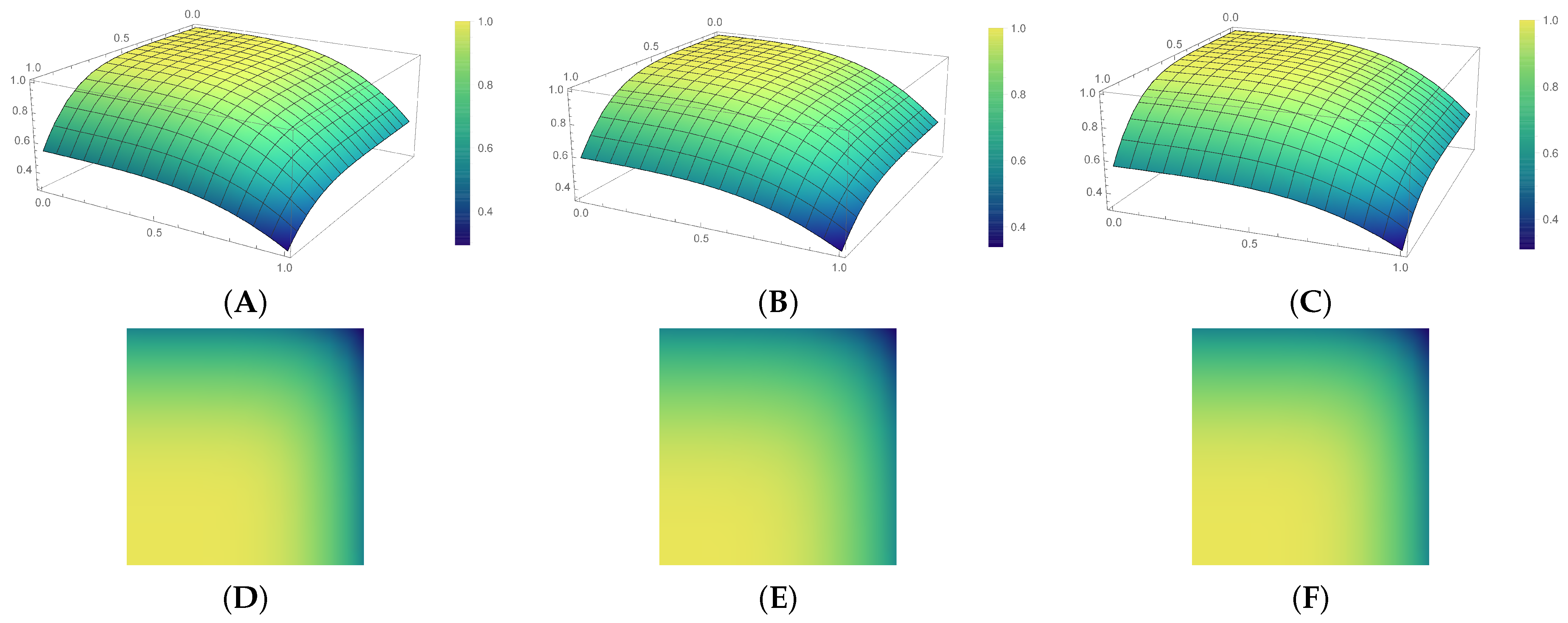
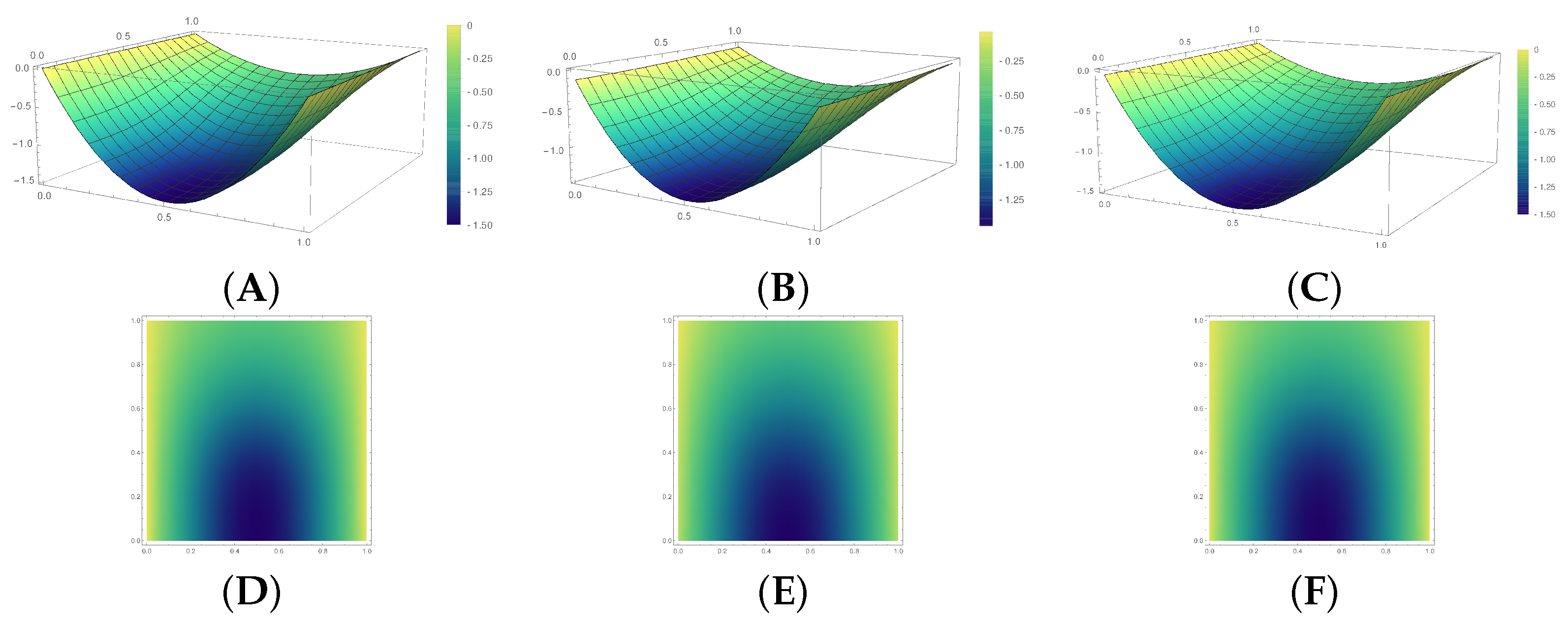
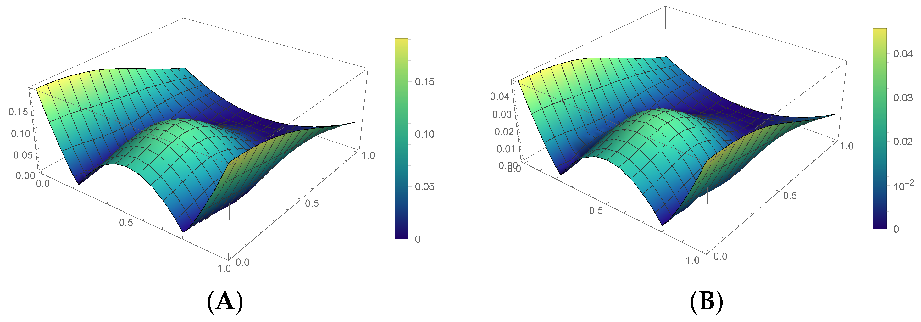
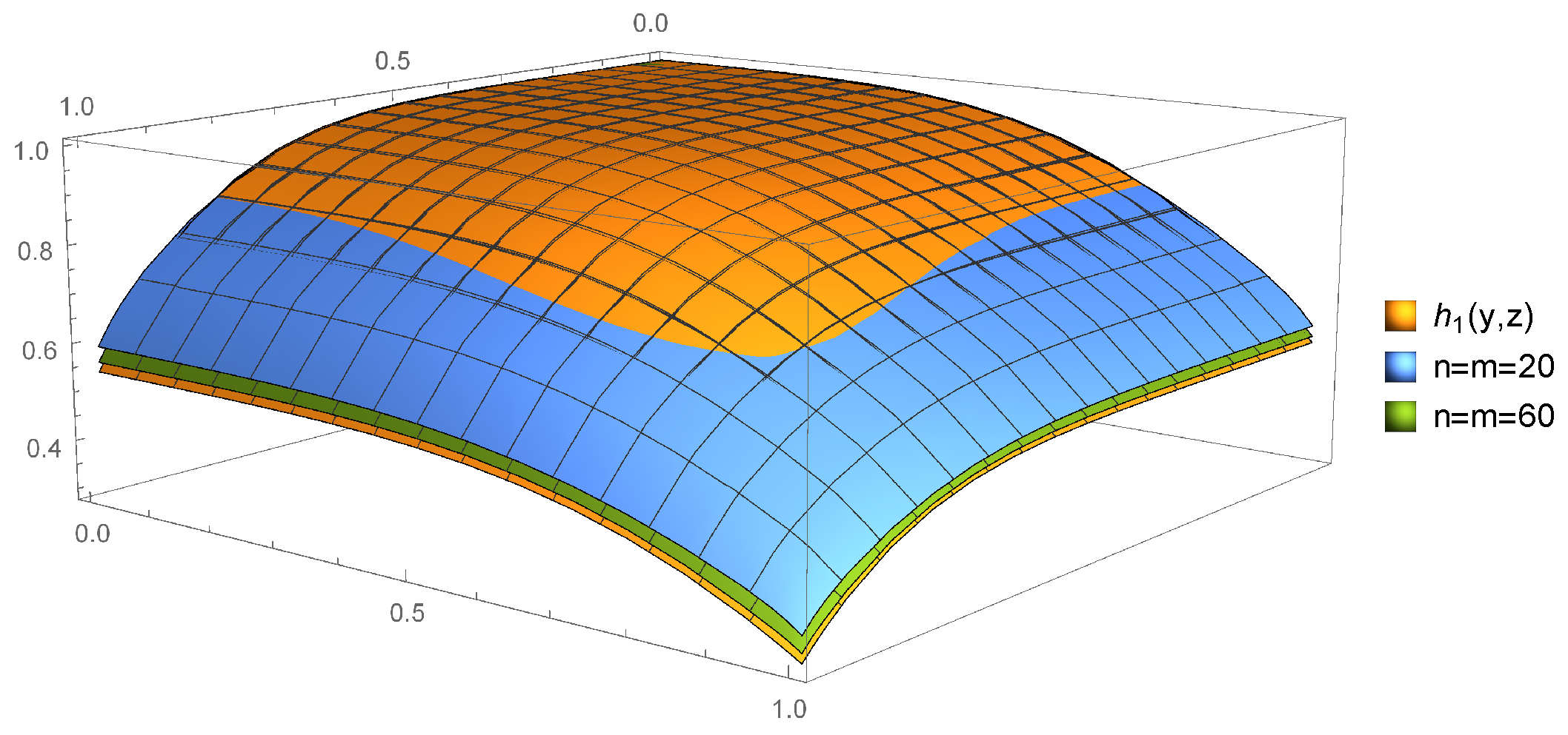
6. Numerical Results

Final section of this work provides certain numerical experiments and computer graphs supporting the theoretical results. We consider two functions for which we study approximations of our bivariate operators K r , s , κ , β γ 1 , γ 2 with them and obtain corresponding errors of approximations for different γ 1 ,   γ 2 ,   κ ,   β ,   r and s values. point represents the evaluation of the plotted function at that point. In Figure 1 and Figure 2, larger values are shown with lighter color. In Figure 1D–F and Figure 2D–F, the color of each point represents the evaluation of the plotted function at that point. In Figure 1 and Figure 2, larger values are shown with lighter color.
Example 1.
We first consider the function
h 1 ( y , z ) = cos ( y 3 ) cos ( z 2 )
on ( y , z ) [ 0 , 1 ] × [ 0 , 1 ] . Choosing γ 1 = γ 2 = 1 , κ = β = 2 we obtain some graphs to see the accuracy of the approximations for the function h 1 ( y , z ) . In Figure 3, we give three graphs; the yellow one is the graph of function h 1 ( y , z ) , the blue one is the graph for approximation of our operators when r = s = 20 , and finally the green one is also the graph for approximation of our operators when r = s = 60 . We present the graph of function h 1 ( y , z ) and approximations for r = s = 20 and r = s = 60 in Figure 1A–C, respectively. In Figure 1D–F, we give the graphs of corresponding density plots, for instance, (D) is the density plot of (A). In density plots (D)–(F), we represent the color of each corresponding point of the function. Finally we give the errors of approximations of our operators for r = s = 20 and r = s = 60 in Figure 4. It can be seen that the error decreases when the values of r and s increase, as it is expected.
Example 2.
We now consider the function
h 2 ( y , z ) = 3 y 2 3 y z 3 + 0.5
on ( y , z ) [ 0 , 1 ] × [ 0 , 1 ] . We take γ 1 = γ 2 = 0.5 , κ = β = 3 to study approximation of operators K r , s , κ , β γ 1 , γ 2 for the function h 2 ( y , z ) . We provide graph of h 2 ( y , z ) , graph for approximation of our operators when r = s = 20 , and graph for approximation of our operators when r = s = 60 in Figure 5, and we use the colors yellow, blue, and green, respectively. We give the graph of function h 1 ( y , z ) and approximations for r = s = 20 and r = s = 60 in Figure 2A–C, respectively. In Figure 2D–F, we give the corresponding density plots. Moreover, we obtain the errors of approximations when r = s = 20 and r = s = 60 in Figure 6.
As a result, we show that the operators defined in this paper approximate different kind of functions for certain γ 1 ,   γ 2 ,   κ ,   β ,   r and s values.

7. Concluding Remarks

Many mathematicians have investigated the Korovkin-type approximation theorems for a sequence of positive linear operators by different types of convergences. In this study, we focus on two summability methods including double sequences to prove Korovkin type theorems for the proposed operators. We also prove certain rates of convergence theorems connected with these two summability methods and support our theoretical results with numerical experiments. This is why the content of this paper is absolutely different from other types of papers in the literature like [9]. We also note that we reparametrize knots of operators defined in [9] and extend domain of the functions.
Now, we show that our results related to power series method are non-trivial generalization of the classical Korovkin results. Using the double sequence ϱ r , s = 1 + ( 1 ) r + s , we consider the following operators:
U r , s , κ , β γ 1 , γ 2 = ( 1 + ( 1 ) r + s ) K r , s , κ , β γ 1 , γ 2 .
We have the following results for U r , s , κ , β γ 1 , γ 2 :
U r , s , κ , β γ 1 , γ 2 ( h 0 ; y , z ) = 1 + ( 1 ) r + s , U r , s , κ , β γ 1 , γ 2 ( h 1 ; y , z ) = 1 + ( 1 ) r + s K r , s , κ , β γ 1 , γ 2 ( e 01 ; y , z ) , U r , s , κ , β γ 1 , γ 2 ( h 2 ; y , z ) = 1 + ( 1 ) r + s K r , s , κ , β γ 1 , γ 2 ( e 10 ; y , z ) , U r , s , κ , β γ 1 , γ 2 ( h 3 ; y , z ) = 1 + ( 1 ) r + s K r , s , κ , β γ 1 , γ 2 ( e 02 ; y , z ) + K r , s , κ , β γ 1 , γ 2 ( e 20 ; y , z ) .
It is clear that the operators U r , s , κ , β γ 1 , γ 2 do not satisfy Korovkin conditions for functions of two variables since U r , s , κ , β γ 1 , γ 2 ( h 0 ) = 1 + ( 1 ) r + s 1 as r , s . On the other hand, choosing R = 1 , ξ r , s = 1 and ξ ( a , b ) = 1 ( 1 a ) ( 1 b ) , we have
( 1 a ) ( 1 b ) r , s = 0 a r b s U r , s , κ , β γ 1 , γ 2 h u h u C ¯ 0 as a , b 1
for u = 0 , 1 , 2 , 3 . This means the operators U r , s , κ , β γ 1 , γ 2 converge in the sense of power series method, so Theorem 4 is valid.

Author Contributions

Methodology, F.Ö.; software, Z.Ö.Ö.; writing—original draft preparation, F.Ö.; writing—review and editing, H.M.S., K.J.A., F.Ö., Z.Ö.Ö.; visualization, Z.Ö.Ö.; supervision, H.M.S. All authors have read and agreed to the published version of the manuscript.

Funding

This research was funded by Deanship of Scientific Research at King Khalid University grant number R.G.P.1/195/42.

Acknowledgments

The authors extend their appreciation to the Deanship of Scientific Research at King Khalid University for funding this work through research groups program under Grant number R.G.P.1/195/42. The authors would like to thank to the anonymous referees for their valuable comments and efforts which definitely help to improve the quality of the paper. The authors also gratefully thank to Asif Khan, Aligarh Muslim University, India and Özer Talo, Manisa Celal Bayar University, Turkey, for their helpful comments and recommendations during the second revision of the paper.

Conflicts of Interest

The authors declare no conflict of interest.

References

  1. Weierstrass, V.K. Ueber Die Analytische Darstellbarkeit Sogennanter Willkürlicher Functionen Einer Reellen Veranderliches. Sitzungsberichte der Königlich Preußischen Akademie der Wissenschaften zu Berlin 1885, 2, 633–639. [Google Scholar]
  2. Bernstein, S.N. Démonstration du théorème de Weierstrass fondée sur le calcul des probabilités. Comm. Soc. Math. Kharkow 1912, 13, 1–2. [Google Scholar]
  3. Bernstein, S.N. Sur les recherches récentes relatives à la meilleure approximation des fonctions continues par les polynomes. In Proceedings of the fifth International Congress of Mathematicians, Cambridge, UK, 22–28 August 1912; Volume 1, pp. 256–266. [Google Scholar]
  4. Kantorovich, L. Sur Certains Developpements Suivant les Polynomes de la Forme de S. Bernstein I II Dokal Akad Nauk SSSR 1930, 563, 568. [Google Scholar]
  5. Cai, Q.B.; Lian, B.-Y.; Zhou, G. Approximation properties of λ-Bernstein operators. J. Ineq. App. 2018, 2018, 61. [Google Scholar] [CrossRef]
  6. Mohiuddine, S.A.; Özger, F. Approximation of functions by Stancu variant of Bernstein-Kantorovich operators based on shape parameter α. RACSAM 2020, 114, 70. [Google Scholar] [CrossRef]
  7. Mursaleen, M.; Ansari, K.J.; Khan, A. Some approximation results by Bernstein-Kantorovich operators based on (p,q)-calculus. U.P.B. Sci.-Bull.-Ser. A 2016, 78, 129–142. [Google Scholar]
  8. Mursaleen, M.; Ansari, K.J.; Khan, A. On (p,q)-analogue of Bernstein operators. Appl. Math. Comput. 2016, 266, 874–882, Erratum in Appl. Math. Comput. 2016, 278, 70–71. [Google Scholar] [CrossRef]
  9. Özger, F. Weighted statistical approximation properties of univariate and bivariate λ-Kantorovich operators. Filomat 2019, 33, 3473–3486. [Google Scholar] [CrossRef]
  10. Srivastava, H.M.; Özger, F.; Mohiuddine, S.A. Construction of Stancu-type Bernstein operators based on Bézier bases with shape parameter λ. Symmetry 2019, 11, 316. [Google Scholar] [CrossRef] [Green Version]
  11. Cai, Q.B. The Bézier variant of Kantorovich type λ-Bernstein operators. J. Inequal. Appl. 2018, 90. [Google Scholar] [CrossRef]
  12. Acu, A.M.; Manav, N.; Sofonea, D.F. Approximation properties of λ-Kantorovich operators. J. Inequal. Appl. 2018, 202. [Google Scholar] [CrossRef] [PubMed] [Green Version]
  13. Malkowsky, E.; Velickovic, V. Topologies of some new sequence spaces, their duals, and the graphical representation of neighbourhoods. Topol. Appl. 2011, 158, 1369–1380. [Google Scholar] [CrossRef] [Green Version]
  14. Maioa, G.D.; Kocinac, L.D.R. Statistical convergence in topology. Topol. Appl. 2008, 156, 28–45. [Google Scholar] [CrossRef] [Green Version]
  15. Pehlivan, S.; Mamedov, M.A. Statistical cluster points and turnpike. Optimization 2000, 48, 93–106. [Google Scholar] [CrossRef]
  16. Miller, H.I. A measure theoretical subsequence characterization of statistical convergence. Trans. Amer. Math. Soc. 1995, 347, 1811–1819. [Google Scholar] [CrossRef]
  17. Erdös, P.; Tenenbaur, G. Sur Les Densités de Certaines Suites D’Entiers. Proc. London Math. Soc. 1989, 59, 417–438. [Google Scholar] [CrossRef]
  18. Zygmund, A. Trigonometric Series, 2nd ed.; Cambridge University Press: Cambridge, UK, 1979. [Google Scholar]
  19. Edelya, O.H.H.; Mursaleen, M.; Khan, A. Approximation for periodic functions via weighted statistical convergence. Appl. Math. Comput. 2013, 219, 8231–8236. [Google Scholar] [CrossRef]
  20. Gadjiev, A.D.; Orhan, C. Some approximation theorems via statistical convergence. Rocky Mt. J. Math. 2002, 32, 129–138. [Google Scholar] [CrossRef]
  21. Özger, F.; Srivastava, H.M.; Mohiuddine, S.A. Approximation of functions by a new class of generalized Bernstein-Schurer operators. Rev. R. Acad. Cienc. Exactas Fís. Nat. Ser. A Math. RACSAM 2020, 114, 173. [Google Scholar] [CrossRef]
  22. Özger, F. Applications of generalized weighted statistical convergence to approximation theorems for functions of one and two variables. Numer. Funct. Anal. Optim. 2020, 41, 1990–2006. [Google Scholar] [CrossRef]
  23. Özger, F. On new Bézier bases with Schurer polynomials and corresponding results in approximation theory. Commun. Fac. Sci. Univ. Ank. Ser. A1 Math. Stat. 2019, 69, 376–393. [Google Scholar] [CrossRef]
  24. Mohiuddine, S.A.; Ahmad, N.; Özger, F.; Alotaibi, A.; Hazarika, B. Approximation by the Parametric Generalization of Baskakov-Kantorovich Operators Linking with Stancu Operators. Iran. J. Sci. Technol. Trans. Sci. 2021. [Google Scholar] [CrossRef]
  25. Alotaibi, A.; Özger, F.; Mohiuddine, S.A.; Alghamdi, M.A. Approximation of functions by a class of Durrmeyer–Stancu type operators which includes Euler’s beta function. Adv. Differ. Equ. 2021, 13. [Google Scholar] [CrossRef]
  26. Fast, H. Sur la convergence statistique. Colloq. Math. 1951, 2, 241–244. [Google Scholar] [CrossRef]
  27. Moricz, F. Statistical convergence of multiple sequences. Arch. Math. 2003, 81, 82–89. [Google Scholar] [CrossRef]
  28. Steinhaus, H. Sur la convergence ordinaire et la convergence asymptotique. Colloq. Math. 1951, 2, 73–74. [Google Scholar]
  29. Bardaro, C.; Boccuto, A.; Demirci, K.; Mantellini, I.; Orhan, S. Triangular A-statistical approximation by double sequences of positive linear operators. Results Math. 2015, 68, 271–291. [Google Scholar] [CrossRef]
  30. Demirci, K.; Orhan, S.; Kolay, B. Statistical relative A-summation process for double sequences on modular spaces. Rev. Real Acad. Cienc. Exactas Físicas Nat. Ser. A Matemáticas 2018, 112, 1249–1264. [Google Scholar] [CrossRef]
  31. Dirik, F.; Demirci, K. Korovkin type approximation theorem for functions of two variables in statistical sense. Turk. J. Math. 2010, 34, 73–83. [Google Scholar]
  32. Braha, N.L. Some properties of new modified Szász-Mirakyan operators in polynomial weight spaces via power summability methods. Bull. Math Anal. Appl. 2018, 10, 53–65. [Google Scholar]
  33. Braha, N.L. Some properties of Baskakov-Schurer-Szasz operators via power summability methods. Quaest. Math. 2019, 42, 1411–1426. [Google Scholar] [CrossRef]
  34. Braha, N.L.; Kadak, U. Approximation properties of the generalized Szasz operators by multiple Appell polynomials via power summability method. Math. Methods Appl. Sci. 2020, 43, 2337–2356. [Google Scholar] [CrossRef]
  35. Braha, N.L.; Mansour, T.; Srivastava, H.M. A parametric generalization of the Baskakov-Schurer-Szász-Stancu approximation operators. Symmetry 2021, 13, 980. [Google Scholar] [CrossRef]
  36. Söylemez, D.; Ünver, M. Korovkin type theorems for Cheney–Sharma Operators via summability methods. Results Math. 2017, 72, 1601–1612. [Google Scholar] [CrossRef]
  37. Pringsheir, A. Zur theorie der zweifach unendlichen zahlenfolges. Math. Ann. 1900, 53, 289–321. [Google Scholar] [CrossRef]
  38. Robison, G.M. Divergent double sequences and series. Amer. Math. Soc. Transl. 1926, 28, 50–73. [Google Scholar] [CrossRef]
  39. Miller, H.I. A-statistical convergence of subsequence of double sequences. Boll. U.M.I. 2007, 8, 727–739. [Google Scholar]
  40. Baron, S.; Stadtmüller, U. Tauberian theorems for power series methods applied to double sequences. J. Math. Anal. Appl. 1997, 211, 574–589. [Google Scholar] [CrossRef] [Green Version]
  41. Özger, F.; Demirci, K.; Yıldız, S. Approximation by Kantorovich Variant of λ-Schurer Operators and Related Numerical Results, Topics in Contemporary Mathematical Analysis and Applications; CRC Press: Boca Raton, FL, USA, 2020; pp. 77–94. [Google Scholar]
  42. Schurer, F. Linear Positive Operators in Approximation Theory. Ph.D. Thesis, Delft University of Technology, Delft, The Netherlands, 1962. [Google Scholar]
  43. Ye, Z.; Long, X.; Zeng, X.-M. Adjustment algorithms for Bezier curve and surface. In Proceedings of the International Conference on Computer Science and Education, Hefei, China, 24–27 August 2010; pp. 1712–1716. [Google Scholar]
  44. Demirci, K.; Yıldız, S.; Dirik, F. Approximation via power series method in two-dimensional weighted spaces. Bull. Malays. Math. Sci. Soc. 2020, 43, 3871–3883. [Google Scholar] [CrossRef]
  45. Dirik, F.; Yıldız, S.; Demirci, K. Abstract Korovkin theory for double sequences via power series method in modular spaces. Oper. Matrices 2019, 13, 1023–1034. [Google Scholar] [CrossRef] [Green Version]
  46. Ünver, M. Abel transforms of positive linear operators on weighted spaces. Bull. Belg. Math. Soc. Simon Stevin 2014, 21, 813–822. [Google Scholar] [CrossRef]
  47. Yavuz, E.; Talo, Ö. Approximation of continuous periodic functions of two variables via power series methods of summability. Bull. Malays. Math. Sci. Soc. 2019, 42, 1709–1717. [Google Scholar] [CrossRef] [Green Version]
  48. Natanson, I.P. Constructive Function Theory Volume I Uniform Approximation; Frederick Ungar Publising Company: New York, NY, USA, 1964. [Google Scholar]
Figure 1. The function h 1 ( y , z ) , and approximations for r , s = 20 and r , s = 60 with density graphs. (A) h 1 ( y , z ) ; (B) r , s = 20 ; (C) r , s = 60 ; (D) is the density plot of (A); (E) is the density plot of (B); (F) is the density plot of (C).
Mathematics 09 01895 g001
Figure 2. The function h 2 ( y , z ) , and approximations for r , s = 20 and r , s = 60 with density graphs. (A) h 2 ( y , z ) ; (B) r , s = 20 ; (C) r , s = 60 ; (D) is the density plot of (A); (E) is the density plot of (B); (F) is the density plot of (C).
Mathematics 09 01895 g002
Figure 3. Approximation with different r and s values.
Mathematics 09 01895 g003
Figure 4. Error functions for some r and s values. (A) r , s = 20 ; (B) r , s = 60 .
Mathematics 09 01895 g004
Figure 5. Approximation with different r and s values.
Mathematics 09 01895 g005
Figure 6. Error functions for some r and s values. (A) r , s = 20 ; (B) r , s = 60 .
Mathematics 09 01895 g006
Publisher’s Note: MDPI stays neutral with regard to jurisdictional claims in published maps and institutional affiliations.

