Variances and Logarithmic Aggregation Operators: Extended Tools for Decision-Making Processes

Abstract

Variance, as a measurement of dispersion, is a basic component of decision-making processes. Recent advances in intelligent systems have included the concept of variance in information fusion techniques for decision-making under uncertainty. These dispersion measures broaden the spectrum of decision makers by extending the toolset for the analysis and modeling of problems. This paper introduces some variance logarithmic averaging operators, including the variance generalized ordered weighted averaging (Var-GOWLA) operator and the induced variance generalized ordered weighted averaging (Var-IGOWLA) operator. Moreover, this paper analyzes some properties, families and particular cases of the proposed operators. Finally, an illustrative example of the characteristic design of the operators is proposed using real-world information retrieved from financial markets. The objective of this paper is to analyze the performance of some equities based on the expected payoff and the dispersion of its elements. Results show that the equity payoff results present diverse rankings combined with the proposed operators, and the introduced variance measures aid decision-making by offering new tools for information analysis. These results are particularly interesting when selecting logarithmic averaging operators for decision-making processes. The approach presented in this paper extends the available tools for decision-making under ignorance, uncertainty, and subjective environments.

1. Introduction

In statistics, variance (Var) is a fundamental descriptor of variability [1], dispersion, or spread. Variance is a measure of how data points differ from one another with respect to a specific characteristic, and each score is compared to the centermost value of the set [2]. This distinctive attribute has gained sufficient relevance in the literature such that, after the mean, variance is the second most frequently used measure to summarize the distribution of a random variable [3]. However, the calculation of variance implies squared deviations which, in some cases, are difficult to interpret and apply when considered independently. In these scenarios, the application of the squared root to the result of the variance, which is the standard deviation (SD), is suggested [4]. The SD is the most widely used measure of variability and, given its formulation, it gives more weight to larger deviations than to smaller deviations [5].

Variability measures and, in particular, variance [6], have been proven to be effective in decision-making problems. Variance measures in probabilistic feasible scenarios allow for the construction of models that aid in the assessment of a wide range of problems, including economic forecast techniques [7,8], expected utility economic issues [9], organizational management [10], risk-return organizational management [10], and risk-return organizational management analyses [11]. Variance measures are relevant in financial decision-making. For example, when an associated probability vector is included, a set of payoff setups can be constructed to aid in the selection of the most adequate option, such as in portfolio selection [12], risk premiums [13], and stock forecasting [14]. However, some real-world scenarios face problems such as a lack of information, or incomplete and subjective information. When information is not adequate for the construction of probability vectors, we need to assess decision-making problems by considering uncertainty.

In recent decades, interesting advances in the modeling of decision making in uncertainty have been made, and the seminal work of fuzzy set theory [15] has opened up new paths for the evaluation of scenarios where historic data are not available and robust mathematical techniques based on multiple valued logic are required [16]. Moreover, the decision sciences expanded [17] when the classic operation of the weighted average began to include preliminary rankings based on the attitudinal criteria of stakeholders. As a result, the ordered weighted average (OWA) operator was introduced [18]. In the literature, a wide range of aggregation operators have appeared [19], aiming to assess complex problems where different strings of information need to be included in the model. These operators include the induced OWA operator [20], the uncertain OWA operator [21], the generalized and induced generalized OWA operators [22], the ordered weighted geometric averaging operators [23], and the generalized ordered weighted logarithmic averaging operators [24].

Yager [25] proposed the study of variance as an aid for decision-making in uncertain environments. The inclusion of variability measures in decision-making problems [26] introduces new approaches for the assessment of portfolio selection problems [27], enables the possibility of selecting the alternative with the highest expected value from the range of options with the lowest inherent variance [25,28], and allows the generation of new approaches to allocate resources [29] based on minimal variance models [30] applied (for example, to personnel selection assessments) [31]. The addition of variance in the formulation of OWA operators returns a parametrized family of operators between the minimum and the maximum variance [1]. This extends decision making processes in uncertainty and offers a wider spectrum of analyzed data. These results are especially relevant in financial decision making processes where, in the case of the payoffs being equal or highly similar, an option for the selection is the one having the minimum variance [28]. The integration of variance can be widely applied in different scenarios where aggregation operators have proven to be efficient such as in economics, engineering, soft computing, the earth sciences, etc. [17,32]. Thus, the inclusion of variance in further aggregation operators is of particular interest.

Zhou and Chen [24] introduced the concept of generalized ordered weighted logarithmic aggregation (GOWLA) operators. Their proposal is based on an optimal deviation model, and its solid foundation widens the toolset for the analysis of phenomena in a variety of scenarios (for examples, see an approach to a human-resource based problem [24], financial decision making assessments [33], and multi-region decision-making problems [34]). Some developments in logarithmic averaging operators include generalized logarithmic proportional averaging operators [35], generalized ordered weighted logarithmic harmonic averaging operators [36], ordered weighted logarithmic distance operators [37], a generalized ordered weighted hybrid logarithm averaging operators [33], and continuous generalized ordered weighted logarithm aggregation operators [38]. As the family and applications of GOWLA operators continues to expand, the inclusion variance in its formulation results is interesting since it widens the study of the available data, thereby offering more information for robust decision-making approaches.

The objective of this paper is to introduce some variance logarithmic averaging operators and describe their formulation, characterization, and application. Our aim is to introduce a complementary set of tools for the assessment of decision-making problems in complex real-world scenarios when selecting logarithmic averaging operators for the aggregation of information is required. The study of variance in the logarithmic aggregation operators broadens the representation of analyzed data, giving decision makers additional information regarding the studied phenomena. This is of special interest as OWA applications continues to expand to several fields of knowledge such as in health [39], productivity [40], and social [41] and price forecasting analysis [42].

The remainder of the paper is organized as follows. Section 2 of the manuscript presents the main theories that support this study. Section 3 introduces variance ordered weighted averaging (Var-GOWLA) operators, and discusses its properties and families. Section 4 presents the induced Var-GOWLA operators, which are designed to extend the representation of the complex attitudinal character of the decision makers. Section 5 presents an illustrative example of the application of the introduced operators. Lastly, Section 6 details the concluding comments of the study.

2. Preliminaries

This section presents the basic founding tools that allow for the formulation of the proposals described in the following parts of the paper. The fundamental formulations include variance measures, the OWA operator, the reordering mechanism on the IOWA operator, and the logarithmic OWA operators.

2.1. Variance Measures

Variance is a fundamental computation of the spread of a data set. The information provided by the result of a variance calculation allows a decision maker to know whether all of the datapoints are equal (i.e., whether the variance equals zero), or whether the opposite is true when a large dissimilarity of the studied elements is observed. Among the widely disseminated definitions of variance, we can establish the following classification.

Definition 1.

The variance of a defined set of $a_i$ data elements of n magnitude is defined by the equality:

$$\mathrm{Var}\left(a_1,\dots a_n\right)={{\displaystyle \sum }}_{i=1}^n{v}_i{\left(a_i-\mu \right)}^2,$$

(1)

where all$a_i$represent argument variables. The variable$\mu$is defined as the mean (i.e.,$\mu =\frac{1}{n}{{\displaystyle \sum }}_{i=1}^n{a}_i$, and${\left(a_i-\mu \right)}^2$has an established weighting vector$v_i$), such that the sum of its elements is 1 and$v_i\in \left[0,1\right]$.

Variance is a classic measure of deviation, and its formulation allows one to understand the distribution of the data from the mean of the considered arguments. It can have applications in a plethora of fields ranging from engineering to business, machine learning, and both medical and biological sciences. From the wide range of available dispersion measures, we focus on Equation (1) (formulation of variance) since its composition allows for the description, inference, and interpretation of data, the results of which are essential for decision-making based proposals [1,25].

2.2. Ordered Weighted Average Operator

An OWA operator [18] is an information fusion technique that results in a parametric family of aggregation operators ranging from the minimum to the maximum value of the included elements. The specific allocation of weights according to its input variables has given the OWA a special relevance in the academic domain, as the applications of its design allow modeling complex settings. Please see a possible definition below.

Definition 2.

Given a weighting vector W of dimension n, characterized by $w_j\ge 0$ and ${\displaystyle \sum }{w}_j=1$, an OWA operator of dimension n is a mapping $OWA:R^n\to R$ following the next equivalence:

$$\mathrm{OWA}\left(a_1,\dots a_n\right)={{\displaystyle \sum }}_{i=1}^n{w}_i{b}_j.$$

(2)

In all cases, $b_j$ results from sorting the $a_i$ array in a descending direction.

The OWA operator can be studied and applied to various orders, such as ascending or descending orders, measures by the characterization of its weighting vector and its corresponding families, and exhibits some essential properties including commutative, monotonicity, boundedness, and idempotency.

The OWA operator is an information fusion technique [43] designed to assess multicriteria decision making and group decision making problems and rule based and fuzzy logic systems [44]. The reordering step of the OWA operator allows for the treatment of information under uncertainty [45]. In this sense, the system weights the introduced values in relation to a given order, thereby measuring the importance of the introduced values with independence to the origin of the information [46]. This characteristic design has been widely applied in automation control systems [47], computer science and information systems [48], and telecommunications [49] among a wide variety of applications. The increasing appeal of the OWA operators’ design can be observed in wide ranging reviews such as [17].

2.3. Induced Ordered Weighted Average Operator

The increasing popularity of the OWA operator’s design motivated researchers to develop new extensions and tools that allow for a wider representation of problems. Yager and Filev [20] proposed a reordering characterization of the array based on an induced mechanism. This specific reordering process allows for the distribution of weights in a particular manner, thereby adjusting to the particularities of the problem. An induced OWA operator can be described as follows:

Definition 3.

Given a weighting vector W of n dimensions delimited by $w_j\in \left[0,1\right]$ and the sum of all the included weights equal to 1, an IOWA operator of n dimensions is a mapping $IOWA:R^n\to R$, where an order-induced vector$u_i$ affects the following argument:

$$\mathrm{IOWA}\left(⟨u_1,a_1⟩,\dots ⟨u_n,a_n⟩\right)={{\displaystyle \sum }}_{i=1}^n{w}_i{b}_j.$$

(3)

The arguments here$\left(b_1,\dots b_n\right)$follow$\left(a_1,\dots ,a_n\right)$sorted by the descending values of the$u_i$array. Here,$u_i$are in fact the order-induced variables, and$a_i$ are the initial arguments.

The particularly characteristic reordering step of the induced OWA operators allows for the assessment of highly complex scenarios, bound to an intricate attitude of the decision makers, mainly in the scope of decision-making problems (see e.g., [50]) with induced OWA operators and competitive behavior variables, average induced OWA operators for the assessment of expert opinions [51], and induced OWA operators and distance measures for multi criteria group decision making problems [52].

2.4. Generalized Ordered Weighted Logarithmic Averaging Operator

Zhou and Chen [24] proposed a novel function to aggregate information based on the fundamental properties of the geometric averaging OWA operator and the result of an optimal deviation model. The introduced logarithmic operator shares some basic characteristics of the OWA operator such as monotonicity, commutativity, idempotency, and boundedness. The generalized ordered weighted logarithmic averaging (GOWLA) operators are defined as:

Definition 4.

With aspecific weighting vector W of n dimensions in ${\displaystyle \sum }{w}_j=1$and all the elements$w_j$ included in values between 0 and 1, a GOWLA operator results in a mapping GOWLA$:{\Omega }^n\to \Omega$ by the next formulation:

$$\mathrm{GOWLA}\left(a_1,\dots a_n\right)=exp\left\{{\left[{{\displaystyle \sum }}_{j=1}^n{w}_j{\left(\ln b_j\right)}^{\lambda }\right]}^{\frac{1}{\lambda }}\right\}.$$

(4)

Please observe that here$b_j$is the collection of$a_i$reordered by the largest to smallest and$a_i$ ≥ 1. Additionally, please note that λ is a parameter such that λ ∈ (− ∞, + ∞) − {0} and $\Omega =\left\{x\in R|x\ge 1\right\}$.

Further differentiations can be found in the literature for ascending and descending formulations. For example, for the OWA operator the generalized ordered weighted averaging logarithmic operator has proven to be monotonic, commutative, idempotent, and bounded (please see [24]).

The logarithmic aggregation operators have, as a foundation, an optimal deviation model, and this provides a solid theoretical basis. Its construction has been applied in multiple decision-based applications [24,33,34]. Its characteristics are interesting to furtherly explore topics such as fuzzy numbers, distance measures, and further linguistic developments.

3. Variance and Logarithmic Averaging Operators

Motivated by recent advances in the field, the present section proposes the advantages of studying logarithmic aggregation operators on variance computations. The addition of the logarithmic toolset to the variance analysis provides a wider modeling of complex phenomena, thus expanding the visualization of diverse scenarios aiding the decision-making process. These operators give the decision maker extended possibilities of results interpretation, as they complement the information portrayed by the GWLA and GOWLA operators. In the present section, the variance generalized ordered weighted logarithmic (Var-GWLA) and the variance generalized ordered weighted logarithmic averaging (Var-GOWLA) operators are proposed, including a brief description of some of their families.

3.1. Variance Generalized Weighted Averaging Operators

Following the proposal in [25], which analyzed the variance using aggregation operators, the Var-GWLA operator provided a parameterized group of ranging operators that lie between the minimum and maximum dispersion.

Definition 5.

Given a weighting vector W with characteristics $w_j\in \left[0,1\right]$and${{\displaystyle \sum }}_{j=1}^n{w}_j=1$, the Var-GWLA$\left({\sigma }^2{}_{GWLA}\right)$ operator of a population can be defined as follows:

$${\sigma }^2{}_{\mathrm{GWLA}}\left(a_1,\dots ,a_n\right)=\exp \left\{{\left[{{\displaystyle \sum }}_{j=1}^n{w}_j{\left(\ln a_j\right)}^{\mathsf{\lambda }}\right]}^{\frac{1}{\mathsf{\lambda }}}\right\},$$

(5)

where the$a_j$arguments are the result of${\left(a_i-E\right)}^2$,$a_i$is the argument variable and$E$is the resulting GWLA operator of the arguments. Additionally,$\lambda \in \left(-\infty ,+\infty \right)-\left\{0\right\}$and$a_j$≥ 1.

A direct way of obtaining the standard deviation of the ${\sigma }^2{}_{\mathrm{GWLA}}$ operator is:

$${\mathrm{SD}}_{\mathrm{GWLA}}\left(a_1,\dots ,a_n\right)=\sqrt{\exp \left\{{\left[{{\displaystyle \sum }}_{j=1}^n{w}_j{\left(\ln a_j\right)}^{\mathsf{\lambda }}\right]}^{\frac{1}{\mathsf{\lambda }}}\right\}.}$$

(6)

Example 1.

Assume the following conditions: $a_1=10,a_2=15,a_3=30,a_4=16$. If$W=\left(0.1,0.1,0.3,0.5\right)$and$\lambda =2$. Using (5) we have:

$$\begin{gathered} {\sigma }^2{}_{\mathrm{GWLA}}=\exp [{(0.1\cdot {[\ln {(10-18.7043)}^2]}^2+0.1\cdot {[\ln {(15-18.7043)}^2]}^2+0.3\cdot \\ {[\ln {(30-18.7043)}^2]}^2+0.5\cdot {[\ln {(16-18.7043)}^2]}^2)}^{1/2}]=30.1037. \end{gathered}$$

Figure 1 shows the characterization of the aggregation process with the indicated conditions in Example 1. Please note that ${\sigma }^2{}_{\mathrm{GWLA}}$ and its further generalizations and families share common properties of the logarithms. Bearing that in mind, the operator cannot carry out the aggregation process when ${\left(a_i-E\right)}^2=0$. If this is the case, this aggregation step is omitted from the general calculation and considered empty.

3.2. Variance Generalized Ordered Weighted Logarithmic Averaging Operators

When introducing an ordering mechanism, the operator changes into the Var-GOWLA $\left({\sigma }^2{}_{GOWLA}\right)$. Please note that the configuration of the ordering can be ascending or descending in the first phase. The ordering process allows the operator to run under complex scenarios, e.g., under uncertainty.

Definition 6.

A Var-GOWLA operator is defined as follows.

$${\sigma }^2{}_{\mathrm{GOWLA}}\left(a_1,\dots ,a_n\right)=\exp \left\{{\left[{{\displaystyle \sum }}_{j=1}^n{w}_j{\left(\ln R_j\right)}^{\mathsf{\lambda }}\right]}^{\frac{1}{\mathsf{\lambda }}}\right\},$$

(7)

where$R_j$is the result of${\left(b_j-\mu \right)}^2$,$b_j$are the argument variables in descending order depending on their values,$\mu$is the resulting GOWLA operator,$\lambda$is a parameter such that$\lambda \in \left(-\infty ,\infty \right)-\left\{0\right\}$, ensuring$a_j\ge 1$so that$ln{a}_j\ge 0$and$w_j\in \left[0,1\right]$also${{\displaystyle \sum }}_{j=1}^n{w}_j=1$.

The square root of the ${\sigma }^2{}_{\mathrm{GOWLA}}$ will suffice to obtain the standard deviation:

$${\mathrm{SD}}_{\mathrm{GOWLA}}\left(a_1,\dots ,a_n\right)=\sqrt{\exp \left\{{\left[{{\displaystyle \sum }}_{j=1}^n{w}_j{\left(\ln R_j\right)}^{\mathsf{\lambda }}\right]}^{\frac{1}{\mathsf{\lambda }}}\right\}}.$$

(8)

Example 2.

Continuing with the arguments presented in example 1 and using (7), we have:

$$\begin{gathered} {\sigma }^2{}_{\mathrm{GOWLA}}=\exp [{(0.1\cdot {[\ln {(30-13.5066)}^2]}^2+0.1\cdot {[\ln {(16-13.5066)}^2]}^2+ \\ 0.3\cdot {[\ln {(15-13.5066)}^2]}^2+0.5\cdot {[\ln {(10-13.5066)}^2]}^2)}^{1/2}]=13.6140. \end{gathered}$$

Figure 2 presents a plot of the resulting GOWLA and ${\sigma }^2{}_{\mathrm{GOWLA}}$ operators following the conditions established in Example 2.

The ${\sigma }^2{}_{\mathrm{GOWLA}}$ operator and its extensions share the basic property of commutativity with the OWA and the GOWLA operators, i.e., f is the ${\sigma }^2{}_{\mathrm{GOWLA}}$ operator and $b_n$ is any permutation of $a_n$, then $f\left(a_i,\dots ,a_n\right)=f\left(b_i,\dots ,b_n\right)$; however, due to the inherent characteristics of the variance, the ${\sigma }^2{}_{\mathrm{GOWLA}}$ operator does not accomplish boundedness or idempotency, and the operator is not monotonic. Figure 3 presents the general ${\sigma }^2{}_{GOWLA}$ operator behavior using the information delivered in Example 1. Please note the characteristic properties of the operator and the asymptote when reaching the GOWLA value.

3.3. Families of the Var-GOWLA

The newly introduced operator includes a λ vector that augments the model of information allowing an extended description of problems. This vector also generates several distinctive families and, in some cases, useful derivatives. For example, when the λ$\mathsf{\lambda }$ vector is equal to 1, we can apply the following definition:

Definition 7.

A variance ordered weighted logarithmic averaging operator including a W weighting vector following ${{\displaystyle \sum }}_{j=1}^n{w}_j=1$and$w_j\in \left[0,1\right]$is represented by:

$${\sigma }^2{}_{\mathrm{OWLA}}\left(a_1,\dots ,a_n\right)=\exp \left\{{{\displaystyle \sum }}_{j=1}^n{w}_j\left(\ln X_j\right)\right\},$$

(9)

where$X_j$is${\left(b_j-\mu \right)}^2$and$X_j\ge 1$, let the argument variables$X_j$be ordered in a decreasing way, and the value of$\mu$ is the resulting OWLA operator including the corresponding arguments.

Example 3.

Assume the collection of the arguments in Example 1. Using (9), we have:

$$\begin{gathered} {\sigma }^2{}_{\mathrm{OWLA}}=\exp \left[0.1\cdot \ln {\left(30-13.2115\right)}^2+0.1\cdot \ln {\left(16-13.2115\right)}^2+0.3\cdot \\ \ln {\left(15-13.2115\right)}^2+0.5\cdot \ln {\left(10-13.2115\right)}^2\right]=9.8238. \end{gathered}$$

Figure 4 presents the corresponding results of the OWLA and ${\sigma }^2{}_{\mathrm{OWLA}}$.

Table 1. Families of the Var-GOWLA operator.

λ	Operator	Formula		Acronym
$\mathsf{\lambda }\to 0$	Variance ordered weighted logarithmic geometric averaging operator	$$\begin{gathered} {\mathsf{\sigma }}^2{}_{\mathrm{OWGLA}}\left(a_1,\dots ,a_n\right) \\ =\exp \left\{{\displaystyle {\displaystyle \prod }_{j=1}^n}{\left(\ln R_j\right)}^{w_j}\right\}. \end{gathered}$$	(10)	${\mathsf{\sigma }}^2{}_{\mathrm{OWGLA}}$
$\mathsf{\lambda }=-1$	Variance ordered weighted harmonic logarithmic averaging operator	$$\begin{gathered} {\mathsf{\sigma }}^2{}_{\mathrm{OWHLA}}\left(a_1,\dots ,a_n\right) \\ =\exp \left\{\frac{1}{{{\displaystyle \sum }}_{j=1}^n\left(\frac{w_j}{\ln R_j}\right)}\right\}. \end{gathered}$$	(11)	${\mathsf{\sigma }}^2{}_{\mathrm{OWHLA}}$
$\mathsf{\lambda }=2$	Variance ordered weighted quadratic logarithmic averaging operator	$$\begin{gathered} {\mathsf{\sigma }}^2{}_{\mathrm{OWQLA}}\left(a_1,\dots ,a_n\right) \\ =\exp \left\{\sqrt[2]{{\displaystyle {\displaystyle \sum }_{j=1}^n}{w}_j{\left(\ln R_j\right)}^2}\right\}. \end{gathered}$$	(12)	${\mathsf{\sigma }}^2{}_{\mathrm{OWQLA}}$
$\mathsf{\lambda }=3$	Variance ordered weighted cubic logarithmic averaging operator	$$\begin{gathered} {\mathsf{\sigma }}^2{}_{\mathrm{OWCLA}}\left(a_1,\dots ,a_n\right) \\ =\exp \left\{\sqrt[3]{{\displaystyle {\displaystyle \sum }_{j=1}^n}{w}_j{\left(\ln R_j\right)}^3}\right\}. \end{gathered}$$	(13)	${\mathsf{\sigma }}^2{}_{\mathrm{OWCLA}}$
$\mathsf{\lambda }\to \infty$	Largest of dispersion	${\mathsf{\sigma }}^2{}_{\mathrm{GOWLA}}\left(a_1,\dots ,a_n\right)=max{R}_j$.	(14)	Max
$\mathsf{\lambda }\to -\infty$	Lowest of dispersion	${\mathsf{\sigma }}^2{}_{\mathrm{GOWLA}}\left(a_1,\dots ,a_n\right)=min{R}_j$.	(15)	Min

presents some of the most common families that can be obtained by the variation of the λ vector in the Var-GOWLA operator, including the variance ordered weighted logarithmic geometric averaging operator (Var-OWGLA), variance ordered weighted harmonic logarithmic averaging operator (Var-OWHLA), variance ordered weighted quadratic logarithmic averaging operator (Var-OWQLA), and variance ordered weighted cubic logarithmic averaging operator (Var-OWCLA), and both the largest and the lowest of the dispersion.

4. Variance Induced Ordered Weighted Logarithmic Aggregation Operators

An induced vector is an interesting tool to study when controlling the order of the aggregated arguments. In [20], the basic notion of an induced mechanism for the OWA was first introduced. Motivated by further developments, such as the induced generalized OWA operator [53] and the induced generalized ordered weighted logarithmic averaging operators [54], in this paper the variance induced ordered weighted logarithmic averaging (Var–IOWLA) operator and the variance induced generalized ordered weighted logarithmic averaging (Var–IGOWLA) operator were studied.

4.1. Variance Induced Ordered Weighted Logarithmic Averaging Operators

A Var-IOWLA operator is an extension of the Var-OWLA operator, and the main distinctive difference of this arrangement is the previous ordered induced step that allows an additional consideration of information. In this case, the previous mechanism affects the aggregation of the arguments, allowing for a wider representation of diverse phenomena.

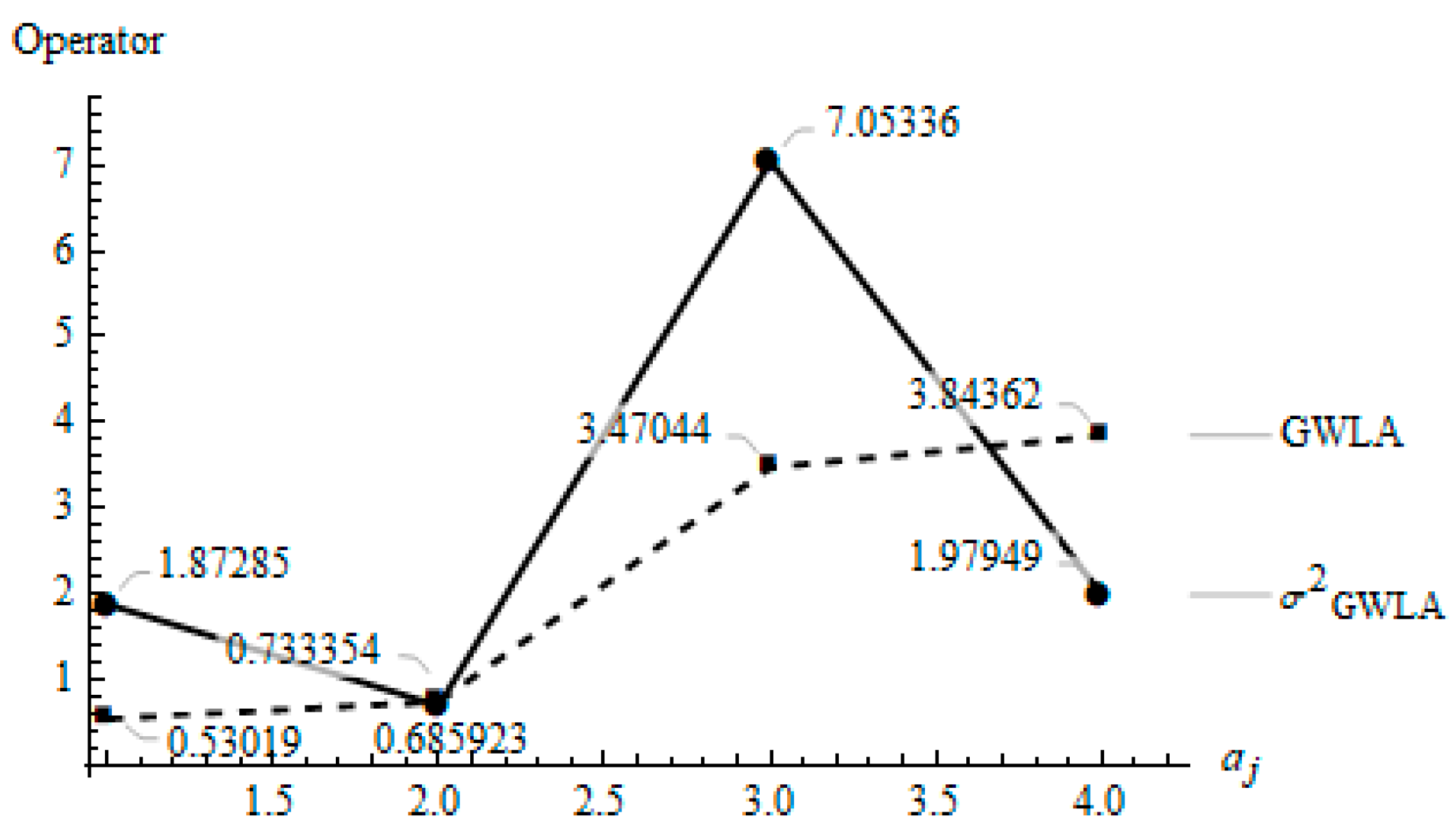
Definition 8.

This operator is defined by a characteristic weighting vector W, bounded to values between 0 and 1 such that the sum of all $w_j$ is equal to 1. The formula representing this operator is:

$${\sigma }^2{}_{\mathrm{IOWLA}}\left(⟨u_1,a_1⟩,\dots ⟨u_n,a_n⟩\right)=\exp \left\{{{\displaystyle \sum }}_{j=1}^n{w}_j\left(\ln A_j\right)\right\},$$

(16)

where$A_j$is the result of${\left(c_j-\mu \right)}^2$and$A_j\ge 1$,$c_j$is the$a_i$arguments arranged following the decreasing order of the induced set of$u_i$variables.$a_i$is the argument variables and$\mu$ is the IOWLA operator.

Example 4.

Introducing the set of conditions in Example 1 and a $U=\left(10,8,4,6\right)$ vector, using (16), we obtain:

$$\begin{gathered} {\sigma }^2{}_{\mathrm{IOWLA}}=\exp [0.1\cdot \ln {(10-20.7685)}^2+0.1\cdot \ln {(15-20.7685)}^2+0.3\cdot \\ \ln {(16-20.7685)}^2+0.5\cdot \ln {(30-20.7685)}^2]=53.8203. \end{gathered}$$

Figure 5 presents a graph of the resulting points for the IOWLA and ${\sigma }^2{}_{\mathrm{IOWLA}}$ based on the corresponding conditions.

4.2. Variance Induced Generalized Ordered Weighted Logarithmic Averaging Operators

A Var-IGOWLA operator is a generalization of the Var-IOWLA operator. The proposed difference for this case is the λ vector, which, following the proposed generalizations in the previous section, allows for the construction of wider formulations.

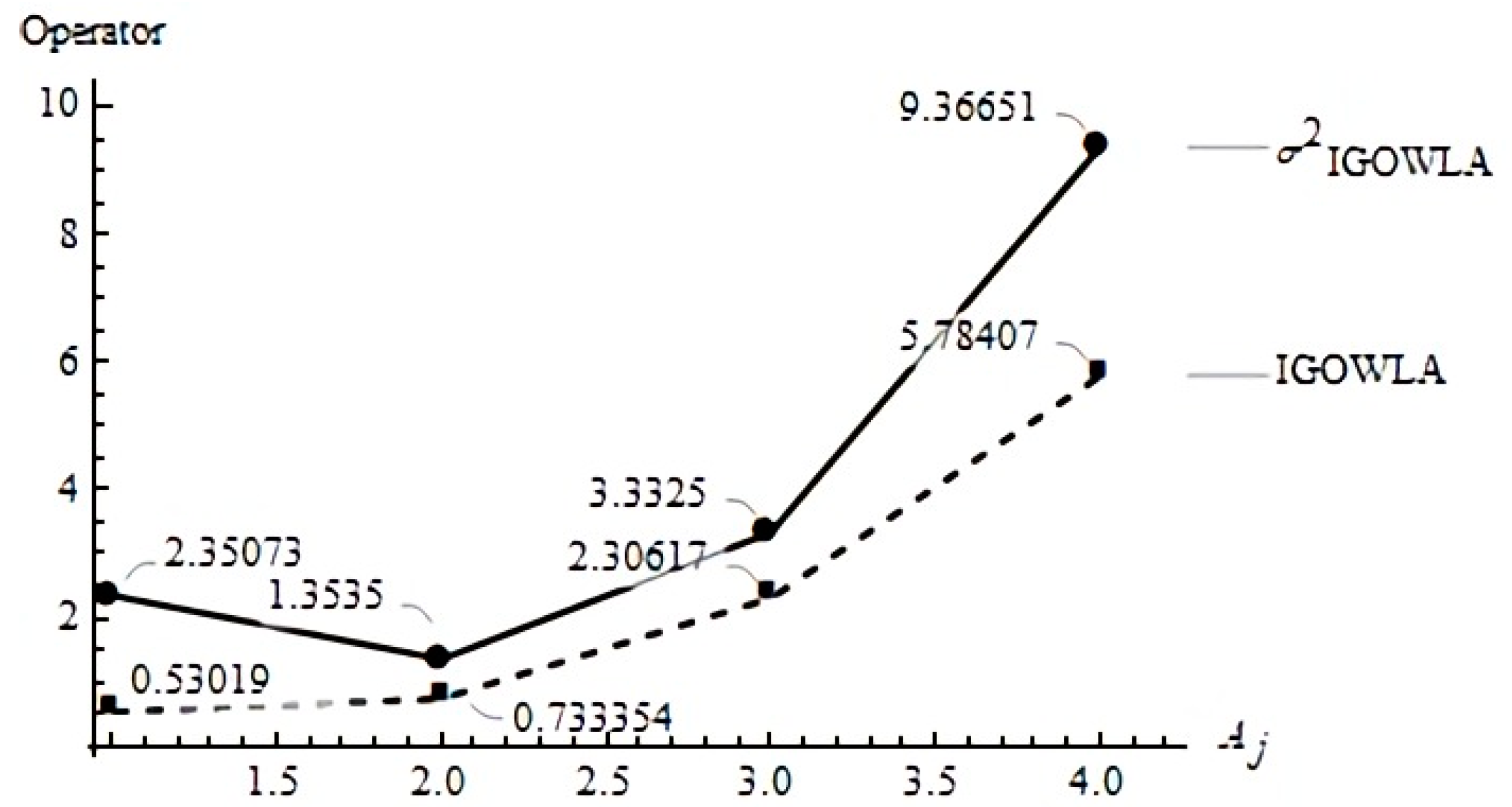
Definition 9.

A Var-IGOWLA operator with a weighting vector W, constrained to values between 0 and 1 and being the sum of all $w_j$ to 1, can be represented by:

$${\sigma }^2{}_{\mathrm{IGOWLA}}\left(⟨u_1,a_1⟩,\dots ,⟨u_n,a_n⟩\right)=\exp \left\{{\left[{{\displaystyle \sum }}_{j=1}^n{w}_j{\left(\ln X_j\right)}^{\mathsf{\lambda }}\right]}^{\frac{1}{\mathsf{\lambda }}}\right\},$$

(17)

where$X_j$is the result of${\left(c_j-\mu \right)}^2$ and$X_j\ge 1$,$c_j$is the array of$a_i$in adecreasing way dictated by the induced variables$u_i$,$a_i$is the argument variable,$\lambda \in \left(-\infty ,\infty \right)-\left\{0\right\}$and$\mu$ is the result of the corresponding IGOWLA operator.

Example 5.

Taking the arguments proposed in Example 1, an inducing vector $U=(10,8,4,6)$, and$\lambda =2$, then by using (17):

$$\begin{gathered} {\sigma }^2{}_{\mathrm{IGOWLA}}=\exp [{(0.1\cdot {[\ln {(10-21.2934)}^2]}^2+0.1\cdot {[\ln {(15-21.2934)}^2]}^2+ \\ 0.3\cdot {[\ln {(16-21.2934)}^2]}^2+0.5\cdot {[\ln {(30-21.2934)}^2]}^2)}^{1/2}]=57.4027. \end{gathered}$$

Please observe the behavior of the resulting operators following the established conditions in Figure 6.

4.3. Variance Ordered Weighted Logarithmic Averaging Operators and Quasi-Artihmetic Means

An interesting generalization of the ${\sigma }^2{}_{\mathrm{OWLA}}$ operator is the extension by quasi-arithmetic means [53,55]. These extensions allow for wider representations of problems by introducing a function describing diverse possibilities for development. In this section, we study the construction of the quasi-${\sigma }^2{}_{\mathrm{OWLA}}$ and quasi-${\sigma }^2{}_{\mathrm{IOWLA}}$ operators.

Definition 10.

A quasi-${\sigma }^2{}_{OWLA}$operator with a weighting vector W of dimension$n$is a mapping$Q{\sigma }^2{}_{OWLA}:{\Omega }^n\to \Omega$, such that${{\displaystyle \sum }}_{n=1}^j{w}_i=1$,$w_i\in \left[0,1\right]$, and a strictly monotonic continuous function$f\left(lnb\right)$, following:

$$Q{\sigma }^2{}_{\mathrm{OWLA}}\left(a_1,\dots ,a_n\right)=\exp f^{-1}\left\{{{\displaystyle \sum }}_{j=1}^n{w}_{j}f\left(\ln Z_j\right)\right\}.$$

(18)

Please observe that$Z_j$corresponds to${\left(s_j-\mu \right)}^2$, and$s_j$is the corresponding argument$a_i$ordered in a decreasing way and$\mu$is the OWLA operator calculation.

If there is a need for a customized position of the arguments to be included in the formulation, an order induced vector should be included. In this case, such representation would have as the result $Q{\sigma }^2{}_{\mathrm{IOWLA}}:{\mathsf{\Omega }}^n\to \mathsf{\Omega }$.

Definition 11.

Aquasi-${\sigma }^2{}_{IOWLA}$operator of n with dimension$n$is in fact a charting$Q{\sigma }^2{}_{OWLA}:{\Omega }^n\to \Omega$ that includes a W vector of possible weights that strictly conserves the characteristic ${{\displaystyle \sum }}_{n=1}^j{w}_i=1$, and$w_i\in \left[0,1\right]$, and a U vector of order inducing variables, such that:

$$Q{\sigma }^2{}_{\mathrm{IOWLA}}\left(⟨u_1,a_1⟩,\dots ⟨u_n,a_n⟩\right)=\exp f^{-1}\left\{{{\displaystyle \sum }}_{j=1}^n{w}_{j}f\left(\ln Z_j\right)\right\},$$

(19)

where$f$is a strictly monotonic continuous function$f\left(lnb\right)$.

As defined before, $Z_j$ is the result of ${\left(s_j-\mu \right)}^2$ with Z_j ≥ 1, and $s_j$ is the corresponding argument $a_i$ to be aggregated in a decreasing way by the decreasing influence of the $u_i$ variables; finally, $\mu$ is the IOWLA operator of the arguments.

These formulations share some interesting particular cases, such as when all the weights of the $Q{\sigma }^2{}_{\mathrm{IOWLA}}$ are the same (i.e., $\forall i\left(w_i=\frac{1}{n}\right)$), then the $Q{\sigma }^2{}_{\mathrm{IOWLA}}$ operator becomes the $Q{\sigma }^2{}_{\mathrm{IOLA}}$ quasi-variance induced ordered logarithmic averaging ${\sigma }^2{}_{\mathrm{OILA}}$ operator. If the strictly monotonic function $f\left(\ln Z_j\right)={\left(\ln Z_j\right)}^{\lambda }$, the ${\mathrm{Q}\mathsf{\sigma }}^2{}_{\mathrm{IOWLA}}$ transforms into the ${\sigma }^2{}_{\mathrm{IGOWLA}}$ operator. In the case that $f\left(\ln Z_j\right)={\left(\ln Z_j\right)}^{-1}$, we obtain the variance induced ordered weighted harmonic logarithmic averaging (${\sigma }^2{}_{\mathrm{IOWHLA}}$) operator. When $f\left(\ln Z_j\right)=\ln {\mathit{Z}}_j$, the $Q{\sigma }^2{}_{\mathrm{IGOWLA}}$ operator is simply the variance induced ordered weighted logarithmic averaging ${\sigma }^2{}_{\mathrm{IOWLA}}$ operator. Similarly, when $f\left(\ln Z_j\right)={\left(\ln Z_j\right)}^2$, the operator is the variance induced ordered weighted quadratic logarithmic averaging operator ${\sigma }^2{}_{\mathrm{IOWQLA}}$. If the function $f\left(\ln Z_j\right)={\left(\ln Z_j\right)}^3$ presents a cubic distribution, then we obtain the variance induced ordered weighted cubic logarithmic averaging (${\sigma }^2{}_{\mathrm{IOWCLA}}$) operator. In such cases that $f\left(\ln Z_j\right)={\left(\ln Z_j\right)}^{\mathsf{\lambda }}$ and $\mathsf{\lambda }\to 0$, a variance induced ordered weighted logarithmic geometric averaging ${\sigma }^2{}_{\mathrm{IOWGLA}}$ operator is produced. Finally, for $f\left(\ln Z_j\right)={\left(\ln Z_j\right)}^{\mathsf{\lambda }}$, $\mathsf{\lambda }\to \infty$ the largest and $\mathsf{\lambda }\to -\infty$, the lowest values of the dispersion are correspondingly obtained. Please note that all the particular cases mentioned above for the $Q{\sigma }^2{}_{\mathrm{IGOWLA}}$ operators are also applicable for the $Q{\sigma }^2{}_{\mathrm{GOWLA}}$ operators.

5. Variance Generalized Ordered Weighted Logarithmic Averaging Operators and Heavy Operators

In the case that a traditional bounded average (i.e., between minimum and maximum values) does not accurately represent the assessed problem, we might opt to use heavy ordered weighted averages [56]. These types of operators are often used when strong over or under estimations of the aggregation process are required.

Definition 12.

A Var-GHOWLA operator of dimension $n$is a mapping$Var-GHOWLA:{\Omega }^n\to \Omega$defined by an associate weighting vector$W$of dimension$n$such that$1\le {{\displaystyle \sum }}_{j=1}^n{w}_j\le n$and$w_j\in \left[0,1\right]$, according to the following formula:

$${\sigma }^2{}_{\mathrm{GHOWLA}}\left(a_1,\dots ,a_n\right)=\exp \left\{{\left({{\displaystyle \sum }}_{j=1}^n{w}_j{\left(\ln P_j\right)}^{\mathsf{\lambda }}\right)}^{\frac{1}{\mathsf{\lambda }}}\right\},$$

(20)

where$P_j$is the result of${\left(b_j-\mu \right)}^2$,$b_j$are the argument variables$a_i$in descending order. Here$\mu$is the resulting GOWLA operator,$\lambda$is a parameter such that$\lambda \in \left(-\infty ,\infty \right)-\left\{0\right\}$, and$a_i\ge 1$.

The distinctive difference of the Var-GHOWLA is the unbounded W weighting vector, that according to the literature [57] can further represent extreme and complex scenarios or the over estimation of the weights, due to the influence of a decision-maker.

Example 6.

Taking the arguments proposed in Example 1, $\lambda =2$, and W = (0.12, 0.14, 0.36, 0.6) then by (20):

$$\begin{gathered} {\sigma }^2{}_{\mathrm{GHOWLA}}=\exp [(0.12\cdot {[\ln {(30-17.7871)}^2]}^2+0.14\cdot {[\ln {(16-17.7871)}^2]}^2+ \\ 0.36\cdot {[\ln {(15-17.7871)}^2]}^2+0.6\cdot {[\ln {(10-17.7871)}^2]}^2{)}^{1/2}]=46.9651. \end{gathered}$$

Please observe that the W weighting vector sum is 1.22. This over representation of the weights tries to include heavily complex scenarios. Following [57], a wider representation of this overly weighted scenarios can be constructed when the heavy operator follows $-\infty \le {{\displaystyle \sum }}_{j=1}^n{w}_j\le \infty$ and $w_j\in \left[0,1\right].$

A particularity of the above-mentioned operator results when the ordering process is not carried out. In this scenario, a Var-GHWLA operator is obtained. Here, there is not a defined ordering process in the arguments. This operator follows the next formulation:

Definition 13.

A Var-GHWLA operator is an application $HOWLA:{\Omega }^n\to \Omega$of$n$dimension constituted by an associate weighting vector$W$such that$1\le {{\displaystyle \sum }}_{j=1}^n{w}_j\le n$ and $w_j\in \left[0,1\right]$, according to:

$${\sigma }^2{}_{\mathrm{GHWLA}}\left(a_1,\dots ,a_n\right)=\exp \left\{{\left({{\displaystyle \sum }}_{j=1}^n{w}_j{\left(\ln S_j\right)}^{\mathsf{\lambda }}\right)}^{\frac{1}{\mathsf{\lambda }}}\right\},$$

(21)

where$S_j$is the result of${\left(a_i-\mu \right)}^2$. Here$\mu$ is the resulting GWLA operator and $\lambda \in \left(-\infty ,\infty \right)-\left\{0\right\}$, also$a_i\ge 1$.

Example 7.

Taking the arguments proposed in Example 1, $\lambda =2$, and W = (0.12, 0.14, 0.36, 0.6) then by (21):

$$\begin{gathered} {\sigma }^2{}_{\mathrm{GHWLA}}=\exp [{(0.12\cdot {[\ln {(10-25.3067)}^2]}^2+0.14\cdot {[\ln {(15-25.3067)}^2]}^2+ \\ 0.36\cdot {[\ln {(30-25.3067)}^2]}^2+0.6\cdot {[\ln {(16-25.3067)}^2]}^2)}^{1/2}]=108.9632. \end{gathered}$$

Further representations of the heavy logarithmic variance operators can include the induced vectors. The induced values can furtherly introduce complex configurations of the aggregation operation that model the attitude of the decision makers. The induced vector forces the mechanism of the aggregation to follow a strict order. In this case, a specific representation of the induced vector can be included in the formulation.

Definition 14.

A Var-IGHOWLA operator that includes a weighting vector W, such that $1\le {{\displaystyle \sum }}_{j=1}^n{w}_j\le n$ and $w_j\in \left[0,1\right]$, is obtained by:

$${\sigma }^2{}_{\mathrm{IGHOWLA}}\left(⟨u_1,a_1⟩,\dots ⟨u_n,a_n⟩\right)=\exp \left\{{\left[{{\displaystyle \sum }}_{j=1}^n{w}_j{\left(\ln Y_j\right)}^{\mathsf{\lambda }}\right]}^{\frac{1}{\mathsf{\lambda }}}\right\},$$

(22)

where$E_j$is the result of${\left(c_j-\mu \right)}^2$ and$E_j\ge 1$,$c_j$is the set of$a_i$ following a decreasing way by the induced variables $u_i$,$a_j$are argument variables,$\lambda \in \left(-\infty ,\infty \right)-\left\{0\right\}$and$\mu$ is the result of the corresponding IGOWLA operator including the specific arguments of the aggregation.

Example 8.

Following the data proposed in Example 1, a W = (0.12, 0.14, 0.36, 0.6) and the vector $U=\left(10,8,4,6\right)$in Example 5, and$\lambda =2$, then, according to (22):

$$\begin{gathered} {\sigma }^2{}_{\mathrm{IGHOWLA}}=\exp [{(0.12\cdot {[\ln {(10-29.1403)}^2]}^2+0.14\cdot {[\ln {(15-29.1403)}^2]}^2+ \\ 0.36\cdot {[\ln {(16-29.1403)}^2]}^2+0.6\cdot {[\ln {(30-29.1403)}^2]}^2)}^{1/2}]=67.3246. \end{gathered}$$

The heavy ordered weighted averaging operators have been designed to represent widely complex real-life scenarios. These might include natural disasters, highly volatile markets, or world health issues such as pandemics. Some examples and applications are available in the literature. In incentive decision making problems [58], the heavy weighting vector aggregates the decision maker’s incentives to enlarge or shrink the expected result and heavy aggregations in enterprise risk management [59], where diverse strategies are generated, analyzed and compared, according to the decision-makers attitude.

6. Var-GOWLA Operators and the Selection of Stocks

The variance logarithmic operators have been designed to extend decision-making when using the logarithmic families of OWA operators, and the proposed mechanisms are particularly interesting when applied to finance in the selection of investment analyses in uncertain conditions. Yager [25] introduced the concept of variance to the OWA operators as a tool for analyzing not only the expected payoff of a series of options but also the variability of the alternatives. In our case, the Var-GOWLA operators serve the same purpose and widen the information that a decision maker may need to select the best option from a range of possibilities. In general, an application of the logarithmic operators, including the variance for the extension of the visualization, adheres to the following steps:

Step 1. Consider a collection of $A=\left\{A_1,A_2,\dots ,A_n\right\}$ investment stock exchange options and obtain their closing price returns for a set of $P=\left\{P_1,P_2,\dots ,P_n\right\}$ periods. These sets comprise an ${\left(x_{hi}\right)}_{m\times n}$ matrix.

Step 2. The closing price returns P require a further calculation to be fully comparable. In this case, we propose a simple calculation of the change such that $C_i=100\times \frac{\left(P_f-P_i\right)}{P_i}$. From here, a limited set of $C\in \left[1,C_n\right]$ and $C_i>0$ periods should be established, such that the analyses of the returns focus on those options that yield the largest benefit.

Step 3. The simple mean and variance are common methods for the traditional evaluation of stock performance. However, decision-making under ignorance (i.e., when the uncertainty of the assessed problem is not of a probabilistic nature or when the attitudinal characteristics of the decision makers must be included in the problem), additional tools for the appropriate assessment of financial decisions are required. For this reason, the collection of specific information from the decision maker is expected. First, a $w=\left\{w_1,w_2,\dots ,w_n\right\}$ weighting vector representing the attitudinal character with respect to the vector P is required. If the decision maker requires a specific configuration of the weighting of certain periods of time, collect an $u=\left\{u_1,u_2,\dots ,u_n\right\}$ order induced vector that correctly represents the attitudinal complexity of the phenomena.

Step 4. Solve for a selected range of operators, including the generalized ordered weighted averaging (GOWLA) operators as described in (4) and some traditional operators as the mean, and solve for the ${\mathsf{\sigma }}^2{}_{\mathrm{GOWLA}}$ operators as described in (7).

Step 5. Generate a ranking of the selected options and their results and assess a decision-making approach such that a clear selection of the chosen stock option is visualized.

Illustrative Example

The raw data included in this numerical example are retrieved from information published in the stock market for diverse assets. In the present section, we propose an illustrative example using monthly real stock data of certain equities published for Mexican companies.

Step 1. Assume that an investor would like to select the most adequate stock in which to invest. The possible set of A options include $A_1$ BIMBO A (BIMBO), $A_2$ America Movil SAB de CV (AMXL), $A_3$ ALFA A (ALFAA), $A_4$ CEMEX CPO (CEMEXCPO), $A_5$ Financiero Banorte (GFNORTEO), $A_6$ Alsea (ALSEA), $A_7$ Aeromexico (AEROMEX), and $A_8$ Herdez (HERDEZ). The selection of the stock is based on the maximum benefit with the lowest dispersion for monthly returns P during the period from January 2018 to January 2020.

Table 2. Selected stocks with monthly close return values.

Period	BIMBO	AMXL	ALFAA	CEMEXCPO	GFNORTEO	ALSEA	AEROMEX	HERDEZ
January 2020	33.81	15.69	14.14	7.60	116.09	45.76	14.26	37.49
December 2019	34.43	15.10	15.68	7.08	105.65	49.83	15.64	37.57
November 2019	33.80	15.00	15.36	7.15	102.94	52.98	15.41	38.20
October 2019	35.74	15.24	16.68	7.23	105.00	51.32	14.90	39.21
September 2019	35.99	14.64	17.33	7.69	106.07	45.88	14.37	41.82
August 2019	35.07	14.66	17.12	7.47	107.82	42.74	15.26	41.78
July 2019	36.50	13.48	16.60	6.81	96.48	39.07	15.08	40.11
June 2019	40.03	13.97	18.86	8.09	111.36	37.78	18.16	41.13
May 2019	39.55	13.79	17.89	7.99	106.59	38.29	17.89	40.15
April 2019	42.22	14.12	19.16	8.77	119.83	42.38	19.43	40.63
March 2019	40.58	13.88	20.63	9.07	105.54	40.67	20.48	43.30
February 2019	38.23	13.88	21.95	9.46	104.85	48.81	20.82	42.71
January 2019	37.81	15.31	24.07	10.33	106.16	52.92	24.32	41.75
December 2018	39.15	13.97	23.38	9.49	95.78	51.15	22.20	41.00
November 2018	39.00	13.68	20.46	10.47	93.15	51.01	21.69	41.79
October 2018	38.05	14.71	21.41	10.14	111.76	51.94	22.41	37.74
September 2018	39.91	15.04	24.13	13.14	135.30	63.67	25.69	42.33
August 2018	39.75	16.05	25.13	13.53	130.86	68.06	26.86	41.15
July 2018	39.66	15.97	25.36	13.89	129.96	64.29	28.55	40.49
June 2018	38.69	16.57	23.10	13.06	117.07	68.40	26.99	41.86
May 2018	38.06	15.50	20.48	11.86	106.20	65.41	24.35	39.43
April 2018	43.53	17.31	24.01	11.70	117.02	69.56	26.15	44.77
March 2018	39.78	17.25	23.29	12.03	111.13	63.53	29.00	45.99
February 2018	44.11	17.34	22.39	12.45	113.16	64.26	29.20	46.19
January 2018	45.40	17.44	23.36	15.48	119.58	60.88	29.53	43.68
December 2017	43.51	16.95	21.62	14.70	107.83	64.37	28.59	45.68

Source: Mexican market equities historic data retrieved from the website https://mx.investing.com/equities/ (accessed on 22 July 2021). All of the values are in MXN.

presents the monthly close returns ${\left(x_{hi}\right)}_{m\times n}$ matrix of the selected companies for the corresponding period.

Step 2. The decision maker will make the final selection based on the maximum benefit with the lowest dispersion for C = 10 periods of positive yields of the selected stocks.

Table 3. Selected positive return periods to be considered.

$\mathit{C}$	BIMBO	AMXL	ALFAA	CEMEXCPO	GFNORTEO	ALSEA	AEROMEX	HERDEZ
$C_1$	1.86	3.91	2.08	7.34	9.88	3.23	1.49	0.10
$C_2$	2.62	0.67	1.23	2.95	2.63	11.86	3.42	4.16
$C_3$	1.21	4.10	3.13	9.69	11.75	7.35	3.69	2.44
$C_4$	4.04	8.75	5.42	1.25	4.48	9.39	1.19	1.38
$C_5$	6.15	1.31	2.95	8.85	13.54	3.41	1.51	2.30
$C_6$	1.11	1.73	14.27	3.25	0.66	4.20	9.55	1.83
$C_7$	0.38	9.59	9.78	6.36	10.84	3.46	2.35	10.73
$C_8$	2.50	2.12	12.79	10.12	2.82	0.27	5.78	2.87
$C_9$	0.40	0.50	3.09	1.37	3.39	5.86	10.84	1.63
$C_{10}$	0.23	6.90	4.02	5.31	0.69	4.57	3.29	6.16

includes the corresponding C periods to be analyzed.

Step 3. A W weighting vector of W (0.25, 0.23, 0.1, 0.09, 0.08, 0.07, 0.06, 0.05, 0.04, 0.03) for the representation of the attitudinal characteristic of the decision maker is included. Please note that this is a rather optimistic orientation. Furthermore, the decision maker would like to include an additional perspective to the problem, in this case the optimistic characterization for some specific months of the year. For this, we include an induced weighting vector of U (10, 9, 8, 1, 2, 3, 4, 5, 6, 7).

Step 4. With these set values, we can now solve for GOWLA and ${\sigma }^2{}_{\mathrm{GOWLA}}$ operators and contrast the results with those of certain traditional and other uncertainty-oriented proposed methods.

Table 4. Payoff aggregated results.

Operator	BIMBO	AMXL	ALFAA	CEMEXCPO	GFNORTEO	ALSEA	AEROMEX	HERDEZ
AVG	2.05	3.96	5.88	5.65	6.07	5.36	4.31	3.36
OWA	3.30	6.14	8.97	7.62	9.01	7.56	6.63	5.38
GOWLA	2.45	4.74	7.24	6.73	7.04	6.41	5.38	3.98
IGOWLA	1.95	3.85	6.44	5.63	5.52	5.24	4.79	3.15
GOWQLA	3.57	5.89	8.23	7.34	8.42	7.32	6.21	5.31
IGOWQLA	3.74	5.61	7.79	6.62	7.65	7.08	5.90	5.68
GOWCLA	3.62	6.43	9.00	7.72	9.12	7.61	6.82	5.43
IGOWCLA	3.40	6.24	8.76	7.23	8.58	7.26	6.67	4.87

shows the resulting payoff of the selected stocks based on the GOWLA operator and certain other methods.

Table 5. Dispersion aggregated results.

Operator	BIMBO	AMXL	ALFAA	CEMEXCPO	GFNORTEO	ALSEA	AEROMEX	HERDEZ
${\sigma }^2$	3.52	11.29	21.90	11.20	23.96	11.38	11.54	9.44
${\sigma }^2\mathrm{OWA}$	4.06	11.00	23.51	8.23	20.31	11.36	13.20	12.31
${\sigma }^2\mathrm{GOWLA}$	1.14	7.86	20.05	4.87	20.41	6.54	8.09	4.34
${\sigma }^2\mathrm{IGOWLA}$	2.51	8.94	23.69	9.61	24.26	9.44	10.83	5.98
${\sigma }^2\mathrm{GOWQLA}$	4.96	9.84	21.45	62.50	17.51	26.62	12.95	9.80
${\sigma }^2\mathrm{IGOWQLA}$	7.37	12.39	25.26	11.61	24.06	13.86	19.40	12.90
${\sigma }^2\mathrm{GOWCLA}$	4.13	10.57	22.50	7.61	18.38	9.85	12.97	12.08
${\sigma }^2\mathrm{IGOWCLA}$	5.51	13.32	25.92	9.93	23.88	6.38	15.05	13.26

presents the resulting aggregation of the dispersion based on the proposed ${\sigma }^2{}_{\mathrm{GOWLA}}$ operators.

Step 5. The decision of selecting an asset could be given by the highest payoff, the lowest dispersion of the data, or a combination of both.

Table 6. Ranking based on highest payoff.

Operator	Preference
AVG	GFNORTEO ≻ ALFAA ≻ CEMEXCPO ≻ ALSEA ≻ AEROMEX ≻ AMXL ≻ HERDEZ ≻ BIMBO
OWA	GFNORTEO ≻ ALFAA ≻ CEMEXCPO ≻ ALSEA ≻ AEROMEX ≻ AMXL ≻ HERDEZ ≻ BIMBO
GOWLA	ALFAA ≻ GFNORTEO ≻ CEMEXCPO ≻ ALSEA ≻ AEROMEX ≻ AMXL ≻ HERDEZ ≻ BIMBO
GOWQLA	GFNORTEO ≻ ALFAA ≻ CEMEXCPO ≻ ALSEA ≻ AEROMEX ≻ AMXL ≻ HERDEZ ≻ BIMBO
GOWCLA	GFNORTEO ≻ ALFAA ≻ CEMEXCPO ≻ ALSEA ≻ AEROMEX ≻ AMXL ≻ HERDEZ ≻ BIMBO
IGOWLA	ALFAA ≻ CEMEXCPO ≻ GFNORTEO ≻ ALSEA ≻ AEROMEX ≻ AMXL ≻ HERDEZ ≻ BIMBO
IGOWQLA	ALFAA ≻ GFNORTEO ≻ ALSEA ≻ CEMEXCPO ≻ AEROMEX ≻ HERDEZ ≻ AMXL ≻ BIMBO
IGOWCLA	ALFAA ≻ GFNORTEO ≻ ALSEA ≻ CEMEXCPO ≻ AEROMEX ≻ AMXL ≻ HERDEZ ≻ BIMBO

presents the ranking of the selected stocks depending on the highest payoff.

Table 7. Ranking based on lowest dispersion.

Operator	Preference
${\sigma }^2$	BIMBO ≻ HERDEZ ≻ CEMEXCPO ≻ AMXL ≻ ALSEA ≻ AEROMEX ≻ ALFAA≻ GFNORTEO
${\sigma }^2\mathrm{OWA}$	BIMBO ≻ CEMEXCPO ≻ AMXL ≻ ALSEA ≻ HERDEZ ≻ AEROMEX ≻ GFNORTEO ≻ ALFAA
${\sigma }^2\mathrm{GOWLA}$	BIMBO ≻ HERDEZ ≻ CEMEXCPO ≻ ALSEA ≻ AMXL ≻ AEROMEX ≻ ALFAA ≻ GFNORTEO
${\sigma }^2\mathrm{GOWQLA}$	BIMBO ≻ HERDEZ ≻ AMXL ≻ AEROMEX ≻ GFNORTEO ≻ ALFAA ≻ ALSEA ≻ CEMEXCPO
${\sigma }^2\mathrm{GOWCLA}$	BIMBO ≻ CEMEXCPO ≻ ALSEA ≻ AMXL ≻ HERDEZ ≻ AEROMEX ≻ GFNORTEO ≻ ALFAA
${\sigma }^2\mathrm{IGOWLA}$	BIMBO ≻ HERDEZ ≻ AMXL ≻ ALSEA ≻ CEMEXCPO ≻ AEROMEX ≻ ALFAA ≻ GFNORTEO
${\sigma }^2\mathrm{IGOWQLA}$	BIMBO ≻ CEMEXCPO ≻ AMXL ≻ HERDEZ ≻ ALSEA ≻ AEROMEX ≻ GFNORTEO ≻ ALFAA
${\sigma }^2\mathrm{IGOWCLA}$	BIMBO ≻ ALSEA ≻ CEMEXCPO ≻ HERDEZ ≻ AMXL ≻ AEROMEX ≻ GFNORTEO ≻ ALFAA

shows the ranking of the stocks by the minimum dispersion of their information.

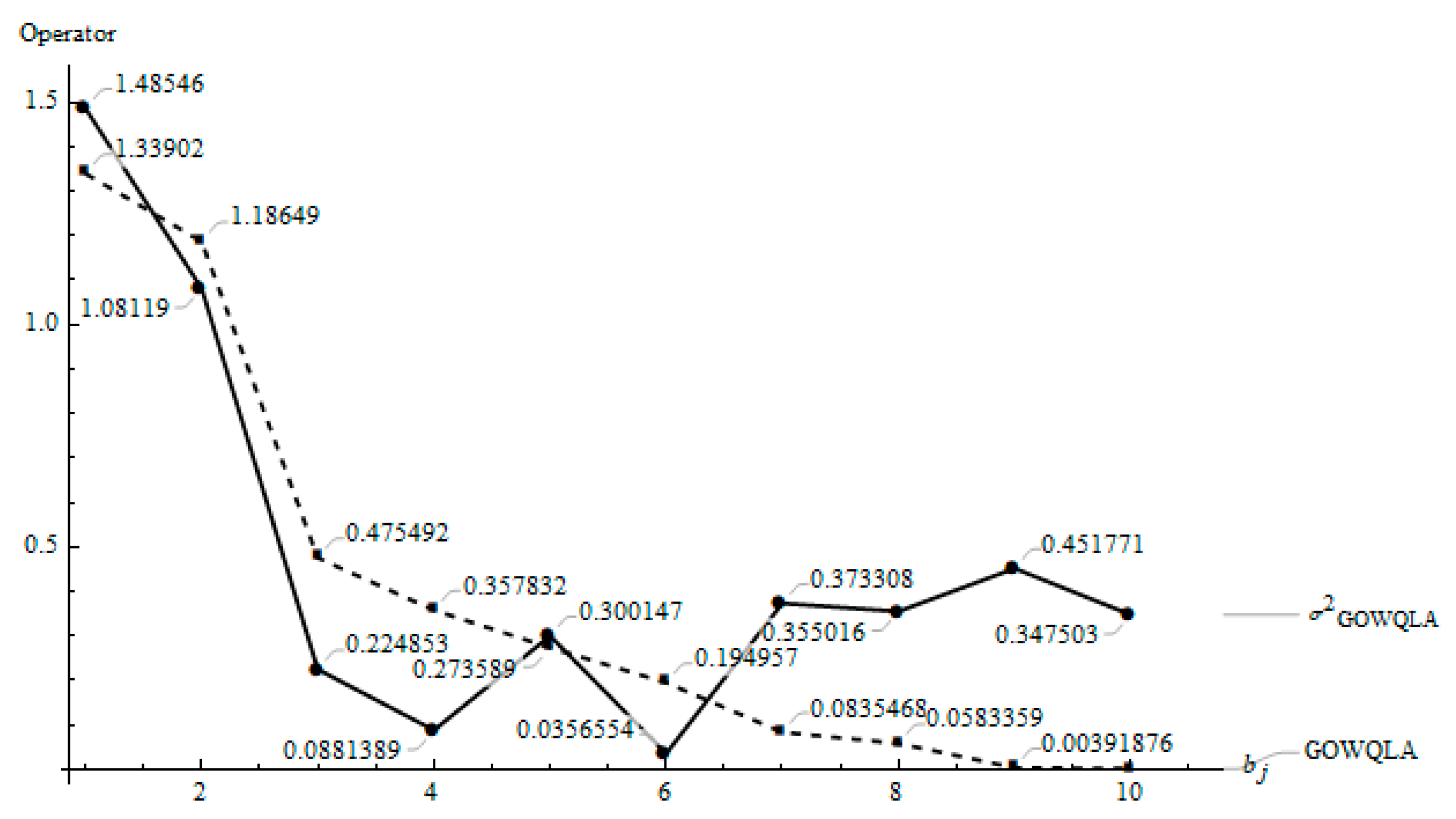
The results vary depending on the operator utilized for the analysis. However, some operators match in the ranking of the selected equities. When analyzing the payoffs of the selected stocks in combination with their variance, the results vary significantly. In general, the stock with the highest payoff is given by either GFNORTEO or ALFAA. However, the dispersion of these stocks is the highest, resulting in these stocks being the last position of the ranking for the majority of the operators. When selecting a stock, low dispersion is preferred. Therefore, the decision should include the results of the lowest variance, and depending on the operator selected, this can vary over diverse options. If both criteria are considered and the GOWLA operator is considered, then CEMEXCPO is the selected option for the conditions established. Please observe the generated plot for CEMEXCPO analyzed with the GOWQLA and ${\mathsf{\sigma }}^2{}_{\mathrm{GOWQLA}}$ operators in Figure 7.

7. Conclusions

In this paper we have analyzed some variance logarithmic averaging operators. Variance is one of the most common dispersion measures and has been included as part of the ordered weighted average operators’ toolset since 1996. Some of the advantages of including variance as a dispersion measure in OWA operators include the additional information given to decision makers to generate informed choices between diverse alternatives. The benefits of using the logarithmic averaging operators and the introduced variance dispersion measures are wider representation of complex problems, the ability to consider the attitudinal characters of the decision makers, the logarithmic properties of the operators, and the wide-ranging set of configurations that the proposed generalizations allow.

In general, two families of variance aggregation operators are proposed, the variance generalized ordered weighted averaging $({\sigma }^2{}_{\mathrm{GOWLA}}$) operators and the induced variance ordered weighted averaging (${\sigma }^2{}_{\mathrm{IGOWLA}})$ operators. The Var-GOWLA is a proposition based on the optimal deviation model introduced by [24] and the inclusion of dispersion measures developed by [25]. Here, its properties, particular cases, and some families are studied. Moreover, the Var-IGOWLA operator is also introduced. In this case, the ordering of the elements depends on the included inducing vector, which allows wider representations of diverse problems and, specifically, the customization of the analyses depending on the decision maker’s points of view.

The introduced variance tools in the logarithmic averaging operators are designed to extend the decision-making process by allowing the possibility of having an additional measure to model a specific problem. The characteristic design of the ${\mathsf{\sigma }}^2\mathrm{GOWLA}$ and the ${\mathsf{\sigma }}^2\mathrm{IGOWLA}$ operators can be applied to a variety of problems in engineering, statistics, and economics. However, it is particularly interesting in financial decision-making. In this paper, an illustrative example including real-world financial information is proposed. This case analyses eight equities from the Mexican financial markets. The monthly closing price for ten positive return months is retrieved and analyzed with traditional, ordered weighted averaging operators and logarithmic averaging operators, and this analysis includes its dispersion measures. The objective, here, is to rank the performance of the equities based on the expected payoff of the identified data points and its dispersion. The results conclude that the payoff ranking is equal to some studies’ equities. However, the dispersion measures show varying results, depending on the operator utilized.

This paper studies extended tools for decision-making under ignorance and uncertainty and when subjective information or the attitudinal characters of stakeholders must be modeled. The implications of this research can directly improve decision-making when using a combined view of the logarithmic averaging operators and introducing dispersion measures. Further research is required, especially to strengthen the benefits of the logarithmic properties of the introduced operators, the specifications that result in the most appropriate selection of these operators [60], and the inclusion of the variance and other modeling tools including fuzzy and interval numbers, distances, and Bonferroni approaches (among other models).

References

1. Blanco-Mesa, F.; León-Castro, E.; Merigó, J.M.; Herrera-Viedma, E. Variances with Bonferroni means and ordered weighted averages. Int. J. Intell. Syst. 2019, 34, 3020–3045. [Google Scholar] [CrossRef]
2. Soong, T.T. Fundamentals of Probability and Statistics for Engineers; Wiley: Hoboken, NJ, USA, 2014. [Google Scholar]
3. Montgomery, D.C.; Runger, G.C. Applied Statistics and Probability for Engineers, 6th ed.; Wiley: Hoboken, NJ, USA, 2014. [Google Scholar]
4. Black, K. Business Statistics for Contemporary Decision Making, 6th ed.; Wiley: Hoboken, NJ, USA, 2010. [Google Scholar]
5. De Coursey, W.J. Statistics and Probability for Engineering Applications; Elsevier Science: Woburn, MA, USA, 2003. [Google Scholar]
6. Fisher, R.A. The correlation between relatives on the supposition of mendelian inheritance. Trans. R. Soc. Edinb. 1919, 52, 399–433. [Google Scholar] [CrossRef] [Green Version]
7. Brailsford, T.J.; Faff, R.W. An evaluation of volatility forecasting techniques. J. Bank. Financ. 1996, 20, 419–438. [Google Scholar] [CrossRef]
8. Verma, R.; Merigó, J.M. Variance measures with ordered weighted aggregation operators. Int. J. Intell. Syst. 2019, 34, 1184–1205. [Google Scholar] [CrossRef]
9. Siniscalchi, M. Vector expected utility and attitudes toward variation. Econometrica 2009, 77, 801–855. [Google Scholar] [CrossRef] [Green Version]
10. Thatcher, S.M.B.; Patel, P.C. Group Faultlines: A review, integration, and guide to future research. J. Manag. 2012, 38, 969–1009. [Google Scholar] [CrossRef]
11. McNamara, G.; Bromiley, P. Risk and return in organizational decision making. Acad. Manag. J. 1999, 42, 330–339. [Google Scholar]
12. Li, D.; Ng, W.-L. Optimal dynamic portfolio selection: Multiperiod mean-variance formulation. Math. Financ. 2000, 10, 387–406. [Google Scholar] [CrossRef]
13. Carr, P.; Wu, L. Variance Risk Premiums. Rev. Financ. Stud. 2009, 22, 1311–1341. [Google Scholar] [CrossRef]
14. Lamoureux, C.G.; Lastrapes, W.D. Forecasting stock-return variance: Toward an understanding of stochastic implied olatilities. Rev. Financ. Stud. 1993, 6, 293–326. [Google Scholar] [CrossRef]
15. Zadeh, L.A. Fuzzy sets. Inf. Control 1965, 8, 338–353. [Google Scholar] [CrossRef] [Green Version]
16. Kacprzyk, J.; Yager, R.R.; Merigó, J.M. Towards Human-Centric Aggregation via Ordered Weighted Aggregation Operators and Linguistic Data Summaries: A New Perspective on Zadeh’s Inspirations. IEEE Comput. Intell. Mag. 2019, 14, 16–30. [Google Scholar] [CrossRef]
17. Blanco-Mesa, F.; León-Castro, E.; Merigó, J.M. A bibliometric analysis of aggregation operators. Appl. Soft Comput. 2019, 81, 105488. [Google Scholar] [CrossRef]
18. Yager, R.R. On ordered weighted averaging aggregation operators in multicriteria decisionmaking. IEEE Trans. Syst. Man Cybern. 1988, 18, 183–190. [Google Scholar] [CrossRef]
19. Emrouznejad, A.; Marra, M. Ordered weighted averaging operators 1988–2014: A citation-based literature survey. Int. J. Intell. Syst. 2014, 29, 994–1014. [Google Scholar] [CrossRef] [Green Version]
20. Yager, R.R.; Filev, D.P. Induced ordered weighted averaging operators. IEEE Trans. Syst. Man Cybern. Part B Cybern. 1999, 29, 141–150. [Google Scholar] [CrossRef] [PubMed]
21. Xu, Z.S.; Da, Q.L. The uncertain OWA operator. Int. J. Intell. Syst. 2002, 17, 569–575. [Google Scholar] [CrossRef]
22. Yager, R.R. Generalized OWA Aggregation Operators. Fuzzy Optim. Decis. Mak. 2004, 3, 93–107. [Google Scholar] [CrossRef]
23. Xu, Z.S.; Da, Q.L. The ordered weighted geometric averaging operators. Int. J. Intell. Syst. 2002, 17, 709–716. [Google Scholar] [CrossRef]
24. Zhou, L.; Chen, H. Generalized ordered weighted logarithm aggregation operators and their applications to group decision making. Int. J. Intell. Syst. 2010, 25, 683–707. [Google Scholar] [CrossRef]
25. Yager, R.R. On the inclusion of variance in decision making under uncertainty. Int. J. Uncertain. Fuzziness Knowl. Based Syst. 1996, 4, 401–419. [Google Scholar] [CrossRef]
26. Merigó, J.M.; Guillén, M.; Sarabia, J.M. The Ordered Weighted Average in the Variance and the Covariance. Int. J. Intell. Syst. 2015, 30, 985–1005. [Google Scholar] [CrossRef]
27. Laengle, S.; Loyola, G.; Merigó, J.M. Mean-Variance portfolio selection with the ordered weighted average. IEEE Trans. Fuzzy Syst. 2017, 25, 350–362. [Google Scholar] [CrossRef]
28. Yager, R.R. Generalizing variance to allow the inclusion of decision attitude in decision making under uncertainty. Int. J. Approx. Reason. 2006, 42, 137–158. [Google Scholar] [CrossRef] [Green Version]
29. Chang, K.-H. A more general reliability allocation method using the hesitant fuzzy linguistic term set and minimal variance OWGA weights. Appl. Soft Comput. 2017, 56, 589–596. [Google Scholar] [CrossRef]
30. Liu, X. The solution equivalence of minimax disparity and minimum variance problems for OWA operators. Int. J. Approx. Reason. 2007, 45, 68–81. [Google Scholar] [CrossRef] [Green Version]
31. Wen, T.-C.; Chang, K.-H.; Lai, H.-H. Improving personnel selection by combining the minimal variance OWA operator and IPA. J. Intell. Fuzzy Syst. 2018, 35, 6229–6239. [Google Scholar] [CrossRef]
32. Yu, D.; Wang, W.; Zhang, W.; Zhang, S. A bibliometric analysis of research on multiple criteria decision making. Curr. Sci. 2018, 114, 747. [Google Scholar] [CrossRef]
33. Liu, J.P.; Chen, H.Y.; Zhou, L.G.; Tao, Z. Generalized linguistic ordered weighted hybrid logarithm averaging operators and applications to group decision making. Int. J. Uncertain. Fuzziness Knowl. Based Syst. 2015, 23, 421–442. [Google Scholar] [CrossRef]
34. Alfaro-García, V.G.; Merigó, J.M.; Plata-Pérez, L.; Alfaro-Calderón, G.G.; Gil-Lafuente, A.M. Induced and logarithmic distances with multi-region aggregation operators. Technol. Econ. Dev. Econ. 2019, 25, 1–29. [Google Scholar] [CrossRef]
35. Zhou, L.G.; Chen, H.Y.; Liu, J.P. Generalized logarithmic proportional averaging operators and their applications to group decision making. Knowl. Based Syst. 2012, 36, 268–279. [Google Scholar] [CrossRef]
36. Zhou, L.G.; Tao, Z.F.; Chen, H.Y.; Liu, J.P. Generalized ordered weighted logarithmic harmonic averaging operators and their applications to group decision making. Soft Comput. 2015, 19, 715–730. [Google Scholar] [CrossRef]
37. Alfaro-García, V.G.; Merigó, J.M.; Gil-Lafuente, A.M.; Kacprzyk, J. Logarithmic aggregation operators and distance measures. Int. J. Intell. Syst. 2018, 33, 1488–1506. [Google Scholar] [CrossRef] [Green Version]
38. Liu, J.; Lin, S.; Chen, H.; Zhou, L. The continuous quasi-OWA operator and its application to group decision making. Gr. Decis. Negot. 2013, 22, 715–738. [Google Scholar] [CrossRef]
39. Brotons-Martínez, J.M.; Sansalvador-Sellés, M.E. Proposal for a fuzzy model to assess cost overrun in healthcare due to delays in treatment. Mathematics 2021, 9, 408. [Google Scholar] [CrossRef]
40. Chiu, M.C.; Chen, T.C.T.; Hsu, K.W. Modeling an uncertain productivity learning process using an interval fuzzy methodology. Mathematics 2020, 8, 998. [Google Scholar] [CrossRef]
41. Perez-Arellano, L.A.; Blanco-Mesa, F.; Leon-Castro, E.; Alfaro-Garcia, V. Bonferroni prioritized aggregation operators applied to government transparency. Mathematics 2020, 9, 24. [Google Scholar] [CrossRef]
42. Espinoza-Audelo, L.F.; Olazabal-Lugo, M.; Blanco-Mesa, F.; León-Castro, E.; Alfaro-Garcia, V. Bonferroni probabilistic ordered weighted averaging operators applied to agricultural commodities’ price analysis. Mathematics 2020, 8, 1350. [Google Scholar] [CrossRef]
43. Beliakov, G.; Sola, H.B.; Sánchez, T.C. A Practical Guide to Averaging Functions; Springer: Berlin/Heidelberg, Germany, 2016. [Google Scholar]
44. Beliakov, G.; Pradera, A.; Calvo, T. Aggregation Functions: A Guide for Practitioners; Studies in Fuzziness and Soft Computing; Springer: Berlin/Heidelberg, Germany, 2007; Volume 221, ISBN 978-3-540-73720-9. [Google Scholar]
45. Yager, R.R.; Kacprzyk, J. (Eds.) The Ordered Weighted Averaging Operators; Springer: Boston, MA, USA, 1997; ISBN 978-1-4613-7806-8. [Google Scholar]
46. Torra, V. The weighted OWA operator. Int. J. Intell. Syst. 1997, 12, 153–166. [Google Scholar] [CrossRef]
47. Xu, M.; Fu, H.; Tian, W.; Lyu, B.; Jiang, Z.; Guan, B. Reliability allocation of rotary ultrasonic vibration-assisted EDM machine tool based on maximum entropy ordered weighted average and constraint under the index of overall cost. Int. J. Adv. Manuf. Technol. 2021, 1–10. [Google Scholar] [CrossRef]
48. Fourour, S.; Lebbah, Y. Equitable optimization for multicast communication. Int. J. Decis. Support Syst. Technol. 2020, 12, 1–25. [Google Scholar] [CrossRef]
49. Li, G.; Chang, W.; Yang, H. A novel combined prediction model for monthly mean precipitation with error correction strategy. IEEE Access 2020, 8, 141432–141445. [Google Scholar] [CrossRef]
50. Li, W.; Yi, P.; Li, L. Competitive behavior induced OWA operator and the weighting method. Int. J. Intell. Syst. 2021, 36, 4001–4015. [Google Scholar] [CrossRef]
51. Ji, C.; Lu, X.; Zhang, W. Development of new operators for expert opinions aggregation: Average-induced ordered weighted averaging operators. Int. J. Intell. Syst. 2021, 36, 997–1014. [Google Scholar] [CrossRef]
52. Gong, C.; Su, Y.; Liu, W.; Hu, Y.; Zhou, Y. The distance induced OWA operator with application to multi-criteria group decision making. Int. J. Fuzzy Syst. 2020, 22, 1624–1634. [Google Scholar] [CrossRef]
53. Merigó, J.M.; Gil-Lafuente, A.M. The induced generalized OWA operator. Inf. Sci. 2009, 179, 729–741. [Google Scholar] [CrossRef] [Green Version]
54. Alfaro-García, V.G.; Merigó, J.M.; Gil-Lafuente, A.M.; Monge, R.G. Group-decision making with induced ordered weighted logarithmic aggregation operators. J. Intell. Fuzzy Syst. 2020, 40, 1761–1772. [Google Scholar] [CrossRef]
55. Beliakov, G. Learning weights in the generalized OWA operators. Fuzzy Optim. Decis. Mak. 2005, 4, 119–130. [Google Scholar] [CrossRef] [Green Version]
56. Yager, R.R. Heavy OWA operators. Fuzzy Optim. Decis. Mak. 2002, 1, 379–397. [Google Scholar] [CrossRef]
57. Merigó, J.M.; Casanovas, M. Induced and uncertain heavy OWA operators. Comput. Ind. Eng. 2011, 60, 106–116. [Google Scholar] [CrossRef]
58. Yi, P.; Li, W.; Guo, Y.; Zhang, D. Quantile induced heavy ordered weighted averaging operators and its application in incentive decision making. Int. J. Intell. Syst. 2018, 33, 514–528. [Google Scholar] [CrossRef]
59. Blanco-Mesa, F.; León-Castro, E.; Merigó, J.M. Bonferroni induced heavy operators in ERM decision-making: A case on large companies in Colombia. Appl. Soft Comput. 2018, 72, 371–391. [Google Scholar] [CrossRef]
60. Llamazares, B. Choosing OWA operator weights in the field of social choice. Inf. Sci. 2007, 177, 4745–4756. [Google Scholar] [CrossRef] [Green Version]
Figure 1. GWLA and σ 2 GWLA operators following conditions in Example 1.
Mathematics 09 01892 g001
Figure 2. GOWLA and σ 2 GOWLA operators following the conditions in Example 1.
Mathematics 09 01892 g002
Figure 3. σ 2 GOWLA operator behavior with λ = 2 for conditions in Example 1.
Mathematics 09 01892 g003
Figure 4. OWLA and σ 2 OWLA operators following conditions in Example 1.
Mathematics 09 01892 g004
Figure 5. IOWLA and σ 2 IOWLA operators following conditions in Example 1.
Mathematics 09 01892 g005
Figure 6. IGOWLA and σ 2 IGOWLA operators evaluating the arguments in Example 1.
Mathematics 09 01892 g006
Figure 7. GOWQLA and σ 2 GOWQLA operators evaluating CEMEXCPO.
Mathematics 09 01892 g007