Article

Methodology and Models for Individuals’ Creditworthiness Management Using Digital Footprint Data and Machine Learning Methods

by
Ekaterina V. Orlova
Department of Economics and Management, Ufa State Aviation Technical University, 450000 Ufa, Russia
Mathematics 2021, 9(15), 1820; https://doi.org/10.3390/math9151820
Submission received: 14 May 2021 / Revised: 20 July 2021 / Accepted: 29 July 2021 / Published: 1 August 2021

Abstract

:
This research deals with the challenge of reducing banks’ credit risks associated with the insolvency of borrowing individuals. To solve this challenge, we propose a new approach, methodology and models for assessing individual creditworthiness, with additional data about borrowers’ digital footprints to implement comprehensive analysis and prediction of a borrower’s credit profile. We suggest a model for borrowers’ clustering based on the method of hierarchical clustering and the k-means method, which groups actual borrowers having similar creditworthiness and similar credit risks into homogeneous clusters. We also design the model for borrowers’ classification based on the stochastic gradient boosting (SGB) method, which reliably determines the cluster number and therefore the risk level for a new borrower. The developed models are the basis for decision making regarding the decision about lending value, interest rates and lending terms for each risk-homogeneous borrower’s group. The modified version of the methodology for assessing individual creditworthiness is presented, which is to reduce the credit risks and to increase the stability and profitability of financial organizations.

1. Introduction

Financial markets have demonstrated some trends for stimulation and development of financial technologies, such as low margins of banking services, business model transformation and ecosystem creation, and penetration of financial services due to their digitalization. According to the research results, the most promising financial technologies are big data, data analysis, mobile and open technologies, artificial intelligence, robotization, biometrics, distributed ledgers, and cloud technologies. The development of financial technologies modernizes the traditional areas of providing financial and other services. This trend is mostly observed in the following financial areas: P2P consumer lending, P2P business lending, and crowdfunding.
For effective and safe digital financial technology development, coordinated proportional regulation by all stakeholders is strongly required. This, on one hand, maintains the stability of the financial system and protects consumer rights, and on the other hand, it promotes the development of digital innovation. The quality of the bank’s loan portfolio can be improved beforehand by the new methods of assessing the individual borrower’s creditworthiness that ensure complete borrower identification. This identification should be based on standard indicators and new indicators characterizing the sociometric data, like borrower digital footprints. Such flexible systems for creditworthiness assessment will improve the solvency reliability of assessing potential borrowers and reduce the credit risks of a financial organization.
The field of financial technology (fintech) includes the development and practical application of innovative technologies in banking and other financial sector segments. The use of open interfaces (Open API) and other remote access technologies, big data analysis, blockchain, roboadvising, machine learning, and artificial intelligence make the financial industry in Russia one of the most innovative sectors of the economy.
The purpose of this research is to develop a methodological approach, models, and tools for assessing individual creditworthiness based on digital footprint data, which will reduce the bank’s credit risks and increase its efficiency. The main objectives of this research are in the following fields:
  • Diagnose the lending market in the RF;
  • Analyze the existing methods for assessing individual creditworthiness as well as to describe their strengths and weaknesses;
  • Develop a new conceptual approach for assessing individual creditworthiness using data about their digital footprint;
  • Propose new models for borrower clustering, classification and predicting the riskiness of a new borrower;
  • Design a methodology for assessing individual creditworthiness.

2. Literature Review

Banking legislation is focused on the unification of banking law within the European Community and supervision of banking activities in accordance with the requirements of the Basel Committee. The main problem of banking standardization is an effective risk management system. These international standards are the Basel agreements [1,2,3].
The Basel-2 agreement sets requirements not so much for the quantitative characteristics of capital as for improving the capital quality. The capital quality is assessed by the ratio of its additional and main components, as well as by the indicator of risk coverage at the expense of fixed capital. The main goal of the Basel-2 and Basel-3 agreements is to strengthen the reliability and stability of the banking sector, including stressful situations in the financial market. Basel-3 requires credit institutions to improve their risk management and IT systems.

2.1. Approaches and Methods for Credit Risk Management

The fundamental principle that underlies the system for ensuring the financial system’s stability is the principle of mandatory regulation of credit risks, one of the most important risks of financial activities. International banking rules and standards are determined by the Basel Committee on Banking Supervision. The credit risk in these documents is defined as “the probability of a borrower or counterparty failing to fulfill its obligations in accordance with the agreed conditions” [1].
The goal of a credit risk management system is to maximize a bank’s risk-adjusted rate of return by maintaining credit risk exposure within acceptable parameters. Banks need to manage the credit risk inherent in the entire portfolio as well as the risk in individual credits or transactions. Long-term and effective functioning of the banking system is based on a reliable credit risk management system.
To ensure the financial system’s sustainable functioning as well as regulate credit risks, the Basel standards (Basel I, II, III) define the requirements and conditions aimed at ensuring capital adequacy. Capital adequacy is one of the main criteria for banking stability, and the only limit on the adequacy of the bank’s capital is the credit risk of the bank’s assets. It is considered a criterion for ensuring the stability of financial systems, and the main source for that is credit risk reduction. The Basel II standard [2] defines the stability of the financial system, which is based on three elements, the first and the main element of which is the conditions for the minimum capital requirements. Calculation of the minimum capital requirements takes into account credit, operational, and market risks.
The bank chooses a method for calculating credit risk based on the following approaches: the standardized approach (SA), internal rating-based approach (IRB), basic internal rating (Foundation IRB, or FIRB), or advanced internal rating (Advanced IRB, or AIRB).
To apply the IRB approach, a bank must fulfill the minimum requirements for the asset size, credit risk assessment models, and risk management system requirements. The determination of credit risk is based on the following indicators:
  • The probability of default (PD) reflects the probability of a borrower defaulting on the annual horizon and is estimated on the basis of the internal rating of a borrower;
  • The exposure at default (EAD) determines the outstanding loan in the case of borrower default;
  • The loss given default (LGD) estimates the share of the loan under the credit risk that could be lost in case of a borrower defaulting.
Basel III [3] was developed in 2010 with the aim of strengthening regulatory mechanisms and management over credit risks in the face of economic and financial crises. The document increased the capital adequacy ratio to cover the borrower’s credit risk.

2.2. Credit Portfolio Quality: Methods and Management Techniques

The studies investigating credit quality usually focused on non-performing loans as an indicator for measuring a loan portfolio’s quality [4,5,6,7]. Assessment approaches are usually based on econometric and statistical analysis methods [4,6], where initial data for the analysis are deterministic and the dependences are mainly described by linear equations. When big data or complex nonlinear relationships are described, then stochastic fuzzy machine learning methods are often used [8,9,10].
A credit portfolio is a set of loans provided by the bank, structured according to the criteria of their quality. The quality of the credit portfolio is a property of the loan portfolio that ensures its maximum profitability at an acceptable level of credit risk and balance sheet liquidity. The loan portfolio and its quality are managed by the regulator and the credit institution. The management methods of the regulator are aimed at observing the reserve requirements and the standards imposed on the level of credit risk and are defined in the following regulatory documents [11,12]. Assessment of the credit quality by the credit organization is based on following methods and approaches:
  • The method of ratios [13,14,15,16], based on financial indicators of about 20 coefficients for assessing profitability, liquidity, and credit risk;
  • The scenario approach (or stress testing) [17,18,19,20] is aimed at modeling various scenarios of changes in the state and structure of the credit portfolio. The sensitivity of performance indicators to risk factors is analyzed. As a result of applying the method, the most significant factors determining credit risk are identified;
  • The method of internal ratings [21,22,23,24,25], developed in accordance with the standards of the Basel Committee, is designed using a borrower’s credit risk and financial instrument credit risk. The result is the assignment of a specific borrower’s rating, the determination of the borrower’s risk. It allows for building an adequate system of relations with a specific borrower (in accordance with their rating), establishing lending conditions.
It is obvious that one of the basic elements for credit portfolio regulation is the correct assessment of its credit risk. In this regard, methods of justifying risk measures are of particular importance [26,27].
To describe data uncertainties, the decision theory uses probabilistic and statistical methods, namely methods of statistics of non-numerical data, interval statistics, and interval mathematics [28]. If the data are inaccurate and fuzzy in character, the use of methods of conflict theory and fuzzy set theory is resorted to. Instrumental assessment of risk is based on the simulation and econometric models.
Statistical methods consider risk loss distribution functions and evaluate the statistical characteristics of this loss, such as the mean, median and quantiles, variance, standard deviation, coefficient of variation, linear combination of the mean and standard deviation, and mean of the loss function. Then, the problem of risk loss assessment is solved using one or more of the listed statistical characteristics. This assessment is carried out on the basis of empirical data about past losses. If the data uncertainty is of a probabilistic nature, and the losses are described by probabilities, then the problem of risk minimizing is reduced to minimizing the mathematical expectation of risk event losses, minimizing the standard deviation of losses from their average expected value, or minimizing a linear combination of the mathematical expectations and standard deviation, among other methods.
In practice, the value at risk (VaR) is often used. It determines the maximum risk losses that an organization can receive with a given probability [20]. The VaR as a risk measure has a number of significant drawbacks. It does not take into account possible large risk losses, which have a low probability. In [29,30], a modified conditional value at risk (CVaR) measure was proposed, which determined the mathematical expectation of income less than the VaR. This measure more adequately estimates the risk in cases where the distribution has heavy tails. Currently, dimensionless (index) risk measures are being developed, combining quantile risk measures, level measures, and various indices [26,31].
Since there is a whole range of different risk measures, optimization of risk management most often comes down to solving the problem of multicriteria optimization. For example, the problem of simultaneously minimizing the mathematical expectation of losses and the standard deviation of losses is often solved.
Loan portfolio quality management is based on a number of methods aimed at the following:
  • Approach and technique improvement for assessing the borrower’s creditworthiness;
  • Monitoring payment discipline and organization of interaction with unreliable borrowers;
  • Updating the credit agreement terms;
  • Increasing the efficiency of the financial organization’s security service;
  • Credit portfolio diversification.
To monitor the customer’s solvency, credit institutions traditionally use scoring models and analyze previous clients’ credit histories to compile a borrower rating and to determine the probability of loan repayment and probability to the default of a potential borrower [32,33,34]. The main problems solved in scientific research and related with scoring models in decision making can be integrated into two groups.
The first group of problems is related to the selection of an adequate complexity toolkit, with the identification and justification of factors included in the model. Known models for credit risk assessment use a statistical approach and are based on empirical data processing, but these models are differed by the methods and algorithms for approximating there dependences, such as neural networks, fuzzy and hybrid algorithms [14,15], and econometric methods [34,35,36,37,38,39,40,41,42]. The methods for gathering the necessary information and the number of qualitative characteristics for accurate description of the borrower profile to be included into the model, as well as the model specification methods, model identification methods, methods for analyzing model quality, and its prognostic properties are discussed [34,35,36].
The other problems are associated with the development of integrated systems for the automated collection, processing, and storage of information about borrowers with the development of investment decision support systems [43,44,45,46]. When the number of borrowers grows, one of the main requirements is speed in making decisions.
The analysis of existing methodological approaches and analytical tools showed that existing models for credit risk assessment do not allow for revealing trends in customer behavior with a similar economic profile [27,47]. The formation of such homogeneous borrower groups will allow, on the one hand, for identifying general behavior patterns of borrowers in diffrent groups, and on the other, for designing a system of heterogeneous conditions for borrowers in different groups, including credit value, interest rates, and others.
In the highly competitive conditions in banking services, the factors that determine the competitive advantages of the market are reduced decision-making time, reduced requirements for borrowers’ documents, and reduced requirements for secured credit. All this requires modern and highly effective tools and methods that will reduce credit risks and increase financial institution efficiency.
Underestimation or overestimation of borrowers’ risks due to inaccurate methods of assessing their creditworthiness can lead to unpredictable consequences for bank capital loss. Behavioral determinants influencing the distortion of risk perception in the stock market have been well described in [48,49,50,51]. To prevent such distortions in the assessment of the risk premium (the level of the borrower’s credit risk), an adequate and accurate methodology for borrower creditworthiness assessment is required, using a variety of factors characterized not only the borrower’s personality and financial status, but also their behavioral characteristics in social networks and in the internet space in general.
Another factor that makes it difficult to assess a borrower’s creditworthiness and their riskiness with standard approaches and models is the borrower’s quantitative and qualitative characteristics.

2.3. Advanced Data Analytics and Machine Learning Techniques for Assessing Credit Risk

Today, financial companies are empowered by machine learning, which is a series of techniques and tools based on properties extracted from trained data. New information that has come into the automated data processing system is analyzed, and then this information is compared with existing data in order to identify patterns, similarities, and differences in the data. At the same time, the ability of methods to more accurately and efficiently analyze data, classify information, and make assumptions is constantly improving, which makes it possible to make better decisions based on the data.
Companies use various machine learning algorithms to solve different problems [52,53,54], which can be divided into several categories:
  • Extraction of information [55,56,57,58]. The problem of information retrieval, whose purpose is to automatically obtain structured data when processing unstructured or semi-structured information, is one of the main objectives in the processing of financial data. This applies to working with web content such as articles, publications on social networks, and various documents.
  • Credit scoring [58,59,60,61,62]. Increasingly, companies operating in the field of lending are using machine learning to predict the creditworthiness of customers, as well as to build models for credit risks. Diffrent machine learning algorithms used to determine the borrower’s credit rating are used, such as multilayer perceptron, logistic regression, and the support vector machine, as well as the classifier enhancement algorithm (boosting) and vector quantization during training among others.
  • Decision making [63,64,65,66,67,68,69]. Financial computing and decision making can be performed through machine learning algorithms that enable computers to process data and make lending decisions more efficiently and faster. Machine learning models are widely used by companies to find a new approach to traditional problems using machine learning and big data analysis. The company analyzes thousands of potential credit variables from financial information to the use of technology to better assess factors such as potential fraud, the risk of default, and the likelihood of long-term customer relationships. As a result, the company can make more “correct” decisions about loans, which leads to an increase in the availability of loans for borrowers and a higher percentage of their repayment.
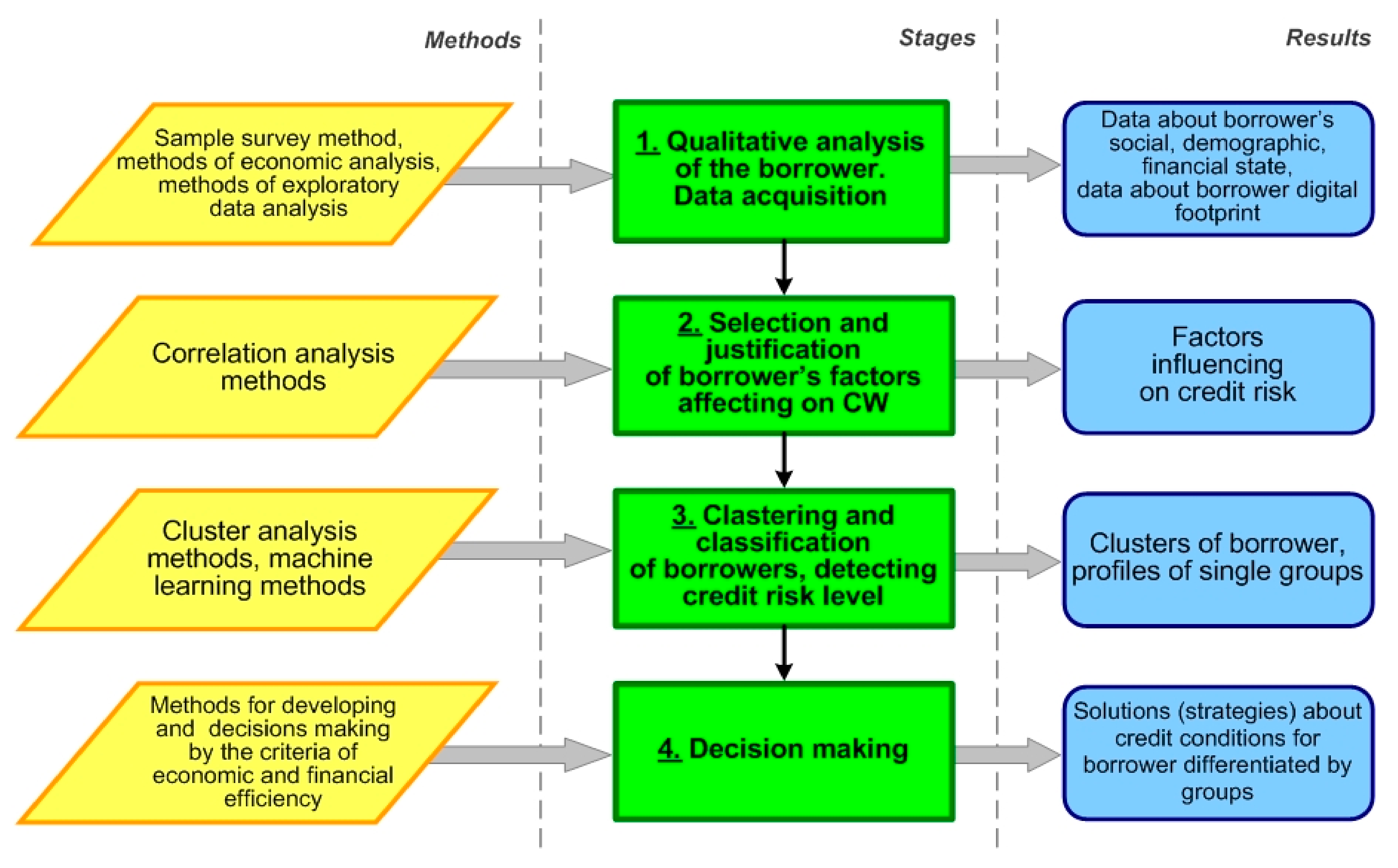
3. Methodology

We propose a methodological approach in the form of information technology based on step-by-step information processing and modeling, reflecting anthropometric and social indicators, financial indicators, and digital footprint data about borrowers. The conceptual diagram of the technology is shown in Figure 1.
Stage 1. Qualitative analysis of borrowers and data acquisition. Analysis of the financial condition of the borrower, the assessment of their atropometric characteristics, and the data of the digital footprint of the borrower is carried out. The result of this stage is collected data about three groups of indicators: anthropometric, financial, and digital footprint data.
Stage 2. Selection and substantiation of factors affecting the borrower’s CW. In this stage, exploratory preliminary data analysis is carried out, and assessment of the influence of factors (anthropometric, financial, and digital footprint) on the borrower’s riskiness is fulfilled on the basis of correlation analysis.
Stage 3. Grouping borrowers with similar profiles into homogeneous clusters. Borrower clustering is carried out from the point of view of the similarity of their anthropometric financial indicator values and indicators about their digital footprints. This stage results in typical risk profiles of borrowers belonging to a qualitatively homogeneous group. In the same stage, the classification of the new borrower is also made, and the borrower group and its riskiness are determined.
Stage 4. Development management decisions about lending conditions. The loan rate and maximum possible loan are formed for each homogeneous borrower’s group and projected onto a specific borrower.
The proposed analysis and modeling technology was tested on data from a large bank of the RF. Data analysis and modeling was investigated using the Statistica 10.0 software package.

Qualitative Analysis of Borrowers and Initial Data Description

The studied indicators, variables, and their values are presented in Table 1.
The initial information about borrowers required for analysis was acquired from different sources and divided into three groups:
  • Anthropometric and social information: gender, age, educational level, profession, marital status, and children;
  • Financial information: regular income, income value, overdue debt, the borrower’s riskiness, and the desired loan value;
  • Digital footprint data obtained from social networks and search engines. Analysis of social media will make it possible to evaluate the borrower’s digital avatar.
The transformation of the qualitative indicators’ values into quantitative ones used binary coding (0 and 1), while the quantitative value increased as its qualitative characteristics intensified.

4. Empirical Results and Analysis

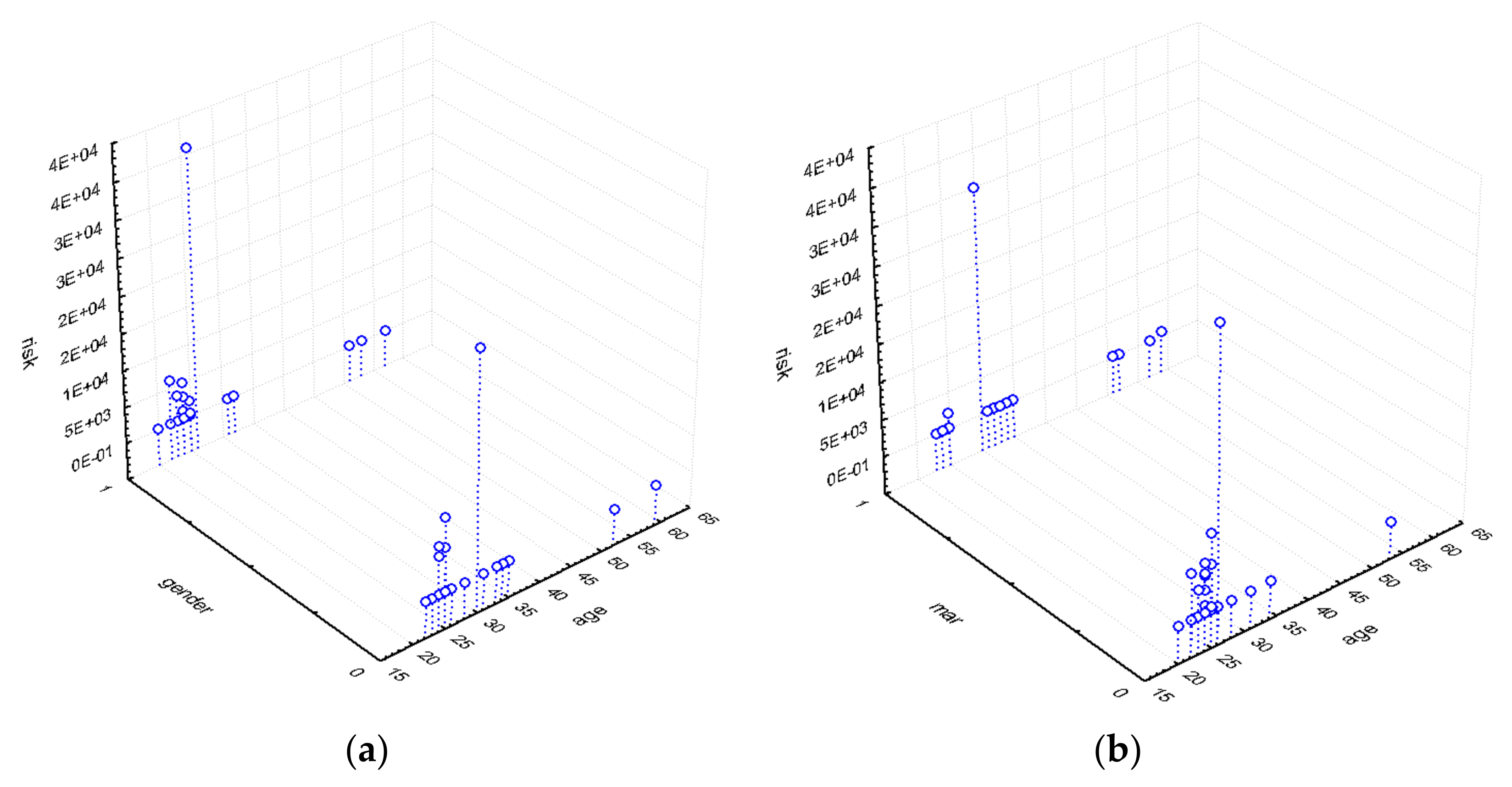
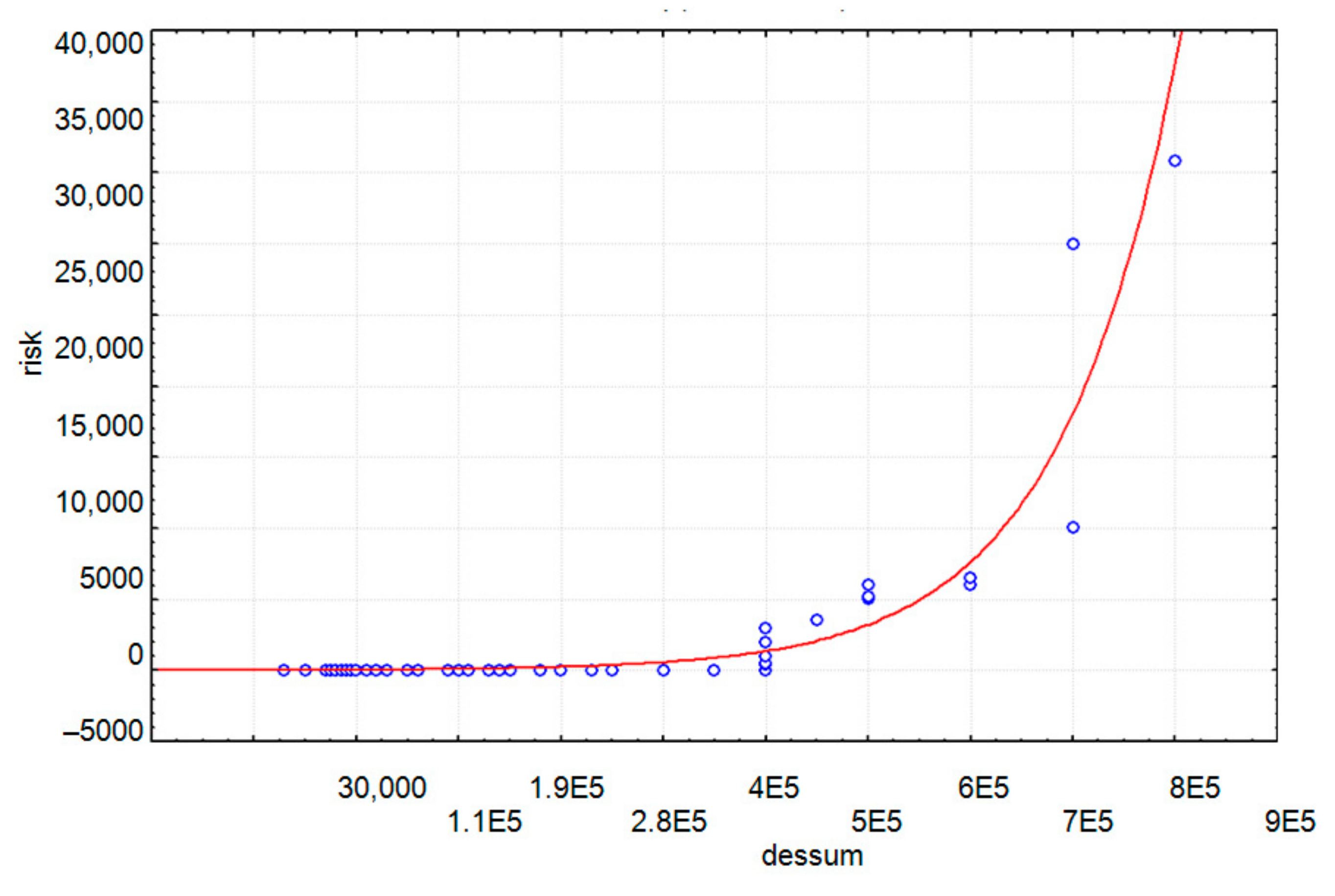
4.1. Selection Factors Affecting the Borrower’s Creditworthiness: Exploratory Data Analysis

For empirical analysis, we used the actual data about borrowers of a large bank of the RF. We tested the proposed technology on data about new borrowers applying for credit. The learning sample was about 100 borrowers and included all the variables indicated in Table 1. We searched for additional information about the borrowers’ digital footprints by ourselves using API tools.
Exploratory data analysis about qualitative factors and their expected impact on the borrowers’ overdue debt (risk) was carried with scope diagrams (Figure 2).
Analysis of the statistical characteristics of risk values depending on the gender (Figure 2a) revealed that men had greater risks than women. The average risk value for men was about 1572 monetary units, and for women it was only 900. However, the figure also shows that the risk variation for men was also higher, while the values of overdue debt among women were almost two times higher, which generally provided approximately the same summary value of overdue debt among men and women.
An analysis of the dependence “risk-bad habits” showed that the total risk of borrowers who did not have bad habits was almost 63% lower and about 44,400 monetary units compared with those of borrowers who had identified bad habits (70,500 monetary units), although the distribution centers and risk variability were not statistically different (Figure 2b). Single borrowers had almost 110% higher risks. Thus, the aggregate risk for single borrowers was 82,400 monetary units, and for married borrowers, it was about 32,500 monetary units. The education level did not affect the borrower risk and was approximately the same for individuals with higher education and for others (about 57,500 monetary units). At the same time, the risk variability for more educated men was much lower. This means that more educated borrowers had greater financial discipline and lower risk for each individual on average over the sample.
The three-dimensional scatterplot (Figure 3) shows that risk was mainly inherent for young borrowers under 35 years of age. Older borrowers posed lower risks, which can be explained by higher financial responsibility and discipline. The data distribution by the variables of “age”, “mar”, and “risk” shows that young unmarried borrowers had high risk. The dependence of the risk value on the loan value is shown in Figure 4, which demonstates that higher risk was inherent for significant values of loans, but in total, loans with low values prevailed.
Descriptive statistics of the risk indicator (Table 2) characterized a significant heterogeneity of the studied data; therefore, to identify dependencies and patterns in the data, it was required to use a classification method (i.e., to divide the initial data into qualitatively homogeneous groups).
To identify paired relationships between the factors and overdue debt (risk), we conducted a correlation analysis. The surveyed indicators were measured on different scales; “risk”, “age”, and “children” had a continuous metric scale, “education level” had an ordinal (i.e., rank) scale, and the other indicators had a nominal (binary) scale. Therefore, analysis of the interrelationships of the investigated factors in order to identify their significant impact on the modeled indicator—the borrower’s risk—should be carried out using different statistical tests. Thus, to measure the relationship between “risk”, “age”, and “children”, we used the Pearson correlation coefficient to assess the effect of “education” on “risk”, Spearman’s rank correlation coefficient, and the impact of categorical variables on “risk” through multivariate variance analysis.
Estimates for the Pearson coefficient (Table 3) for peers classified as “age”-“risk”, “aminc”-“risk”, and “dessum”-“risk” demonstrate that these factors separately did not have a statistically significant effect on the risk value (calculated value of t, where the Student’s criterion is less than tabular at a significance level of 0.05). Calculation of Spearman’s correlation to assess the impact of non-quantitative variables on the risk level revealed a correlation between the borrower’s area of interest and their reliability, as well as a passion for a particular genre of music and reliability. At the same time, the indicator “genre of music” was closely related to a number of factors: the level of education, the sphere of employment, the amount of required credit, the sphere of interests of the borrower, the negative scheme of the environment, and the frequency of visits to sites on the topic of fraud and “gambling”, while the indicator “sphere of interest” had statistically significant association with the indicators of “gender”, “educational level”, “marital status”, “children”, “bad habits”, “bad environment”, “ideal_fam”, as well as “fraud” and “gambling”.
To exclude false correlations, a matrix of partial correlations was built (Table 4), which shows that the variables “ints”, “mus”, and “gambling” significantly affected the borrower’s risk (statistically significant dependencies are marked in red in the figure). In addition, close partial correlations were observed between the factors “dessum” and “gender”, “gambling” and “gender”, “bad_hab” and “gender”, and “mar” and “ideal_fam”, and this was also observed between the pair of factors “gambling” and “ints”. This was due to the presence of bad habits depending on the gender of the borrower, as married borrowers usually have stable relationships in the family, and the frequency of entries on gambling sites is often associated with the presence of unwanted borrower habits.

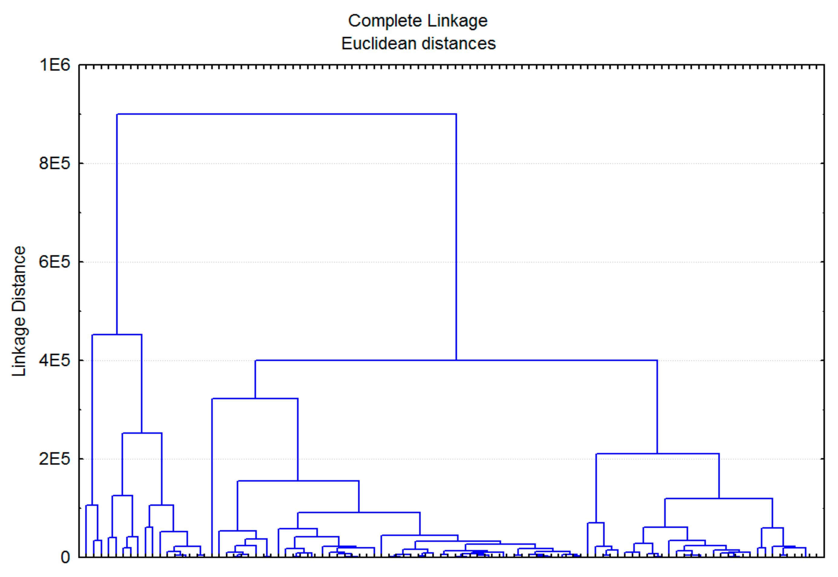
4.2. Model for Borrower Clustering

Here, we use an array of data about qualitative and quantitative indicators obtained at the first technology stage. Those indicators reflect the financial characteristics of borrowers, namely the anthropometric and social characteristics and digital footprint data. In order to smooth out the identified data heterogeneities as well as to order the complex interactions of the factors, we used the procedure of dividing the data into homogeneous groups. These allowed for studying the data and identify patterns in the obtained homogeneous groups in more detail. It was possible that in different groups there would be factors that determined a growth or decline in productivity. Therefore, analysis, modeling, and prediction of the borrowers’ CW over different groups would be carried out on the basis of different models.
Clustering was executed in two stages: qualitative analysis using hierarchical methods and analysis using the k-means method [32,47]. Exploratory analysis to find out the possible number of groups was conducted by the hierarchical classification method. It had different measures of similarity and different objects in the groups: the Euclidean distance, Manhattan distance, and Chebyshev distance to assess the degree of the objects’ proximity within groups and to measure the distances between clusters in a single, complete connection. By changing the distance measurement, we qualitatively assessed the number of clusters.
Analysis of various partitions of the sample by the hierarchical classification method showed that it had from three to five clusters (Figure 5). For a more grounded object grouping, we used cluster methods on the basis of quantitative criteria for the partition. For that, we used the k-means method.
The k-means algorithm is applicable to clustering only numeric data [47]. If there are categorical (qualitative) variables in the initial data, modifications of this algorithm are used, such as the k-modes and k-prototypes algorithm [65,67]. They differ in that they use other measures of the objects’ proximity: the percentage of unconformity and the Euclid–Hamming mixed distance. In this case, the coding procedure was carried out first; that is, the conversion of the values of qualitative characteristics into quantitative ones was performed (see Table 1). In this investigation the mixed Euclidean–Hamming distance was used, and the centroid method was used as a function reflecting the optimality criterion of the partition and expressing the levels of desirability of various alternative partitions. Table 5 shows the results of the clustering, which contains four clusters (k = 4).
The distribution of borrowers in the clusters obtained by the factor levels helped to analyze in more detail the CW level and reveal the distinctive features of borrowers belonging to different groups (Table 6 and Table 7). This made it possible to design borrowers’ profiles for each cluster in order to further decision making. Descriptive statistics of quantitative indicators (Table 6) characterized the significant homogeneity of the resulting borrowers’ clusters.
Categorized histograms in each borrower cluster are shown in Figure 6.
Thus, at this stage, we obtained information about the number of clusters and detailed characteristics of the borrowers in each cluster. The first cluster was the most numerous one. It consisted of married women who were 29 years old with higher education who had jobs with a regular income of an average of RUB 31,531.2, which is consistent with reality. Borrowers in this cluster had no bad habits, with admisable interests in music and films. On average, the desired loan value was RUB 248,125, and the average overdue debt value was RUB 937.5. Their profiles on the internet corresponded to reality. They demonstrated themselves as ideal family men and were not interested in topics like fraud, gambling, or drugs. This cluster was the least risky of all clusters and was characterized by the absence of credit risk.
The second cluster was dominated by single women who were 24 years old with higher education, who had jobs with a regular income of an average of RUB 25,137.93, corresponding to reality, and having no bad habits, with good interests in music and films. On average, the desired loan value was RUB 178,448.3, and the average overdue debt was RUB 172.41. They showed themselves to be imperfect family people, as their profiles on the internet corresponded to reality and they were not interested in topics like fraud, gambling, or drugs. The second cluster had a low level of risk.
In the third cluster, borrowers were mostly single men of 23 years old with secondary specialized education and who had jobs with a regular income of an average value of RUB 38,941.2. On average, the desired loan value was RUB 165,300, and the average overdue debt was RUB 3735.29. They had bad habits, but with a good environment and good interests in music and films. Their profiles and incomes corresponded to reality, and they showed themselves to be imperfect family men. They were not interested in topics like fraud, gambling, or drugs. This cluster was the riskiest, with a high level of credit risk.
The fourth cluster was dominated by unmarried men who were 27 years of age with higher education and who had jobs with a regular income of RUB 38,500.1 on average. On average, the desired loan value was RUB 340,681.8, and the average overdue debt was RUB 159.09. The borrowers in this cluster had bad habits and poor surroundings but with good interests in music and films. Their incomes and profiles were in line with reality. They demonstrated themselves as imperfect family men who were not interested in topics like fraud, gambling, or drugs. This cluster had an average risk value. The final distribution of clusters by levels of credit risk is shown in Table 7.
Based on the identified borrower’s risk (high, medium, low risk, or no risk), in accordance with the instructions of the national bank, credit risk premiums can be calculated by taking into account the bank’s capital adequacy [11]. Considering that the bank’s interest rate on a loan is determined based on the borrowed resource for the bank, the risk premium, the bank’s expenses for obtaining a loan, the bank’s profit, and the risk premium possibly reaching up to 50–70% for the interest rate, its reasonable calculation is significant.

4.3. Model for Borrower Classification

Having received four homogeneous classes of borrowers, we constructed their profiles (a set of characteristics that uniquely distinguished borrowers in different clusters from each other) for further substantiated design of adequate credit risk management strategies. The challenge was to determine the group and, accordingly, the profile that the new borrower had. To solve this problem, we needed to make a classification model. This model should detect the cluster to which that borrower belongs. We selected methods and determined their comparative efficiencies for the classification. The classification model must be robust for input data noise and give highly accurate results.
We considered the following types of classifiers: metric, linear, and boosting. Metric classifiers are easy to use, as they use the analysis of the objects’ similarities in the sample with training methods, but they are not flexible; they are unstable to data noise and outliers in the initial data. Linear classifiers are flexible algorithms, but they are limited in that they assign objects to one of two classes; that is, they are used for binary classification. For the problem to be solved, this classifier was not suitable. The third type of classifiers, boosting, allows for combining weak classifiers into one strong one, and on the basis of combination, they can eliminate the shortcomings of each algorithm.
The use of a metric classifier based on the KNN algorithm and boosting based on the SGB algorithm for the challenge of new borrower classification showed the following accuracy results. The classification quality assessment was estimated by the number of correct predictions of the cluster to which the borrower belonged in the test sample (75% of borrower data were used as a training sample, and 25% were used as a test sample). Thus, in the KNN-based model, 83.4% correct assignments of borrowers to clusters was obtained, and in the SGB-based model, 94.1% correct predictions was obtained.
The efficiency of the classification model was determined by the proportion of correct predictions. As a metric indicator of the classification quality, the “accuracy” indicator was used for measuring the model’s general error. This was determined by comparing the model results with the true value of the credit risk. It was formed as the ratio of correctly classified objects in the sample (dataset) (Figure 7). The learning curve shows that the increase of the dataset had no impact on the trained model.
Thus, it was shown that for the SGB model under a set of categorical (qualitative) predictors, all variables about the digital footprints of the borrowers predicted the borrowers’ classes with high accuracy (i.e., the borrowers’ risk profiles). The KNN model was most suitable for prediction under many quantitative predictors.
Boosting is one of the most powerful recognition algorithms. This is for the adaptive technique of composition construction [70,71]. Taking into account the features of the problem being solved, it was possible to select a set of basic algorithms and a loss function [72,73], which was to focus on the processed data features. We proposed using stochastic gradient boosting (SGB), which consists of algorithms that represent boosting as a gradient descent process. The algorithm is based on the sequential refinement of a function, which is a linear combination of basic classifiers used to minimize the loss function. Next, we consider the classification model based on the boosting algorithm in more detail.

Statement of the Classification Problem

There are many borrowers X and many non-overlapping credit risk classes Y to which borrowers belong. There is an objective function y * : X Y whose values y i = y * x i are known only for a finite subset of objects x 1 , , x l X . The set X l = x i , y i i = 1 l forms a training sample of borrowers with numbers of the risk classes.
In general, the training is to restore the dependence y * from the sample X l that is to construct a decision function (algorithm) a : X Y , which approximates the objective function y * x not only for the objects of the training sample, but also for the entire set X. In the classification problem being solved, there are M disjointed classes y 1 , , y M Y . In this case, the entire set of objects X is divided into classes H y = x X : y * x = y , and the algorithm a x gives an answer to the question of which class the borrower x belongs to.
When solving classification problems, it often occurs that none of the algorithms used provide the required prediction accuracy. One of the alternative solutions can be the construction of compositions of these algorithms to compensate for these shortcomings. A composition of K algorithms a k x = C b k x , k = 1 , , K is a superposition of algorithmic operators b k : X R , a correcting operation F : R k R , and a decision rule C : R Y : a x = C F b 1 x , b K x , x X . The algorithmic composition will have the following form:
a x = C F b 1 x , b K x = arg max y Y k = 1 K a k b k x , x X .
That is to say, the classification algorithm a k : X b k R C Y has the following structure and sequence of steps. First, b x calculates some estimate of the borrower’s getting into a particular class. Then, using the decision rule, the algorithm translates them into the final result: the class number. With the help of the space of estimates R , the set of admissible corrective operations is expanded, since when determining F , how a mapping Y t Y arises is the problem of choosing an acceptable F as an aggregating function or a meta-algorithm. When combining the responses of algorithmic operators, the operation uses estimates of the borrowers belonging to classes that are more accurate. We will use linear combinations (weighted voting) and adjust our coefficient for each basic algorithm.
The quality function of the algorithm in Equation (1) is defined as the number of errors made in the training sample:
Q K = j = 1 l arg max y Y k = 1 K a k b k ( x j ) y j
The task is to minimize the function in Equation (2). To simplify this, we introduce a heuristic. The threshold loss function of the quality functional is replaced by a continuously differentiable upper bound L M . This estimate is one of the variable parameters:
Q K Q K = i = 1 l L k = 1 K a k b k x i , y i
In order to minimize the function in Equation (2), we introduce one more heuristic. When adding the k-th term, only the k-th basic algorithm and its coefficient are optimized, and all previously introduced terms remain fixed. With the help of this technique, a set of basic algorithms is optimized; that is, when training the next algorithm, the weight of the objects for which a classification error was made increases. Thus, it is possible to take into account the errors of the previous basic algorithms. Taking into account the rate of training η (gradient step), we have
Q η , b ; X l = i = 1 l L k = 1 K 1 a k b k x i + η b x i , y i min η , b .
Additionally, we introduce the following notation:
f K 1 = f K 1 , i i = 1 l = k = 1 K 1 a k b k x i i = 1 l :   the   current   approximation .
f K = f K , i i = 1 l = k = 1 K 1 a k b k x i + η b x i i = 1 l :   the   next   approximation .
To minimize the function Q f , we use the gradient method, initially not paying attention to the fact that f K has involuntary coordinates. Having obtained the result, we will further approximate it using a and b. Let us use the initial approximation
f 0 : = 0 , f K , i : = f K 1 , i η g i , i = 1 , , l ;
where g i = L f K 1 , i , y i is the components of the vector gradient and η is the gradient step (learning rate).
Having determined the vector gradient, we approximate it with the basic algorithm b k so that b k x i i = 1 l , which approximates the vector g i i = 1 l :
b K : = arg max b i = 1 l b x i + g i 2
The step in Equation (8) reflects the main idea of boosting: the sequential construction of the compositions of the algorithms, in which each subsequent algorithm strives to compensate for the shortcomings of the compositions of all previous ones. The function is minimized using the gradient step, and as a result, a new basic algorithm is obtained.
The formal Algorithm (Algorithm 1) of the method is represented as follows:
Algorithm 1 Search for basic algorithms and their weights
 Input: training sample X l ; number of iterations K; learning step η .
 Output: basic algorithms and their weights a k b k , k = 1 , , K .
  • Initialize f i : = 0 , i = 1 , , l ;
  • For all of them, k = 1 , , K :
  • Find a basic algorithm that approximates the antigradient
b K : = arg min b i = 1 l b x i + L f i , y i 2 ;
4.
Solve the one-dimensional minimization problem
a k : = arg min a > 0 i = 1 l L f i + η b k x i , y i 2 ;
5.
Update the composition values over the sample.
Objects from the training sample were randomly selected, and the loss function was given as a logarithmic function. It should be noted that the main tools for tuning the SGB algorithm were the number of basic algorithms as well as the step of the gradient method.
The homogeneous borrowers’ groups with substantively different profiles designed at this technology stage provided a basis for the development of differentiated management decisions (strategies) for operational managing of the bank’s credit risks. Such strategies were developed separately for each of the four homogeneous clusters. Management decisions were aimed at the monitoring and prevention of individual loan defaults.

5. Discussion of Results

5.1. Comparative Analysis of Different Borrower Classification Models

To assess the effectiveness of the proposed classification model, we compared different classification algorithms. We tested a regression model (R-model) based on the logit transformation method [32,34] and the proposed classification model based on machine learning methods (ML-model). Since logit regression is used to solve binary classification problems, we divided the entire sample of borrowers into two groups, reliable and risky, referring borrowers without risk (reliable borrower) to the group numbered “0” and risky borrowers to group “1”. We compared the models by their predictive performance and executed a binary classification. Since the sample of borrowers was not balanced and there were significantly fewer overdue borrowers, class “1” was predominant. Class “1” in this case was more important and of greater interest from the point of view of prediction, since the incorrect classification of class “1” was more expensive for the bank than the incorrect classification of class “0”. On the other hand, the correct identification of a reliable borrower will allow the bank to save the cost and effort of manually reviewing the borrower’s data and conducting a more comprehensive analysis.
Receiver operator characteristic (ROC) curves are commonly used to present results for binary decision problems in machine learning [74,75]. However, when dealing with highly skewed datasets, precision-recall (PR) curves give a more informative picture of an algorithm’s performance.
The decision determined by the classifier was represented using the confusion matrix. There were four cells highlighted in the matrix. True positives (TP) were examples correctly labeled as positives. False positives (FP) were examples incorrectly flagged as positives. Examples that were correctly labeled as negative were true negatives (TNs), and examples that were mistakenly labeled as negative were false negatives (FNs). The confusion matrix for the frequency of correct predictive estimates based on the regression model is shown in Table 8. The confusion matrix for the frequency of correct predictive estimates based on the machine learning model is shown in Table 9.
When plotting the ROC curve, the abscissa represents the false positive rate (FPR) and the ordinate represents the true positive rate (TPR). The FPR indicator shows the proportion of negative examples that were mistakenly classified as positive. The TPR indicator shows the proportion of positive examples that were correctly classified. When plotting the PR curve, the abscissa represents the recall (which was the same as the TPR), and the ordinate shows the precision (characterized the share of the examples that were classified as positive which were really positive). The goal in the ROC space is to be in the upper-left-hand corner, and in the PR space, the goal is to be in the upper-right-hand corner.
The area under the ROC curve (AUC-ROC) is a measure of the quality of the classification model as a whole. The area under the curve is defined as the sum of the trapezoidal areas between the ROC points. The area under the PR curve (AUC-PR) was calculated by the same method. The differencies between comparing the models in ROC and PR space for the sample size n = 100 are given in Figure 8.
For dataset n = 100, the AUC-ROC for the ML-model was 0.61, and the AUC-ROC for the R-model was 0.52, so the ML-model had the higher predictive power to identify risky borrowers. The AUC-PR for the ML-model was 0.27, and the AUC-PR for the R-model was 0.42; that is, in general, the R-model was more accurate for the small dataset. Thus, from the point of view of the predictive power of the borrower’s risk, the model which more accurately identified risky borrowers as really risky is preferred more compared with the others, although it had a lower accuracy in general for the small dataset.
A series of simulation experiments was conducted to determine the relationship between the accuracy of the machine learning model and the borrower’s sample size. It is shown that with an increase in the borrower’s sample size, the prediction accuracy of a risky borrower increased (Figure 9).
Thus, when predicting rare events, the machine learning model gave more correct results in comparison with the regression models. To predict risky borrowers, it was preferable to use a machine learning model.

5.2. Comparative Analysis of the Proposed Methodology and Models with the Traditional Credit Scoring Model

The organization of management decisions to minimize the bank’s credit risks due to inaccurate loan payments by individuals is based on loan portfolio diversification. Diversification of the bank’s loan portfolio is a method for minimizing credit risk based on the individual lending conditions for each group of borrowers, including loan terms, the types of loan collateral, and the maximum of loan value [69]. Diversification is carried out with various criteria, including the sectoral segment, geographic location, capital size, ownership, risk/return ratio, and obligations.
Comparative analysis of the effectiveness of the proposed methodological approach and the traditional approach for individual CW assessment yielded the following results. CW assessment by the existing (basic) methodology, which consists of a three-stage procedure (initial verification of borrowers for compliance with loan conditions, implementation of credit scoring according to basic indicators, and final assessment of the borrower’s CW), is demonstated in Table 10, Table 11 and Table 12.
CW assessment by the existing creditworthiness methodology gave the following results: all borrowers were reliable and could be issued a loan. For comparison, the same borrowers were assessed using the proposed methodology. The results of this assessment are shown in Table 13. A comparison of the borrowers’ reliability in terms of their CW is given in Table 14.
The aggregate risk associated with an incorrect assessment of the CW, riskiness, and reliability of borrowers was about RUB 275,000 for the presented sample, and for the entire analyzed borrowers set, this value would be more than RUB 5 million. Taking into account that the implementation of the proposed methodology with software and training of credit department employees would cost about RUB 1 million, the net profit per year for the bank would be more than RUB 4 million.

6. Conclusions

The aim of this research to develop a methodology for potential borrower CW assessment from the perspective of his or her risk profile, to design new models for clustering and for classification in the framework of the supposed methodology using social, antropometric, and financial indicators, characterizing not just the borrower but also the additional indicators of his or her digital footprint, was fully achieved. The suggested methodology as an adequate tool for borrower CW assessment ensured the reduction of credit risks for financial organizations and increased the efficiency of their functioning. A model for borrower clustering based on the method of hierarchical clustering and the k-means method was designed, which grouped actual borrowers having similar CW scores and similar values of credit risk into homogeneous clusters. A model for borrower classification based on the stochastic gradient boosting (SGB) method was constructed which reliably determined the number of cluster and therefore the risk level for a new borrower.
These new results were obtained over the course of the investigation:
  • The new factors for a comprehensive assessment of the borrower’s risk profile were compiled as well as economically and financially substantiated. The data about borrowers, collected on the basis of their digital footprints, reflected more complete and adequate borrower digital profiles and should be included in the methodology that, in turn, helps a financial organization to design individual credit trajectories for each borrower and to improve the issued loans’ quality.
  • A new methodological approach for borrower CW assessment was proposed, which was designed to reduce credit risks and increase a bank’s financial stability.
  • Models for clustering and classification were suggested which, by being a part of the methodology, gave more reliable results about borrower risk profiles and were the basis for making decisions about loan conditions for new borrowers. Application of these models increased the efficiency of financial decisions.
The reliability and validity of the obtained results were determined by the adequacy of the selected mathematical tools for the research object and confirmed with real data. Economic efficiency of the improved methodology for borrower CW assessment was confirmed. The introduction of the obtained results into practice would contribute to the sustainable development of financial organizations.

Funding

This research received no external funding.

Institutional Review Board Statement

Not applicable.

Informed Consent Statement

Not applicable.

Data Availability Statement

Not applicable.

Conflicts of Interest

The author declares no conflict of interest.

References

  1. Principles for the Management of Credit Risk. Basel Committee on Banking Supervision. 2000. Available online: https://www.bis.org/publ/bcbs75.pdf (accessed on 20 February 2021).
  2. Basel Committee on Banking Supervision. International Convergence of Capital Measurement and Capital Standards. A Revised Framework; Consultative Document; Bank for International Settlements: Basel, Switzerland, 2004; Available online: https://www.bis.org/publ/bcbs128.pdf (accessed on 20 February 2021).
  3. Basel Committee on Banking Supervision. International Regulatory Framework for Banks; Consultative Document; Bank for International Settlements: Basel, Switzerland, 2010; Available online: https://www.bis.org/bcbs/basel3.htm (accessed on 20 February 2021).
  4. Pestova, A.; Mamonov, M. Macroeconomic and Bank-Specific Determinants of Credit Risk: Evidence from Russia; EERC Working Paper Series 13/10E; Economics Education and Research Consortium: Kyiv, Ukraine, 2013. [Google Scholar]
  5. Chernikova, L.I.; Faizova, G.R.; Egorova, E.N.; Kozhevnikova, N.V. Functioning and Development of Retail Banking in Russia. Mediterr. J. Soc. Sci. 2015, 6, 274–284. [Google Scholar] [CrossRef] [Green Version]
  6. Kjosevski, J.; Petkovski, M. Non-performing loans in Baltic States: Determinants and macroeconomic effects. Balt. J. Econ. 2017, 1, 25–44. [Google Scholar] [CrossRef] [Green Version]
  7. Fainstein, G.; Novikov, I. The comparative analysis of credit risk determinants in the banking sector of the Baltic States. Rev. Econ. Financ. 2011, 1, 20–45. [Google Scholar]
  8. Shai, S.-S.; Shai, B.-D. Understanding Machine Learning: From Theory to Algorithms; Cambridge University Press: Cambridge, UK, 2014; p. 294. [Google Scholar]
  9. Leo, M.; Sharma, S.; Maddulety, K. Machine Learning in Banking Risk Management: A Literature Review. Risk 2018, 7, 29. [Google Scholar] [CrossRef] [Green Version]
  10. Saqib, A.; Dowling, M.M. AI and Machine Learning for Risk Management. Available online: https://library.oapen.org/bitstream/handle/20.500.12657/23126/1007030.pdf?sequence=1#page=54 (accessed on 20 February 2021).
  11. Instruction of the Bank of Russia. On Mandatory Ratios and Surcharges to Capital Adequacy Ratios for Banks with a Universal License; Bank of Russia: Moscow, Russia, 2019; Available online: https://rudata.info/files/rudata/add-in/documents/199-i.pdf (accessed on 20 February 2021).
  12. Provision on the Procedure for the Formation by Credit Organizations of Reserves for Possible Losses on Loans, Loan Debt and Equivalent Debt. Available online: https://base.garant.ru/71721612/ (accessed on 20 February 2021).
  13. Lunyakova, N.A.; Lavrushin, O.I.; Lunyakov, O.V. Clustering the regions of the Russian Federation by the level of deposit risk. Econ. Reg. 2018, 3, 1046–1060. [Google Scholar]
  14. Lavrushin, O.I. The Development of the Banking Sector and Its Infrastructure in the Russian Economy; KNORUS: Moscow, Russia, 2017; p. 176. [Google Scholar]
  15. Tobin, P.; Brown, A. Estimation of Liquidity Risk in Banking. ANZIAM J. 2004, 45, 519–533. [Google Scholar] [CrossRef] [Green Version]
  16. Allan, J.; Boot, P.; Verrall, R.; Walsh, D. The Management of Risks in Banking. Br. Actuar. J. 1998, 4, 707–802. [Google Scholar] [CrossRef]
  17. Kuznetsov, I.V.; Zhevaga, A.A. Stress testing of credit risk in a commercial bank on the basis of macroeconomic indicators. Financ. Risk Manag. 2018, 1, 2–11. [Google Scholar]
  18. Shamrina, S.Y.; Lomakina, A.N. Scenario analysis of stress testing in assessing the main types of risks of a credit institution. Financ. Credit 2018, 24, 1736–1750. [Google Scholar] [CrossRef]
  19. Kurennoy, D.S. Algorithm for solving the problem of reverse stress testing the bank’s loan portfolio based on system-dynamic models of borrowers. Int. J. Open Inf. Technol. 2018, 10, 9–21. [Google Scholar]
  20. Principles for Sound Stress Testing Practices and Supervision. Basel Committee on Banking Supervision. 2009. Available online: https://www.bis.org/publ/bcbs155.pdf (accessed on 25 February 2021).
  21. Kazansky, A.V. Functioning of the Internal Rating System of a Commercial Bank. Probl. Mod. Econ. 2016, 4, 127–131. [Google Scholar]
  22. Dedova, M.S. Comparing the bootstrap methods of time series for the purpose of backtesting banking risk assessment models. Econ. J. HSE 2018, 22, 84–109. [Google Scholar] [CrossRef]
  23. Rashevskikh, M.A. Methods of credit portfolio management in Russia. Econ. Sociol. 2017, 1, 32–34. [Google Scholar]
  24. Ruiz, I. XVA: Desks—A New Era for Risk Management; Palgrave Macmillan UK: London, UK, 2015; p. 433. [Google Scholar]
  25. Basel Committee on Banking Supervision. Sound Practices for Backtesting Counterparty Credit Risk Models. 2010. Available online: https://www.bis.org/publ/bcbs185.pdf (accessed on 25 February 2021).
  26. Bronshtein, E.M.; Shaposhnikova, A.G. Portfolio optimization based on complex index risk measures. Audit Financ. Anal. 2010, 5, 220–224. [Google Scholar]
  27. Orlova, E.V. The AI Model for Identification the Impact of Irrational Factors on the Investor’s Risk Propensity. In Proceedings of the 30th International Business Information Management Association Conference (IBIMA), Vision 2020: Sustainable Economic Development, Innovation Management, and Global Growth, Madrid, Spain, 8–9 November 2017; pp. 713–721. [Google Scholar]
  28. Saaty, T. Decision Making with Dependencies and Feedback, Analytic Networks; LKT Publishing House: Moscow, Russia, 2008; p. 360. [Google Scholar]
  29. Rockafellar, R.T.; Uryasev, S. Conditional Value-at-Risk for General Loss Distribution. J. Bank. Financ. 2002, 26, 1443–1471. [Google Scholar] [CrossRef]
  30. Rockafellar, R.T.; Uryasev, S. Optimization of Conditional Value-At-Risk. J. Risk 2003, 2, 21–41. [Google Scholar] [CrossRef] [Green Version]
  31. Rachev, S.T.; Menn, C.; Fabozzi, F.J. Fat-Tailed and Skewed Asset Return Distributions. Implications for Risk Management, Portfolio Selection and Option Pricing; John Wiley & Sons: Hoboken, NJ, USA, 2005; p. 369. [Google Scholar]
  32. Orlova, E.V. Economic Efficiency of the Mechanism for Credit Risk Management. In Proceedings of the Workshop on Computer Modelling in Decision Making (CMDM 2017), Saratov, Russia, 14–15 November 2019; pp. 139–150. [Google Scholar]
  33. Niu, B.; Ren, J.; Li, X. Credit Scoring Using Machine Learning by Combing Social Network Information: Evidence from Peer-to-Peer Lending. Information 2019, 10, 397. [Google Scholar] [CrossRef] [Green Version]
  34. Orlando, G.; Pelosi, R. Non-Performing Loans for Italian Companies: When Time Matters. An Empirical Research on Estimating Probability to Default and Loss Given Default. Int. J. Financ. Stud. 2020, 8, 68. [Google Scholar] [CrossRef]
  35. Bankova, V.K. Scoring Models to Assess the Creditworthiness of Borrowers in Russia. Izv. Acad. Man. 2011, 4, 14–16. [Google Scholar]
  36. Glinkina, E.V. Credit Scoring as a Tool for Effective Credit Assessment. Financ. Credit. 2011, 16, 43–47. [Google Scholar]
  37. Lebedev, E.A. Synthesis of Scoring Models Method of Systemic-Cognitive Analysis. Polythematic Netw. Electron. Sci. J. Kuban State Agrar. Univ. 2007, 29, 17–30. [Google Scholar]
  38. Makarenko, T.M. The Combination of Scenario Forecasting Procedures with the Dynamic Ranking of Experts when Assessing the Credit Risk of the Borrower—Physical Persons in the Bank. Bull. Leningr. State Univ. A. S. Pushkin. 2012, 3, 56–63. [Google Scholar]
  39. Crone, S.F.; Finlay, S. Instance Sampling in Credit Scoring: An Empirical Study of Sample Size and Balancing. Int. J. Forecast. 2012, 28, 224–238. [Google Scholar] [CrossRef]
  40. Crook, J.N.; Edelman, D.B.; Thomas, L.C. Recent Developments in Consumer credit Risk Assessment. Eur. J. Oper. Res. 2007, 3, 1447–1465. [Google Scholar] [CrossRef]
  41. Mircea, G.; Pirtea, M.; Neamţu, M.; Băzăvan, S. Discriminant Analysis in a Credit Scoring Model. Recent Adv. Appl. Biomed. Inform. Comput. Eng. Syst. Appl. 2011, 2, 56–69. [Google Scholar]
  42. Ong, C.; Huang, J.; Tzeng, G. Building Credit Scoring Models Using Genetic Programming. Expert Syst. Appl. 2005, 9, 41–47. [Google Scholar] [CrossRef]
  43. Aebi, V.; Sabato, G.; Schmid, M. Risk management, corporate governance, and bank performance in the financial crisis. J. Bank. Financ. 2012, 12, 3213–3226. [Google Scholar] [CrossRef]
  44. Berger, A.N.; Sedunov, J. Bank liquidity creation and real economic output. J. Bank. Financ. 2017, 81, 3213–3226. [Google Scholar] [CrossRef]
  45. Caporale, G.M.; Cerratot, M.; Zhang, X. Analyzing the Determinants of Insolvency Risk for General Insurance Firms in the UK. J. Bank. Financ. 2017, 84, 107–122. Available online: http://www.sciencedirect.com/science/article/pii/%20S0378426617301711 (accessed on 1 November 2020). [CrossRef]
  46. Basulin, M.A. Analysis Software «Sas Credit Scoring» for the Commercial Bank. Innov. Inf. Technol. 2013, 2, 32–37. [Google Scholar]
  47. Orlova, E.V. Mechanism for Credit Risk Management. In Proceedings of the 30th International Business Information Management Association Conference (IBIMA), Vision 2020: Sustainable Economic Development, Innovation Management, and Global Growth, Madrid, Spain, 8–9 November 2017; pp. 827–837. [Google Scholar]
  48. Mehra, R.; Prescott, E.C. The Equity Premium: A Puzzle. J. Monet. Econ. 1985, 5, 145–161. [Google Scholar] [CrossRef]
  49. Benartzi, S.; Thaler, R. Myopic Loss Aversion and the Equity Premium Puzzle. Q. J. Econ. 1995, 110, 75–92. [Google Scholar] [CrossRef] [Green Version]
  50. Ang, A.; Bekaert, G.; Liu, J. Why Stocks May Disappoint. J. Financ. Econ. 2000, 76, 471–508. [Google Scholar] [CrossRef] [Green Version]
  51. Fielding, D.; Stracca, L. Myopic Loss Aversion, Disappointment Aversion, and Equity Premium Puzzle; Working Paper Series; European Central Bank: Frankfurt, Germany, 2003. [Google Scholar]
  52. Khandani, A.E.; Kim, A.J.; Lo, A.W. Consumer credit risk models via machine learning algorithms. J. Bank. Financ. 2010, 34, 2767–2787. [Google Scholar] [CrossRef] [Green Version]
  53. McKinsey—Analytics in Banking. 2017. Available online: https://www.mckinsey.com/industries/financial-services/%20our-insights/analytics-in-banking-time-to-realize-the-value (accessed on 19 March 2021).
  54. McKinsey’s Global Banking Annual Review. 2020. Available online: https://www.mckinsey.com/industries/financial-services/our-insights/global-banking-annual-review (accessed on 19 March 2021).
  55. Bhatore, S.; Mohan, L.; Reddy, Y.R. Machine learning techniques for credit risk evaluation: A systematic literature review. J. Bank Financ. Technol. 2020, 4, 111–138. [Google Scholar] [CrossRef]
  56. Machine Learning for Asset Management: New Developments and Financial Applications. ISTE Ltd. 2020. Available online: https://onlinelibrary.wiley.com/doi/book/10.1002/9781119751182 (accessed on 20 March 2021).
  57. Bagherpour, A. Predicting Mortgage Loan Default with Machine Learning Methods. 2017. Available online: https://www.semanticscholar.org/paper/Predicting-Mortgage-Loan-Default-with-Machine-Bagherpour/a4e53d7255dd397da78242c4ad41213a404cb51e (accessed on 19 March 2021).
  58. Maheswari, P.; Narayana, C.V. Predictions of Loan Defaulter—A Data Science Perspective. In Proceedings of the 5th International Conference on Computing, Communication and Security (ICCCS), Patna, India, 14–16 October 2020; pp. 1–4. [Google Scholar] [CrossRef]
  59. Sivasree, M.S. Loan Credibility Prediction System Based on Decision Tree Algorithm. Int. J. Eng. Res. Technol. 2015. [Google Scholar] [CrossRef]
  60. Krichene, A. Using a naive Bayesian classifier methodology for loan risk assessment. J. Econ. Financ. Adm. Sci. 2017, 22, 3–24. [Google Scholar] [CrossRef]
  61. Namvar, A.; Siami, M.; Rabhi, F.; Naderpour, M. Credit risk prediction in an imbalanced social lending environment. Int. J. Comput. Intell. Syst. 2018, 11, 925–935. [Google Scholar] [CrossRef] [Green Version]
  62. Sudhamathy, G. Credit Risk Analysis and Prediction Modelling of Bank Loans Using R. Int. J. Eng. Technol. 2016, 8, 1954–1966. [Google Scholar] [CrossRef] [Green Version]
  63. Semiu, A.; Gilal, A. A Boosted Decision Tree Model for Predicting Loan Default in P2P Lending Communities. Int. J. Eng. Adv. Technol. 2019, 9. [Google Scholar] [CrossRef]
  64. Uzair, A.; Ilyas, T.; Asim, S.; Nowshath, B. An Empirical Study on Loan Default Prediction Models. J. Comput. Theor. Nanosci. 2019, 16, 3483–3488. [Google Scholar] [CrossRef]
  65. Orlova, E.V. Model for Operational Optimal Control of Financial Recourses Distribution in a Company. Comput. Res. Modeling 2019, 2, 343–358. [Google Scholar] [CrossRef] [Green Version]
  66. Orlova, E.V. Technology for Control an Efficiency in Production and Economic System. In Proceedings of the 30th International Business Information Management Association Conference (IBIMA). Vision 2020: Sustainable Economic Development, Innovation Management, and Global Growth, Madrid, Spain, 8–9 November 2017; pp. 811–818. [Google Scholar]
  67. Orlova, E.V. Synergetic Approach for the Coordinated Control in Production and Economic System. In Proceedings of the 30th International Business Information Management Association Conference (IBIMA). Vision 2020: Sustainable Economic development, Innovation Management, and Global Growth, Madrid, Spain, 8–9 November 2017; pp. 704–712. [Google Scholar]
  68. Orlova, E.V. Control over Chaotic Price Dynamics in a Price Competition model. Autom. Remote Control 2017, 78, 16–28. [Google Scholar] [CrossRef]
  69. Orlova, E.V. Decision-Making Techniques for Credit Resource Management Using Machine Learning and Optimization. Information 2020, 11, 144. [Google Scholar] [CrossRef] [Green Version]
  70. Friedman, J. Stochastic Gradient Boosting. Comput. Stat. Data Anal. 1999, 38, 367–378. [Google Scholar] [CrossRef]
  71. Friedman, J. Greedy Function Approximation: A Gradient Boosting Machine. Ann. Stat. 2001, 29, 1189–1232. [Google Scholar] [CrossRef]
  72. Mason, L.; Baxter, J.; Barlett, R.; Frean, M. Boosting Algorithm as Gradient Descent. Advances in Neural Information Processing Systems Computational Statistics and Data Analysis; MIT Press: Cambridge, MA, USA, 2000; Volume 12, pp. 512–518. [Google Scholar]
  73. Hastie, T.; Tibshriani, R.; Friedman, J. The Elements of Statistical Learning; Springer: Berlin, Germany, 2014; p. 739. [Google Scholar]
  74. Provost, F.; Fawcett, T.; Kohavi, R. The case against accuracy estimation for comparing induction algorithms. In Proceedings of the 15th International Conference on Machine Learning, Morgan Kaufmann, San Francisco, CA, USA, 24–27 July 1998; pp. 445–453. [Google Scholar]
  75. Davis, J.; Goadrich, M. The Relationship Between Precision-Recall and ROC Curves. In Proceedings of the 23rd International Conference on Machine Learning, ACM, Pittsburgh, PA, USA, 25–29 June 2006. [Google Scholar] [CrossRef] [Green Version]
Figure 1. Conceptual scheme of the technology for individual creditworthiness (CW) assessment.
Mathematics 09 01820 g001
Figure 2. Diagrams about the ranges for factor groups such as gender and risk (a), bad_hab and risk (b), mar and risk (c), and edu and risk (d).
Mathematics 09 01820 g002
Figure 3. 3D scatter plots by factor groups: age, gender, and risk (a) and age, mar, and risk (b).
Mathematics 09 01820 g003
Figure 4. Graph of the dependence of the risk on loan value (“dessum”).
Mathematics 09 01820 g004
Figure 5. Dendrogram of hierarchical clustering.
Mathematics 09 01820 g005
Figure 6. Distribution of borrowers over clusters by levels of categorized variables: gender (a), edu (b), empl (c), mar (d), avinc (e), bad_hab (f), ints (g), bad_env (h), mus (i), mov (j), inc (k), ideal_fam (l), profile (m), fraud (n), and illness (o). Distribution of borrowers over clusters by levels of categorized variables: gambling (p), career (q), and drugs (r).
Mathematics 09 01820 g006aMathematics 09 01820 g006b
Figure 7. Learning curves.
Mathematics 09 01820 g007
Figure 8. The differencies between comparing the models in ROC and PR space (sample size n = 100) for the ML-model in AUC-ROC space (a), ML-model in AUC-PR space (b), R-model in AUC-ROC space (c), and R-model in AUC-PR space (d).
Mathematics 09 01820 g008aMathematics 09 01820 g008b
Figure 9. Comparative characteristics of the ML-models in ROC and PR space for different sample sizes: ML-model in AUC-ROC space where n = 200 (a), ML-model in AUC-PR space where n = 200 (b), ML-model in AUC-ROC space where n = 300 (c), and ML-model in AUC-PROC space where n = 300 (d).
Mathematics 09 01820 g009
Table 1. Investigated indicators, designations, and range of values.
Indicator GroupIndicatorVariableRange of Value or Binary
anthropometric and social indicatorsgendergenderfemale (1), male (0)
ageage18…65
education leveledusecondary, specialized (0),
higher (1)
professionproofany profession (1),
no profession (0)
housewife, student (0)
family statusmarsingle (0), married (1)
childrenchild0, 1, 2, 3, …
finantial indicatorsregular incomeavincyes (1), no (0)
income valueaminc0...1000000
loan valuedessum0...1000000
overdue debt value (risk)risk0...1000000
bad habitsbad_habyes (1), No (0)
interestsintse.g., career, family, philosophy (1), anti-collector, gambling (0)
bad environmentbad_env1 or more (0), 0 (1)
music stylemusclassical, pop, jazz (1),
prison nature, prohibited
in the RF (0)
film genremove.g., comedy, family, drama (1),
prohibited in the RF (0)
confirmed incomeinccompliant (1), differs (0)
ideal family manideal_famyes (1), no (0)
digital footprint databorrower profile assessmentprofilecompliant (1), differs (0)
frequency of entries to the site on the subject of fraudfraud1 or more (0),
less than 1 (1)
frequency of entries to the site on the topic of diseasesillness1 or more (0),
less than 1 (1)
frequency of entries to the site related to gamblinggambling1 or more (0),
less than 1 (1)
frequency of entries to the site on the topic of drug distribution and usedrugs1 or more (0),
less than 1 (1)
frequency of entries to the site on the subject of banned organizations in the RFforbidden1 or more (0),
less than 1 (1)
frequency of entries to the site on the topic of business development and self-developmentcareer1 or more (0),
less than 1 (1)
Table 2. Descriptive statistics for the “risk” variable.
IndicatorCalculated ValueIndicatorCalculated Value
Mean (monetary units)1149Standard deviation (monetary units)4864
Maximum (monetary units)35,800Variance (%)423
Table 3. Spearman rank order correlations (correlations significant at p < 0.05 are marked in red).
VariableGenderAgeEduEmplMarChildAvincAmincDessumRiskBad_habIntsBad_envMusMovIncIdeal_famProfileFraudIllnessGamblingCareer
gender1−0.2640.172−0.109−0.0070.0490.014−0.351−0.342−0.0610.2470.2340.094−0.051−0.077−0.0170.085−0.1170.266−0.1570.277−0.167
age−0.26410.1590.1450.3730.2450.0340.3630.3240.0860.1430.130.1450.1640.1280.060.1930.095−0.001−0.0210.1310.183
edu0.1720.15910.0920.1710.0380.0930.1490.09−0.1320.2830.2390.2030.2520.184−0.0760.2520.0550.131−0.1180.2230.282
empl−0.1090.1450.0921−0.055−0.0290.6230.2390.1390.0570.1240.1190.0740.335−0.0140.229−0.045−0.048−0.029−0.0760.2410.1
mar−0.0070.3730.171−0.05510.4730.0590.2210.331−0.0950.0970.3210.1760.140.0690.0460.4850.1570.140.0020.1880.157
child0.0490.2450.038−0.0290.47310.0830.1370.159−0.1880.0360.2470.2460.150.074−0.1180.230.0960.15−0.0980.202−0.043
avinc0.0140.0340.0930.6230.0590.08310.1540.121−0.1820.0140.131−0.0360.187−0.0230.1640.0720.076−0.047−0.1220.297−0.034
aminc−0.3510.3630.1490.2390.2210.1370.15410.4460.077−0.0580.0240.0110.1950.0230.1370.1280.248−0.0570.150.0220.252
dessum−0.3420.3240.090.1390.3310.1590.1210.4461−0.091−0.1120.13−0.0410.241−0.024−0.0480.1870.024−0.129−0.037−0.1430.216
risk−0.0610.086−0.1320.057−0.095−0.188−0.1820.077−0.0911−0.061−0.282−0.016−0.2260.040.186−0.0570.0390.0820.071−0.0120.078
bad_hab0.2470.1430.2830.1240.0970.0360.014−0.058−0.112−0.06110.3020.3460.1770.087−0.1330.252−0.0470.177−0.1240.1590.164
ints0.2340.130.2390.1190.3210.2470.1310.0240.13−0.2820.30210.360.303−0.047−0.0600.289−0.0690.303−0.0600.280.218
bad_env0.0940.1450.2030.0740.1760.246−0.0360.011−0.041−0.0160.3460.3610.3360.165−0.1280.1160.0230.2210.0030.2750.091
mus−0.0510.1640.2520.3350.140.150.1870.1950.241−0.2260.1770.3030.3361−0.021−0.0140.150.1020.219−0.1080.3440.143
mov−0.0770.1280.184−0.0140.0690.074−0.0230.023−0.0240.040.087−0.0470.165−0.0211−0.0630.074−0.034−0.021−0.053−0.0280.071
inc−0.0170.06−0.0760.2290.046−0.1180.1640.137−0.0480.186−0.133−0.060−0.128−0.014−0.06310.084−0.059−0.1270.1530.0030.153
ideal_fam0.0850.1930.252−0.0450.4850.230.0720.1280.187−0.0570.2520.2890.1160.150.0740.08410.1750.15−0.0150.2010.243
profile−0.1170.0950.055−0.0480.1570.0960.0760.2480.0240.039−0.047−0.0690.0230.102−0.034−0.0590.17510.102−0.0970.039−0.121
fraud0.266−0.0010.131−0.0290.140.15−0.047−0.057−0.1290.0820.1770.3030.2210.219−0.021−0.1270.150.10210.0150.3440.035
illness−0.157−0.021−0.118−0.0760.002−0.098−0.1220.15−0.0370.071−0.124−0.0600.003−0.108−0.0530.153−0.015−0.0970.01510.1380.013
gambling0.2770.1310.2230.2410.1880.2020.2970.022−0.143−0.0120.1590.280.2750.344−0.0280.0030.2010.0390.3440.1381−0.058
career−0.1670.1830.2820.10.157−0.043−0.0340.2520.2160.0780.1640.2180.0910.1430.0710.1530.243−0.1210.0350.013−0.0581
Table 4. Partial correlations matrix (significant parameters are marked in red).
VariableGenderAgeEduEmplMarChildAvincAmincDessumBad_habIntsBad_envMusMovIncIdeal_famProfileFraudIllnessGamblingDrugsForbiddenCareerRisk
gender1−0.1630.172−0.109−0.007−00940.014−0.315−0.3590.2470.2340.094−0.051−0.077−0.0170.085−0.1170.266−0.1570.232−0.1090.038−0.167−0.060
age−0.1631−0.0960.090.3936930.0930.1290.2690.0760.135−0.1010.10.049−0.0570.1530.0650.064−0.0580.1340.040.080.062−0.002
edu0.172−0.09610.0920.171450.093−0.0550.130.2830.2390.2030.2520.184−0.0760.2520.0550.131−0.1180.277−0.0780.0920.282−0.165
empl−0.1090.090.0921−0.055−00660.6230.1250.1110.1240.1190.0740.335−0.0140.229−0.045−0.048−0.029−0.0760.221−0.020−0.0200.10.03
mar−0.0070.3930.171−0.05516440.0590.10.3050.0970.3210.1760.140.0690.0460.4850.1570.140.0020.2020.0980.0980.157−0.012
child−0.0940.6930.045−0.0660.64410000.0260.1460.310.070.2330.0440.1020.05−0.0310.3980.1020.102−0.1050.1470.0710.0710.0580.014
avinc0.0140.0930.0930.6230.0590.02610.1060.1360.0140.131−0.0360.187−0.0230.1640.0720.076−0.047−0.1220.271−0.033−0.033−0.034−0.094
aminc−0.3150.129−0.0550.1250.10.1460.10610.22−0.104−0.1520.0820.1060.0240.114−0.0010.112−0.0130.1430.0640.0390.0450.116−0.058
dessum−0.3590.2690.130.1110.3050.310.1360.221−0.1450.087−0.0590.1660.018−0.0050.1−0.026−0.109−0.037−0.1370.0920.0550.3020.01
bad_hab0.2470.0760.2830.1240.0970.070.014−0.104−0.14510.3020.3460.1770.087−0.1330.252−0.0470.177−0.1240.182−0.164−0.0200.164−0.037
ints0.2340.1350.2390.1190.3210.2330.131−0.1520.0870.30210.360.303−0.047−0.0600.289−0.0690.303−0.0600.3420.119−0.0670.218−0.244
bad_env0.094−0.1010.2030.0740.1760.044−0.0360.082−0.0590.3460.3610.3360.165−0.1280.1160.0230.2210.0030.319−0.0870.0740.091−0.083
mus−0.0510.10.2520.3350.140.1020.1870.1060.1660.1770.3030.3361−0.021−0.0140.150.1020.219−0.1080.316−0.029−0.0290.143−0.373
mov−0.0770.0490.184−0.0140.0690.05−0.0230.0240.0180.087−0.0470.165−0.0211−0.0630.074−0.034−0.021−0.053−0.030−0.014−0.0140.0710.021
inc−0.017−0.057−0.0760.2290.046−0.0310.1640.114−0.005−0.133−0.060−0.128−0.014−0.06310.084−0.059−0.1270.153−0.0200.070.070.1530.108
ideal_fam0.0850.1530.252−0.0450.4850.3980.072−0.0010.10.2520.2890.1160.150.0740.08410.1750.15−0.0150.2160.1050.1050.243−0.025
profile−0.1170.0650.055−0.0480.1570.1020.0760.112−0.026−0.047−0.0690.0230.102−0.034−0.0590.17510.102−0.0970.025−0.048−0.048−0.1210.036
fraud0.2660.0640.131−0.0290.140.102−0.047−0.013−0.1090.1770.3030.2210.219−0.021−0.1270.150.10210.0150.316−0.029−0.0290.0350.043
illness−0.157−0.058−0.118−0.0760.002−0.105−0.1220.143−0.037−0.124−0.0600.003−0.108−0.0530.153−0.015−0.0970.01510.110.097−0.0760.013−0.038
gambling0.2320.1340.2770.2210.2020.1470.2710.064−0.1370.1820.3420.3190.316−0.030−0.0200.2160.0250.3160.111−0.042−0.042−0.028−0.260
drugs−0.1090.04−0.078−0.0200.0980.071−0.0330.0390.092−0.1640.119−0.087−0.029−0.0140.070.105−0.048−0.0290.097−0.0421−0.020−0.0520.03
forbidden0.0380.080.092−0.0200.0980.071−0.0330.0450.055−0.020−0.0670.074−0.029−0.0140.070.105−0.048−0.029−0.076−0.042−0.0201−0.0520.03
career−0.1670.0620.2820.10.1570.058−0.0340.1160.3020.1640.2180.0910.1430.0710.1530.243−0.1210.0350.013−0.028−0.052−0.05210.006
risk−0.060−0.002−0.1650.03−0.0120.014−0.094−0.0580.01−0.037−0.244−0.083−0.3730.0210.108−0.0250.0360.043−0.038−0.2600.030.030.0061
Table 5. Cluster centers.
VariableAverage Value in Cluster
1234
age29.224.223.727.6
child0.620.0300.22
aminc31,531.225,137.9338,941.238,500.0
gender1100
edu1101
empl1111
mar1000
avinc1111
bad hab1100
ints1101
bad env1110
mus1111
mov1111
inc1111
ideal fam1000
profile1111
fraud1111
illness1111
gambling1111
drugs1111
forbidden1111
career0101
cluster size32291722
Table 6. Descriptive statistics for quantitative indicators.
VariableStatistical MetricNumber of Borrowers in Cluster
1234
ageMinimum 23222022
Maximum57322659
Mean 29.224.223.727.7
Standard deviation9.871.681.448.1
childMinimum 0000
Maximum2102
Mean 10.100.3
Standard deviation0.40.0200.05
amincMinimum 10,0002000100,00018,000
Maximum100,00060,000300,000109,000
Mean 31,53125,137138,94138,500
Standard deviation17,54210,25267,75521,054
requested loan amountMinimum 70,00050,000100,00030,000
Maximum700,000900,000550,000800,000
Mean 248,125178,448165,300340,681
Standard deviation167,166181,33953,569232,083
overdue debt amountMinimum 0000
Maximum30,000500035,8003500
Mean 9171723735159
Standard deviation53009288837745
Table 7. Clusters of borrowers with corresponding characteristics of credit risk and reliability.
Cluster NumberCredit Risk LevelBorrower Reliability
1no riskvery high
2low riskhigh
3high risklow
4medium riskmedium
Table 8. Confusion matrix: prediction frequencies of risky and reliable borrowers based on the R-model.
ObservedPredictedPercent Correct
Reliable (0)Risky (1)
Reliable (0)31 (TN)55 (FP)36
Risky (1)6 (FN)8 (TP)57
Table 9. Confusion matrix: prediction frequencies of risky and reliable borrowers based on the ML-model.
ObservedPredictedPercent Correct
Reliable (0)Risky (1)
Reliable (0)12 (TN)74 (FP)14
Risky (1)2 (FN)12 (TP)86
Table 10. Step 1: checking borrowers for compliance with loan conditions.
Borrower IDChecking for Compliance with Loan ConditionsInterim Assessment on a 4-Point Scale
RF
Citizenship
Working AgePermanent WorkRegistration in the Region where the Borrower Applies for a Loan
001++++4
002++++4
003++++4
Table 11. Step 2: final credit scoring.
Borrower IDFinancial PositionSociodemographic DataCredit HistoryFinal
Assessment Score
Regular IncomeMonthly IncomeGenderAgeEducationProfessionMarital StatusChildrenOut-Standing LoansDelays in Payments
001+29,000f28highspecialistmarried-absent10
002+23,000f21specialsellersingle-absent8
003+32,000m26hightellersingle-absent9
Table 12. Step 3: determination of the borrower’s CW.
Borrower IDRequested Loan (RUB)Requested Loan Term (years)Interest Rate (%)CW Class
001300,000512high (no risk)
002500,000711high (no risk)
003200,000512high (no risk)
Table 13. Assessment of reliability and borrowers’ risk according to the proposed methodology.
Variable/IndicatorBorrower ID
001002003
age282126
child000
aminc29,00023,00032,000
dessum300,000500,000200,000
gender110
edu101
empl111
mar100
avinc111
bad hab000
ints000
bad env111
mus110
mov011
inc000
ideal fam000
profile100
fraud100
illness001
gambling000
drugs000
forbidden001
career000
Cluster of the borrower423
Credit risk levelmediumlowhigh
Reliabilitymediumhighlow
Table 14. Comparison of the borrowers’ risk using the old and offered methodology.
IndicatorBorrower ID
001002003
Level of CW (and risk) by the old methodologyhigh
(no risk)
high
(no risk)
high
(no risk)
Level of CW (and reliability) by the new methodologymediummediummedium
Potential risk associated with an incorrect assessment of the borrower’s CW (for the entire crediting period) (RUB)90,00025,000160,000
Publisher’s Note: MDPI stays neutral with regard to jurisdictional claims in published maps and institutional affiliations.

