Solving High-Dimensional Problems in Statistical Modelling: A Comparative Study ^†

Abstract

In this work, we present numerical methods appropriate for parameter estimation in high-dimensional statistical modelling. The solution of these problems is not unique and a crucial question arises regarding the way that a solution can be found. A common choice is to keep the corresponding solution with the minimum norm. There are cases in which this solution is not adequate and regularisation techniques have to be considered. We classify specific cases for which regularisation is required or not. We present a thorough comparison among existing methods for both estimating the coefficients of the model which corresponds to design matrices with correlated covariates and for variable selection for supersaturated designs. An extensive analysis for the properties of design matrices with correlated covariates is given. Numerical results for simulated and real data are presented.

1. Introduction

Many fields of science, and especially health studies, require the solution of problems in which the number of characteristics is larger than the sample size. These problems are referred to as high-dimensional problems. In the present paper, we focus on solving high-dimensional problems in statistical modelling.

We consider the linear regression model

$$\mathit{y}=X\mathit{\beta }+\mathit{ϵ},$$

(1)

where $X=\left[\begin{array}{cccc}\mathbf{1}& {\mathit{x}}_1& \cdots & {\mathit{x}}_d\end{array}\right]$ is the design matrix of order $n\times (d+1)$, which is supposed to be high-dimensional, i.e., $n<d$. The columns ${\mathit{x}}_i\sim N({\mathbf{0}}_n,{\sigma }_i^2{I}_n)$, $i=1,2,\cdots ,d$, are the correlated covariates of the model and all the elements of the first column of the design matrix are equal to 1 in correspondence with the mean effect. The response vector $\mathit{y}$ has length n, $ϵ={({ϵ}_1,{ϵ}_2,\dots ,{ϵ}_n)}^T$ is the n-vector of independent and identically distributed (i.i.d.) random errors, where ${ϵ}_i\sim N(0,{\sigma }^2)$ for all $i=1,2,\cdots ,n$.

In the present study we focus on the following two points.

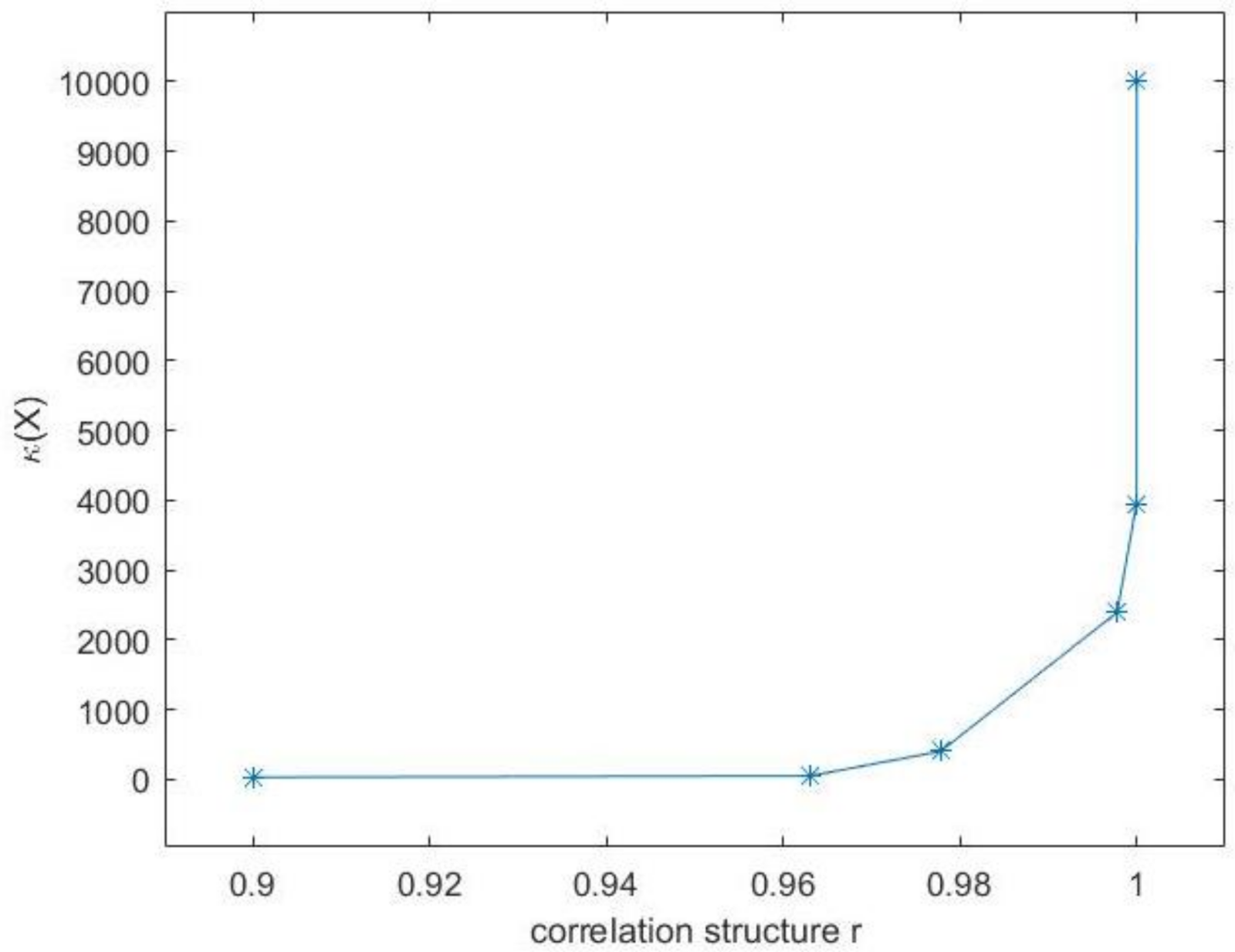
• Estimation of the regression parameter $\mathit{\beta }\in {\mathbb{R}}^{d+1}$.
  From numerical linear algebra point of view, the statistical model (1) can be considered as an underdetermined system. This kind of system has infinitely many solutions. The first way to determine the desired vector $\mathit{\beta }$ is to keep the solution with the minimum norm. This solution is referred to as minimum norm solution (MNS), [1] (p. 264). Another way of solving these problems is based on regularisation techniques. Specifically, these methods allow us to solve a different problem which has a unique solution and thus to estimate the desired vector $\mathit{\beta }$. One of the most popular regularisation methods is Tikhonov regularization, [2]. Another regularization technique which is used is the ${\ell }_p$-${\ell }_q$ regularization, [3,4].
  It is of major importance to decide whether problem (1) can be solved directly in the least squares sense or regularisation is required. Therefore, we describe a way of choosing the appropriate method for solving (1) for design matrices with correlated covariates. For these matrices we study extensively their properties. We prove that as the correlation of the covariates increases, the generalised condition number of the design matrix increases as well and thus the design matrix becomes ill-conditioned.
• To ascertain the most important factors of the statistical model.
  Variable selection is a major issue in solving high-dimensional problems. By means of variable selection we refer to the specification of the important variables (active factors) in the linear regression model, i.e., the variables which play a crucial role in the model. The rest of the variables (inactive factors) can be omitted.
  We deal with the variable selection in supersaturated designs (SSDs) which are fractional factorial designs in which the run size is less than the number of all the main effects. In this class of designs, the columns of X, except the first column, have elements ±1. The symbols 1 and $-1$ are usually utilised to denote the high and low level of each factor, respectively. The correlation of SSDs is usually small, i.e., $r\le 0.5$. The analysis of SSDs is a main issue in Statistics. Many methods for analysing these designs have been proposed. In [5], a Dantzig selector was introduced. Recently, a sure independence screening method has been applied in a model selection method in SSDs [6], and a support vector machine recursive feature elimination method for feature selection [7]. In our study, as we want to retain sparsity in variable selection, we adopt the ${\ell }_p$-${\ell }_q$ regularisation and the SVD principal regression method, [8], in order to determine the most important factors of the statistical model.

In the regression model (1), there is no error setting in the design matrix X which defines the model. It is always considered an unperturbed matrix X with covariates from normal distribution with well determined rank. However, we assume i.i.d. random error $ϵ={({ϵ}_1,{ϵ}_2,\dots ,{ϵ}_n)}^T$, ${ϵ}_i\sim N(0,{\sigma }^2)$ for all $i=1,2,\dots ,n$, incorporated in the model as given from relation (1). Thus, we are having well-posed problems on the set of the data according to the work in [9].

The paper is organised as follows. In Section 2, we briefly present some methods for solving high-dimensional problems. We initially display the MNS and in the sequel we present two regularisation methods. Specifically, Tikhonov regularisation and a general regularisation technique, ${\ell }_p$-${\ell }_q$ regularisation method, are discussed. The described methods are used in estimating the regression parameter $\mathit{\beta }$ of (1) for design matrices with correlated covariates and the results are given in Section 3. These methods can be applied to ill-posed problems as well. Variable selection for SSDs can be found in Section 4. We end up this work with several concluding remarks in Section 5.

2. Methods Overview

In this section, we present some methods for solving high-dimensional problems.

2.1. Minimum Norm Solution

The system (1), which is an underdetermined system, does not have a unique solution. In fact, this underdetermined system has infinitely many solutions, and we are seeking a solution such that its norm is minimised, i.e., the minimum norm solution (MNS) $\underset{\mathit{\beta }\in {\mathbb{R}}^{d+1}}{argmin}{\parallel \mathit{y}-X\mathit{\beta }\parallel }_2^2$, [1] (p. 264). A necessary and sufficient condition for the existence of MNS is given in the following theorem.

Theorem 1.

Let $X\in {\mathbb{R}}^{n\times (d+1)}$ be a high-dimensional matrix, i.e., $n<d$, with $rank\left(X\right)=n$, and ${\mathit{\beta }}^{*}$ be a solution of the underdetermined system $X\mathit{\beta }=\mathit{y}$. Then, ${\mathit{\beta }}^{*}$ is a MNS if and only if ${\mathit{\beta }}^{*}\in Range\left(X^T\right)$.

Proof. 

As ${\mathit{\beta }}^{*}$ is a solution of the underdetermined system $X\mathit{\beta }=\mathit{y}$, we have

$$X{\mathit{\beta }}^{*}=\mathit{y}\iff {\left({\mathit{\beta }}^{*}\right)}^T{X}^T={\mathit{y}}^T.$$

(2)

Let us consider the $QR$ factorisation of $X^T$, i.e.,

$$X^T=QR=Q\left[\begin{array}{c}{R}_1\\ 0_{d+1-n,n}\end{array}\right],$$

where $Q\in {\mathbb{R}}^{(d+1)\times (d+1)}$ is orthogonal and $R_1\in {\mathbb{R}}^{n\times n}$ is upper triangular. Therefore, (2) can be rewritten as

$${\left({\mathit{\beta }}^{*}\right)}^{T}QR={\mathit{y}}^T\iff {\left(Q^T{\mathit{\beta }}^{*}\right)}^{T}R={\mathit{y}}^T.$$

(3)

If we set

$$\mathit{z}=Q^T{\mathit{\beta }}^{*},$$

(4)

then

$$\left(3\right)\iff {\mathit{z}}^{T}R={\mathit{y}}^T\iff R^T\mathit{z}=\mathit{y}.$$

Moreover, we have

$$\begin{array}{c}\hfill \left(4\right)\iff Q^{-1}{\mathit{\beta }}^{*}=\mathit{z}\iff {\mathit{\beta }}^{*}=Q\mathit{z}\iff {\mathit{\beta }}^{*}\in Range\left(Q\right)\iff {\mathit{\beta }}^{*}\in Range\left(X^T\right).\end{array}$$

□

Taking into account the result of the above theorem, we obtain the formula for the MNS ${\mathit{\beta }}^{*}$, which is given by

$${\mathit{\beta }}^{*}=X^T{\left(X{X}^T\right)}^{-1}\mathit{y}.$$

(5)

Formula (5) cannot be used directly for calculating the vector $\mathit{\beta }$, as it is not a stable computation. Therefore, we state the Algorithm 1 for a stable way of calculating the MNS through the singular value decomposition (SVD) of the design matrix X, [1] (p. 265). The operation count for this algorithm is dominated by the computation of the SVD, which requires a cost of $\mathcal{O}\left(n{d}^2\right)$ flops.

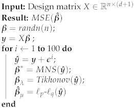
Algorithm 1: Computation of MNS via $SVD$.

Inputs: Design matrix $X\in {\mathbb{R}}^{n\times (d+1)}$, $n<d$, $rank\left(X\right)=n$      Response vector $\mathit{y}\in {\mathbb{R}}^n$  Output: MNS solution ${\mathit{\beta }}^{*}$  − Compute the $SVD$ of X, i.e., ${\displaystyle X=US{V}^T=\sum _{i=1}^n{s}_i{\mathit{u}}_i{\mathit{v}}_i^T}$  − Compute the solution ${\displaystyle {\mathit{\beta }}^{*}=\sum _{i=1}^n{\displaystyle \frac{{\mathit{u}}_i^T\mathit{y}}{s_i}}{\mathit{v}}_i}$

2.2. The Discrete Picard Condition

It is crucial to identify when problem (1) can be directly solved with a satisfactory MNS solution or different ways of handling the solution must be employed. In [10], a criterion for deciding whether a least squares problem can have a satisfactory direct solution or not is proposed. This criterion employs the SVD of the design matrix X and the discrete Picard condition as defined in [11,12]. Let ${\displaystyle X=US{V}^T=\sum _{i=1}^n{s}_i{\mathit{u}}_i{\mathit{v}}_i^T}$ be the SVD of X, where $s_i$ are the singular values of X with corresponding left singular vectors ${\mathit{u}}_i$ and right singular vectors ${\mathit{v}}_i$, $i=1,2,\cdots ,n$. The discrete Picard condition ensures that the solution can be approximated by a regularised solution [13].

Definition 1

(The discrete Picard condition). The discrete Picard condition (DPC) requires that the ratio ${\displaystyle \frac{|c_i|}{s_i}}$ decreases to zero as $i\to n$, i.e.,

$${\displaystyle \frac{|c_i|}{s_i}}\to 0,\mathit{as}i\to n,$$

where $c_i={\mathit{u}}_i^T\mathit{y}$. The DPC implies that the constants $|c_i|$ tend to zero faster than the singular values tend to zero.

Example 1.

Let us now consider design matrices of order $50\times 101$, their columns have same variance ${\sigma }^2$ and same correlation structure r. In particular, we test two design matrices X with $(r,{\sigma }^2)=(0.9,0.25)$ and $(r,{\sigma }^2)=(0.999,1)$. In Figure 1, we display the ratios ${\displaystyle \frac{|c_i|}{s_i}}$ and ${\displaystyle \frac{|{\widehat{c}}_i|}{s_i}}$, which correspond to the noise-free and the noisy problem, $c_i={\mathit{u}}_i^T\mathit{y}$, ${\widehat{c}}_i={\mathit{u}}_i^T\widehat{\mathit{y}}$, $i=1,2,\cdots ,n$, $\widehat{\mathit{y}}=\mathit{y}+ϵ$. If the graphs are close enough the MNS is satisfactory; otherwise, regularisation techniques are necessary for deriving a good approximation of the desired vector β. As we can see in Figure 1, the values of the depicted ratios are very close in the design matrix with $r=0.9$ case whereas in the highly correlated matrix with $r=0.999$ case the ratios differ. This implies that a regularisation method is necessary for the second case.

2.3. Regularisation Techniques

There are cases where the MNS ${\mathit{\beta }}^{*}$ cannot achieve a good approximation of the desired unknown solution $\mathit{\beta }$. As in the linear regression model as described in (1) the design matrix X is always unperturbed, and thus its rank can be a priori known, we can adopt regularisation techniques. In the present section, we present two regularisation methods. In particular, we present the popular Tikhonov regularisation [2] and the ${\ell }_p\text{-}{\ell }_q$ regularisation which has recently received considerable attention [3,4]. Both of these techniques replace the initial problem with another one which is close to the original.

2.3.1. Tikhonov Regularisation

A regularisation method that is widely used is Tikhonov regularisation. The standard form of Tikhonov regularization, which corresponds in linear regression model (1), is given by

$$\underset{\mathit{\beta }\in {\mathbb{R}}^{d+1}}{min}{\{\parallel \mathit{y}-X\mathit{\beta }\parallel }_2^2+{\lambda }^2{\parallel \mathit{\beta }\parallel }_2^2\},$$

(6)

where $\lambda$ is the regularisation parameter. The solution of the penalised least-squares problem (6) is given by the formula

$${\mathit{\beta }}_{\lambda }={(X^{T}X+{\lambda }^2{I}_{d+1})}^{-1}{X}^T\mathit{y}=X^T{(X{X}^T+{\lambda }^2{I}_n)}^{-1}\mathit{y},$$

as it holds the identity ${(X^{T}X+{\lambda }^2{I}_{d+1})}^{-1}{X}^T=X^T{(X{X}^T+{\lambda }^2{I}_n)}^{-1}$. Indeed, we have $X^T(X{X}^T+{\lambda }^2{I}_n)=(X^{T}X+{\lambda }^2{I}_{d+1})X^T\Rightarrow {(X^{T}X+{\lambda }^2{I}_{d+1})}^{-1}{X}^T=X^T{(X{X}^T+{\lambda }^2{I}_n)}^{-1}$.

As we can see, Tikhonov regularisation depends on the regularization parameter $\lambda$. An appropriate method for selecting $\lambda$ leads to the derivation of a satisfactory approximation ${\mathit{\beta }}_{\lambda }$ of the desired regression parameter $\mathit{\beta }$. The error $\mathit{ϵ}$ in the input data for the statistical model that we study follows the standard norm distribution, i.e., $\mathit{ϵ}\sim N({\mathbf{0}}_n,{\sigma }^2{I}_n)$. Therefore, the norm of the error is known, and it is given by ${\parallel \mathit{ϵ}\parallel }_2=\sqrt{n-1}\sigma$. In the case of known error norm, the appropriate method for the selection of the regularisation parameter is the discrepancy principle, which is reported in Algorithm 2 [14] (p. 283). Following also the analysis presented in [9], and due to the uniqueness of $\lambda$ for most reasonable values of $ϵ$ (see, for example, in [15]), we adopt this method for our study.

Algorithm 2: Discrepancy principle.

Inputs: Design matrix $X\in {\mathbb{R}}^{n\times (d+1)}$, $n<d$, $rank\left(X\right)=n$      Response vector $\mathit{y}\in {\mathbb{R}}^n$      Error norm ${\parallel \mathit{ϵ}\parallel }_2=\sqrt{n-1}\sigma$  Output: Regularisation parameter $\lambda$  − Compute the $SVD$ of X, i.e., $X=US{V}^T$  − Set $\mathit{c}=U^T\mathit{y}$  − Choose $\lambda >0$ such that ${\lambda }^4{\mathit{c}}^T{(S+{\lambda }^{2}I)}^{-2}\mathit{c}={\parallel \mathit{e}\parallel }^2$, over a given grid of $\lambda$.

2.3.2. ${\ell }_p$-${\ell }_q$ Regularisation

A more general regularisation technique is the so-called ${\ell }_p$-${\ell }_q$ regularisation [3]. The main idea of this approach is based on the replacement of the minimisation problem ${\parallel \mathit{y}-X\mathit{\beta }\parallel }_2$ by an ${\ell }_p$-${\ell }_q$ minimisation problem of the form

$$\underset{\mathit{\beta }\in {\mathbb{R}}^{d+1}}{min}\{{\displaystyle \frac{1}{p}}{\parallel \mathit{y}-X\mathit{\beta }\parallel }_p^p+\mu {\displaystyle \frac{1}{q}}{\parallel \mathit{\beta }\parallel }_q^q\},$$

(7)

where $\mu >0$ is the regularisation parameter and $0<p,q\le 2$. The solution of the minimisation problem (7) is given by

$${\widehat{\mathit{\beta }}}_{\mu }=\underset{\mathit{\beta }\in {\mathbb{R}}^{d+1}}{argmin}\{{\displaystyle \frac{1}{p}}{\parallel \mathit{y}-X\mathit{\beta }\parallel }_p^p+\mu {\displaystyle \frac{1}{q}}{\parallel \mathit{\beta }\parallel }_q^q\}.$$

(8)

Remark 1.

In case of $p=q=2$, the regularised minimisation problem (7) reduces to Tikhonov regularisation.

Concerning the selection of the regularisation parameter, we choose the optimal value of $\mu$, i.e., the value that minimises the error norm $\parallel {\widehat{\mathit{\beta }}}_{\mu }{-\mathit{\beta }\parallel }_2$ over a given grid of values for $\mu$. Concerning the computational cost, the implementation of the ${\ell }_p$-${\ell }_q$ regularisation requires $\mathcal{O}\left(nd\right)$ flops.

3. Design Matrix with Correlated Covariates

In high-dimensional applications, the design matrix $X=\left[\begin{array}{cccc}\mathbf{1}& {\mathit{x}}_1& \cdots & {\mathit{x}}_d\end{array}\right]$ has correlated covariates ${\mathit{x}}_{\mathit{i}}\sim N({\mathbf{0}}_n,{\sigma }_i^2{I}_n)$, $i=1,\cdots ,d$, where ${\sigma }_i^2$ is the variance of ${\mathit{x}}_{\mathit{i}}$ and the correlation structure is given from the relation

$$r_{ij}=cor({\mathit{x}}_{\mathit{i}},{\mathit{x}}_{\mathbf{j}})={\displaystyle \frac{{\mathit{x}}_{\mathit{i}}^T{\mathit{x}}_{\mathbf{j}}}{\parallel {\mathit{x}}_{\mathit{i}}\parallel \parallel {\mathit{x}}_{\mathbf{j}}\parallel }},i,j=1,\cdots ,d,i\ne j,$$

with $-1\le r_{ij}\le 1$.

Next, we present a thorough investigation of the properties that characterize these matrices.

3.1. Correlated Covariates with Same Variance and Correlation

We initially consider design matrices with correlated covariates which have same variance ${\sigma }^2$ and same correlation r. In the following theorem, we formulate and prove in detail the types for the singular values of the design matrix X. In [16], this case of design matrix is considered and there exists a brief description of the eigenvalues of the matrix $X^{T}X$.

Theorem 2.

Let $X=\left[\begin{array}{cccc}\mathbf{1}& {\mathit{x}}_1& \cdots & {\mathit{x}}_d\end{array}\right]\in {\mathbb{R}}^{n\times (d+1)}$ be a high-dimensional design matrix of full rank whose columns ${\mathit{x}}_i\sim N({\mathbf{0}}_n,{\sigma }^2{I}_n)$, $i=1,2,\cdots ,d$, with correlation structure r. The singular values of the matrix X are

$$s_1=\sqrt{n},s_2=\cdots =s_{n-1}=\sigma \sqrt{(n-1)(1-r)},s_n=\sigma \sqrt{(n-1)\left[\right(d-1)r+1]}.$$

Proof. 

The n singular values of X are the square roots of the n non-zero eigenvalues of $X^{T}X$. Therefore, we compute the matrix $X^{T}X$, i.e.,

$$\begin{array}{ccc}\hfill X^{T}X& =& \left[\begin{array}{ccc}1& \cdots & 1\\ x_{11}& \cdots & x_{n1}\\ ⋮& \ddots & ⋮\\ x_{1d}& \cdots & x_{nd}\end{array}\right]\left[\begin{array}{cccc}1& x_{11}& \cdots & x_{1d}\\ ⋮& ⋮& \ddots & ⋮\\ 1& x_{n1}& \cdots & x_{nd}\end{array}\right]\hfill \end{array}$$

$$\begin{array}{ccc}& =& \left[\begin{array}{cccc}{\displaystyle \sum _{j=1}^{n}1}& {\displaystyle \sum _{j=1}^n{x}_{j1}}& \cdots & {\displaystyle \sum _{j=1}^n{x}_{jd}}\\ {\displaystyle \sum _{j=1}^n{x}_{j1}}& & & \\ ⋮& & {\widehat{X}}^T\widehat{X}& \\ {\displaystyle \sum _{j=1}^n{x}_{jd}}& & & \end{array}\right]=\left[\begin{array}{cccc}n& 0& \cdots & 0\\ 0& & & \\ ⋮& & {\widehat{X}}^T\widehat{X}& \\ 0& & & \end{array}\right],\hfill \end{array}$$

where $\widehat{X}=\left[\begin{array}{ccc}{\mathit{x}}_1& \cdots & {\mathit{x}}_d\end{array}\right]$ and ${\displaystyle \sum _{j=1}^n{x}_{ji}=0}$, $\forall i=1,\cdots ,d$, due to the construction of the design matrix X according to the normal distribution. Therefore, the matrix $X^{T}X$ has one eigenvalue equal to n.

Moreover, we can express the variance ${\sigma }^2$ of each covariate ${\mathit{x}}_i={\left[\begin{array}{cccc}{x}_{1i}& x_{2i}& \cdots & x_{ni}\end{array}\right]}^T$ in terms of vector norms as follows:

$${\sigma }^2={\displaystyle \frac{1}{n-1}}\sum _{j=1}^n{(x_{ji}-\overline{{\mathit{x}}_i})}^2={\displaystyle \frac{1}{n-1}}{\parallel {\mathit{x}}_i-\overline{{\mathit{x}}_i}\parallel }^2,$$

where $\overline{{\mathit{x}}_i}$ denotes the mean value of each ${\mathit{x}}_i$. As the mean value of each ${\mathit{x}}_i$ is zero, we have

$$\begin{array}{c}\hfill {\sigma }^2={\displaystyle \frac{1}{n-1}}\parallel {\mathit{x}}_{\mathit{i}}{\parallel }^2\Rightarrow {\parallel {\mathit{x}}_{\mathit{i}}\parallel }^2=(n-1){\sigma }^2,\forall i=1,\cdots ,d.\end{array}$$

(9)

The submatrix ${\widehat{X}}^T\widehat{X}$ of $X^{T}X$ can be written as

$$\begin{array}{c}\hfill {\widehat{X}}^T\widehat{X}=\left[\begin{array}{cccc}\parallel {\mathit{x}}_1{\parallel }^2& r\parallel {\mathit{x}}_1\parallel \parallel {\mathit{x}}_2\parallel & \cdots & r\parallel {\mathit{x}}_1\parallel \parallel {\mathit{x}}_d\parallel \\ r\parallel {\mathit{x}}_1\parallel \parallel {\mathit{x}}_2\parallel & \parallel {\mathit{x}}_2{\parallel }^2& \cdots & r\parallel {\mathit{x}}_2\parallel \parallel {\mathit{x}}_d\parallel \\ ⋮& ⋮& \ddots & ⋮\\ r\parallel {\mathit{x}}_d\parallel \parallel {\mathit{x}}_1\parallel & r\parallel {\mathit{x}}_d\parallel \parallel {\mathit{x}}_2\parallel & \cdots & \parallel {\mathit{x}}_d{\parallel }^2\end{array}\right]\\ \hfill \stackrel{\left(9\right)}{=}\left[\begin{array}{cccc}(n-1){\sigma }^2& r(n-1){\sigma }^2& \cdots & r(n-1){\sigma }^2\\ r(n-1){\sigma }^2& (n-1){\sigma }^2& \cdots & r(n-1){\sigma }^2\\ ⋮& ⋮& \ddots & ⋮\\ r(n-1){\sigma }^2& r(n-1){\sigma }^2& \cdots & (n-1){\sigma }^2\end{array}\right]\\ \hfill =(n-1){\sigma }^2\left[\begin{array}{cccc}1& r& \cdots & r\\ r& 1& \cdots & r\\ ⋮& ⋮& \ddots & ⋮\\ r& r& \cdots & 1\end{array}\right]=(n-1){\sigma }^2\left[(1-r)I+rJ\right],\end{array}$$

where J is the $d\times d$ matrix with all elements equal to 1. The non-zero eigenvalues of ${\widehat{X}}^T\widehat{X}$ are ${\lambda }_1=(n-1){\sigma }^2(1-r)$ with algebraic multiplicity $n-2$ and ${\lambda }_2=(n-1){\sigma }^2[(d-1)r+1]$ with algebraic multiplicity 1. Therefore, the singular values of X are $s_1=\sqrt{n}$, $s_2=\cdots =s_{n-1}=\sigma \sqrt{(n-1)(1-r)}$, $s_n=\sigma \sqrt{(n-1)\left[\right(d-1)r+1]}$. □

Let us denote by $\kappa \left(X\right)$ the generalised condition number of X, i.e., $\kappa \left(X\right)={\parallel X\parallel }_2·{\parallel X^{†}\parallel }_2$, where $X^{†}=X^T{\left(X{X}^T\right)}^{-1}$ is the pseudoinverse of X, [1] (p. 246). It is known that the generalised condition number can be expressed in terms of the maximum $s_{max}$ and the minimum $s_{min}$ singular value of X as $\kappa \left(X\right)={\displaystyle \frac{s_{max}}{s_{min}}}$, [1] (p. 216).

In Theorem 3, we express the generalised condition number of X in terms of the correlation structure r.

Theorem 3.

Let $X=\left[\begin{array}{cccc}\mathbf{1}& {\mathit{x}}_1& \cdots & {\mathit{x}}_d\end{array}\right]\in {\mathbb{R}}^{n\times (d+1)}$ be a high-dimensional design matrix of full rank whose columns ${\mathit{x}}_i\sim N({\mathbf{0}}_n,{\sigma }^2{I}_n)$, $i=1,2,\cdots ,d$, with correlation structure r. The generalised condition number of X is given by

1. 

$\kappa \left(X\right)=\sqrt{{\displaystyle \frac{n}{(n-1){\sigma }^2(1-r)}}}$, if $r\le {\displaystyle \frac{1}{d-1}}\left({\displaystyle \frac{n}{(n-1){\sigma }^2}}-1\right)$,

2. 

$\kappa \left(X\right)=\sqrt{{\displaystyle \frac{(d-1)r+1}{1-r}}}$, if $\left(r>{\displaystyle \frac{1}{d-1}}\left({\displaystyle \frac{n}{(n-1){\sigma }^2}}-1\right)\mathit{and}{\sigma }^2<{\displaystyle \frac{n}{n-1}}\right)$ or

$\left(r>1-{\displaystyle \frac{n}{(n-1){\sigma }^2}}\mathit{and}{\sigma }^2>{\displaystyle \frac{n}{n-1}}\right)$,

3. 

$\kappa \left(X\right)=\sqrt{{\displaystyle \frac{(n-1){\sigma }^2((d-1)r+1)}{n}}}$, if $r<1-{\displaystyle \frac{n}{(n-1){\sigma }^2}}$.

Proof. 

It is obvious that $s_n=\sigma \sqrt{(n-1)\left[\right(d-1)r+1]}>s_i$, $i=2,\cdots ,n-1$ holds. Therefore, we have to distinguish three cases. The first case is $s_1\ge s_n$, the second case is $s_i<s_1<s_n$ and the last one is $s_1<s_i$.

First case: If $s_1\ge s_n$, then $\kappa \left(X\right)={\displaystyle \frac{s_1}{s_i}}=\sqrt{{\displaystyle \frac{n}{(n-1){\sigma }^2(1-r)}}}$. The restriction $s_1\ge s_n$ can be rewritten as follows:

$$\begin{array}{cc}& n\ge (n-1){\sigma }^2\left((d-1)r+1\right)\\ \hfill \iff & {\displaystyle \frac{n}{(n-1){\sigma }^2}}\ge (d-1)r+1\\ \hfill \iff & {\displaystyle \frac{n}{(n-1){\sigma }^2}}-1\ge (d-1)r\\ \hfill \iff & r\le {\displaystyle \frac{1}{d-1}}\left({\displaystyle \frac{n}{(n-1){\sigma }^2}}-1\right).\end{array}$$

Second case: If $s_i<s_1<s_n$, then $\kappa \left(X\right)={\displaystyle \frac{s_n}{s_i}}=\sqrt{{\displaystyle \frac{(d-1)r+1}{1-r}}}$. The restriction $s_i<s_1<s_n$ can be reformulated as follows:

$$\begin{array}{cc}& (n-1){\sigma }^2(1-r)<n<(n-1){\sigma }^2(dr+1-r)\\ \hfill \iff & \left\{\begin{array}{c}1-r<{\displaystyle \frac{n}{(n-1){\sigma }^2}}\hfill \\ (d-1)r>{\displaystyle \frac{n}{(n-1){\sigma }^2}}-1\hfill \end{array}\right.\iff \left\{\begin{array}{c}r>1-{\displaystyle \frac{n}{(n-1){\sigma }^2}}\hfill \\ r>{\displaystyle \frac{1}{d-1}}\left({\displaystyle \frac{n}{(n-1){\sigma }^2}}-1\right)\hfill \end{array}\right..\end{array}$$

Moreover, we make the check

$$\begin{array}{cc}& {\displaystyle \frac{1}{d-1}}\left({\displaystyle \frac{n}{(n-1){\sigma }^2}}-1\right)<1-{\displaystyle \frac{n}{(n-1){\sigma }^2}}\\ \hfill \iff & n-(n-1){\sigma }^2<(d-1)(n-1){\sigma }^2-n(d-1)\\ \hfill \iff & (n-1){\sigma }^2(1+d-1)>n+nd-n\\ \hfill \iff & {\sigma }^2>{\displaystyle \frac{n}{n-1}}.\end{array}$$

Therefore, we conclude that the generalised condition number $\kappa \left(X\right)$ is equal to $\sqrt{{\displaystyle \frac{(d-1)r+1}{1-r}}}$ if the following relation holds.

$$\begin{array}{ccc}\hfill r>{\displaystyle \frac{1}{d-1}}\left({\displaystyle \frac{n}{(n-1){\sigma }^2}}-1\right)& \mathrm{and}& {\sigma }^2<{\displaystyle \frac{n}{n-1}}\mathrm{or}\hfill \\ \hfill r>1-{\displaystyle \frac{n}{(n-1){\sigma }^2}}& \mathrm{and}& {\sigma }^2>{\displaystyle \frac{n}{n-1}}\hfill \end{array}$$

Third case: If $s_1\le s_i$, then $\kappa \left(X\right)={\displaystyle \frac{s_n}{s_1}}=\sqrt{{\displaystyle \frac{(n-1){\sigma }^2((d-1)r+1)}{n}}}$. This restriction is equivalently written as

$$n<(n-1){\sigma }^2(1-r)\iff {\displaystyle \frac{n}{(n-1){\sigma }^2}}<1-r\iff r<1-{\displaystyle \frac{n}{(n-1){\sigma }^2}}.$$

□

Taking into consideration the derived formulae for the generalised condition number of the design matrix X, we see that if $r\approx 1$ the generalised condition number $\kappa \left(X\right)$ becomes large. A detailed example is presented next.

Example 2.

In this example, we plot the generalised condition number of X as a function of the correlation r. We consider $n=50$, $d=100$ and ${\sigma }^2=2$. In Figure 2, we display $\kappa \left(X\right)$ for correlation $r⟶1$. As we see in Figure 2, as correlation r tends to 1, the generalised condition number $\kappa \left(X\right)$ increases rapidly.

3.2. Highly Correlated Covariates with Different Variance and Correlation

Next, we consider a general and more usual case in which the covariates ${\mathit{x}}_{\mathit{i}}\sim N({\mathbf{0}}_n,{\sigma }_i^2{I}_n)$ of the design matrix X have different variance ${\sigma }_i^2$ and correlation $r_{ij}$, $i,j=1,\dots ,d$. Based on the results presented in [17] for the eigenvalues of the matrix $X^{T}X$, we record analytic formulae for the singular values of X in the following theorem.

Theorem 4.

Let $X=\left[\begin{array}{cccc}\mathbf{1}& {\mathit{x}}_1& \cdots & {\mathit{x}}_d\end{array}\right]\in {\mathbb{R}}^{n\times (d+1)}$ be a high-dimensional design matrix of full rank whose columns ${\mathit{x}}_i\sim N({\mathbf{0}}_n,{\sigma }_i^2{I}_n)$, $i=1,2,\dots ,d$, with highly correlation structure $r_{ij}$. The singular values of the matrix X are

$$s_1=\sqrt{n},s_2=\sqrt{(n-1)\sum _{j=1}^d{\sigma }_i^2+\mathcal{O}\left(\delta \right)},s_3=\cdots =s_n=\sqrt{\mathcal{O}\left(\delta \right)},$$

assuming that $1-r_{ij}=\mathcal{O}\left(\delta \right)$ as $\delta \to 0$.

As we record in Section 3.1, the generalised condition number is equal to the ratio ${\displaystyle \frac{s_{max}}{s_{min}}}$ and in the present case $s_{min}=\mathcal{O}\left(\delta \right)$ considering that $1-r_{ij}=\mathcal{O}\left(\delta \right)$, i.e., highly correlated covariates. Therefore, the value of $\kappa \left(X\right)$ is large and this affects the solution of the corresponding problem.

Remark 2.

As the correlation r increases the generalised condition number $\kappa \left(X\right)$ increases as well. From Theorems 2 and 4 we deduce that the case of highly correlated covariates leads to possible instability and thus regularisation is recommended. This result is confirmed from

Table 1. Results for $X_{5\times 21}$.

r	${\mathit{\sigma }}^2$	Method	$\mathit{\lambda }/\mathit{\mu }$	MSE ($\widehat{\mathit{\beta }}$)
0.5	0.25	MNS		$1.3063\times {10}^{-1}$
		Tikhonov	[1, 10]	$8.3874\times {10}^{-1}$
		${\ell }_{1.8}$-${\ell }_{1.8}$	[${10}^{-7},{10}^{-2}$]	$1.1949\times {10}^{-1}$
0.5	1.0	MNS		$1.3093\times {10}^{-1}$
		Tikhonov	[1, 10]	$8.0127\times {10}^{-1}$
		${\ell }_{1.8}$-${\ell }_{1.8}$	[${10}^{-7},{10}^{-2}$]	$1.2216\times {10}^{-1}$
0.9	0.25	MNS		$5.5782\times {10}^{-1}$
		Tikhonov	[1, 10]	$9.4101\times {10}^{-1}$
		${\ell }_{1.8}$-${\ell }_{1.8}$	[0.1, 10]	$1.2571\times {10}^{-1}$
0.9	1.0	MNS		$6.2096\times {10}^{-1}$
		Tikhonov	[1, 10]	$8.5836\times {10}^{-1}$
		${\ell }_{1.8}$-${\ell }_{1.8}$	[0.1, 10]	$6.0884\times {10}^{-1}$
0.999	0.25	MNS		4.4474
		Tikhonov	[1, 10]	1.774
		${\ell }_{0.1}$-${\ell }_2$	[${10}^{-7},{10}^{-2}$]	$7.3793\times {10}^{-1}$
0.999	1.0	MNS		2.0129
		Tikhonov	[1, 10]	1.0456
		${\ell }_{1.2}$-${\ell }_{1.2}$	[0.1, 10]	$6.8626\times {10}^{-1}$

which is presented in Section 3.3.

3.3. Numerical Implementation

The implementation of the simulation study presented in this section and in Section 4 has been done by using the Julia Programming Language.

Given the high-dimensional design matrix X of order $n\times (d+1)$, the response vector $\mathit{y}$ of order n and the n-vector $\mathit{ϵ}={({ϵ}_1,{ϵ}_2,\cdots ,{ϵ}_n)}^T$ of i.i.d. random errors, ${ϵ}_j\sim N(0,1)$, $j=1,2,\cdots ,n$, we estimate the vector $\mathit{\beta }$ by using the methods which are described in Section 2. We consider design matrices X with correlated covariates and we distinguish the two aforementioned cases. The results for the first case, i.e., the covariates of the design matrices having same correlation r and same variance ${\sigma }^2$, are recorded in Table 1 and

Table 2. Results for $X_{50\times 101}$.

r	${\mathit{\sigma }}^2$	Method	$\mathit{\lambda }/\mathit{\mu }$	MSE ($\widehat{\mathit{\beta }}$)
0.9	0.25	MNS		$4.5894\times {10}^{-1}$
		Tikhonov	[1, 10]	$7.0511\times {10}^{-1}$
		${\ell }_2$-${\ell }_{0.1}$	[${10}^{-7},{10}^{-2}$]	$4.5093\times {10}^{-1}$
0.9	1.0	MNS		$4.8802\times {10}^{-1}$
		Tikhonov	[1, 10]	$6.0754\times {10}^{-1}$
		${\ell }_2$-${\ell }_{0.1}$	[${10}^{-7},{10}^{-2}$]	$4.8614\times {10}^{-1}$
0.999	0.25	MNS		3.5306
		Tikhonov	[1, 10]	1.0022
		${\ell }_2$-${\ell }_{0.1}$	[0.1, 10]	$8.3247\times {10}^{-1}$
0.999	1.0	MNS		1.1970
		Tikhonov	[1, 10]	$9.6625\times {10}^{-1}$
		${\ell }_{1.8}$-${\ell }_{1.8}$	[0.1, 10]	$7.4754\times {10}^{-1}$

. The results for the second case are displayed in

Table 3. Results for $X_{25\times 51}$.

r	${\mathit{\sigma }}^2$	Method	$\mathit{\lambda }/\mathit{\mu }$	MSE ($\widehat{\mathit{\beta }}$)
[0.27, 0.91]	[0.19, 1.17]	MNS		$2.1252\times {10}^{-1}$
		Tikhonov	[1, 10]	$6.2245\times {10}^{-1}$
		${\ell }_{1.8}$-${\ell }_{1.8}$	[0.1, 10]	$9.3163\times {10}^{-2}$
[−0.32, 0.85]	[0.13, 2.32]	MNS		$1.6819\times {10}^{-1}$
		Tikhonov	[1, 10]	$5.9699\times {10}^{-1}$
		${\ell }_{1.8}$-${\ell }_{1.8}$	[0.1, 10]	$1.2632\times {10}^{-1}$
[0.06, 0.91]	[0.42, 1.93]	MNS		$1.1623\times {10}^{-1}$
		Tikhonov	[1, 10]	$5.8305\times {10}^{-1}$
		${\ell }_{1.8}$-${\ell }_{1.8}$	[0.1, 10]	$1.0371\times {10}^{-1}$

.

The implemented simulation scheme is the following. For each design matrix X, a random vector $\mathit{\beta }$ is generated and $\mathit{y}=X\mathit{\beta }$ denotes the noise free response vector. Then, 100 iterations are performed, in each one the response vector is perturbed by noise ${\mathit{ϵ}}^i$ resulting in a noisy response vector $\widehat{\mathit{y}}=\mathit{y}+{ϵ}^i$, $i=1,2,\dots ,100$. Eventually, the regression parameter $\widehat{\mathit{\beta }}$ is computed by using both the MNS given by Algorithm 1 and the regularisation techniques. The quality of the generated approximation solution $\widehat{\mathit{\beta }}$ is assessed by the mean square error (MSE) between $\mathit{\beta }$ and $\widehat{\mathit{\beta }}$ which is given by the formula

$$MSE\left(\widehat{\mathit{\beta }}\right)=E[\parallel \widehat{\mathit{\beta }}-\mathit{\beta }{\parallel }_2^2].$$

In Algorithm 3, we summarise the simulation scheme.

Algorithm 3: Simulation scheme.

In Table 1, Table 2 and Table 3, we present the results of estimating the regression parameter $\mathit{\beta }$ for different orders of the design matrices X. In the two first columns of the tables, the correlation r and the variance ${\sigma }^2$ of the covariates are recorded, respectively. In Table 3, we record the interval in which lies the correlation and the variance. In the third column, the adopted methods are written. Specifically, we record MNS, Tikhonov regularisation and ${\ell }_p$-${\ell }_q$ regularisation technique for different pairs of $(p,q)$. The fourth column contains the used grid of values for the regularisation parameter $\lambda$ or $\mu$ for Tikhonov or ${\ell }_p$-${\ell }_q$ regularisation, respectively. In the last column the $MSE(\widehat{\mathit{\beta }})$ of the derived approximation solutions $\widehat{\mathit{\beta }}$ are recorded.

As we can see in these tables, in the case of highly correlated design matrices, the regularisation is necessary for deriving a good approximation of the desired vector $\mathit{\beta }$. On the other hand, if the correlation of the design matrix is not high, MNS can achieve a fair estimation and a regularisation method does not improve the results, as it is verified by the $MSE(\widehat{\mathit{\beta }})$. Therefore, according to the presented results, for matrices with moderate correlated covariates, regularisation is redundant, as MNS yields adequate results. However, as the correlation between the covariates rises, the regularisation is essential.

Note that in case of design matrices with same variance and correlation $r=0.999$ (Table 1 and Table 2) the regularisation techniques, Tikhonov and ${\ell }_p$-${\ell }_q$, can achieve comparable results. The choice of the pair of parameters $(p,q)$ and the values of the required regularisation parameter play an important role for the efficient implementation of both methods.

4. Variable Selection in SSDs

In this section, we are interested in selecting the active factors of SSDs by using the methods which are described in Section 2. In our comparison, we also include SVD principal regression method which is used in SSDs, and it was proposed in [8]. We briefly refer to this method as SVD regression. The main computational cost of this approach is the evaluation of the SVD.

We measure the effectiveness of these methods through the Type I and Type II error rates. In particular, Type I error measures the cost of declaring an inactive factor to be active and Type II measures the cost of declaring an active effect to be inactive. In our numerical experiments, we consider 500 different realisations of the error $\mathit{ϵ}$ and in the presented tables we record the mean value of Type I, II error rates.

It is worth mentioning that both the MNS and Tikhonov regularisation give that all the factors are active, i.e., Type I $=1$, Type II $=0$, for all the tested SSDs. Therefore, these methods are not suitable for variable selection and we do not include them in the following presented tables.

Example 3

(An illustrative example). In this example, we shall exhibit in detail the performance of each method for a particular problem. For this purpose, we adopt the illustrative example presented in [8], with design matrix

$$X=\left[\begin{array}{cccccccccc}+& -& -& -& -& -& -& -& -& -\\ +& +& +& +& +& +& +& -& -& -\\ +& +& +& +& -& -& -& +& +& +\\ -& +& -& -& +& +& -& +& +& -\\ -& -& +& -& +& -& +& +& -& +\\ -& -& -& +& -& +& +& -& +& +\end{array}\right]=\left[\begin{array}{cccc}{\mathit{x}}_1& {\mathit{x}}_2& \cdots & {\mathit{x}}_{10}\end{array}\right].$$

Then a first column ${\mathit{x}}_0$ with all entries equal to 1 is added to the matrix, which corresponds to the average mean. The simulated data are generated by the model

$$\mathit{y}=5{\mathit{x}}_0+4{\mathit{x}}_2+3{\mathit{x}}_5+ϵ,$$

where $\mathit{ϵ}\sim N({\mathbf{0}}_6,I_6)$. A response vector $\mathit{y}$ obtained by using this model is

$$\mathit{y}={\left[\begin{array}{cccccc}-1.54& 12.02& 6.82& 12.44& 4.62& -1.21\end{array}\right]}^T.$$

The exact regression parameter β and the predicted coefficients by each method are demonstrated below.

$$\begin{array}{c}\hfill \mathit{\beta }={\left[\begin{array}{ccccccccccc}5& 0& 4& 0& 0& 3& 0& 0& 0& 0& 0\end{array}\right]}^T,\\ {\widehat{\mathit{\beta }}}_{MNS}={\left[\begin{array}{ccccccccccc}5.525& 0.1208& 2.4508& 1.1475& 0.1758& 2.0842& 1.1125& -0.1908& 1.2175& 0.2458& -1.0575\end{array}\right]}^T,\hfill \\ {\widehat{\mathit{\beta }}}_{Tik}={\left[\begin{array}{ccccccccccc}4.7237& 0.1114& 2.2592& 1.0578& 0.1621& 1.9212& 1.0255& -0.1759& 1.1223& 0.2266& -0.9748\end{array}\right]}^T,\hfill \\ {\widehat{\mathit{\beta }}}_{{\ell }_2{\ell }_{0.1}}={\left[\begin{array}{ccccccccccc}5.5214& 0.0& 3.9482& 0.0& 0.0& 2.8458& 0.0& 0.0& 0.0& 0.0& 0.0\end{array}\right]}^T,\hfill \\ {\widehat{\mathit{\beta }}}_{SVD}={\left[\begin{array}{ccccccccccc}5.5245& 0.0& 3.901& 0.0& 0.0& 2.801& 0.0& 0.0& 0.0& 0.0& 0.0\end{array}\right]}^T.\hfill \end{array}$$

As we can see from the generated approximation solutions $\widehat{\mathit{\beta }}$, the MNS and Tikhonov regularised solution cannot specify the active factors of the model and completely spoil the sparsity. On the other hand, the ${\ell }_p$-${\ell }_q$ regularisation method and the SVD regression can determine appropriately the active factors of the model.

Example 4

(Williams’ data). We consider the well-known Williams’ dataset (rubber age data) which is reported in

Table 4. The Williams’ data—rubber age data.

1	2	3	4	5	6	7	8	9	10	11	12	13	14	15	16	17	18	19	20	21	22	23	y
+	+	+	-	-	-	+	+	+	+	+	-	-	-	+	+	-	-	+	-	-	-	+	133
+	-	-	-	-	-	+	+	+	-	-	-	+	+	+	-	+	-	-	+	+	-	-	62
+	+	-	+	+	-	-	-	-	+	-	+	+	+	+	+	-	-	-	-	+	+	-	45
+	+	-	+	-	+	-	-	-	+	+	-	-	+	+	-	+	+	+	-	-	-	-	52
-	-	+	+	+	+	-	+	+	-	-	-	-	+	+	+	-	-	+	-	+	+	+	56
-	-	+	+	+	+	+	-	+	+	+	-	+	+	-	+	+	+	+	+	+	-	-	47
-	-	-	-	+	-	-	+	-	+	-	+	+	-	+	+	+	+	+	+	-	-	+	88
-	+	+	-	-	+	-	+	-	+	-	-	-	-	-	-	-	+	-	+	+	+	-	193
-	-	-	-	-	+	+	-	-	-	+	+	-	+	-	+	+	-	-	-	-	+	+	32
+	+	+	+	-	+	+	+	-	-	-	+	+	+	-	+	-	+	-	+	-	-	+	53
-	+	-	+	+	-	-	+	+	-	+	-	+	-	-	-	+	+	-	-	-	+	+	276
+	-	-	-	+	+	+	-	+	+	+	+	-	-	+	-	-	+	-	+	+	+	+	145
+	+	+	+	+	-	+	-	+	-	-	+	-	-	-	-	+	-	+	+	-	+	-	130
-	-	+	-	-	-	-	-	-	-	+	+	+	-	-	-	-	-	+	-	+	-	-	127

. It is a classical dataset of SSDs and it is tested in several works, such as in [8]. As it is written in [8], as the columns 13 and 16 in the original design matrix are identical, the column 13 is removed for executing our numerical experiments. For this dataset we consider two cases, the real case and 3 synthetic cases.

We initially deal with the real case where the design matrix X and the response vector $\mathit{y}$ are given, without the initial knowledge of the desired vector $\mathit{\beta }$. In literature, it is reported that the active factor is ${\mathit{x}}_{15}$. In this case, according to our numerical experiments, the SVD regression and the ${\ell }_p$-${\ell }_q$ regularisation method for $p=0.8$, $q=0.1$ indicate that the factor ${\mathit{x}}_{15}$ is important. In particular, the proposed models, i.e., the coefficients ${\beta }_i$ are given in

Table 5. The selected model for William’s data (real case).

Method	Intercept	${\mathit{x}}_{15}$
${\ell }_{0.8}$-${\ell }_{0.1}$	6.11	−1.13
SVD Regression	102.7857	−36.0341

.

The second case corresponds to 3 synthetic cases, see in [8] and references therein, which are given below. For these simulated cases, we record the results in

Table 6. Results for William’s Data (synthetic cases).

Model	Method	Type I	Type II
Model 1	${\ell }_{1.8}$-${\ell }_{0.8}$	0.23	0.56
	SVD Regression	0.15	0.74
Model 2	${\ell }_{2.0}$-${\ell }_{0.1}$	0.00	0.00
	SVD Regression	0.05	0.00
Model 3	${\ell }_{2.0}$-${\ell }_{0.1}$	0.00	0.27
	SVD Regression	0.07	0.33

. In particular, we compute Type I and II error rates for the described methods. We apply the ${\ell }_p$-${\ell }_q$ regularisation method for $\mu =5$ and the SVD regression for the significance level $a=0.05$. As we notice in this table, both the ${\ell }_p$-${\ell }_q$ regularisation and the SVD regression can select sufficiently the important factors, as we see from the corresponding Type I, II error rates. The first model has the particularity that it includes the interaction of the factors ${\mathit{x}}_5$, ${\mathit{x}}_9$ which does not usually appear in SSDs analysis. The first model is a challenging case for all the methods.

• Model 1: $\mathit{y}\sim N(15{\mathit{x}}_1+8{\mathit{x}}_5-6{\mathit{x}}_9+3{\mathit{x}}_5{\mathit{x}}_9,I_{14})$
• Model 2: $\mathit{y}\sim N(8{\mathit{x}}_1+5{\mathit{x}}_{12},I_{14})$
• Model 3: $\mathit{y}\sim N(10{\mathit{x}}_1+9{\mathit{x}}_2+2{\mathit{x}}_3,I_{14})$

Example 5

(A 3-circulant SSD). In this example, we consider one more SSD, which is also used in [18], and it is recorded in

Table 7. A 3-circulant SSD.

1	2	3	4	5	6	7	8	9	10	11	12	13	14	15	16	17	18	19	20	21
-	-	-	-	-	-	-	+	+	-	-	-	+	-	+	+	+	-	+	+	+
+	+	+	-	-	-	-	-	-	-	+	+	-	-	-	+	-	+	+	+	-
+	+	-	+	+	+	-	-	-	-	-	-	-	+	+	-	-	-	+	-	+
+	-	+	+	+	-	+	+	+	-	-	-	-	-	-	-	+	+	-	-	-
-	-	-	+	-	+	+	+	-	+	+	+	-	-	-	-	-	-	-	+	+
-	+	+	-	-	-	+	-	+	+	+	-	+	+	+	-	-	-	-	-	-
-	-	-	-	+	+	-	-	-	+	-	+	+	+	-	+	+	+	-	-	-
+	+	+	+	+	+	+	+	+	+	+	+	+	+	+	+	+	+	+	+	+

. We test the behaviour of the methods for variable selection by considering three models which can be found in [19] and are given below.

• Model 1: $\mathit{y}\sim N(10{\mathit{x}}_1,I_8)$
• Model 2: $\mathit{y}\sim N(-15{\mathit{x}}_1+8{\mathit{x}}_5-2{\mathit{x}}_9,I_8)$
• Model 3: $\mathit{y}\sim N(-15{\mathit{x}}_1+12{\mathit{x}}_5-8{\mathit{x}}_9+6{\mathit{x}}_{13}-2{\mathit{x}}_{17},I_8)$

The results are presented in

Table 8. Results for 3-circulant SSD.

Model	Method	Type I	Type II
Model 1	${\ell }_{2.0}$-${\ell }_{0.1}$	0.00	0.00
	SVD Regression	0.08	0.00
Model 2	${\ell }_{0.6}$-${\ell }_{1.3}$	0.39	0.13
	SVD Regression	0.08	0.67
Model 3	${\ell }_{1.8}$-${\ell }_{0.8}$	0.39	0.45
	SVD Regression	0.17	0.80

. For the three used models, we apply the ${\ell }_p$-${\ell }_q$ regularisation method for $\mu =5,5.5,0.5$ respectively and the SVD regression for $a=0.25$. According to the presented numerical results, we see that both the ${\ell }_p$-${\ell }_q$ regularisation and the SVD regression can achieve satisfactory Type I and II error rates for the Model 1. On the other hand, for the Model 2 the SVD regression fails to specify the active factors whereas the ${\ell }_p$-${\ell }_q$ regularisation method achieves better Type II error. However, neither of the methods produce fair results for the Model 3. The coefficients of this model are not sufficiently close and this fact affects the behaviour of the methods.

Example 6.

In this example we consider a real data set presented in [20] that deals with moss bags of Rhynchostegium riparioides which were exposed to different water concentrations of 11 trace elements under laboratory conditions. The design matrix X can be found in Table 1 in [20]. We consider the main effects, the second- and third-order interactions of influent factors. Therefore, we have a $67\times 232$ SSD and we can select the important factors applying the ${\ell }_p$-${\ell }_q$ regularisation for $\mu =0.75$ and the SVD regression for significance level $a=0.05$.

From

Table 9. Important elements and interactions.

Method	Main Effects	Second-Order Interactions	Third-Order Interactions
${\ell }_2$-${\ell }_{0.1}$	Fe, Zn	Al/Hg, As/Pb,	Al/As/Mn, Al/Cr/Zn,
		Cd/Mn, Mn/Ni	As/Cd/Fe, As/Cd/Mn,
			Cr/Mn/Zn, Cu/Hg/Mn
			Fe/Hg/Ni, Fe/ Ni/Pb
SVD Regression	Zn	As/Pb, Cd/Mn,
		Fe/Mn, Fe/Zn,
		Mn/Ni, Pb/Zn

, we see that both ${\ell }_2$-${\ell }_{0.1}$ and SVD regression methods identify the main effect Zn as active factor. The second order interactions Cd/Mn, As/Pb and Mn/Ni are also identified as active. These results are in agreement with [20].

5. Conclusions

In the present work, we analysed the properties of design matrices with correlated covariates. Specifically, we derived and proved formulae for the singular values of these matrices and we studied the connection of the generalised condition number with the correlation structure. Moreover, we described some available methods for solving high-dimensional problems. We checked the behaviour of the MNS and the necessity of applying regularisation techniques in estimating the regression parameter $\mathit{\beta }$ in the linear regression model. We concluded that in solving high-dimensional statistical problems the following remarks must be taken into consideration.

• Regularisation should be applied only if the given data set satisfies the discrete Picard condition. In this case, the choice of the regularisation parameter can be uniquely chosen by applying the discrepancy principle method.
• The regression parameter $\mathit{\beta }\in {\mathbb{R}}^{d+1}$ can be satisfactory estimated by the MNS if the design matrix is not highly correlated but in case of highly correlated data matrices we have to adopt regularisation techniques. The quality of the derived estimation $\widehat{\mathit{\beta }}$ of $\mathit{\beta }$ is assessed by the computation of $MSE(\widehat{\mathit{\beta }})$.
• In variable selection, where sparse solutions are needed, SVD regression or ${\ell }_p$-${\ell }_q$ regularisation can be used. When only few factors of the experiment are needed to be specified (maybe only the most important), SVD regression may be preferable since it avoids regularisation and the troublesome procedure of defining the regularisation parameter. The quality of the variable selection which is proposed by the estimation methods is assessed by the evaluation of Type I and II error rates.

In conclusion, the proposed scheme for the selection of the appropriate method for the solution of high-dimensional statistical problems is summarised in the following logical diagram, see Figure 3.

References

- Datta, B.N. Numerical Linear Algebra and Applications, 2nd ed.; SIAM: Philadelphia, PA, USA, 2010. [Google Scholar]
- Tikhonov, A.N. On the solution of ill-posed problems and the method of regularization. Dokl. Akad. Nauk SSSR 1963, 151, 501–504. [Google Scholar]
- Huang, G.; Lanza, A.; Morigi, S.; Reichel, L.; Sgallari, F. Majorization-minimization generalized Krylov subspace methods for ℓp-ℓq optimization applied to image restoration. BIT Numer. Math. 2017, 57, 351–378. [Google Scholar] [CrossRef]
- Buccini, A.; Reichel, L. An ℓ2-ℓq regularization method for large discrete ill-posed problems. J. Sci. Comput. 2019, 78, 1526–1549. [Google Scholar] [CrossRef]
- Candes, E.; Tao, T. The Dantzig Selector: Statistical Estimation When p is much larger than n. Ann. Stat. 2007, 35, 2313–2351. [Google Scholar]
- Drosou, K.; Koukouvinos, C. Sure independence screening for analyzing supersaturated designs. Commun. Stat. Simul. Comput. 2019, 48, 1979–1995. [Google Scholar] [CrossRef]
- Drosou, K.; Koukouvinos, C. A new variable selection method based on SVM for analyzing supersaturated designs. J. Qual. Technol. 2019, 51, 21–36. [Google Scholar] [CrossRef]
- Georgiou, S.D. Modelling by supersaturated designs. Comput. Stat. Data Anal. 2008, 53, 428–435. [Google Scholar] [CrossRef]
- Yagola, A.G.; Leonov, A.S.; Titarenko, V.N. Data errors and an error estimation for ill-posed problems. Inverse Probl. Eng. 2002, 10, 117–129. [Google Scholar] [CrossRef]
- Winkler, J.R.; Mitrouli, M. Condition estimation for regression and feature selection. J. Comput. Appl. Math. 2020, 373, 112212. [Google Scholar] [CrossRef] [Green Version]
- Hansen, P.C. The discrete picard condition for discrete ill-posed problems. BIT 1990, 30, 658–672. [Google Scholar] [CrossRef]
- Hansen, P.C. Rank-Deficient and Discrete Ill-Posed Problems; SIAM: Philadelphia, PA, USA, 1998. [Google Scholar]
- Hansen, P.C. The L-curve and its use in the numerical treatment of inverse problems. In Computational Inverse Problems in Electrocardiology, Advances in Computational Bioengineering 4; WIT Press: Southampton, UK, 2000; pp. 119–142. [Google Scholar]
- Golub, G.H.; Meurant, G. Matrices, Moments and Quadrature with Applications; Princeton University Press: Princeton, NJ, USA, 2010. [Google Scholar]
- Engl, H.W.; Hanke, M.; Neubauer, A. Regularization of Inverse Problems; Kluwer: Dordrecht, The Netherlands, 1996. [Google Scholar]
- Koukouvinos, C.; Lappa, A.; Mitrouli, M.; Roupa, P.; Turek, O. Numerical methods for estimating the tuning parameter in penalized least squares problems. Commun. Stat. Simul. Comput. 2019, 1–22. [Google Scholar] [CrossRef]
- Koukouvinos, C.; Jbilou, K.; Mitrouli, M.; Turek, O. An eigenvalue approach for estimating the generalized cross validation function for correlated matrices. Electron. J. Linear Algebra 2019, 35, 482–496. [Google Scholar] [CrossRef]
- Liu, Y.; Dean, A. k-Circulant supersaturated designs. Technometrics 2004, 46, 32–43. [Google Scholar] [CrossRef]
- Li, R.; Lin, D.K.J. Analysis Methods for Supersaturated Design: Some Comparisons. J. Data Sci. 2003, 1, 249–260. [Google Scholar] [CrossRef]
- Cesa, M.; Campisi, B.; Bizzotto, A.; Ferraro, C.; Fumagalli, F.; Nimis, P.L. A Factor Influence Study of Trace Element Bioaccumulation in Moss Bags. Arch. Environ. Contam. Toxicol. 2008, 55, 386–396. [Google Scholar] [CrossRef] [PubMed]