Input-to-State Stability and Stabilization of Nonlinear Impulsive Positive Systems

Abstract

This paper focuses on the problems of input-to-state stability (ISS) and stabilization for nonlinear impulsive positive systems (NIPS). Using the max-separable ISS Lyapunov function method, a sufficient condition on ISS is given for general NIPS. On that basis, the ISS criteria for linear impulsive positive systems (LIPS) and affine nonlinear impulsive positive systems (ANIPS) are given. Through them, ISS properties can be directly judged from the algebraic and differential characteristics of the systems. Then, utilizing the ISS criteria, state-feedback and impulsive controllers are designed for LIPS and ANIPS, respectively, which make the systems input-to-state stabilizable. Lastly, some numerical examples are given to verify the effectiveness of our results.

1. Introduction

A positive system is a special kind of dynamical system whose state and output variables are non-negative whenever and wherever the initial state and the input variables are non-negative [1]. In recent years, positive systems have been extensively studied and widely used in many fields, such as biology, chemical industries, economics, and sociology. There are many interesting research results from these fields [2,3,4,5,6]. In 1979, the concept of positive systems was first brought forward by Luenberger [7]. On the basis of the tool of a non-negative matrix, Farina first proposed quadratic diagonal Lyapunov functions and obtained the necessary and sufficient conditions on asymptotic stability for positive systems in 2000 [1]. As a result, the study of positive systems was rapidly developed. Both stability [8] and problems of observer design [9], positive filtering [10] and saturation control [11], were studied for positive systems.

The impulse phenomenon is common in engineering applications, which can increase the complexity of system-stability analysis due to the discontinuous system state. In terms of the impact on system stability, impulses are generally divided into three kinds: disturbance, neutral, and stabilizing impulses. Different impulses have different effects on the system, which may hinder convergence or enhance the stability of the considered system. Since the impulsive property and positive constraint lead to abundant dynamic behaviors of an impulsive positive system (IPS), it is necessary and important to investigate the stability and stabilization analysis of IPS. Zhang [12] first established the sufficient criterion of stability for IPS by using a linear copositive Lyapunov function. Briat [13] studied the dwell-time stability and stabilization conditions of linear positive impulsive systems.

Input-to-state stability (ISS) theory plays a vital role in the development of modern nonlinear control theory, especially in the robust stability theory of nonlinear systems. The concept of ISS was proposed by Sontag [14]. Subsequently, its various extensions, such as integral ISS (iISS), finite-time ISS, and stochastic ISS [15,16,17,18], were developed. Many significant results on ISS were reported for various systems, such as continuous dynamical, discrete, sampled-data nonlinear, time-delay, switched, and networked control systems [19,20,21,22,23,24]. For impulsive systems, the ISS problem was also investigated in [25,26,27], with some sufficient conditions provided on the basis of the Lyapunov function method. In addition, for positive systems, there is little research on ISS [28], especially for NIPS. ISS is also an effective tool for stabilization design [29,30,31]. However, for the input-to-state stabilization study of NIPS, the coexistence of positivity restrictions and impulses increases the complexity of input-to-state stabilization analysis. In fact, first, because the state variables of positive systems are always limited in the positive quadrant rather than the whole state space, many methods for general system establishment are not applicable or they are applicable but conservative, which brings great challenges to the ISS analysis for NIPS; second, due to the existence of impulses, the non-negative constraints of the system may be destroyed.

In this paper, the ISS problem of NIPS is studied for the first time, with some criteria on ISS and input-to-state stabilization being provided. On the basis of the max-separable ISS Lyapunov function method, a sufficient condition on ISS for general NIPS is provided in which the two following situations of NIPS are included: (1) the continuous dynamic is stable but the impulsive effect is unstable; (2) the impulsive dynamic is stable but the continuous dynamic is unstable. For LIPS and ANIPS, some ISS criteria are also given. From them, corresponding ISS properties can be judged directly from the algebraic and differential characteristics of the systems. On the basis of the ISS criteria for LIPS and ANIPS, state-feedback and impulsive controllers were designed, respectively, which make the systems input-to-state stabilizable. Numerical examples are given to verify the validity of our proposed results.

The remainder of this paper is organized as follows: in Section 2, the impulsive positive system is formulated, and some notations and definitions are given. In Section 3, after providing a sufficient condition on ISS for general NIPS by the max-separable ISS Lyapunov function method, some ISS criteria are also given for LIPS and ANIPS. In Section 4, for input-to-state stabilization problems, both state-feedback and impulsive controllers were designed and are outlined for LIPS and ANIPS, respectively. In Section 5, three numerical examples are provided to illustrate the proposed results, and the conclusion follows in Section 6.

2. Preliminaries

Notations: Let $\mathbb{R}$, ${\mathbb{R}}_{+}$, $\mathbb{N}$ and ${\mathbb{N}}_{+}$ denote the sets of all real, non-negative real, and natural numbers, and natural numbers excluding zero, respectively. ${\mathbb{R}}^n$ and ${\mathbb{R}}^{n\times m}$ denote the n- and $n\times m$-dimensional real spaces, respectively. Positive orthant ${\mathbb{R}}_{+}^n$ in ${\mathbb{R}}^n$ is set $\{x={(x_1,\cdots ,x_n)}^T\in {\mathbb{R}}^n:x_i\ge 0,\forall i\}$, where superscript T denotes the transpose. A real matrix $A=\left(a_{ij}\right)\in {\mathbb{R}}^{n\times n}$ is called a Metzler matrix if and only if its off-diagonal entries are non-negative: $a_{ij}\ge 0$, $\forall i\ne j$. For vectors $x,y\in {\mathbb{R}}^n$, we write: $x\succ y$$(x\prec y)$ if $x_i>y_i$$\left(x_i<y_i\right)$ for $i\in {\mathcal{I}}_n=:\{1,2,\cdots ,n\}$; $x⪰y$$(x⪯y)$ if $x_i\ge y_i$ $\left(x_i\le y_i\right)$ for $i\in {\mathcal{I}}_n$; $x>y$$(x<y)$ if $x⪰y$$(x⪯y)$ and $x\ne y$. ${\mathbf{1}}_n\in {\mathbb{R}}^n$ refers to the vector with all elements of it being 1. The p-norm on ${\mathbb{R}}^n$ is denoted by ${\parallel ·\parallel }_p$. When $p=2$, p is often omitted. The max-norm is denoted as ${\parallel ·\parallel }_{\infty }$. $\mathcal{V}:=int{\mathbb{R}}_{+}^n$ refers to the interior of ${\mathbb{R}}_{+}^n$ which means set $\{x\in {\mathbb{R}}_{+}^n:x_i>0,\forall i\in {\mathcal{I}}_n\}$. Given a vector $v\in \mathcal{V}$, the weighted $l_{\infty }$ norm is defined by ${\parallel x\parallel }_{\infty }^v={max}_{1\le i\le n}\frac{|x_i|}{v_i}$.

A continuous function $\gamma :[0,\infty )\to [0,\infty )$ is of a class $\mathcal{K}$ if $\gamma$ is strictly increasing and $\gamma (0)=0$. If $\gamma$ is also unbounded, then $\gamma$ is of class ${\mathcal{K}}_{\infty }$. A function $\beta :[0,\infty )\times [0,\infty )\to [0,\infty )$ is of class $\mathcal{KL}$ if for fixed $t\ge 0$ the function $\beta (·,t)$ is of class $\mathcal{K}$, and for fixed $s\ge 0$ the function $\beta (s,·)$ is decreasing with ${lim}_{t\to \infty }\beta (s,t)=0$.

In this paper, we consider the following nonlinear impulsive system with disturbance:

$$\left\{\begin{array}{cc}\dot{x}(t)=f(x(t),w(t)),\hfill & t\ge t_0,t\ne t_k;\hfill \\ x(t_k)=h(x(t_k^{-}),w(t_k)),\hfill & k\in {\mathbb{N}}_{+},\hfill \end{array}\right.$$

(1)

where $x\in {\mathbb{R}}_{+}^n$ is the system state, $w\in {\mathcal{L}}_{\infty }^m$ is the disturbance input, ${\mathcal{L}}_{\infty }^m$ denotes the set of all measurable and locally essentially bounded disturbance input $w\in {\mathbb{R}}_{+}^m$ on $[t_0,\infty )$ with norm as follows:

$${\parallel w\parallel }_{\mathrm{E}}=ess\underset{t\ge t_0}{sup}{\{\parallel w(t)\parallel }_{\infty }\}.$$

$f:{\mathbb{R}}_{+}^n\times {\mathbb{R}}_{+}^m\to {\mathbb{R}}^n$ satisfies $f(0,0)=0$; initial data $x_0={(x_{01},\cdots ,x_{0n})}^T\in {\mathbb{R}}_{+}^n$; $h:{\mathbb{R}}_{+}^n\times {\mathbb{R}}_{+}^m\to {\mathbb{R}}_{+}^n$ is a non-negative function with $h(0,0)=0$; disturbance input function $w(·):[t_0,\infty )\to \mathcal{U}\subset {\mathbb{R}}_{+}^m$ is essentially bounded; $t_k$ denotes the impulsive jump instant, and discrete time set ${\left\{t_k\right\}}_{k=1}^{\infty }$ satisfies $t_1<t_2<\cdots <t_{k-1}<t_k<\cdots$ and ${lim}_{k\to \infty }{t}_k\to \infty$, where $t_1>t_0$, initial time $t_0\ge 0$ and impulsive interval $t_k-t_{k-1}$ are finite. When time instant $t=t_k$, state variable x immediately “jumps” from $x(t_k^{-})$ to $x(t_k)=h(x(t_k^{-}),w(t_k))$.

For convenience, we introduce some definitions and proposition for system (1) as follows.

Definition 1.

For any given constants $T_a>0$ and positive integer $N_0$, let $N_{\sigma }(t,s)$ denote the number of impulsive times of impulse sequence $\sigma ={\left\{t_k\right\}}_{k=1}^{\infty }$ on interval $[s,t),\forall t>s\ge t_0$, and let the following hold [32]:

$$\ell [T_a,N_0]:=\left\{\sigma :\frac{t-s}{T_a}-N_0\le N_{\sigma }(t,s)\le \frac{t-s}{T_a}+N_0,\forall t\ge s\ge t_0\right\},$$

(2)

then $T_a$ is called the average impulsive interval of σ, and $N_0$ is called the chatter bound.

Remark 1.

For system (1), two kinds of impulses are mainly considered. When system function f is stable, but impulses could probably destroy stability, we must require that impulses do not happen too frequently, so the number of impulses is limited to $N_{\sigma }(t,s)\le \frac{t-s}{T_a}+N_0$. When impulse dynamics $x(t_k)=h(x(t_k^{-}),w(t_k))$ are stable with respect to w, but system function f could potentially destroy stability, so we require more impulses to occur and the value of $T_a$ cannot be too large; the number of impulses is limited to $N_{\sigma }(t,s)\ge \frac{t-s}{T_a}-N_0$.

Definition 2.

[1] A nonlinear impulsive system (1) is said to be positive if, for any initial condition $x_0⪰0$, we have $x(t)⪰0$ for any $t\ge t_0$.

Definition 3.

[33] Function f in system (1) is cooperative if the following is true:

$$\begin{array}{ccc}\hfill \frac{\partial f_i}{\partial x_j}(x,w)& \ge & 0,\forall x\in \mathcal{V},\forall w\in \mathcal{W},\forall i\ne j,\hfill \\ \hfill \frac{\partial f_i}{\partial w_j}(x,w)& \ge & 0,\forall x\in {\mathbb{R}}_{+}^n,\forall w\in \mathcal{W}\hfill \end{array}$$

where $\mathcal{V}:=int{\mathbb{R}}_{+}^n$, $\mathcal{W}=int\mathcal{U}$.

Proposition 1.

A nonlinear impulsive system (1) is positive if f is cooperative and h is non-negative.

Proof. 

For system (1) with initial condition $x_0⪰0$, according to analysis in [34], because f is cooperative, one has $x(t)⪰0$ for $t\in [t_0,t_1)$. When $t=t_1$, $x(t_1)=h(x(t_1^{-}),w(t_1))$. Since h is non-negative, one has $x(t_1)⪰0$. For $t\in [t_1,t_2)$, and system (1) with initial state $x(t_1)⪰0$, iteratively, one has $x(t)⪰0$ for $t\in [t_1,t_2)$; generally, for all $t\in [t_k,t_{k+1})(k\in \mathbb{N})$, $x(t)⪰0$. So, $x(t)⪰0$ for all $t\ge t_0$, and system (1) is positive. □

In this paper, the ISS properties of nonlinear impulsive positive systems (NIPS) are considered. For the ISS study of NIPS, the definitions of ISS and max-separable ISS Lyapunov function are first introduced.

Definition 4.

[28] NIPS (1) is said to be input-to-state stable (ISS) if there exist scalar functions $\beta \in \mathcal{K}\mathcal{L}$ and $\gamma \in \mathcal{K}$ such that the following is true:

$$\begin{array}{c}\hfill x(t)⪯\beta \left(\underset{i\in {\mathcal{I}}_n}{max}\left\{x_{0i}\right\},t-t_0\right){\mathbf{1}}_n+{\gamma (\parallel w\parallel }_{\mathrm{E}}){\mathbf{1}}_n.\end{array}$$

From the properties of $\mathcal{K}\mathcal{L}$ functions [35] and Remark 1 in [28], if NIPS (1) is ISS, it is also ISS in the sense of the $l_{\infty }$, $l_1$ and $l_2$-norm.

Definition 5.

For NIPS (1), a locally Lipschitz positive definite radially unbounded function,

$$V(x)=\underset{i\in {\mathcal{I}}_n}{max}\left\{V_i\left(x_i\right)\right\},$$

(3)

with function $V_i$: ${\mathbb{R}}_{+}\to {\mathbb{R}}_{+}$ is a max-separable ISS Lyapunov function if there are functions ${\alpha }_1$, ${\alpha }_2$, χ of class $\mathcal{K}$ and rate coefficients $c,d\in \mathbb{R}$ such that, for all $i\in {\mathcal{I}}_n$, the following is true:

$$\begin{array}{c}\hfill {\alpha }_1(x_i)\le V_i(x_i)\le {\alpha }_2(x_i),\end{array}$$

(4)

and

$$\begin{array}{ccc}\hfill & V(x)\ge {\chi (\parallel w\parallel }_{\mathrm{E}})\Rightarrow D^{+}V(x)\le -cV(x),& \end{array}$$

(5)

$$\begin{array}{ccc}& V(h(x,w))\le e^{-d}V(x),& \hfill \end{array}$$

(6)

where the upper-right Dini derivative $D^{+}V(x)$ is given by the following:

$$D^{+}V(x)=\underset{i\in \mathcal{J}(x)}{max}\left\{\frac{\partial V_j}{\partial x_j}{f}_j(x)\right\},$$

(7)

$\mathcal{J}(x)$ denotes the set of indices for which the maximum in (3) is attained, i.e., the following:

$$\mathcal{J}(x)=\{j\in {\mathcal{I}}_n|V_j(x_j)=V(x)\}.$$

3. ISS of Nonlinear Impulsive Positive Systems

In this section, using the max-separable ISS Lyapunov function method, we state and prove the following ISS criterion for NIPS.

Theorem 1.

For positive system (1) (uniform ISS), if there is a candidate max-separable ISS Lyapunov function $V(x)$ in the form of (3), system (1) is ISS for all impulse sequences $\sigma \in {\ell }_0[T_a,N_0]=\{\sigma \in \ell [T_a,N_0]:\frac{d}{T_a}+c>0\}$.

Proof. 

Define set $\mathcal{Q}=\{x\in {\mathbb{R}}_{+}^n\mid {V(x)<\chi (\parallel w\parallel }_{\mathrm{E}})\}$. The whole proof is performed in two cases: $x_0\in {\mathcal{Q}}^c$ and $x_0\in \mathcal{Q}\backslash \left\{0\right\}$. Let ${\check{t}}_1\in [t_0,\infty )$ denote a time at which the trajectory enters set $\mathcal{Q}$ for the first time.

Case 1.$x_0\in {\mathcal{Q}}^c$. In this case, for any $t\in [t_0,{\check{t}}_1)$, $V(x)\ge \chi (\parallel w{\parallel }_{\mathrm{E}})$. In view of (5), we have the following:

$$\begin{array}{c}\hfill D^{+}V(x)\le -cV(x),t\in \left[t_0,{\check{t}}_1\right).\end{array}$$

From (6), $V(x(t_k))\le e^{-d}V(x(t_k^{-}))$. Thus we have the following:

$$\begin{array}{c}\hfill V(x(t))\le e^{-dN(t,t_0)-c(t-t_0)}V(x(t_0)),t\in \left[t_0,{\check{t}}_1\right).\end{array}$$

(8)

From (2) and (8), we obtain that, if $d>0$,

$$\begin{array}{ccc}\hfill V(x(t))& \le & e^{-d(\frac{t-t_0}{T_a}-N_0)-c(t-t_0)}V(x(t_0))\hfill \\ & =& e^{d{N}_0}{e}^{-(\frac{d}{T_a}+c)(t-t_0)}V(x(t_0)),t\in \left[t_0,{\check{t}}_1\right);\hfill \end{array}$$

if $d<0$,

$$\begin{array}{ccc}\hfill V(x(t))& \le & e^{-d(\frac{t-t_0}{T_a}+N_0)-c(t-t_0)}V(x(t_0))\hfill \\ & =& e^{-d{N}_0}{e}^{-(\frac{d}{T_a}+c)(t-t_0)}V(x(t_0)),t\in \left[t_0,{\check{t}}_1\right).\hfill \end{array}$$

In conclusion, the following holds:

$$\begin{array}{c}\hfill V(x(t))\le \tilde{M}{e}^{-(\frac{d}{T_a}+c)(t-t_0)}V(x(t_0)),t\in \left[t_0,{\check{t}}_1\right),\end{array}$$

where $\tilde{M}=max\{e^{d{N}_0},e^{-d{N}_0}\}$.

According to the definition of max-separable ISS Lyapunov function and the properties of $\mathcal{K}$ functions, the following holds:

$$\begin{array}{c}\hfill {\alpha }_1\left(\underset{i\in {\mathcal{I}}_n}{max}\left\{x_i\right\}\right)=\underset{i\in {\mathcal{I}}_n}{max}\left\{{\alpha }_1\left(x_i\right)\right\}\le \underset{i\in {\mathcal{I}}_n}{max}\left\{V_i\left(x_i\right)\right\}=V(x).\end{array}$$

(9)

Then, we have the following:

$$\begin{array}{ccc}\hfill {\alpha }_1(\underset{i\in {\mathcal{I}}_n}{max}\left\{x_i\right\})& \le & \tilde{M}{e}^{-(\frac{d}{T_a}+c)(t-t_0)}V(x(t_0))\hfill \\ & \le & \tilde{M}{e}^{-(\frac{d}{T_a}+c)(t-t_0)}{\alpha }_2(\underset{i\in {\mathcal{I}}_n}{max}\left\{x_{0i}\right\}),t\in \left[t_0,{\check{t}}_1\right).\hfill \end{array}$$

So,

$$\begin{array}{ccc}\hfill x(t)& ⪯& {\alpha }_1^{-1}(\tilde{M}{e}^{-(\frac{d}{T_a}+c)(t-t_0)}{\alpha }_2(\underset{i\in {\mathcal{I}}_n}{max}\left\{x_{0i}\right\})){\mathbf{1}}_n\hfill \\ & :=& \beta (\underset{i\in {\mathcal{I}}_n}{max}\left\{x_{0i}\right\},t-t_0){\mathbf{1}}_n,t\in \left[t_0,{\check{t}}_1\right),\hfill \end{array}$$

(10)

where $\beta \in \mathcal{KL}$ can be known from Lemma 4.2 in [35].

Let us now turn our attention to interval $[{\check{t}}_1,\infty )$. At ${\check{t}}_1$, the system state goes into set $\mathcal{Q}$ for the first time. If $d\ge 0$, $0<e^{-d}\le 1$, from Condition (6), the impulsive effect is stabilizing or neutral. After time ${\check{t}}_1$, due to the stabilizing or neutral impulses and condition (5), system states always stay in set $\mathcal{Q}$, i.e., $V(x)<\chi (\parallel w{\parallel }_{\mathrm{E}})$. So, from (9), we have the following:

$$\begin{array}{c}\hfill \begin{array}{cc}\hfill x(t)& ⪯{\alpha }_1^{-1}\circ {\chi (\parallel w\parallel }_{\mathrm{E}}){\mathbf{1}}_n:={\gamma }_1{(\parallel w\parallel }_{\mathrm{E}}){\mathbf{1}}_n,t\in [{\check{t}}_1,\infty ),\hfill \end{array}\end{array}$$

where ${\gamma }_1={\alpha }_1^{-1}\circ \chi \in \mathcal{K}$ can be known from Lemma 4.2 in [35]. Combining this with (10), we obtain the following:

$$\begin{array}{c}\hfill x(t)⪯\beta (\underset{i\in {\mathcal{I}}_n}{max}\left\{x_{0i}\right\},t-t_0){\mathbf{1}}_n+{\gamma }_1{(\parallel w\parallel }_{\mathrm{E}}){\mathbf{1}}_n,t\in [t_0,\infty ).\end{array}$$

Otherwise, if $d<0$, the disturbance effect is performed for the impulses. Even if the system state goes into set $\mathcal{Q}$, it can also go out due to the disturbance effect of the impulses. Let ${\widehat{t}}_1:=inf\{t>{\check{t}}_1:V(x(t))\ge {\chi (\parallel w\parallel }_{\mathrm{E}})\}\le \infty$. From the above result, $V(x(t))<\chi (\parallel w{\parallel }_{\mathrm{E}})$ holds when $t\in \left[{\check{t}}_1,{\widehat{t}}_1\right)$. From (9), we obtain the following:

$$\begin{array}{c}\hfill \begin{array}{cc}\hfill x(t)& ⪯{\alpha }_1^{-1}\circ {\chi (\parallel w\parallel }_{\mathrm{E}}){\mathbf{1}}_n={\gamma }_1{(\parallel w\parallel }_{\mathrm{E}}){\mathbf{1}}_n,t\in [{\check{t}}_1,{\widehat{t}}_1).\hfill \end{array}\end{array}$$

(11)

Next, let ${\check{t}}_2:=min\{t>{\widehat{t}}_1{:V(x(t))<\chi (\parallel w\parallel }_{\mathrm{E}})\}\le \infty$. For time ${\widehat{t}}_1$, it is the first time after ${\check{t}}_1$ such that $V(x(t))\ge \chi (\parallel w{\parallel }_{\mathrm{E}})$. From (5), the reason for $V(x({\widehat{t}}_1))\ge {\chi (\parallel w\parallel }_{\mathrm{E}})$ just comes from the impulsive effect. So, the ${\widehat{t}}_1$ is also an impulsive instant. Repeating the argument used to establish (10), with ${\widehat{t}}_1$ in place of $t_0$, we obtain the following:

$$\begin{array}{ccc}\hfill V(x(t))& \le & \mu \tilde{M}V(x({\widehat{t}}_1))\le \tilde{M}{e}^{-(\frac{d}{T_a}+c)(t-{\widehat{t}}_1^{-})}{e}^{-d}V(x({\widehat{t}}_1^{-}))\hfill \\ & \le & \tilde{M}{e}^{-(\frac{d}{T_a}+c)(t-{\widehat{t}}_1^{-})}{e}^{-d}{\chi (\parallel w\parallel }_{\mathrm{E}})\hfill \\ & \le & \tilde{M}{e}^{-d}{\chi (\parallel w\parallel }_{\mathrm{E}}),t\in \left[{\widehat{t}}_1,{\check{t}}_2\right).\hfill \end{array}$$

From (9), we conclude the following:

$$\begin{array}{c}\hfill {\alpha }_1\left(\underset{i\in {\mathcal{I}}_n}{max}\left\{x_i\right\}\right)\le \tilde{M}{e}^{-d}{\chi (\parallel w\parallel }_{\mathrm{E}}),t\in [{\widehat{t}}_1,{\check{t}}_2).\end{array}$$

So,

$$\begin{array}{c}\hfill \begin{array}{cc}\hfill x(t)& ⪯{\alpha }_1^{-1}(\tilde{M}{e}^{-d}{\chi (\parallel w\parallel }_{\mathrm{E}})){\mathbf{1}}_n:={\gamma }_2{(\parallel w\parallel }_{\mathrm{E}}){\mathbf{1}}_n,t\in [{\widehat{t}}_1,{\check{t}}_2),\hfill \end{array}\end{array}$$

(12)

where ${\gamma }_2(·)={\alpha }_1^{-1}(\tilde{M}{e}^{-d}\chi (·))\in \mathcal{K}$ can be known from Lemma 4.2 in [35].

From (10), (11) and (12), iteratively, we obtain $x(t)⪯\beta ({max}_{i\in {\mathcal{I}}_n}\left\{x_{0i}\right\},t-t_0){\mathbf{1}}_n$ for $t\in \left[t_0,{\check{t}}_1\right)$; $x(t)⪯{\gamma }_1{(\parallel w\parallel }_{\mathrm{E}}){\mathbf{1}}_n$ for $t\in \left[{\check{t}}_1,{\widehat{t}}_1\right)\cup \left[{\check{t}}_2,{\widehat{t}}_2\right)\cup \cdots \cup \left[{\check{t}}_k,{\widehat{t}}_k\right)\cup \cdots$; $x(t)⪯{\gamma }_2{(\parallel w\parallel }_{\mathrm{E}}){\mathbf{1}}_n$ for $t\in \left[{\widehat{t}}_1,{\check{t}}_2\right)\cup \left[{\widehat{t}}_2,{\check{t}}_3\right)\cup \cdots \cup \left[{\widehat{t}}_k,{\check{t}}_{k+1}\right)\cup \cdots$. Therefore, the following holds:

$$\begin{array}{c}\hfill x(t)⪯\beta (\underset{i\in {\mathcal{I}}_n}{max}\left\{x_{0i}\right\},t-t_0){\mathbf{1}}_n+{\gamma (\parallel w\parallel }_{\mathrm{E}}){\mathbf{1}}_n,t\in [t_0,\infty ),\end{array}$$

where $\gamma =max\{{\gamma }_1,{\gamma }_2\}$.

Case 2.$x_0\in \mathcal{Q}\backslash \left\{0\right\}$. In this case, ${\check{t}}_1=t_0$. When $t>t_0$, from the proof of Case 1, we obtain the following:

$$\begin{array}{c}\hfill x(t)⪯\beta (\underset{i\in {\mathcal{I}}_n}{max}\left\{x_{0i}\right\},t-t_0){\mathbf{1}}_n+{\gamma (\parallel w\parallel }_{\mathrm{E}}){\mathbf{1}}_n,t\in (t_0,\infty ).\end{array}$$

when $t=t_0$, by the definition of set $\mathcal{Q}$ and the definition of $\gamma$, we obtain the following:

$$\begin{array}{c}\hfill x(t)⪯{\gamma (\parallel w\parallel }_{\mathrm{E}}){\mathbf{1}}_n⪯\beta (\underset{i\in {\mathcal{I}}_n}{max}\left\{x_{0i}\right\},t-t_0){\mathbf{1}}_n+{\gamma (\parallel w\parallel }_{\mathrm{E}}){\mathbf{1}}_n,t\in [t_0,\infty ).\end{array}$$

In all, system (1) is ISS for all impulse sequences $\sigma \in {\ell }_0[T_a,N_0]$. □

Remark 2.

For the study of nonlinear positive systems, the influence of impulses is considered for the first time. The max-separable Lyapunov function method is combined with the average dwell-time method for the study of positive systems. Using them, Theorem 1 provides the stability criteria for NIPS.

Remark 3.

System (1) is affected by both impulses and perturbation input. From the above proof, upper bound ${\gamma }_1{(\parallel w\parallel }_{\mathrm{E}})$ of the solution introduced by the perturbation input may be continuously destroyed due to the action of the impulses. Here, under the general premise of the system positivity requirement, we give a “new upper bound”, which is related to both the impulses and the perturbation input by discussing the time periods of the impulses in sections.

Remark 4.

The “new upper bound” is introduced because of the influence of impulses. By defining set $\mathcal{Q}=\{x\in {\mathbb{R}}_{+}^n\mid V(x)<\chi (\parallel w\parallel )\}$, ${\mathbb{R}}_{+}^n$ can be divided into two parts: ${\mathcal{Q}}^c$ and $\mathcal{Q}$. ${\gamma }_1(\parallel w\parallel ):={\alpha }_1^{-1}\circ \chi (\parallel w\parallel )$ is the “old upper bound”. Without impulses, this bound can be seen as the ultimate bound of the system states. However, due to the disturbance effect of the impulses (when $d<0$), even if the system states enter set $\{x:x⪯{\gamma }_1(\parallel w\parallel )1_n\}$, it may break through the “old upper bound”. From our derivation, the “new upper bound” $\gamma =max\{{\gamma }_1,{\gamma }_2\}$ can be used as an “ultimate bound” of the system states of the NIPS.

Remark 5.

In Theorem 1, two kinds of impulses are mainly considered:

When $d<0$, it must necessarily be with $c>0$, and the value of $T_a$ cannot be too small for Theorem 1 to hold. In this case, (5) implies that system dynamics $\dot{x}=f(x,w)$ are ISS with respect to w, but impulses can probably destroy ISS, and we must require that impulses do not happen very often. The number of impulses is limited to the following:

$$\begin{array}{c}\hfill N_{\sigma }(t,s)\le \frac{t-s}{T_a}+N_0,\forall t\ge s\ge t_0.\end{array}$$

When $d>0$, (6) implies that the impulse dynamics $x(t_k)=h(x(t_k^{-}),w(t_k))$ are ISS with respect to w. When $c<0$, the system dynamics can potentially destroy ISS. So, we must require more impulses to occur and the value of $T_a$ cannot be too large for Theorem 1 to hold. The number of impulses is limited to the following:

$$\begin{array}{c}\hfill N_{\sigma }(t,s)\ge \frac{t-s}{T_a}-N_0,\forall t\ge s\ge t_0.\end{array}$$

Now, consider the NIPS (1) with $f(x,w)=Ax+w$ and $h(x,w)=\mathsf{\Gamma }x(t_k^{-})$, where $A=(a_{ij})\in {\mathbb{R}}^{n\times n}$, $\mathsf{\Gamma }=({\gamma }_{ij})\in {\mathbb{R}}_{+}^{n\times n}$ are the constant matrices, and the function $w:[t_0,\infty )\to {\mathbb{R}}_{+}^n$ is the disturbance input. Then, NIPS (1) reduces to a linear impulsive positive system (LIPS) as follows:

$$\left\{\begin{array}{cc}\dot{x}(t)=Ax(t)+w(t),\hfill & t\ge t_0,t\ne t_k;\hfill \\ x(t_k)=\mathsf{\Gamma }x(t_k^{-}),\hfill & k\in {\mathbb{N}}_{+}.\hfill \end{array}\right.$$

(13)

For LIPS (13), the following proposition can be obtained by the max-separable ISS Lyapunov function method.

Proposition 2.

For the LIPS (13), suppose that A is a Metzler matrix, and that there exist numbers ${\epsilon }_0\in \mathbb{R}$, ${\xi }_0>0$ and vector $v\succ 0$ such that for any $i\in {\mathcal{I}}_n$, the following holds:

$$\begin{array}{c}\hfill a_{ii}+\sum _{j=1,j\ne i}^n{a}_{ij}\frac{v_j}{v_i}\le -{\epsilon }_0,{\gamma }_{ii}+\sum _{j=1,j\ne i}^n{\gamma }_{ij}\frac{v_j}{v_i}\le {\xi }_0,\end{array}$$

i.e.,

$$\begin{array}{c}\hfill Av+{\epsilon }_{0}v⪯0,\mathsf{\Gamma }v-{\xi }_{0}v⪯0.\end{array}$$

Then, system (13) is ISS for all $\sigma \in {\ell }_0[T_a,N_0]=\{\sigma (·)\in \ell [T_a,N_0]:\frac{ln{\xi }_0}{T_a}-\frac{{\epsilon }_0}{2}<0\}$.

Proof. 

See Appendix A. □

Consider an affine nonlinear impulsive positive system (ANIPS) as follows:

$$\left\{\begin{array}{cc}\dot{x}(t)=f(x(t))+g(x(t))w(t),\hfill & t\ge t_0,t\ne t_k;\hfill \\ x(t_k)=h(x(t_k^{-})),\hfill & k\in {\mathbb{N}}_{+},\hfill \end{array}\right.$$

(14)

where function $w:[t_0,\infty )\to {\mathbb{R}}_{+}^n$ is the disturbance input. We first propose some definitions and assumptions for system (14).

From Definition 3, continuous vector field $f:{\mathbb{R}}^n\to {\mathbb{R}}^n$, which is ${\mathcal{C}}^1$ on ${\mathbb{R}}^n\backslash \left\{0\right\}$, is said to be cooperative if the Jacobian matrix $(\partial f/\partial x)(a)$ is Metzler for all $a\in {\mathbb{R}}_{+}^n\backslash \left\{0\right\}$.

Definition 6.

$f:{\mathbb{R}}^n\to {\mathbb{R}}^n$ is said to be homogeneous of degree α if for all $x\in {\mathbb{R}}^n$ and all real $\lambda >0$, $f(\lambda x)={\lambda }^{\alpha }f(x)$ [36].

Definition 7.

$h:{\mathbb{R}}^n\to {\mathbb{R}}^n$ is order-preserving on ${\mathbb{R}}_{+}^n$ if $h(x)⪰h(y)$ for any $x,y\in {\mathbb{R}}_{+}^n$, $x⪰y$ [36].

Assumption 1.

(i) f is cooperative, continuous, continuously differentiable on ${\mathbb{R}}_{+}^n$ and homogeneous of degree 1; (ii) g is continuous on ${\mathbb{R}}_{+}^n$, and bounded by M; (iii) $h:{\mathbb{R}}_{+}^n\times {\mathbb{R}}_{+}^m\to {\mathbb{R}}_{+}^n$ is non-negative, order preserving, and homogeneous of degree 1.

Proposition 3.

If Assumption 1 holds, and there exist positive number η and vector $v\succ 0$ satisfying

$$\begin{array}{c}\hfill h(v)-\eta v\prec 0,\end{array}$$

then system (14) is ISS for all $\sigma \in {\ell }_0[T_a,N_0]=\{\sigma (·)\in \ell [T_a,N_0]:2\frac{ln\eta }{T_a}v+f(v)\prec 0$}.

Proof. 

See Appendix B. □

4. Input-to-State Stabilization

In this section, on the basis of the ISS criteria provided for LIPS (13) and ANIPS (14), an input-to-state stabilization problem is considered. For linear and affine nonlinear impulsive systems, state-feedback and impulsive controllers were designed, respectively.

4.1. Input-To-State Stabilization For LIPS

Consider a linear impulsive system with control input $u(t)$ as follows:

$$\left\{\begin{array}{cc}\dot{x}(t)=Ax(t)+w(t)+Bu(t),\hfill & t\ge t_0,t\ne t_k;\hfill \\ x(t_k)=\mathsf{\Gamma }x(t_k^{-}),\hfill & k\in {\mathbb{N}}_{+},\hfill \end{array}\right.$$

(15)

where $A\in {\mathbb{R}}^{n\times n}$, $w⪰0$, $0⪯B=(b_{ij})\in {\mathbb{R}}^{n\times r}$, control input $u\in {\mathbb{R}}^r$ and $\mathsf{\Gamma }⪰0$.

When control input $u\in {\mathbb{R}}^r$ is in a state-feedback form as follows:

$$u(t)=\left\{\begin{array}{cc}Kx(t),\hfill & t\ge t_0,t\ne t_k;\hfill \\ 0,\hfill & t=t_k,k\in {\mathbb{N}}_{+},\hfill \end{array}\right.$$

(16)

where $K=(k_{ij})\in {\mathbb{R}}^{r\times n}$ is the controller gain matrix to be designed and the closed-loop system of (15) with a state-feedback controller can be given by the following:

$$\left\{\begin{array}{cc}\dot{x}(t)=(A+BK)x(t)+w(t),\hfill & t\ge t_0,t\ne t_k;\hfill \\ x(t_k)=\mathsf{\Gamma }x(t_k^{-}),\hfill & k\in {\mathbb{N}}_{+}.\hfill \end{array}\right.$$

(17)

Lemma 1.

System (17) is a positive system if and only if $A+BK$ is a Metzler matrix, and $\mathsf{\Gamma }⪰0$ [12].

Lemma 2.

For a matrix $A\in {\mathbb{R}}^{n\times n}$, A is Metzler if and only if there exists a constant ς, such that $A+\varsigma I⪰0$ holds [37].

Theorem 2.

Consider system (17). For a prescribed vector $\tilde{v}\in {\mathbb{R}}_{+}^r$, if there exist constants ${\epsilon }_0\in \mathbb{R}$, ${\xi }_0>0$ and ς, vector $v\in {\mathbb{R}}_{+}^n$ and $z\in {\mathbb{R}}^n$, such that the following holds:

$$\begin{array}{ccc}& {\tilde{v}}^T{B}^{T}vA+B\tilde{v}{z}^T+\varsigma I⪰0,& \hfill \end{array}$$

(18)

$$\begin{array}{ccc}& (A+\frac{1}{{\tilde{v}}^T{B}^{T}v}B\tilde{v}{z}^T)v+{\epsilon }_{0}v⪯0,& \hfill \end{array}$$

(19)

$$\begin{array}{ccc}& \mathsf{\Gamma }v-{\xi }_{0}v⪯0,& .\hfill \end{array}$$

(20)

then closed-loop system (17) with $K=\frac{1}{{\tilde{v}}^T{B}^{T}v}\tilde{v}{z}^T$ is positive and ISS for all $\sigma \in {\ell }_0[T_a,N_0]=\{\sigma (·)\in \ell [T_a,N_0]:\frac{-ln{\xi }_0}{T_a}+\frac{{\epsilon }_0}{2}>0\}$.

Proof. 

See Appendix C. □

When control-input vector $u\in {\mathbb{R}}^r$ is of the form

$$u(t)=Kx(t)\delta (t-t_k),k\in {\mathbb{N}}_{+},$$

(21)

where $K\in {\mathbb{R}}^{r\times n}$ is the control-gain matrix to be designed, function $\delta (·)$ denotes the Dirac impulsive distribution function. The closed-loop system of (15) with impulsive controller can be given by the following:

$$\left\{\begin{array}{cc}\dot{x}(t)=Ax(t)+w(t),\hfill & t\ge t_0,t\ne t_k;\hfill \\ x(t_k)=(\mathsf{\Gamma }+BK)x(t_k^{-}),\hfill & k\in {\mathbb{N}}_{+},\hfill \end{array}\right.$$

(22)

where $A\in {\mathbb{R}}^{n\times n}$ is a Metzler matrix, $w⪰0$, $B=(b_{ij})\in {\mathbb{R}}^{n\times r}$ and $\mathsf{\Gamma }+BK\in {\mathbb{R}}_{+}^{n\times n}$.

Theorem 3.

Consider system (22). For a given positive number $T_a$ and a prescribed vector $\tilde{v}\in {\mathbb{R}}_{+}^r$, if there exist constants ${\epsilon }_0\in \mathbb{R}$ and ${\xi }_0>0$, vectors $v\in {\mathbb{R}}_{+}^n$ and $z\in {\mathbb{R}}^n$, such that

$$\begin{array}{ccc}& {\tilde{v}}^T{B}^{T}v\mathsf{\Gamma }+B\tilde{v}{z}^T⪰0,& \hfill \end{array}$$

(23)

$$\begin{array}{ccc}& Av+{\epsilon }_{0}v⪯0,& \hfill \end{array}$$

(24)

$$\begin{array}{ccc}& (\mathsf{\Gamma }+\frac{1}{{\tilde{v}}^T{B}^{T}v}B\tilde{v}{z}^T)v-{\xi }_{0}v⪯0,& \hfill \end{array}$$

(25)

then closed-loop system (22) with $K=\frac{1}{{\tilde{v}}^T{B}^{T}v}\tilde{v}{z}^T$ is positive and ISS for all $\sigma \in {\ell }_0[T_a,N_0]=\{\sigma (·)\in \ell [T_a,N_0]:\frac{-ln{\xi }_0}{T_a}+\frac{{\epsilon }_0}{2}>0\}$.

Proof. 

See Appendix D. □

4.2. Input-to-State Stabilization for ANIPS

Consider the affine nonlinear impulsive system with control input $u(t)$:

$$\left\{\begin{array}{cc}\dot{x}(t)=f(x(t))+g(x(t))w(t)+Bu(t),\hfill & t\ge t_0,t\ne t_k;\hfill \\ x(t_k)=h(x(t_k^{-})),\hfill & k\in {\mathbb{N}}_{+},\hfill \end{array}\right.$$

(26)

where $w⪰0$, $0⪯B=(b_{ij})\in {\mathbb{R}}^{n\times r}$, and $u\in {\mathbb{R}}^r$. From Proposition 3, a linear controller was designed, such that the closed-loop system is positive and ISS.

When control input vector $u\in {\mathbb{R}}^r$ is in the form of (16), the closed-loop system of (26) can be given by the following:

$$\left\{\begin{array}{cc}\dot{x}(t)=f(x(t))+g(x(t))w(t)+BKx(t),\hfill & t\ge t_0,t\ne t_k;\hfill \\ x(t_k)=h(x(t_k^{-})),\hfill & k\in {\mathbb{N}}_{+}.\hfill \end{array}\right.$$

(27)

Theorem 4.

Consider system (27). For a prescribed vector $\tilde{v}\in {\mathbb{R}}_{+}^r$, if there exist positive constant η, vectors $v\in {\mathbb{R}}_{+}^n$, and $z\in {\mathbb{R}}^n$, such that

$$\begin{array}{c}\hfill h(v)-\eta v⪯0,\end{array}$$

(28)

$$\begin{array}{c}\hfill 2\frac{ln\eta }{T_a}v+f(v)+\frac{B\tilde{v}{z}^T}{{\tilde{v}}^T{B}^{T}v}v\prec 0,\end{array}$$

(29)

and Assumption 1 holds with $f(x)$ being replaced by $f(x)+BKx$ with $K=\frac{1}{{\tilde{v}}^T{B}^{T}v}\tilde{v}{z}^T$, then the closed-loop system (27) is positive and ISS for all $\sigma \in {\ell }_0[T_a,N_0]$.

Similar to the proof of Proposition 3, it is straightforward to (28) and (29). Here, the proof of Theorem 4 is omitted.

Remark 6.

For a feasible solutions of (28) and (29), if function $f(x)+BKx$ in system (27) is cooperative, then control input $u=BKx$ is admissible, which ensures that closed-loop system (27) is positive and ISS. Otherwise, we need to adjust parameters $\tilde{v}$ and η to find another feasible solution.

Remark 7.

Due to the cooperativeness of $f(x)+BKx$, the Metzler matrix property of $\frac{\partial f(x)}{\partial x}+BK$ must hold at positive vector $v\in {\mathbb{R}}_{+}^n$. So, from Lemma 2, there exists positive constant ς, such that the following holds:

$$\begin{array}{c}\hfill {\tilde{v}}^T{B}^{T}v\frac{\partial f(x)}{\partial x}(v)+B\tilde{v}{z}^T+\varsigma I⪰0.\end{array}$$

Combining this with (28) and (29) can help us to find a feasible solution.

When control input vector $u\in {\mathbb{R}}^r$ is in the form of (21), the closed-loop system of (26) can be given by the following:

$$\left\{\begin{array}{cc}\dot{x}(t)=f(x(t))+g(x(t))w(t),\hfill & t\ge t_0,t\ne t_k;\hfill \\ x(t_k)=h(x(t_k^{-}))+BKx(t_k^{-}),\hfill & k\in {\mathbb{N}}_{+}.\hfill \end{array}\right.$$

(30)

Theorem 5.

Consider system (30). For a prescribed vector $\tilde{v}\in {\mathbb{R}}_{+}^r$, if there exist positive constant η, vectors $v\in {\mathbb{R}}_{+}^n$ and $z\in {\mathbb{R}}^n$, such that the following holds:

$$\begin{array}{c}\hfill h(v)+\frac{1}{{\tilde{v}}^T{B}^{T}v}B\tilde{v}{z}^{T}v-\eta v⪯0,\end{array}$$

$$\begin{array}{c}\hfill 2\frac{ln\eta }{T_a}v+f(v)\prec 0,\end{array}$$

and Assumption 1 holds with $h(x)$ being replaced by $h(x)+BKx$ with $K=\frac{1}{{\tilde{v}}^T{B}^{T}v}\tilde{v}{z}^T$. Then, the closed-loop system (30) is positive and ISS for all $\sigma \in {\ell }_0[T_a,N_0]$.

Proof. 

Similar to the proof of Proposition 3, Theorem 5 can straightforwardly be obtained. Here, the proof is omitted. □

5. Numerical Example

In this section, three numerical examples are presented to illustrate the effectiveness of our proposed theoretical results.

Example 1.

Consider the nonlinear dynamical system given by (26) with the following:

$$f(x)=\left[\begin{array}{c}-x_1+3x_2-2\sqrt{x_1^2+x_2^2}\\ 3x_1-2x_2-\sqrt{x_1^2+x_2^2}\end{array}\right],g(x)=\left[\begin{array}{c}sin(x_1)\\ cos(x_2)\end{array}\right]\mathrm{and}B=\left[\begin{array}{c}0.61\\ 01\end{array}\right],$$

subject to impulses

$$h(x(t_k))=\mathsf{\Gamma }x(t_k^{-}),$$

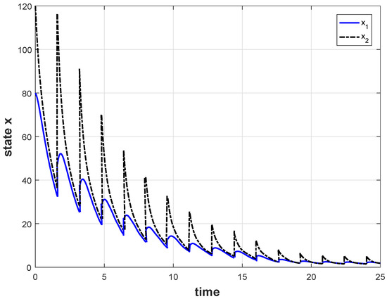
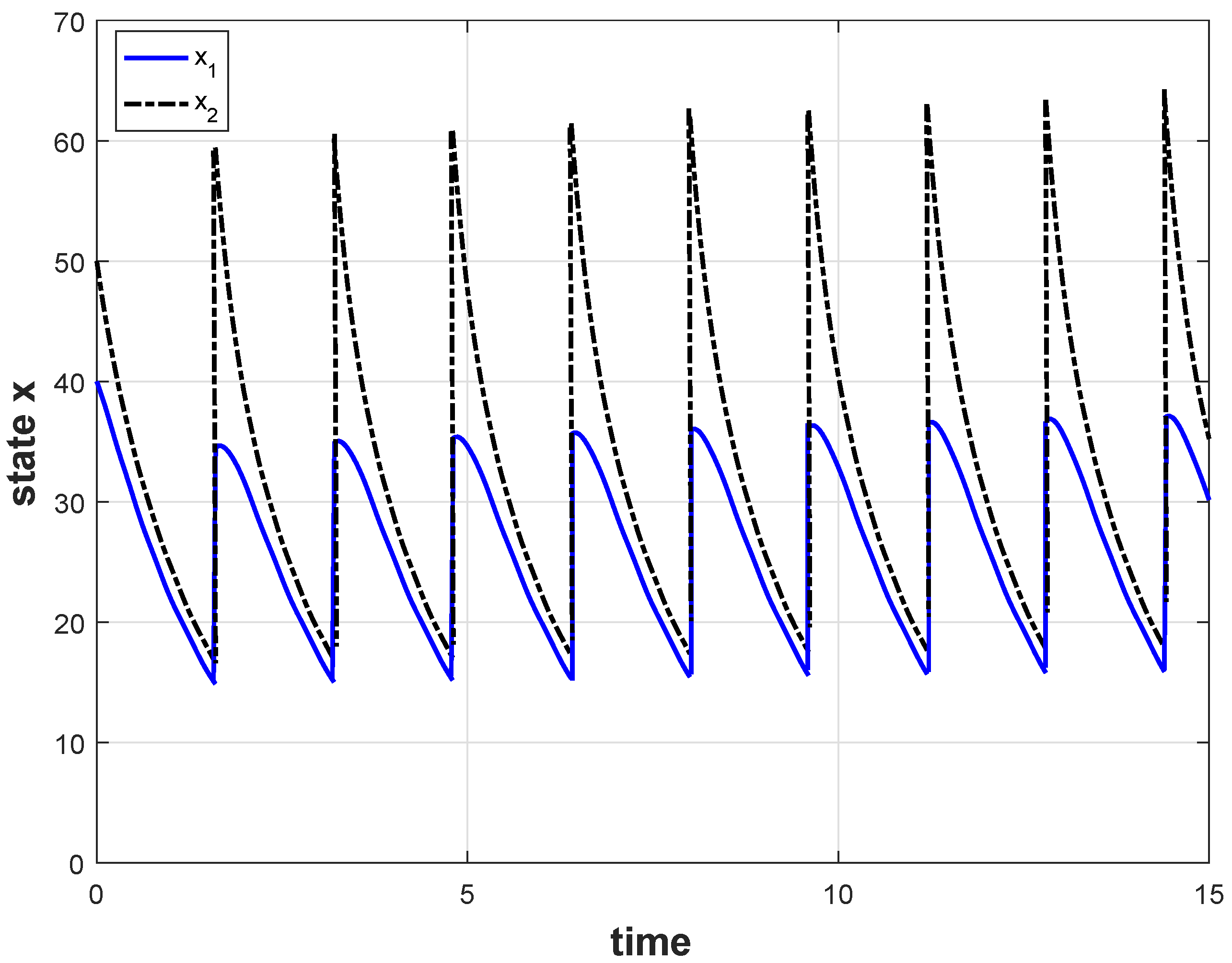
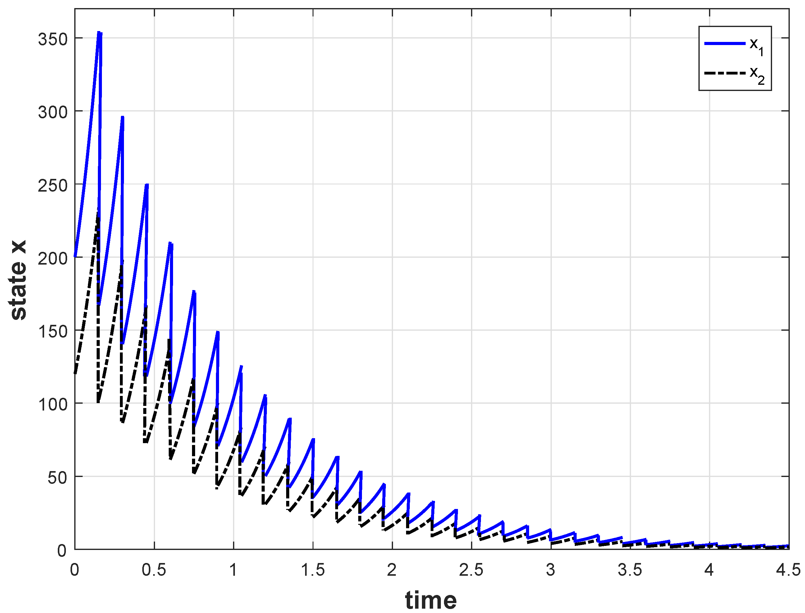
where $\mathsf{\Gamma }=\left[\begin{array}{c}1.21\\ 1.22.5\end{array}\right]$, w is the disturbance input bounded by 1. It is easy to verify that f is cooperative and homogeneous of degree 1; g is continuous on ${\mathbb{R}}_{+}^n$ and bounded by 1; h is non-negative, order-preserving, and homogeneous of degree 1. For system (26), when $w\equiv 1$ and $u\equiv 0$, the simulation curves of ${(x_1,x_2)}^T$ with initial value ${(40,50)}^T$ are shown in Figure 1. Figure 1 shows that the state is ultimately unbounded.

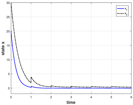
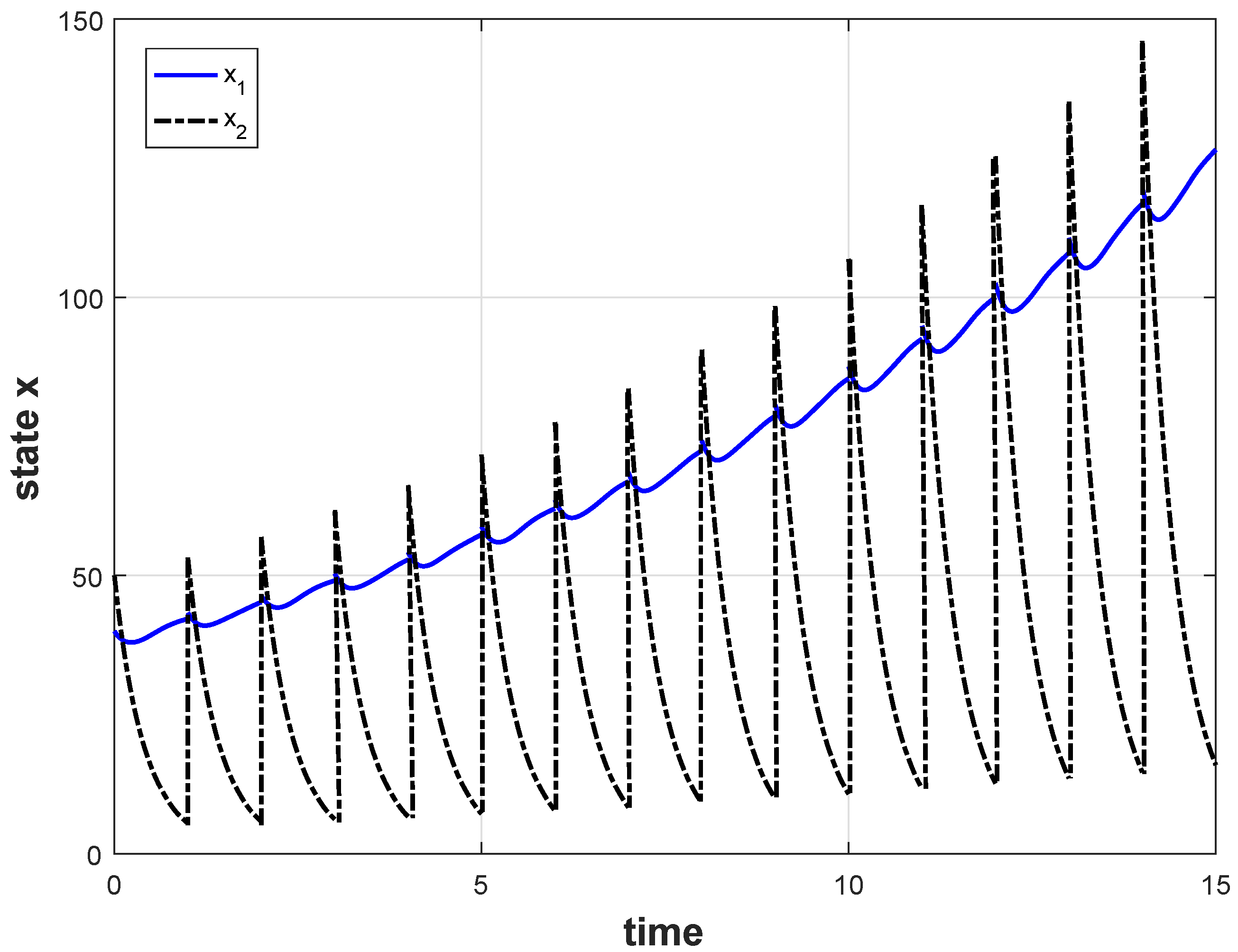
Now, we design an impulsive controller to make system (26) input-to-state stabilizable. We take the impulsive controller in the form of (21) with $K=\frac{1}{{\tilde{v}}^T{B}^{T}v}\tilde{v}{z}^T$. Then, applying the ga function in MATLAB when $T_a=1.6$, $\tilde{v}=\left[\begin{array}{c}1\\ 1\end{array}\right]$ and $\eta =\left[\begin{array}{c}2.7183\\ 2.7183\end{array}\right]$, one feasible solution to Theorem 5 can be obtained:

$$v=\left[\begin{array}{c}0.1437\\ 0.3068\end{array}\right]\mathrm{and}z=\left[\begin{array}{c}-0.2206\\ -0.0004\end{array}\right].$$

Therefore, the impulsive control gain matrix can be obtained. $K=\left[\begin{array}{c}-0.4110-0.0007\\ -0.4110-0.0007\end{array}\right]$. The simulation curves of ${(x_1,x_2)}^T$ with initial value ${(80,120)}^T$ for closed-loop system (30) are shown in Figure 2, which shows that the state ultimately remains bounded.

Example 2.

Consider the nonlinear dynamical system given by (26) with the following:

$$f(x)=\left[\begin{array}{c}3x_1+x_2-3\sqrt{x_1^2+x_2^2}\\ x_1-2x_2-\sqrt{x_1^2+x_2^2}\end{array}\right],g(x)=\left[\begin{array}{c}sin(x_1)\\ cos(x_2)\end{array}\right]\mathrm{and}B=\left[\begin{array}{c}35\\ 0.50\end{array}\right],$$

subject to the following impulses:

$$h(x(t_k))=\mathsf{\Gamma }x(t_k^{-}),$$

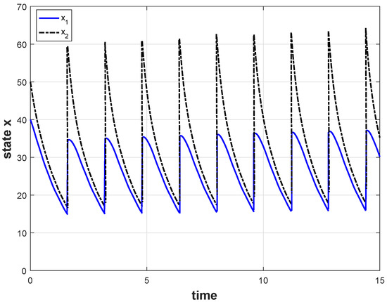
where $\mathsf{\Gamma }=\left[\begin{array}{c}10.2\\ 12\end{array}\right]$, w is the disturbance input bounded by 1. It is easy to verify that f is cooperative and homogeneous of degree 1. g is continuous on ${\mathbb{R}}_{+}^n$ and bounded by 1. h is non-negative, order-preserving, and homogeneous of degree 1. For system (26), when $w\equiv 1$ and $u\equiv 0$, the simulation curves of ${(x_1,x_2)}^T$ with initial value ${(40,50)}^T$ are shown in Figure 3. Figure 3 shows that the state is ultimately unbounded.

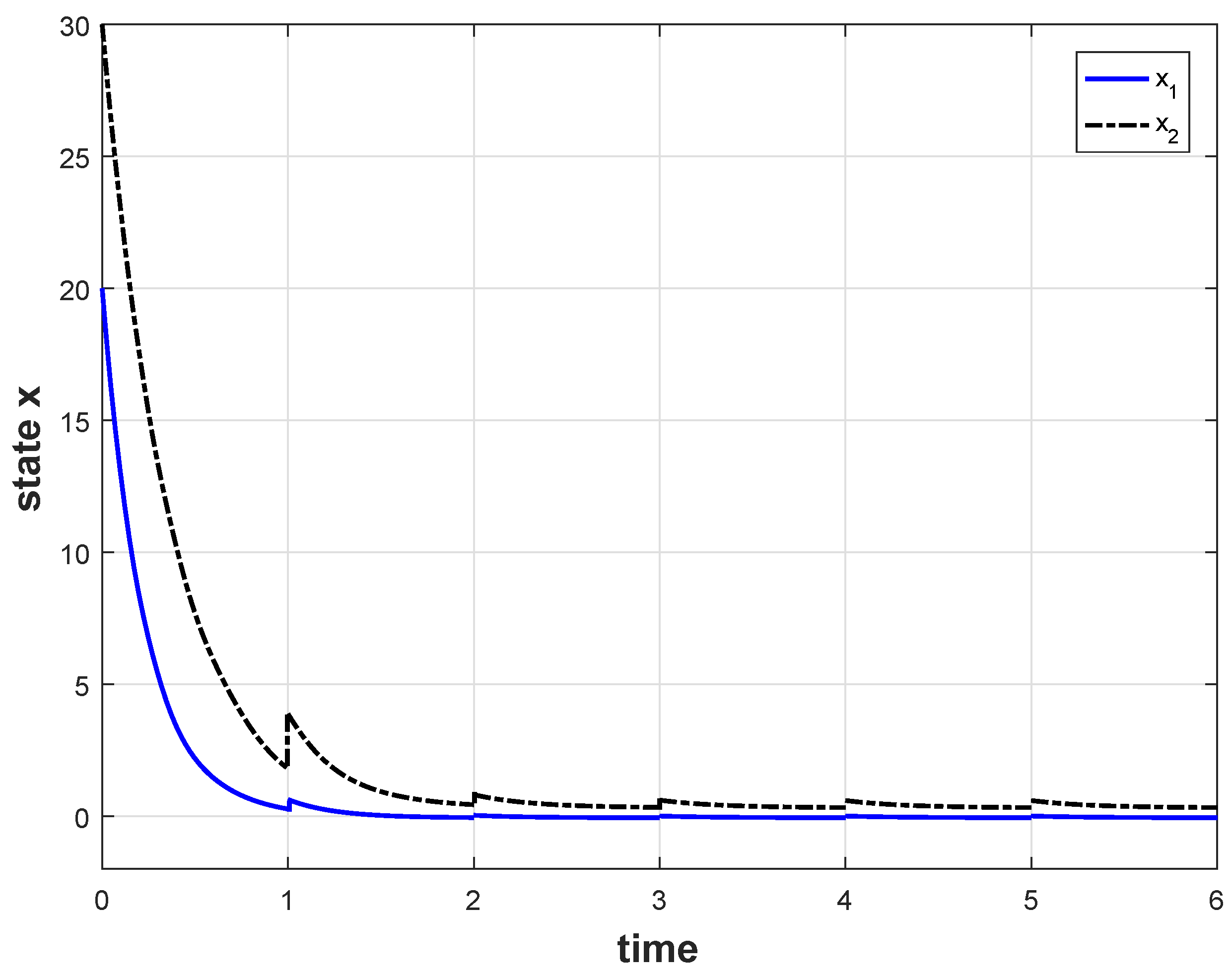
Now, we design a state-feedback controller to make system (26) input-to-state stabilizable. We take the state controller in the form of (16) with $K=\frac{1}{{\tilde{v}}^T{B}^{T}v}\tilde{v}{z}^T$. Then, applying the ga function in MATLAB when $T_a=1$, $\tilde{v}=\left[\begin{array}{c}1\\ 1\end{array}\right]$ and $\eta =\left[\begin{array}{c}4\\ 4\end{array}\right]$, one feasible solution to Theorem 4 can be obtained:

$$v=\left[\begin{array}{c}0.6319\\ 1.0324\end{array}\right]\mathrm{and}z=\left[\begin{array}{c}-4.1649\\ 1.1533\end{array}\right].$$

Therefore, the state control-gain matrix can be obtained. $K=\left[\begin{array}{c}-0.74750.207\\ -0.74750.207\end{array}\right]$. The simulation curves of ${(x_1,x_2)}^T$ for it with initial value ${(20,30)}^T$ are shown in Figure 4. Figure 4 shows that the state remains bounded.

Example 3.

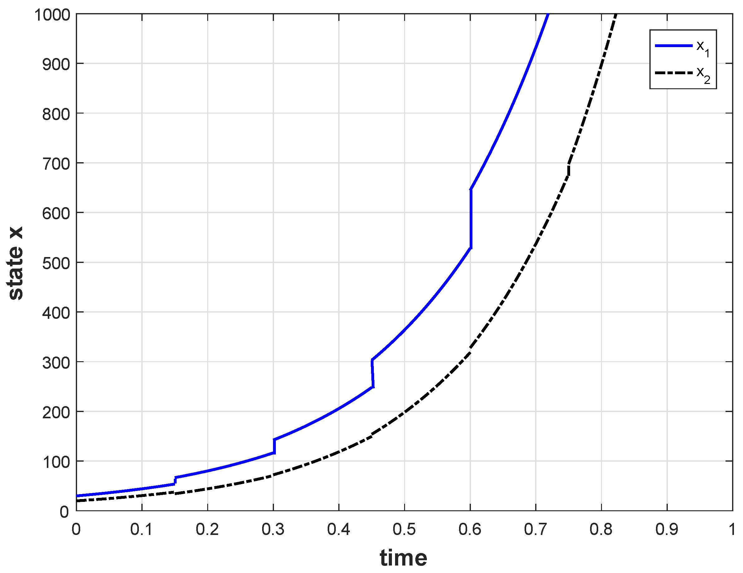
Consider the nonlinear dynamical system given by (26) with the following:

$$f(x)=\left[\begin{array}{c}2x_1+x_2+\sqrt{x_1^2+x_2^2}\\ x_1+x_2+\sqrt{x_1^2+x_2^2}\end{array}\right],g(x)=\left[\begin{array}{c}sin(x_1)\\ cos(x_2)\end{array}\right]\mathrm{and}B=\left[\begin{array}{c}11\\ 0.50.4\end{array}\right],$$

subject to the following impulses:

$$h(x(t_k))=\mathsf{\Gamma }x(t_k^{-}),$$

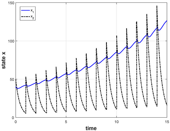
where $\mathsf{\Gamma }=\left[\begin{array}{c}1.10.2\\ 0.50.2\end{array}\right]$, w is the disturbance input bounded by 1. It is easy to verify that f is cooperative and homogeneous of degree 1. g is continuous on ${\mathbb{R}}_{+}^n$ and bounded by 1. h is non-negative, order-preserving, and homogeneous of degree 1. For system (26) with $w\equiv 1$ and $u\equiv 0$, the simulation curves of ${(x_1,x_2)}^T$ with initial value ${(30,20)}^T$ are shown in Figure 5. Figure 5 shows that the state is ultimately unbounded.

Now, we design an impulsive controller to make system (26) input-to-state stabilizable. We take the impulsive controller in the form of (21) with $K=\frac{1}{{\tilde{v}}^T{B}^{T}v}\tilde{v}{z}^T$. Then, applying the ga function in MATLAB when $T_a=0.15$, $\tilde{v}=\left[\begin{array}{c}1\\ 1\end{array}\right]$ and $\eta =\left[\begin{array}{c}0.3\\ 0.3\end{array}\right]$, one feasible solution to Theorem 5 can be obtained:

$$v=\left[\begin{array}{c}1.8135\\ 1.5727\end{array}\right]\mathrm{and}z=\left[\begin{array}{c}-2.1381\\ 0.3307\end{array}\right].$$

Therefore, the impulsive control gain matrix can be obtained. $K=\left[\begin{array}{c}-0.4240-0.0656\\ -0.4240-0.0656\end{array}\right]$. The simulation curves of ${(x_1,x_2)}^T$ for that with initial value ${(200,120)}^T$ are shown in Figure 6. Figure 6 shows that the state remains bounded.

Remark 8.

In Example 1, the continuous dynamics of the system are stable, but the impulsive effects are unstable. Figure 1 shows that the system is ultimately unbounded. Under the effect of the impulsive controller, Figure 2 shows that the system state remains bounded. In Example 2, the continuous dynamics and the impulsive effects of the system are all unstable. Figure 3 shows that the original impulsive positive system is ultimately unbounded. With our state-feedback controller, the continuous dynamics of the system is stable such that the whole impulsive system is stable. Figure 4 verifies it in the aspect of simulation. In Example 3, the continuous dynamics and the impulsive effects of the system are all unstable. This can be verified from Figure 5. In order to stabilize the system, an impulsive controller was designed. Figure 6 shows that the states of the original system with impulsive controller remain bounded.

6. Conclusions

In this paper, the problem of ISS for NIPS was put forward for the first time. On the basis of the max-separable ISS Lyapunov function method, we introduced a sufficient condition on ISS for general NIPS. With regard to the NIPS, the following two cases were included: the continuous dynamics were stable, but the impulsive effects were unstable; the impulses were stable, while the continuous dynamics were unstable. Then, ISS criteria of LTPS and ANIPS were given, respectively. Through them, the ISS properties of the systems were judged directly from the algebraic and differential characteristics of the systems. The ISS criteria were also used for the input-to-state stabilization of LIPS and ANIPS with two kinds of controllers designed: state-feedback and impulsive controllers. Three numerical examples were given to verify the effectiveness of our proposed results.

References

- Farina, L.; Rinaldi, S. Positive Linear Systems: Theory and Applications; Wiley Interscience: New York, NY, USA, 2000. [Google Scholar]
- Benzaouia, A.; Hmamed, A.; Tadeo, F. Stabilisation of controlled positive delayed continuous-time systems. Int. J. Syst. Sci. 2010, 41, 1473–1479. [Google Scholar] [CrossRef]
- Rami, M.A.; Tadeo, F.; Helmke, U. Positive observers for linear positive systems, and their implications. Int. J. Control 2011, 84, 716–725. [Google Scholar] [CrossRef]
- Feng, J.; Lam, J.; Li, P.; Shu, Z. Decay rate constrained stabilization of positive systems using static output feedback. Int. J. Robust Nonlinear Control 2011, 21, 44–54. [Google Scholar] [CrossRef]
- Li, P.; Lam, J. Positive state-bounding observer for positive interval continuous-time systems with time delay. Int. J. Robust Nonlinear Control 2010, 22, 1244–1257. [Google Scholar] [CrossRef]
- Zhao, X.; Zhang, L.; Shi, P. Stability of a class of switched positive linear time-delay systems. Int. J. Robust Nonlinear Control 2013, 23, 578–589. [Google Scholar] [CrossRef]
- Luenberger, D. Introduction to Dynamic Systems; Wiley: New York, NY, USA, 1979. [Google Scholar]
- Kaczorek, T. Stability of fractional positive nonlinear systems. Arch. Control Sci. 2015, 25, 491–496. [Google Scholar] [CrossRef]
- Xiang, M.; Xiang, Z.R. Observer design of switched positive systems with time-varying delays. Circuits Syst. Signal Process. 2013, 32, 2171–2184. [Google Scholar] [CrossRef]
- Nascimento, F.T.; Cunha, J.P.V.S. Positive filter synthesis for sliding-mode control. IET Control Theory Appl. 2019, 13, 1006–1014. [Google Scholar] [CrossRef]
- Wang, J.; Zhao, J. Stabilisation of switched positive systems with actuator saturation. IET Control Theory Appl. 2016, 10, 717–723. [Google Scholar] [CrossRef]
- Zhang, J.S. Stability Analysis of Impulsive Positive Systems; World Congress: Cape Town, South Africa, 2014. [Google Scholar]
- Briat, C. Dwell-time stability and stabilization conditions for linear positive impulsive and switched systems. Nonlinear Anal. Hybrid Syst. 2017, 24, 198–226. [Google Scholar] [CrossRef] [Green Version]
- Sontag, E.D. Smooth stabilization implies coprime factorization. IEEE Trans. Autom. Control 1989, 34, 435–443. [Google Scholar] [CrossRef] [Green Version]
- Sontag, E.D. Comments on integral variants of ISS. Syst. Control Lett. 1998, 34, 93–100. [Google Scholar] [CrossRef]
- Sontag, E.D.; Wang, Y. On characterizations of the input-to-state stability property. Syst. Control Lett. 1995, 24, 351–359. [Google Scholar] [CrossRef]
- Hong, Y.; Jiang, Z.; Feng, G. Finite-time input-to-state stability and applications to finite-time control design. SIAM J. Control Optim. 2010, 48, 4395–4418. [Google Scholar] [CrossRef]
- Zhao, P.; Feng, W.; Kang, Y. Stochastic input-to-state stability of switched stochastic nonlinear systems. Automatica 2012, 48, 2569–2576. [Google Scholar] [CrossRef]
- Sontag, E.D. Input to state stability: Basic concepts and results. Lect. Notes Math. 2008, 12, 163–220. [Google Scholar]
- Jiang, Z.P.; Wang, Y. Input-to-state stability for discrete-time nonlinear systems. Automatica 2001, 37, 857–869. [Google Scholar] [CrossRef]
- Feng, W.; Zhang, J.F. Input-to-state stability of switched nonlinear systems. Sci. China 2008, 51, 1992–2004. [Google Scholar] [CrossRef]
- Huang, L.; Mao, X. On input-to-state stability of stochastic retarded systems with Markovian switching. IEEE Trans. Autom. Control 2009, 54, 1898–1902. [Google Scholar] [CrossRef] [Green Version]
- Teel, A.R.; Nesic, D.; Kokotovic, R.V. A note on input-to-state stability of sampled-data nonlinear systems. Proc. IEEE Conf. Decis. Control 1998, 3, 2473–2478. [Google Scholar]
- Nesic, D.; Teel, A.R. A note on input-to-state stability of networked control systems. Proc. IEEE Conf. Decis. Control 2004, 5, 4613–4618. [Google Scholar]
- Hespanha, J.P.; Liberzon, D.; Teel, A.R. On input-to-state stability of impulsive systems. In Proceedings of the 44th IEEE Conference on Decision and Control, and the European Control Conference 2005 Seville, Seville, Spain, 12–15 December 2005; pp. 3992–3997. [Google Scholar]
- Li, X.; Zhang, X.; Song, S. Effect of delayed impulses on input-to-state stability of nonlinear systems. Automatica 2017, 76, 378–382. [Google Scholar] [CrossRef]
- Dashkovskiy, S.; Mironchenko, A. Input-to-state stability of nonlinear impulsive systems. SIAM J. Control Optim. 2013, 51, 1962–1987. [Google Scholar] [CrossRef] [Green Version]
- Zhao, Y.; Meng, F. Input-to-state stability of nonlinear positive systems. Int. J. Control Autom. Syst. 2019, 17, 3058–3068. [Google Scholar] [CrossRef]
- Jiang, Z.P.; Mareels, I. Input-to-state stabilization on of nonlinear systems with inaccessible state. In Proceedings of the 35th IEEE Conference on Decision and Control, Kobe, Japan, 11–13 December 1996; pp. 4765–4766. [Google Scholar]
- Krstic, M.; Li, Z.H. Inverse optimal design of input-to-state stabilizing nonlinear controllers. IEEE Trans. Autom. Control 1998, 43, 336–350. [Google Scholar] [CrossRef] [Green Version]
- Xie, W.; Wen, C.; Li, Z. Input-to-state stabilization of switched nonlinear system. IEEE Trans. Autom. Control 2001, 46, 1111–1116. [Google Scholar]
- Lu, J.; Ho, D.W.; Cao, J. A unified synchronization criterion for impulsive dynamical networks. Automatic 2010, 46, 1215–1221. [Google Scholar] [CrossRef]
- Angeli, D.; Sontag, E.D. Monotone control systems. IEEE Trans. Autom. Control 2003, 10, 1684–1698. [Google Scholar] [CrossRef] [Green Version]
- Mason, O.; Verwoerd, M. Observations on the stability properties of cooperative systems. Syst. Control Lett. 2009, 58, 461–467. [Google Scholar] [CrossRef] [Green Version]
- Khalil, H.K. Nonlinear Systems, 3rd ed.; Prentice Hall, Inc.: East Lansing, MI, USA, 2002; Volume 38, pp. 1091–1093. [Google Scholar]
- Feyzmahdavian, H.R.; Charalambous, T.; Johansson, M. Exponential stability of homogeneous positive systems of degree one with time-varying delays. IEEE Trans. Automat. Control 2014, 59, 1594–1599. [Google Scholar] [CrossRef] [Green Version]
- Bhatia, R. Matrix Analysis; Springer: Berlin, Germany, 1996. [Google Scholar]
Publisher’s Note: MDPI stays neutral with regard to jurisdictional claims in published maps and institutional affiliations. |
© 2021 by the authors. Licensee MDPI, Basel, Switzerland. This article is an open access article distributed under the terms and conditions of the Creative Commons Attribution (CC BY) license (https://creativecommons.org/licenses/by/4.0/).