Uncertain Interval Forecasting for Combined Electricity-Heat-Cooling-Gas Loads in the Integrated Energy System Based on Multi-Task Learning and Multi-Kernel Extreme Learning Machine

Abstract

The accurate prediction of electricity-heat-cooling-gas loads on the demand side in the integrated energy system (IES) can provide significant reference for multiple energy planning and stable operation of the IES. This paper combines the multi-task learning (MTL) method, the Bootstrap method, the improved Salp Swarm Algorithm (ISSA) and the multi-kernel extreme learning machine (MKELM) method to establish the uncertain interval prediction model of electricity-heat-cooling-gas loads. The ISSA introduces the dynamic inertia weight and chaotic local searching mechanism into the basic SSA to improve the searching speed and avoid falling into local optimum. The MKELM model is established by combining the RBF kernel function and the Poly kernel function to integrate the superior learning ability and generalization ability of the two functions. Based on the established model, weather, calendar information, social–economic factors, and historical load are selected as the input variables. Through empirical analysis and comparison discussion, we can obtain: (1) the prediction results of workday are better than those on holiday. (2) The Bootstrap-ISSA-MKELM based on the MTL method has superior performance than that based on the STL method. (3) Through comparing discussion, we discover the established uncertain interval prediction model has the superior performance in combined electricity-heat-cooling-gas loads prediction.

1. Introduction

With the rapid development of China’s economy and the rapid growth of energy demand, energy development is facing great challenges from resources and the environment. It is a new direction of energy development and reform to construct a clean, low-carbon, safe, and highly efficient energy system to maximize the development and utilization of renewable energy and to improve the efficiency of energy utilization. In this context, the integrated energy system (IES) has become an important direction of the future transformation of China’s energy system. The development of the IES with multi-energy and mutual aid centered on electric energy is conducive to further improving the energy efficiency of users and optimizing the energy structure. The accurate forecasting of renewable energy generation on the supply side and multi-energy loads on the demand side is the foundation of the construction and stable operation of the IES.

1.1. Research Motivation

With the exploitation and utilization of renewable energy and the rapid development of economy and society, the form of energy supply and demand in China has become more diversity [1]. Simultaneously, there are problems such as decentralized planning, independent operation, and separated management of energy supply and demand network. Hence, it is urgent to innovate new modes of energy supply and demand. In this context, multi-energy complementary integration optimization has become the breakthrough and the significant direction of China’s energy transformation and revolution in the future [2]. With the collaborative and efficient utilization of the traditional fossil energy power generation and the emerging distributed energy power generation, the integrated energy system for the electricity, heat, cooling, gas, and other energy demands of the end-users has become a critical part of multi-energy complementary integration optimization and an important subset of energy internet. The IES has the advantages of highly efficient consumption of renewable energy, coordinated utilization of multi-energy, and flexible operation modes, therefore, it has been widely considered and vigorously developed by many countries all over the world [3].

However, there are some uncertainties existing in the IESs, which mainly originate from the supply side uncertainties of distributed renewable energy power generation including wind power generation, photovoltaic power generation, etc., and the demand side uncertainties of electricity, heating, cooling, gas and other demands. As the sources of supply side and demand side uncertainty factors in the IES are gradually various, the degree of uncertainty is increasing, and the characteristics of uncertainty are becoming increasingly complicated, the accurate prediction of energy supply and demand can provide important references and decision-making basis for multi-energy planning and optimal scheduling, demand side management, as well as safe and stable operation of the IESs [4]. Previous literature mainly focused on researching the uncertainty prediction of renewable energy power generation, but rarely investigated the uncertainty prediction of multi-energy loads on the demand side. Load prediction on the demand side is the precondition and foundation to ensure reliable and economic operation for the IESs. As early as 1985, an investigation [5] in Britain illustrated that the annual economic loss would be 10 million pounds as the error of power load prediction increased one percentage. It was also shown in Reference [6] that when the forecasting error was reduced by 1%, 58,780 MW of energy consumption can be saved in a year. Therefore, under the background of the rapid development of the IESs, load prediction on the demand side with high accuracy plays a significant role in improving energy management and dispatching in the IESs.

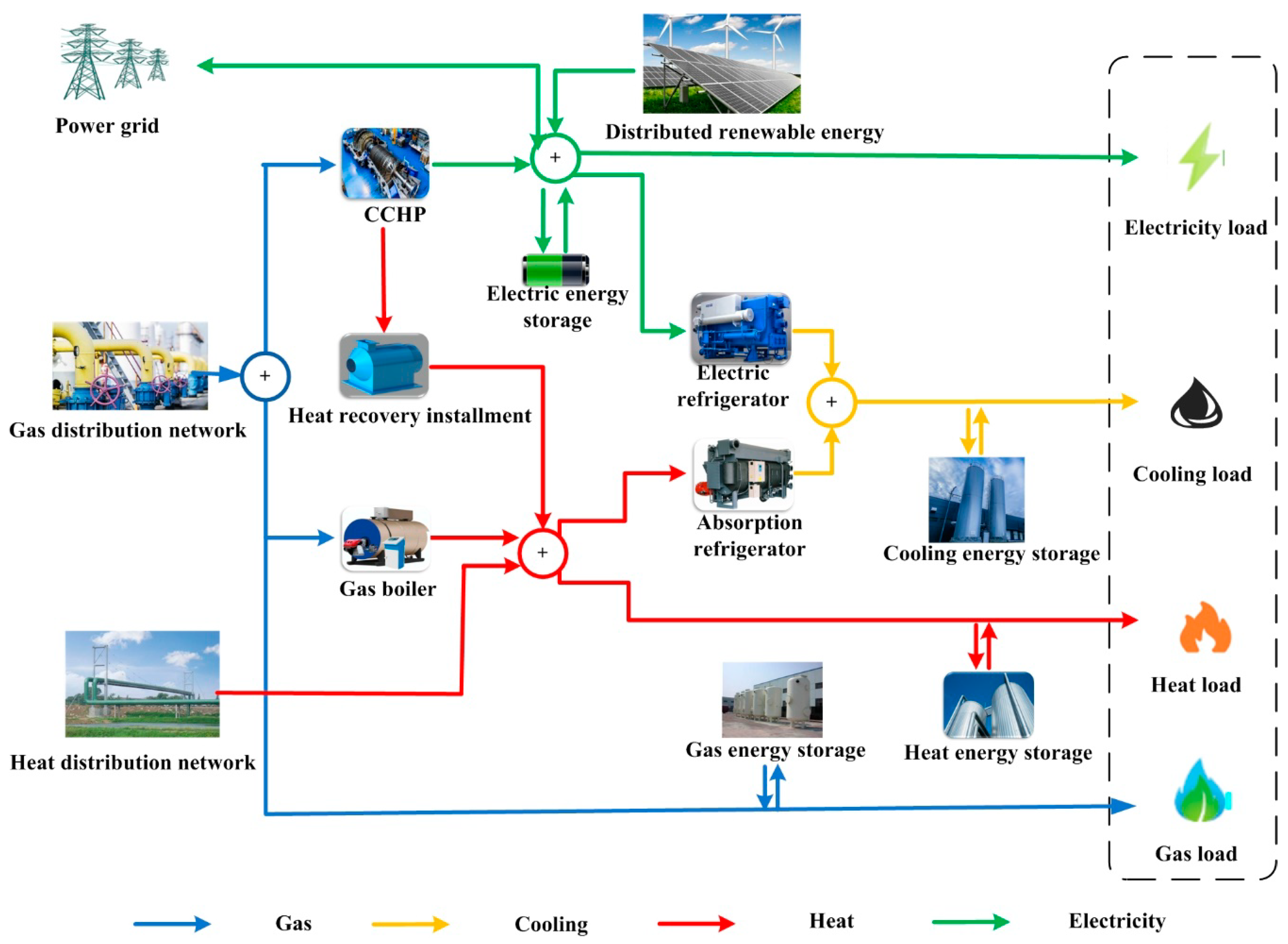
1.2. The Analysis of the Complicated Coupling Relations among the Various Energy Subsystems in the IES

The IES aims to improve energy utilization efficiency and reduce pollutant emissions. Through the mutual conversion of electric, natural gas, heat and cooling energy, the IES can couple the power grid, natural gas distribution network as well as heat distribution network in a certain region, so as to realize the conversion and utilization, complementary coupling, and collaborative optimization of different energy sources [7]. The energy production, conversion, storage, and consumption process are illustrated in Figure 1. As can be seen from Figure 1, on the basis of the IES operation characteristics and energy conversion process, the IES can satisfy the demand of electricity, heat, cooling, and gas loads. The IES is made up by the electric energy subsystem, cooling energy subsystem, heat energy subsystem, and gas energy subsystem.

For the electric energy subsystem, it is the most significant subsystem in the IES, interacting with other energy subsystems frequently. The electric energy mainly originates from distributed renewable energy generating units, the electric power network, combined cooling-heat-power (CCHP) units, and energy storage batteries, etc. The consumption of electric energy primarily includes energy storage batteries, electric hydrogen generation system, electric boiler and heat pump, electric refrigerator, electric vehicle charging pile, users electric load, etc. The coupling and transformation between electric energy and other energy sources contain converting electric energy into gas energy through power to gas (P2G) converter, converting electric energy to heat energy through electric heating boiler and heat pump, and converting electric energy to cooling energy through electric refrigerator.

For the heat energy subsystem, the heat energy primarily originates from the exterior heating network, heat storage tank, CCHP units, combined heat and power (CHP) units, electric boiler, heat pump, etc. The consumption of heat energy primarily contains users heat load, absorption refrigerator, heat storage tank, etc. The heat energy subsystem can generate electricity employing waste heat energy produced by the CCHP units and distribute the electricity to the electric energy subsystem. The heat energy subsystem can also use the gas energy generated by the CCHP units to produce electricity and heat energy to satisfy the heat demand.

For the cooling energy subsystem, the cooling energy mainly comes from the CCHP units, cooling energy storage equipment, electric refrigerator, absorption refrigerator, etc. The consumption of cooling energy includes air conditioning, refrigerators, and other refrigeration equipment. Generally, the cooling energy subsystem generates cooling energy through the electric refrigerator employing the electric energy generated by the electric energy subsystem. It can also use the heat energy from the CCHP units to generate cooling energy through the absorption refrigerator.

For the gas energy subsystem, the source of gas energy mainly includes an exterior gas distribution network, electric hydrogen generation system, gas storage tank, etc. The consumption of gas mainly contains CHP units, CCHP units, a gas storage tank, gas filling station, and users’ gas load. The coupling and conversion between gas energy and other energy sources includes converting gas energy into electric energy, heat energy and cooling energy through CHP units and CCHP units. The gas storage tank maintains the balance between the supply and demand of gas by charging and discharging gas energy.

As previous description, there exist strong coupling relations among the electric energy subsystem, the heat energy subsystem, the cooling energy subsystem, and the gas energy subsystem, which makes the IES coordinated operation to a maximum degree. Therefore, in order to predict the combined electricity-heat-cooling-gas loads on the demand side of the IES accurately, the complicated coupling relations are need to be taken into account.

1.3. Literature Review

Two factors need to be considered when predicting the combined loads on the demand side of the IES. One is the selection of input variables for the combined load prediction model, and the other is the methods employed to forecast the combined load. As is shown in previous literature, the input variables selected for load forecasting model of a single energy type are greatly different. For example, in terms of the electricity load prediction, historical load data, weather condition, calendar information, and electricity price are considered by Yang et al. [8] to propose a probability density prediction methodology to forecast the electric power load on the basis of the quantile regression of the Gauss process. Guo et al. [9] established a probability density prediction approach based on deep learning mechanism taking atmospheric pollutants factors (e.g., CO, SO2, PM2,5, etc.), date related factors (e.g., seasonal, monthly, daily data), weather related factors (e.g., daily temperatures, rainfall amount, etc.), and economic factors (e.g., economic structure influencing residential living standards) into account to predict electricity consumption. Kim et al. [10] took the weather and holiday related variables as the critical factors to predict peak load demand. Recently, a few studies employed feature selection methods to select the informative input variables for load forecasting model to improve the prediction accuracy. For example, autocorrelation function is employed by Yang et al. [11] to select the optimal input feature to improve the half-hour electricity load prediction accuracy. In terms of the heat load prediction, the weather condition and historical load data are considered by Geysen et al. [12]. Suryanarayana et al. [13] selected the last 7 days of heat load and the next 24 h temperature prediction results as the heat load forecasting input variables. Nigitz et al. [14] considered the ambient temperature for each hour of the day as the critical influencing factor of heat load forecasting. In terms of the cooling load prediction, Zhou et al. [15] considered the historical load data and weather conditions as the input variables for cooling load prediction. Ahmad et al. [16] considered climate related factors as the input variables for the cooling load prediction model. In terms of the gas load prediction, temperature, seasonal index, price of natural gas and oil, exchange rate, as well as the population and gross domestic product (GDP) of the Istanbul province are considered by Beyca et al. [17] to input into the established gas consumption prediction model. Additionally, Shi et al. [18], taking the historical load data, weather condition, economic data, and calendar information into account, established a combined electricity-heat-gas load forecasting model. Tan et al. [19] established a combined electricity-heat-cooling-gas load prediction model on the basis of multi-task learning and the least square support vector machine, considering weather-related factors, calendar information, primary economic factors, and technical conditions.

Forecasting techniques employed to load prediction can be classified into two primary categories, including traditional statistical methods and artificial intelligent (AI) based methods. Traditional statistical methods, widely used in load prediction, contain the Auto-Regressive-Integrated-Moving-Average (ARIMA) models [20,21,22,23,24], time series regression models [25,26,27,28], fuzzy models [29,30,31,32], and grey prediction models [33,34,35,36]. AI-based methods are generally adaptive and robust to non-stationary data and make the prediction results with high accuracy. The most widely used AI-based methods include neural network models [37,38,39,40], the least square support vector machine optimized by various intelligent optimization algorithms [41,42,43,44], and extreme learning machine method optimized by various intelligent optimization approaches [45,46,47].

Previous literatures researching on the load forecasting mainly focused on single energy load. However, with the rapid development of computer technology and the construction of the integrated energy systems combined with multi-energy types, the multi-task learning (MTL) method gradually replaces the single task learning (STL) method in the application of load forecasting [48]. It is difficult for the traditional STL method to obtain sufficient information of data distribution through training, which results in ignoring the complicated inter-relation among various factors, and hence decreasing the learning effect [49]. Considering about this, the multi-task learning (MTL) method is proposed, which can exactly explore the inter-relations among different tasks [50,51]. In load forecasting applications, Nunes et al. [52] compared the prediction results obtained by the artificial neural networks (ANN) on the basis of the STL and the MTL methods, and then the comparison results demonstrated that the ANN based on the MTL method has a superior performance than that based on the STL method. Shireen et al. [53] combined the MTL method with time series regression and the results showed that the prediction accuracy has been improved effectively. Tan et al. [19] combined the MTL method with the least square support vector machine to apply in electricity-heat-cooling-gas load forecasting, and through comparing with other models, it can be found that the established model is the most time-saving and can obtain the forecasting results with the highest accuracy. In the IES, energy conversion elements (such as CCHP units, electric boilers, electric refrigerators, energy storage, etc.) are used to realize the coupling of electricity, heat, cooling and gas, which will result in strong coupling relationships existing among electricity, heat, cooling and gas sub-systems. In the IESs, a large amount of energy conversion and sharing information of electricity, heat, cooling, and gas exists in the data, and the characteristics of various energy conversion are complicated. Considering this, the MTL method is employed to establish the electricity-heat-cooling-gas loads forecasting model, which can effectively employ the complicated shared information of various energy conversion in the IES, so as to improve the multi-energy load forecasting accuracy.

The forecasting techniques, including traditional statistical methods and AI-based methods, generally belong to the deterministic prediction model. However, the electricity-heat-cooling-gas load on the demand side in the IES is a complicated dynamic system affected by weather related factors, calendar information, social–economic factors, and technical conditions with nonlinear, high-dimensional, and uncertain characteristics. Considering the various factors influencing the electricity-heat-cooling-gas loads on the demand side in the IES and the errors that exist in the process of statistics and monitoring, there are uncertainties in the prediction of the combined electricity-heat-cooling-gas loads on the demand side in the IES. Contemporarily, the existing researches mainly focused on single points prediction, which cannot characterize the influence of uncertainties on the combined electricity-heat-cooling-gas loads prediction. Therefore, it is necessary to consider the influence of uncertainties when forecasting the combined electricity-heat-cooling-gas loads on the demand side of the IES, and extend the single point prediction to the uncertainty interval prediction, so as to improve the reliability of the prediction results. In recent years, interval prediction theory is a common method to research on the prediction problem with uncertainties. The prediction results are expressed in the form of interval to represent the uncertainty characteristics of the prediction problem. Compared with the single point prediction method, the interval prediction method can obtain the change range of the predicted object in a period of time in the future by means of interval expression, and quantify the reliability of the prediction model according to the interval width and coverage probability, so as to make the prediction results of the model with high reliability [54]. At present, the commonly used interval prediction methods mainly include mean variance estimation method, upper and lower limit estimation method, delta method, Bayesian method and Bootstrap method [55,56,57,58,59,60,61,62]. The Bootstrap method can approximate the sample distribution characteristics without subjective assumption, but only through repeated sampling, and then can effectively construct the prediction interval, which has the advantages of high accuracy and reliability [61]. Therefore, in this paper, the Bootstrap method is used to establish the electricity-heat-cooling-gas load uncertain interval prediction model.

As previous introduction, extreme learning machine (ELM) method optimized by various intelligent optimization approaches is widely applied in load forecasting. ELM method is a kind of machine learning method established based on a feed-forward neuron network, which is suitable for supervised learning and unsupervised learning problems. The connection weights between input layer and hidden layer and the threshold value of hidden layer neurons are generated randomly. In the training process, the only optimal solution can be obtained by setting the number of hidden layer neurons [63,64]. Compared with the traditional Back-Propagation neural network algorithm, the ELM method has fast learning speed and good generalization performance. However, due to the randomness of ELM feature mapping and its sensitivity to noise, the robustness and generalization ability of the ELM method are reduced. Based on this, Kernel Extreme Learning Machine (KELM) is proposed by introducing the kernel method and regularization coefficient into the ELM method, the influence of random mapping and sample noise on the model can be decreased, and the prediction accuracy of the model can be improved [65,66]. However, the KELM method only considers one kernel form in the prediction, which is difficult to apply to the prediction of the combined electricity-heat-cooling-gas load on the demand side of the IES with multiple data characteristic samples. Therefore, it is necessary to use multi-kernel form to establish a multi-energy load forecasting model. Simultaneously, when employing the multi-kernel extreme learning machine (MKELM) model, it is necessary to determine the relevant parameters in the model. The model parameters set by subjective knowledge always lead to low prediction accuracy. Therefore, this paper uses a new bionic intelligent optimization algorithm named Salp Swarm Algorithm (SSA) to optimize the parameters of the MKELM model. In order to improve the convergence performance of SSA and make it better to solve the high-dimensional complex parameters optimization problem in the optimization process, an improved SSA (ISSA) is proposed in this paper, which introduces the dynamic inertia weight and chaotic local searching mechanism into the basic SSA to improve the searching speed and avoid falling into local optimum.

Above all, this paper established an uncertain interval forecasting model for the combined electricity-heat-cooling-gas loads in the IES based on the MTL method, the Bootstrap method, the MKELM method, and the ISSA.

1.4. Our Contributions

Contemporarily, researches on load forecasting of various energy types are relatively mature. With the continuous development of energy reform and energy transformation, the construction of the IES has received great attention, and the accurate prediction of energy on supply and demand sides of the IES is the foundation of the construction of the IES and can ensure the safe and stable operation of the IES. However, it is difficult to find the studies focused on forecasting the combined load based on the coupling relations among integrated energy subsystems. At the aim of filling this gap and exploring the coupling relations deeply, this research establishes a hybrid load prediction model for the IES on the basis of the MTL method, the Bootstrap method, the MKELM, and the ISSA. The contributions of this research are as follows:

(1)

The complicated coupling relations among the various integrated energy subsystems are untangled systematically, and the significant input variables of the established hybrid load prediction model are determined.

(2)

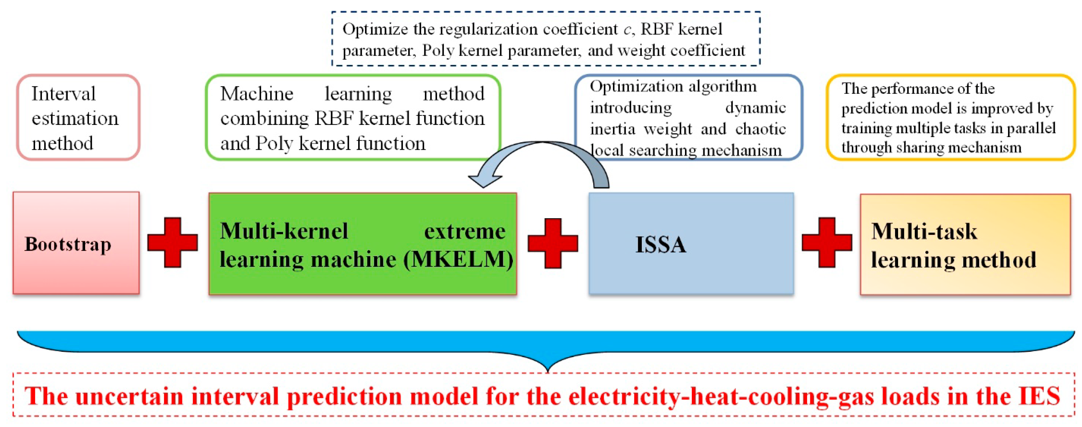
The uncertain interval forecasting model of the combined electricity-heat-cooling-gas loads in the IES is established based on the MTL method, the Bootstrap method, the MKELM, and the ISSA.

(3)

Aiming at solving the problems of local optimum, low convergence speed, and low precision of the basic SSA, the improved SSA (ISSA) is proposed by introducing the inertia weight mechanism and chaotic local searching strategy into the basic SSA.

(4)

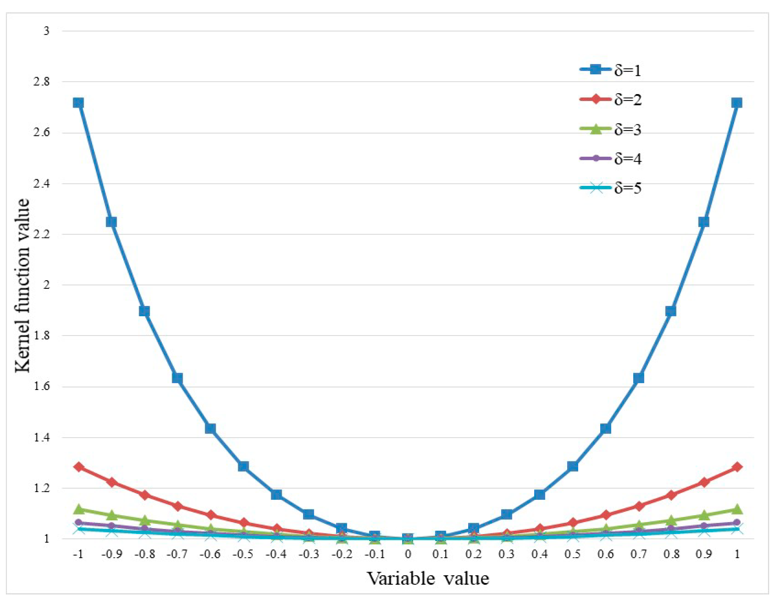
The MKELM model is proposed by combining the RBF kernel function and the Poly kernel function, so as to integrate the superior learning ability and the generalization ability of the two kernel functions.

1.5. Organization of the Research

The rest parts of the research are organized as follows. The methodology of the MTL method, the Bootstrap method, the MKELM, and the ISSA as well as the calculation process of the established uncertain interval forecasting model are introduced in Section 2. The numerical analysis is conducted in Section 3. The comparison discussion on the forecasting results obtained by the MTL method and STL method as well as other optimization algorithms and kernel functions of the ELM are provided in Section 4. Section 5 summarizes the primary conclusions of this research.

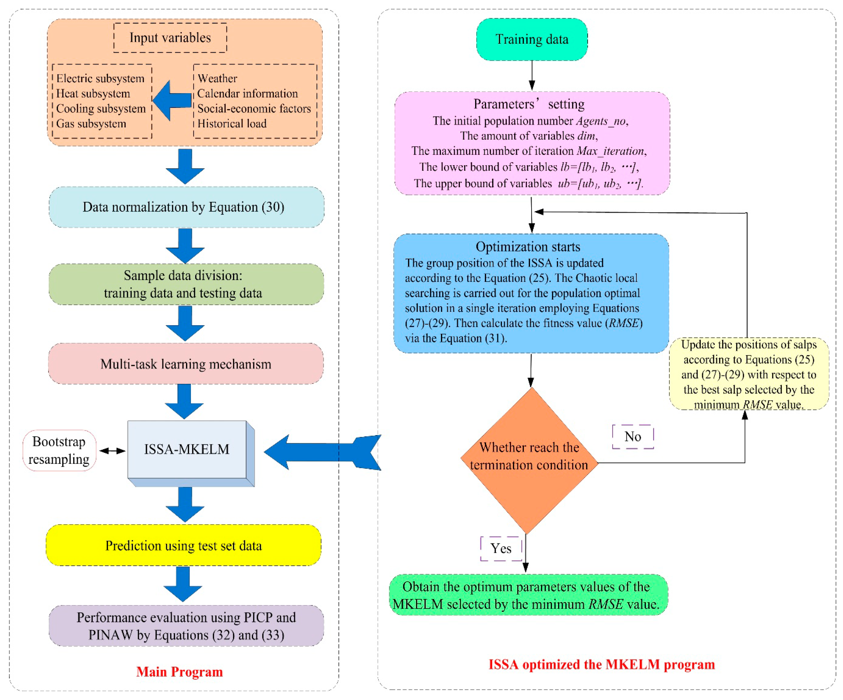
2. Materials and Methods

An uncertain interval forecasting model for the combined electricity-heat -cooling-gas loads on the demand side of the IES is established in this paper based on the MTL method, the Bootstrap method, the MKELM, and the ISSA. The established model is not only a combination of several methods, but also makes great improvement for the MKELM and the original SSA.

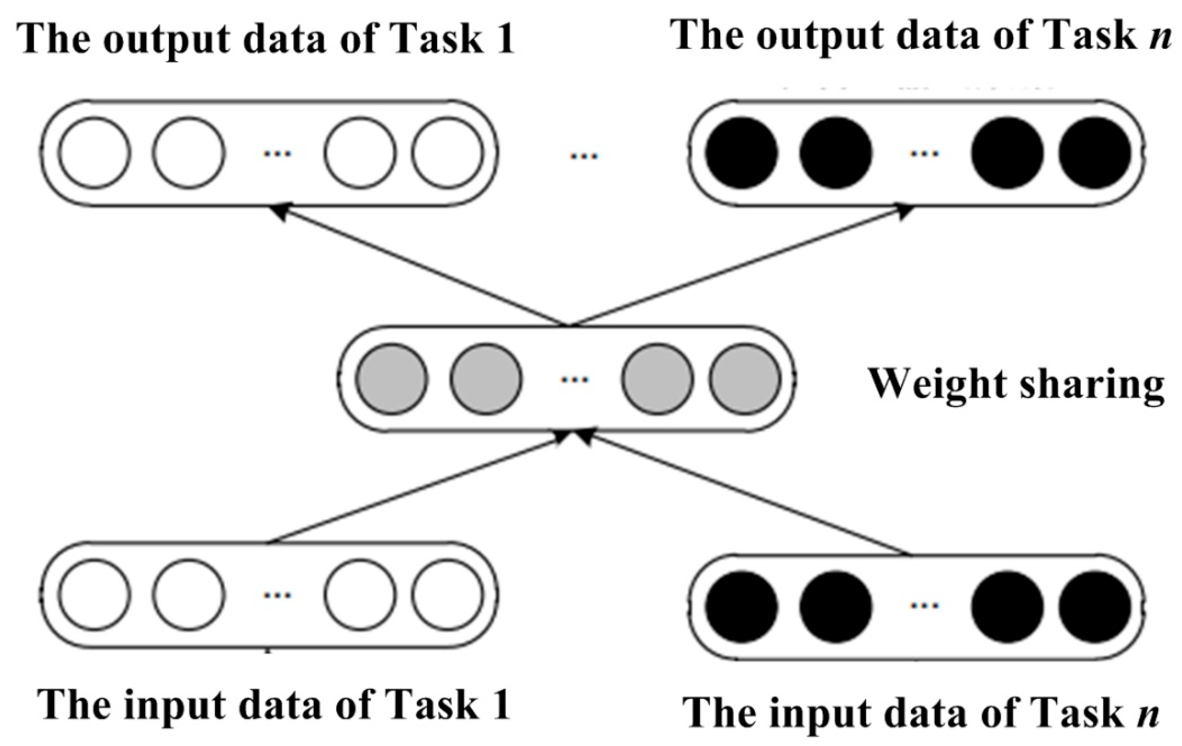
2.1. The Multi-Task Learning Method

The MTL method is a classical inductive transfer mechanism method in the machine learning field. It employs the information hidden in multiple related tasks to improve the generalization ability of algorithms. The MTL method improves the performance of the prediction model by using the sharing mechanism to train multiple tasks in parallel. When studying a problem, it can learn and acquire knowledge of other related problems by using shared information [67]. The information sharing mechanism of the MTL method is shown in Figure 2.

In the IES, various energy subsystems, such as electric energy subsystem, heat energy subsystem, cooling energy subsystem, and gas energy subsystem, are coupled by energy flow through different energy conversion equipment, including CCHP units, electric boiler, gas boiler, electric refrigerator, absorption refrigerator, etc. According to the description in Section 1.2, there exist a strong coupling relation among different energy subsystems. A large amount of energy conversion sharing information exists in the data, which are difficult to be extracted and summarized by traditional manual feature extraction methods. Therefore, the MTL method is combined into the multi-energy load forecasting model, which can effectively employ the complicated sharing information of electricity, heat, cooling, gas, and other energy conversion, help machine learning and bionic intelligent optimization algorithms to train better abstract characteristics, and improve the forecasting precision of multi-energy loads in the IES [19].

Suppose there are T target tasks, and the data of each task originates from the generalized function space $X\times Y,X\in R^n,Y\in R$. Each task contains m training sample sets $\left\{\left(x_{1t},y_{1t}\right),\left(x_{2t},y_{2t}\right),\cdots ,\left(x_{mt},y_{mt}\right)\right\}$. Each task has a sample distribution $P_t$, and each task is different but related.

In the MTL method, the goal of the multi-tasks is to learn $f_1,f_2,\cdots f_T$ [19]

$$f_t\left(x_{it}\right)=y_{it}$$

(1)

where $f_t\left(x_{it}\right)$ is the training function of T tasks, and $y_{it}$ is the training sample.

In order to balance the correlation and constraint among different tasks, it is necessary to consider the learning optimization goals among different tasks to obtain better learning effects [68]. There are differences among tasks, but the association among tasks can be realized by sharing information path.

2.2. The Bootstrap Method

The Bootstrap method is an important statistical method in non-parametric statistics to estimate the variance of statistics and then to evaluate the interval. It is a statistical method based on repeated sampling. The prediction interval established by this method can not only accurately represent the uncertainty degree of the prediction object, but also analyze the change range of the time series of the prediction object in a period of time in the future, which can effectively make up for the limitations of the single point prediction method [69]. In the combined electricity-heat-cooling-gas loads forecasting, considering the characteristics, various uncertainties will affect the forecasting accuracy of the prediction model, while combining the Bootstrap method into the multi-energy load forecasting model to predict the interval of multi-energy load can improve the prediction precision and make the forecasting results better applied to engineering practice.

Supposing the sample of the combined electricity-heat-cooling-gas load prediction is $D={\left\{x_i,t_i\right\}}_{i=1}^N$, $x_i$ is the set of influencing factors affecting the combined electricity-heat-cooling-gas load, $t_i$ is the actual values of the electricity-heat-cooling-gas load, therefore,

$$t_i-f(x_i)=[\overline{f}(x_i)-f(x_i)]+\epsilon (x_i)$$

(2)

where $f(x_i)$ is the forecasting values of the electricity-heat-cooling-gas load, $\overline{f}(x_i)$ is the actual regression values of the electricity-heat-cooling-gas load forecasting model, and $\epsilon (x_i)$ is the data noise [70].

In the Equation (2), $t_i-f(x_i)$ is the total error between the actual value and the forecasting value of the electricity-heat-cooling-gas load, and $\overline{f}(x_i)-f(x_i)$ is the prediction model error of the electricity-heat-cooling-gas load. The total error consists of prediction model error and data noise. Assuming that all errors are unbiased, and then the variables can be estimated according to the variance.

The Bootstrap method can obtain M sub-samples by repeatedly sampling the electricity-heat-cooling-gas load samples, and then train the electricity-heat-cooling-gas load forecasting model, and estimate the model error variance according to Equation (3).

$${\sigma }_{\Delta }^2(x)=\frac{1}{M-1}{\displaystyle \sum _{k=1}^M{(\overline{f}(x)-f_k(x))}^2}$$

(3)

where ${\sigma }_{\Delta }^2(x)$ is the error variance of the forecasting model, representing the model uncertainties caused by human subjective factors such as the structure and the parameters setting of the forecasting model. $\overline{f}(x)$ is the expected values of the output of M prediction models, and $f_k(x)$ is the prediction value of the output of the k-th model.

In the Bootstrap method, the data noise variance represents the uncertainties of the electricity-heat-cooling-gas loads samples caused by random noise, and can be estimated according to Equation (4)

$${\sigma }_{\epsilon }^2(x)=E\left\{{\left[t-f(x)\right]}^2\right\}-{\sigma }_{\Delta }^2(x)$$

(4)

where ${\sigma }_{\epsilon }^2(x)$ is the data noise variance, and E represents the expected value.

At the aim of effectively predicting the data noise variance ${\sigma }_{\epsilon }^2(x)$, we need to construct the square residual sequence of the prediction model, and combine it into a new sample set $D_{new}={\left\{x_i,r_i\right\}}_{i=1}^N$, and then train the prediction model according to the new sample set. Among them, $r_i$ can be obtained through Equation (5).

$$r_i=\max ({(t_i-f(x_i))}^2-{\sigma }_{\Delta }^2(x),0)$$

(5)

When training the new sample set, in order to maximize the probability of noise variance appearing in the electricity-heat-cooling-gas load samples, the maximum likelihood method is used to train the new model, so as to ensure the prediction confidence level. The objective function is

$$C_N=\frac{1}{2}{\displaystyle \sum _{i=1}^N\left[\frac{r_i^2}{{\sigma }_{\epsilon }^2(x)}+\ln ({\sigma }_{\epsilon }^2(x))\right]}$$

(6)

After the training of the forecasting model, the forecasting interval of the electricity-heat-cooling-gas load with significance level $\alpha$ can be constructed as follows:

$$\overline{f}(x)\pm z_{1-\alpha /2}\sqrt{{\sigma }_{\Delta }^2(x)+{\sigma }_{\epsilon }^2(x)}$$

(7)

where $1-\alpha /2$ is the quantile in the standard Gaussian distribution [71].

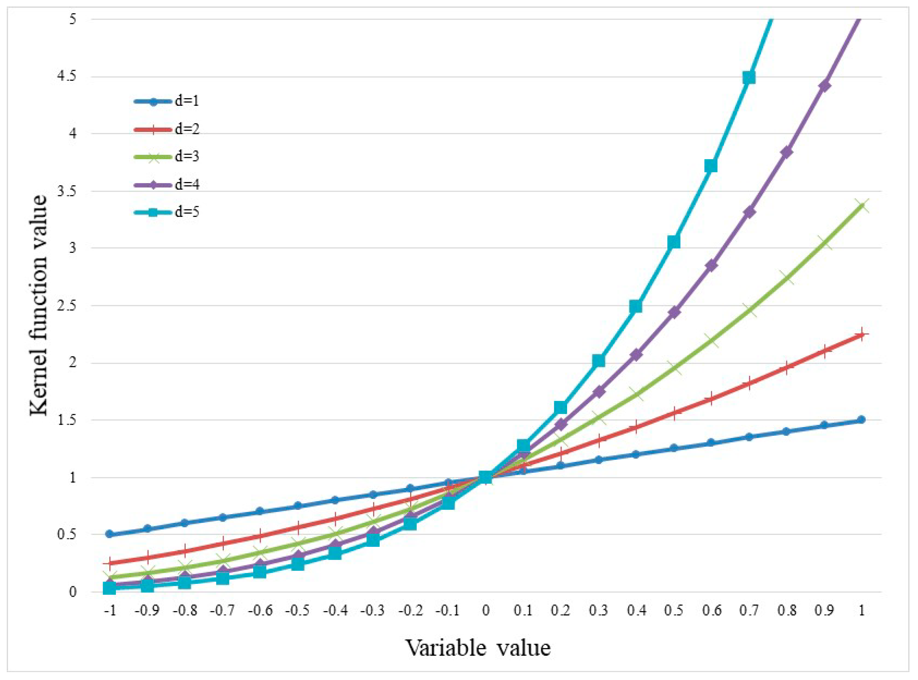
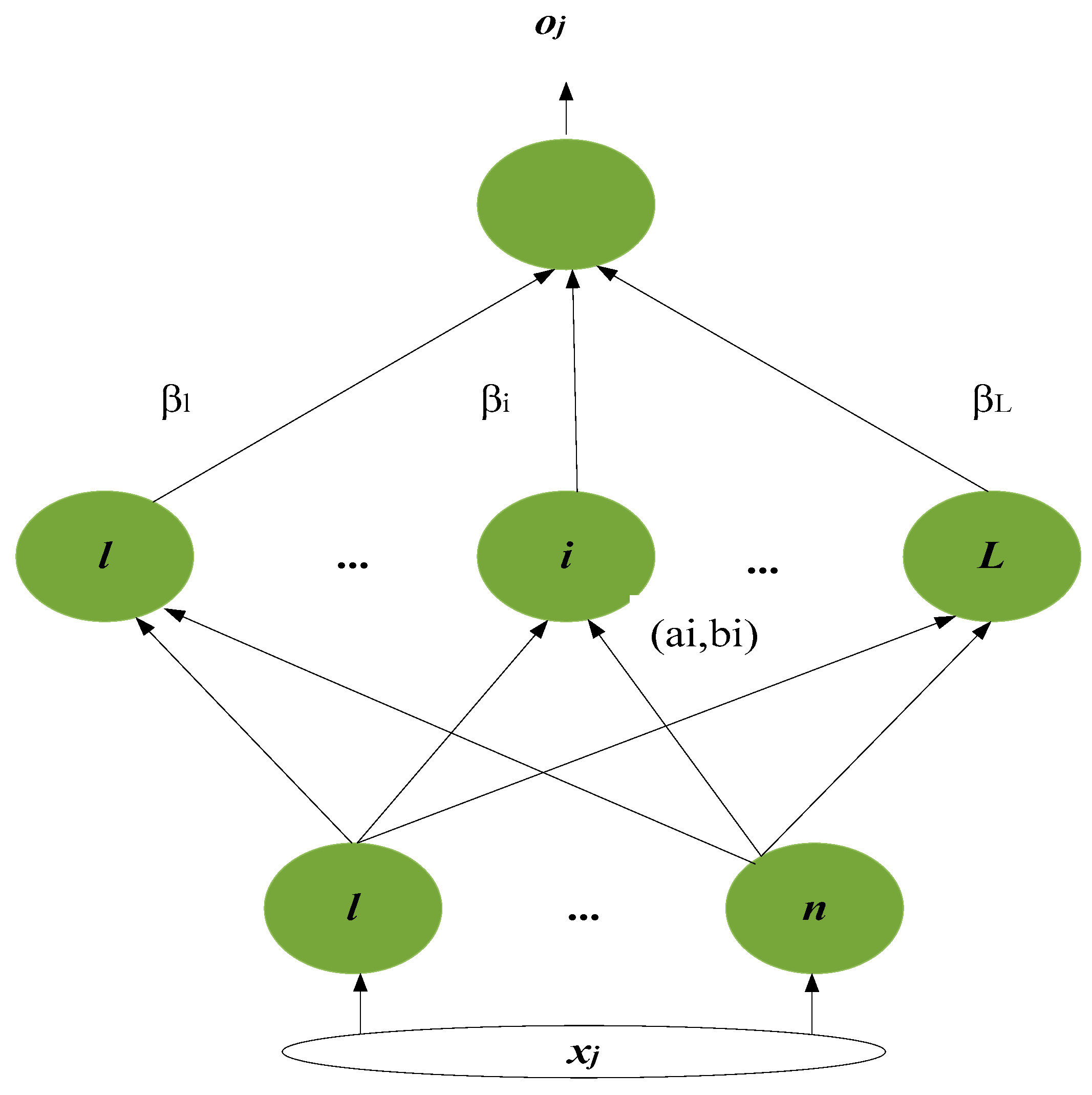
2.3. The Multi-Kernel Extreme Learning Machine

The MKELM method transfers the low dimensional data into Hilbert space to reduce the randomness and complexity of the model network through regularization theory and kernel mapping based on the extreme learning machine (ELM) and kernel extreme learning machine (KELM), which can effectively improve the prediction accuracy and generalization ability of the model.

The ELM is a new machine learning method proposed by Professor Huang of Nanyang Polytechnic University in Singapore [72]. Its structure is shown in Figure 3. The ELM is an effective single hidden layer feedforward network, which only needs to set the number of hidden layer nodes in the network structure without adjusting the network input weights and bias values. Compared with neural network and other methods, the ELM method has superior prediction performance and better generalization ability in classification and regression prediction.

Given N training samples, where $\left(x_i,t_i\right)$ is the input value of the electricity-heat-cooling-gas loads samples, $x_i=[x_{i1},x_{i2},\cdots ,x_{in}]$ is the expected output value of the electricity-heat-cooling-gas loads samples, and the amount of hidden nodes of the ELM model is L, then the output should be

$$f_L(x_j)={\displaystyle \sum _i^L\beta G\left(a_i,b_i,x_j\right)=h\left(x_j\right)}\beta$$

(8)

where $\beta$ is the output weight from hidden node to output node, G represents the motivation function, $a_i$ and $b_i$ are the parameters of i-th hidden layer, and $h\left(x_j\right)$ is the output vector of the hidden layer.

Furthermore, it can be expressed by matrix expression of linear system as

$$H\beta =T$$

(9)

Among Equation (9),

$$\{\begin{array}{l}H\left(a_1,\cdots ,a_L;b_1,\cdots ,b_L;x_1,\cdots ,x_N\right)\\ \begin{array}{cc}& \end{array}={\left[\begin{array}{ccc}G\left(a_1,b_1,x_1\right)& \cdots & G\left(a_L,b_L,x_1\right)\\ ⋮& ⋮& ⋮\\ G\left(a_1,b_1,x_N\right)& \cdots & G\left(a_L,b_L,x_N\right)\end{array}\right]}_{N\times L}\\ \beta ={\left[\begin{array}{l}{\beta }_1^T\\ {\beta }_2^T\\ ⋮\\ {\beta }_L^T\end{array}\right]}_{L\times d};T={\left[\begin{array}{l}{t}_1^T\\ t_2^T\\ ⋮\\ t_L^T\end{array}\right]}_{N\times d}\\ \end{array}$$

(10)

In the ELM model, if the motivation function is infinitely differentiable, the bias value and input weight of the structure do not need to be changed, and then the ELM training problem can be transformed into solving $\beta$. The least square method is usually used to determine the output weight of the ELM model:

$$\widehat{\beta }=H^{+}T=H^T{\left(H{H}^T\right)}^{-1}T$$

(11)

where $H^{+}$ is the Moore Penrose generalized inverse of the hidden layer output matrix $H$ [73].

When solving $H^{+}$, the sample data set may have multi-collinearity problem, which may lead to non-singularity, and then have a certain impact on the prediction results. Considering this, the parameter 1/C is introduced into diagonal matrix $H{H}^T$ to make the characteristic root of $H{H}^T$ deviate from zero. Therefore, the weights $\beta$ of the ELM model can be solved through Equation (12) [74].

$$\beta =H^T{\left(\frac{1}{C}+H{H}^T\right)}^{-1}T$$

(12)

The ELM model can effectively avoid the problems of slow calculation speed and overfitting of a traditional neural network, since it does not need to train a large number of model parameters in the training process. However, there also exist disadvantages in the ELM model. For example, the process of selecting the number of hidden nodes is complicated and time-consuming, which needs a lot of experiments or subjective experience to select the optimal number of neurons resulting in the decline of prediction performance and generalization ability of the model.

Aiming at solving this demerit, Professor Huang proposed the KELM model, which can effectively avoid the selection of hidden layer. By transforming the output vector of hidden layer into kernel function mapping of support vector machine, the output random fluctuation is reduced, and the generalization ability and robustness of the model are improved [72].

The definition of the kernel matrix in the KELM model is

$${\mathsf{\Omega }}_{ELM}=H{H}^T:{\mathsf{\Omega }}_{ELMij}=h(x_i)•h(x_j)=K(x_i,x_j)$$

(13)

where ${\mathsf{\Omega }}_{ELM}$ is the kernel matrix of the KELM model and $K(x_i,x_j)$ is the kernel function.

Then, Equation (12) can be transformed into

$$\beta =H^T{\left(\frac{1}{C}+{\mathsf{\Omega }}_{ELM}\right)}^{-1}T$$

(14)

Therefore, the output expression of the KELM model can be written as [74]

$$f(x)=h(x)H^T{\left(\frac{1}{C}+H{H}^T\right)}^{-1}T=\left[\begin{array}{l}K(x_{},x_1)\\ ⋮\\ K(x_{},x_N)\end{array}\right]{\left(\frac{1}{C}+{\mathsf{\Omega }}_{ELM}\right)}^{-1}T$$

(15)

Generally, the KELM model provides various selections of kernel functions, such as Poly kernel, Gaussian RBF kernel, etc. The selection of the kernel function has a great impact on the forecasting results of the combined electricity-heat-cooling-gas loads. The single kernel model is usually difficult to adapt to the samples with multiple data characteristics. Hence, to overcome the shortcomings and limitations of single KELM, this paper combines different kernel functions and makes full use of the advantages of different kernel functions in learning and generalization, and constructs a multi-kernel extreme learning machine model.

According to Equation (15), the selection of kernel function has a significant influence on the prediction results of the model. Kernel functions are divided into global kernel (such as RBF kernel function) and local kernel (such as poly kernel function), which are

$$K_{RBF}(x,x_i)=\exp \left(\frac{-{\Vert x-x_i\Vert }^2}{{\delta }^2}\right)$$

(16)

$$K_{Poly}(x,x_i)={\left(x•x_i+1\right)}^d$$

(17)

where $\delta$ is the kernel parameter of the RBF kernel function and $d$ is the kernel parameter of the Poly kernel function [75,76].

The data characteristic distribution of RBF kernel function and Poly kernel function when x = 0 and x = 0.5 are provided in Figure 4 and Figure 5. From Figure 4, it can be found that the RBF kernel function can make the near data affect the kernel value, and has better local learning ability, but it has the disadvantage of poor generalization performance. The Poly kernel function can identify the influence of remote data on kernel value, and its global generalization ability is strong. However, when the data is concentrated to the central point, the influence of remote data on kernel value is significantly reduced, and its learning ability becomes weak. Therefore, it can be seen that the identification ability of different kernel functions for sample data features is quite different. As the integrated embodiment of multiple influencing factors, the electricity-heat-cooling-gas load is a dynamic evolution process of multiple data features including trend characteristics, periodic characteristics, volatility characteristics, and chaotic characteristics. Thus, it is difficult to use a single kernel function to make a high-precision regression prediction for the electricity-heat-cooling-gas load with multiple data distribution characteristics. Considering this, this paper combines the RBF kernel function and the Poly kernel function to construct a hybrid kernel function, so as to integrate the superior learning ability and generalization ability of the two kernel functions. Based on the Mercer theory, the kernel matrix satisfies semi-positive definiteness, which means the linear combination of multiple single kernel functions is still a kernel function. Based on this, the hybrid kernel function is constructed as follows

$$K(x,x_i)=\rho K_{RBF}(x,x_i)+\left(1-\rho \right)K_{Poly}(x,x_i)$$

(18)

where $\rho$ is the weight coefficient of $K_{RBF}(x,x_i)$ in the hybrid kernel function and $\left(1-\rho \right)$ is the weight coefficient of $K_{Poly}(x,x_i)$ in the hybrid kernel function, which can adjust the mapping ability of the hybrid kernel function.

The MKELM model can be constructed by introducing the Equation (18) into the Equation (15). The parameters need to be determined including regularization coefficient C, RBF kernel parameter $\delta$, Poly kernel parameter $d$, and weight coefficient $\rho$. In this paper, the improved SSA bionic intelligent optimization algorithm is used to optimize these four parameters.

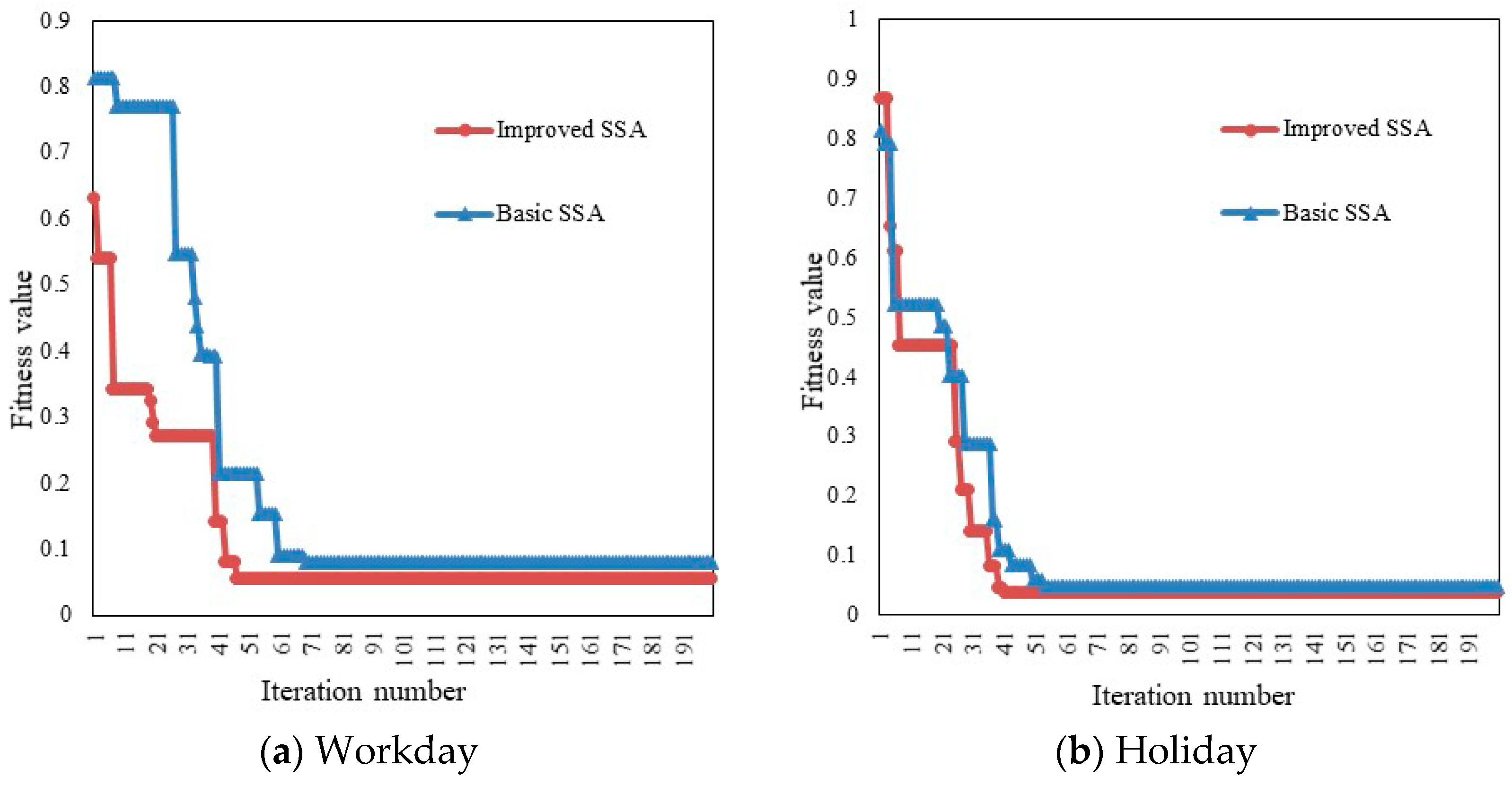
2.4. The Improved SSA

The Salp Swarm Algorithm (SSA) is a new heuristic optimization algorithm proposed by an Australian scholar named Seyedali Mirjalili in 2017 [77]. It is proposed by imitating the behavior of the chain group of the salp in the process of looking for food. A single salp and a salp chain are shown in Figure 6.

In the SSA, the initial population is divided into leader and follower. The leader leads the Salp chain. The specific steps of the SSA are as follows.

(1)

Parameters setting

Five parameters need to be set in the SSA, which are the initial population number Agents_no, the amount of variables dim, the maximum number of iteration Max_iteration, the lower bound of variables $lb=\left[l{b}_1,l{b}_2,\cdots \right]$, and the upper bound of variables $ub=\left[u{b}_1,u{b}_2,\cdots \right]$.

(2)

Population initialization

The position of the initial population in the SSA is set randomly, and the position matrix of the salp swarm S is as follows

$$S=\left[\begin{array}{cccc}{s}_{11}& s_{12}& \cdots & s_{1d}\\ s_{21}& s_{22}& \cdots & s_{2d}\\ ⋮& ⋮& ⋮& ⋮\\ s_{n1}& s_{n2}& \cdots & s_{nd}\end{array}\right]$$

(19)

where $s_{ij}$ represents the value of the j-th variable of the i-th salp, $i=1,2,\cdots ,n$, $j=1,2,\cdots ,d$.

$s_{ij}$ can be calculated by Equation (20) with random distribution:

$$S(i,j)=rand(i,j)\times (ub(i)-lb(i))+lb(i)$$

(20)

where $S\left(i,j\right)$ demonstrates the value of the i-th row and j-th column in the matrix $s_{ij}$, rand(i, j) implies the random matrix, and ub(i) and lb(i) mean the upper bound and the lower bound of the i-th salp, respectively.

(3)

Fitness function construction

The fitness function is written as follows:

$$OS=\left[\begin{array}{c}OS1\\ OS2\\ ⋮\\ OSn\end{array}\right]=\left\{\begin{array}{c}f\left[\left(\begin{array}{cccc}{s}_{11}& s_{12}& \cdots & s_{1d}\end{array}\right)\right]\\ f\left[\left(\begin{array}{cccc}{s}_{21}& s_{22}& \cdots & s_{2d}\end{array}\right)\right]\\ ⋮\\ f\left[\left(\begin{array}{cccc}{s}_{n1}& s_{n2}& \cdots & s_{nd}\end{array}\right)\right]\end{array}\right\}$$

(21)

In the matrix OS, the position of the salp with the best fitness value is designated as the variable F as the source food, which is tracked by the salp chain.

(4)

Iteration

In the SSA, all the salp will change their positions to perform global search and avoid local optimization. Leaders update the location of food sources as shown below:

$$x_j^1=\{\begin{array}{l}{F}_j+c_1\left(u{b}_j-l{b}_j\right)c_2+l{b}_j\begin{array}{cc}& c_3\ge 0\end{array}\\ F_j-c_1\left(u{b}_j-l{b}_j\right)c_2+l{b}_j\begin{array}{cc}& c_3<0\end{array}\end{array}$$

(22)

where $x_j^1$ represents the position of the first salp (leader) in the j-th dimension, $F_j$ is the position of the food source, $u{b}_j$ and $l{b}_j$ demonstrate the upper bound and lower bound, respectively, and $c_1$, $c_2$, and $c_3$ are random constants. $c_2$ and $c_3$ are generated randomly in the interval [0, 1], which determine the iteration direction of the next position of the j-th dimension and step length. $c_1$ is a critical parameter in the SSA, and the definition is as below:

$$c_1=2e^{-{\left(\frac{4l}{L}\right)}^2}$$

(23)

where l is the current number of iterations and L is the maximum number of iterations.

The SSA uses Newton’s law of motion to update the follower’s position as

$$x_j^i=\frac{1}{2}a{t}^2+v_{0}t=\frac{1}{2}\frac{v_{final}}{v_0}{t}^2+v_{0}t$$

(24)

where $x_j^i$ is the position of the i-th follower in the j-th dimension, t means the time, $v_0$ represents the initial velocity and $i\ge 2$.

In the SSA, all steps are executed in the iteration process until reaching the end standard of the SSA iteration, except initialization.

In order to further improve the optimization performance of the SSA and make it better for solving the optimization problem of high-dimensional complex parameters in the MKELM prediction model, this paper introduces dynamic inertia weight and chaotic local searching mechanism into the basic SSA intelligent optimization algorithm, which named improved SSA (ISSA) in this paper, so as to improve the optimization searching speed of the SSA and avoid falling into local optimum easily.

It can be seen from Equation (22) that the leader updates the position according to the information position of the parent generation in the iteration process, which mainly focuses on the area near the existing individuals.

As a result, the search scope of the algorithm is limited, leading to the oscillation phenomenon in the later optimization stage, which will reduce the convergence accuracy and convergence speed of the SSA. In order to solve this problem, inertia weight mechanism is introduced into the SSA, which can control the balance between global searching and local searching of the whole algorithm by adjusting its own value, so as to strengthen the convergence ability of the algorithm. Therefore, the inertia weight mechanism is introduced on the basis of the Equation (22), and the updated equation is obtained as below:

$$x_j^1=\{\begin{array}{l}w{F}_j+c_1\left(u{b}_j-l{b}_j\right)c_2+l{b}_j\begin{array}{cc}& c_3\ge 0\end{array}\\ w{F}_j-c_1\left(u{b}_j-l{b}_j\right)c_2+l{b}_j\begin{array}{cc}& c_3<0\end{array}\end{array}$$

(25)

where w is the inertia weight, which can control the influence of parent position information on the new population, so as to adjust the searching trend and expand the searching scope. Generally speaking, using a larger weight in the early stage of the iteration will help to quickly locate the range of the optimal solution, and the convergence speed of the algorithm can be accelerated by reducing the weight in the later stage of the iteration. It is difficult to make optimal adjustment according to the population optimization and iteration by using fixed inertia weight. Therefore, the dynamic inertia weight with nonlinear time-varying updating is employed in this paper to improve the basic SSA.

$$w={\left(\frac{2}{t}\right)}^{0.3}$$

(26)

where t is the number of iteration steps of the current population.

With the increase of iteration steps, the inertia weight between individuals decreases from the initial value, which can avoid the oscillation phenomenon of the SSA in the later stage of optimization and accelerate the population convergence speed of the SSA.

Generally speaking, when the SSA enters the later stage of the optimization iteration, the population tends to approach the local optimum. Chaotic motion has the advantages of regularity and ergodicity, which can traverse all states in the specified range without repetition. Therefore, in order to further enhance the optimization performance of the SSA, the chaotic local searching strategy is introduced into the SSA to reduce the shortcoming of easily falling into local optimum and improve the searching efficiency of the SSA in the solution space. The specific process of introducing chaotic local searching strategy into the SSA is as follows.

(1)

The individual $s_{ij}$ is generated into chaotic variables as

$${\phi }_i^j=\left(s_{ij}-s_i^{\min }\right)/\left(s_i^{\max }-s_i^{\min }\right)$$

(27)

where ${\phi }_i^j$ is the chaotic variable, $s_i^{\min }$ and $s_i^{\max }$ are the minimum value and maximum value of the j-th variable.

(2)

Generating chaotic sequence by logic mapping as

$${\phi }_{i+1}^j=4{\phi }_i^j\left(1-{\phi }_i^j\right)$$

(28)

(3)

The chaotic sequence is transformed into the searching space of the target solution to generate a new position, and compared with the group optimal individual. The better value is selected to update, so as to complete the local searching process. This procedure can be written as

$$s_{i+1}^j=s_i^{\min }+{\phi }_{i+1}^j\left(s_i^{\max }-s_i^{\min }\right)$$

(29)

The improved SSA has been enhanced in global searching and local searching, hence it has higher convergence accuracy and better optimization performance. The improved SSA can also help the MKELM prediction model to explore the optimal parameters values to improve the accuracy in the combined electricity-heat-cooling-gas loads prediction.

2.5. The Established Uncertain Interval Forecasting Model for the Combined Electricity-Heat-Cooling-Gas Loads in the IES

The established uncertain interval forecasting model of the combined electricity-heat-cooling-gas loads on the demand side in the IES contains the Bootstrap method, the MTL method, and the MKELM optimized by the improved SSA. The role of each method is illustrated in Figure 7. The specific modeling steps of the uncertain interval forecasting model are described as below.

(1)

The selection of model variables and the preprocessing of sample data

According to the characteristics of the combined electricity-heat-cooling-gas loads forecasting, the input variables of the forecasting model are selected, which are the primary factors influencing the demand of the electricity-heat-cooling-gas loads, including weather, calendar information, social-economic factors, and historical load. Considering that each variable has different units, the sample data of the selected variables are normalized as the Equation (30), so that they can be analyzed in the same dimension.

$${\widehat{x}}_i=\frac{x_i-\underset{i}{\min }(x)}{\underset{i}{\max }(x)-\underset{i}{\min }(x)}$$

(30)

where ${\widehat{x}}_i$ is the standardized value, $x_i$ is the sample value, and min(x) and max(x) are the minimum value and maximum value, respectively.

(2)

Sample division

The sample data is classified into training sample data and testing sample data to construct the training set and testing set for the combined electricity-heat-cooling-gas loads forecasting model. Additionally, then the Bootstrap method is employed to construct M pseudo sample sets by repeated sampling.

(3)

Multi-tasks construction

There exist strong coupling relations among electric energy subsystem, heat energy subsystem, cooling energy subsystem, and gas energy subsystem in the IES as description in Section 2. The load demand of each energy subsystem is related and influenced each other, which is suitable to employ the MTL method. Therefore, the MTL method is incorporated into the uncertain interval forecasting model for the electricity-heat-cooling-gas loads. Hence, four single tasks can be constructed according to the load demand characteristics of electricity, heat, cooling, and gas, which can be fed into the model as a module in the prediction model.

(4)

Parameters setting of the ISSA and the optimal values for the parameters in the MKELM

The parameters of the ISSA algorithm are set, and the regularization coefficient C, the RBF kernel parameter $\delta$, the poly kernel parameter $d$ and the weight coefficient $\rho$ in the MKELM model are optimized by using the ISSA, and the optimal values of these four parameters are finally determined. The root mean square error (RMSE) of the prediction results is utilized as the fitness function of the improved SSA, which can be calculated as Equation (31).

$$RMSE=\sqrt{\frac{1}{n}{\displaystyle \sum _{k=1}^n{(y(k)-\widehat{y}(k))}^2}}$$

(31)

Additionally, the group position of the ISSA is updated according to Equation (25). The chaotic local searching is carried out for the population optimal solution in a single iteration employing Equations (27)–(29). When the termination condition is reached, the optimization of the ISSA is completed, and then the optimal values of four parameters in the MKELM model can be obtained.

(5)

Uncertain interval prediction

The optimal values of four parameters in the MKELM model are input into the MKELM model. The MKELM model is trained according to M pseudo sample sets and the expected values of the prediction results of the pseudo sample sets are taken as the point prediction results of the MKELM model. The error variance of the MKELM model is calculated according to the Equation (3). The noise variance set is constructed employing the Equation (5) and the fitness function is obtained according to the Equation (6) which calculates the noise variance through training the MKELM model by the ISSA. Thus, the forecasting interval of the combined electricity-heat-cooling-gas loads can be constructed according to Equation (7).

(6)

Forecasting performance evaluation

The performance of the proposed uncertain interval forecasting model for the combined electricity-heat-cooling-gas loads is evaluated by two indicators, which are the prediction interval coverage probability (PICP) and the prediction interval normalized averaged width (PINAW). The PICP represents the probability that the forecast interval covers the actual electricity-heat-cooling-gas loads. The larger the PICP, the higher the reliability of the interval obtained by the prediction model is, which can better avoid the electricity-heat-cooling-gas loads from exceeding the upper and lower limits of the prediction interval. The PINAW demonstrates the uncertainty degree of the prediction interval of the model. The narrower the width, the lower the uncertainty of the prediction interval and the better the accuracy of the model. The calculation process of the PICP and PINAW are shown in Equations (32) and (33).

$$PICP=\frac{1}{N}{\displaystyle \sum _{i=1}^N{b}_i}$$

(32)

$$PINAW=\frac{1}{NR}{\displaystyle \sum _{i=1}^N\left(U\left(x_i\right)-L\left(x_i\right)\right)}$$

(33)

where N is the number of testing samples for the electricity-heat-cooling-gas loads prediction, R is the range of the target values defined as the difference between its minimum and maximum values, $U\left(x_i\right)$ and $L\left(x_i\right)$ are the upper and lower bounds of the i-th prediction interval of the electricity-heat-cooling-gas loads, and $b_i=1$, if the actual load value is contained in the prediction interval, otherwise, $b_i=0$.

The calculation process of the established uncertain interval forecasting model for the combined electricity-heat-cooling-gas loads in the IES is illustrated in Figure 8.

3. Results

Aiming at verifying the feasibility and effectiveness of the established uncertain interval forecasting model for the combined electricity-heat-cooling-gas loads in the IES, the industrial park in northern China is selected as the research object for empirical analysis. The internal energy supply and demand structure of this industrial park is illustrated in Figure 1. The IES of the selected industrial park is composed of electric energy subsystem, heat energy subsystem, cooling energy subsystem, and gas energy subsystem, including CCHP unit, Photovoltaic unit, electric boiler, gas boiler, electric refrigerator, absorption refrigerator, other energy generation and conversion equipment, as well as electric energy storage, heat storage and other energy storage equipment to improve the operation flexibility and operation economy of the IES.

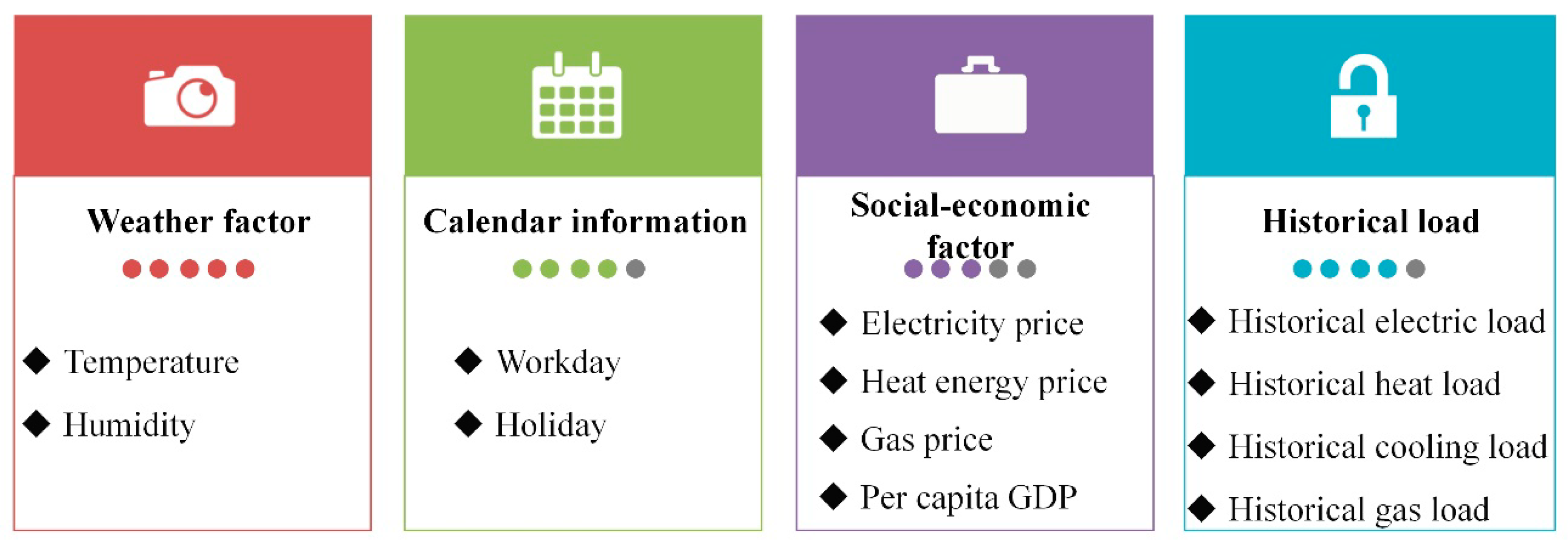
3.1. Variables Selection and Data Preprocess

In the application of the established uncertain interval forecasting model for the electricity-heat-cooling-gas loads in the IES, four factors, namely, weather, calendar information, social-economic factors, and historical load, are considered as the input variables of the forecasting model. The specific variables of four factors are listed in Figure 9. As can be seen from Figure 9, the weather factor contains the temperature index and humidity index. The calendar information factor includes workday and holiday (weekends included). The social–economic factor is the critical factor of the combined load prediction of the IES which is consisted of electricity price, heat energy price, gas price, and per capita GDP. The historical load is made up of historical load data of each energy subsystem, including historical electric load, historical heat load, historical cooling load, and historical gas load.

The hourly data of different variables from January 2018 to June 2018 are selected as the training sample, and the hourly data of different variables of July 2018 is treated as the test sample for the established uncertain interval forecasting model of the industrial park’s combined electricity-heat-cooling-gas loads. The data are collected from the Meteorological Bureau and Energy statistics of the province where the industrial park located and through site investigation. Additionally, Matlab R2014a is employed for programming.

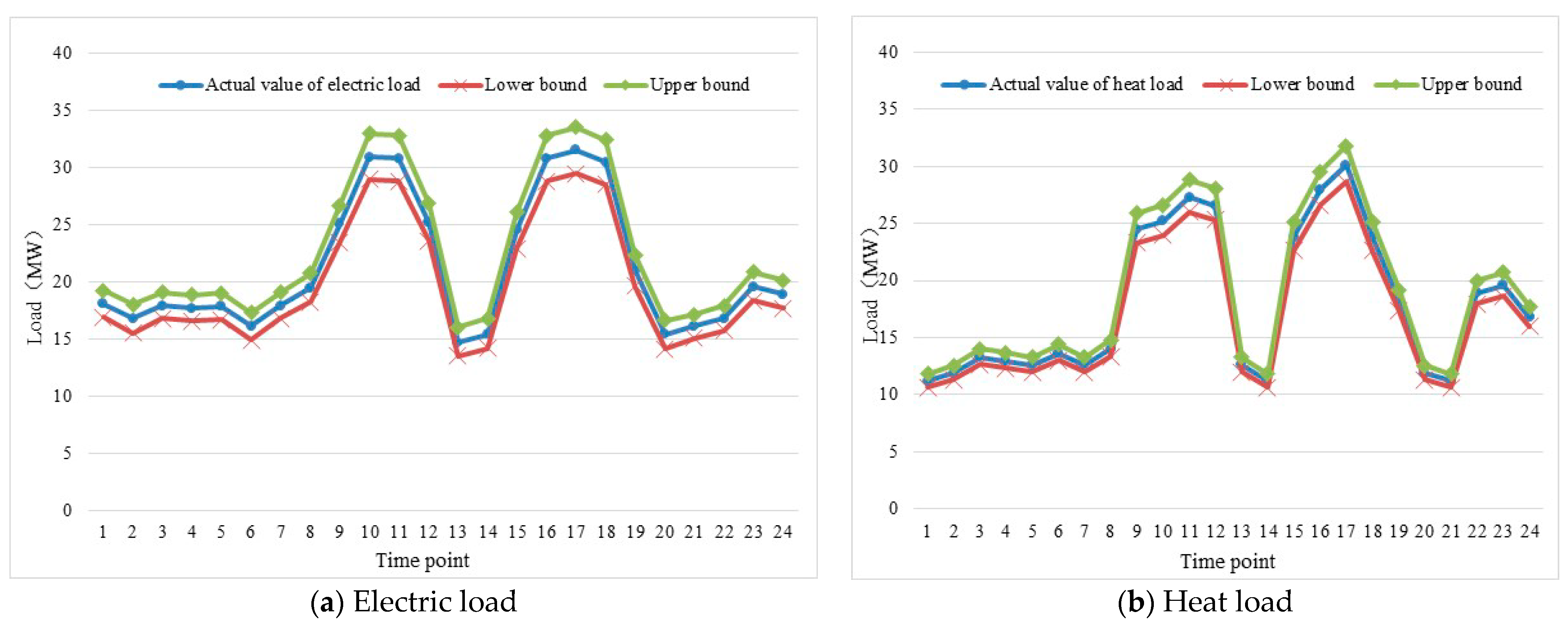
3.2. Forecasting Results Analysis

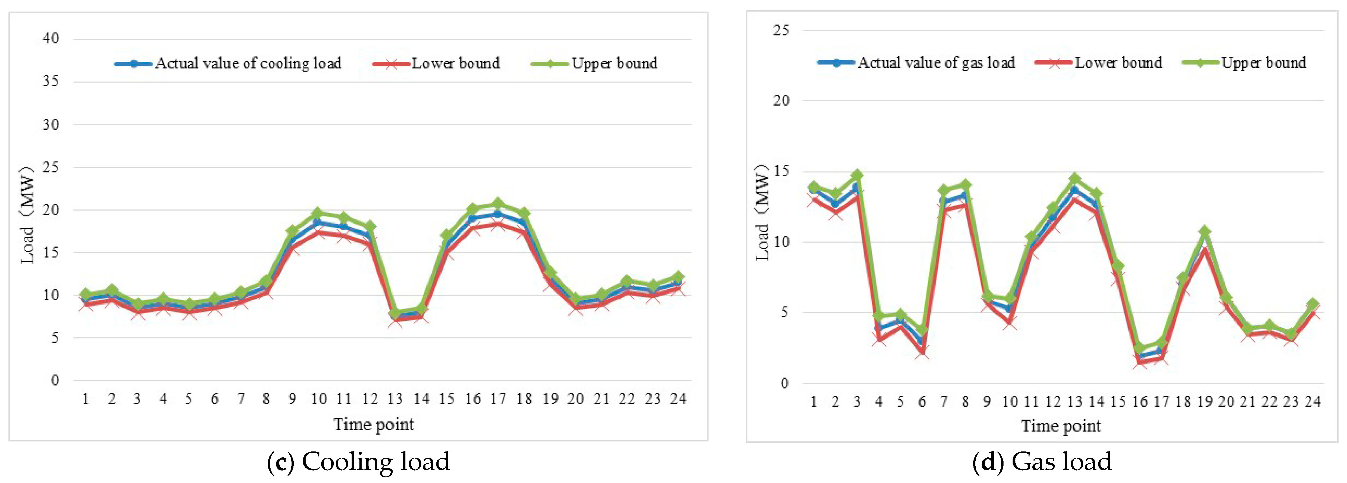
Before forecasting the electricity-heat-cooling-gas loads in the IES of the industrial park, it is necessary to determine the parameters of the ISSA. Specifically, Agents_no = 100, dim = 4, Max_iteration = 200, and the lower and upper bounds of variables are 0 and 10. This paper selects a workday (2018.07.12) and a holiday (2018.07.22) as the testing objects. The ISSA is employed to optimize the parameters of the MKELM, including regularization coefficient C, RBF kernel parameter $\delta$, Poly kernel parameter $d$, and weight coefficient $\rho$, and the optimization results are shown in

Table 1. Parameter optimization results of the MKELM model.

Parameters	C	$\rho$	$\delta$	$d$
Workday (2018.07.12)	1.58	0.34	0.77	2.89
Holiday (2018.07.22)	1.94	0.51	0.43	2.14

.

Figure 10 shows the iterative optimization convergence curve of the ISSA and the basic SSA in finding the optimal parameters values of the MKELM model. It can be seen that the ISSA converges in steps 50 and 41 on workday and holiday, respectively, while the basic SSA converges in steps 69 and 54, respectively. Moreover, the fitness function values of the ISSA in workday and holiday are 0.054 and 0.038, respectively, which are better than those of the basic SSA (0.079 and 0.047, respectively). Therefore, compared with the basic SSA, the ISSA has higher convergence accuracy and convergence speed. The main reason is that the ISSA can effectively solve the oscillation problem of the basic SSA in the iterative convergence process by introducing the dynamic inertia weight mechanism, thus improving the stability and searching efficiency of the algorithm. At the same time, the chaotic local searching mechanism is introduced into the basic SSA, which can reduce the risk of the SSA falling into local optimum, and improve the optimization performance of the SSA.

Furthermore, according to the established uncertain interval forecasting model of the combined electricity-heat-cooling-gas loads in the IES, the forecasting intervals of various loads on workday and holiday at 90% confidence level can be obtained, as shown in Figure 11 and Figure 12.

According to the above prediction results, it can be deduced that:

(1)

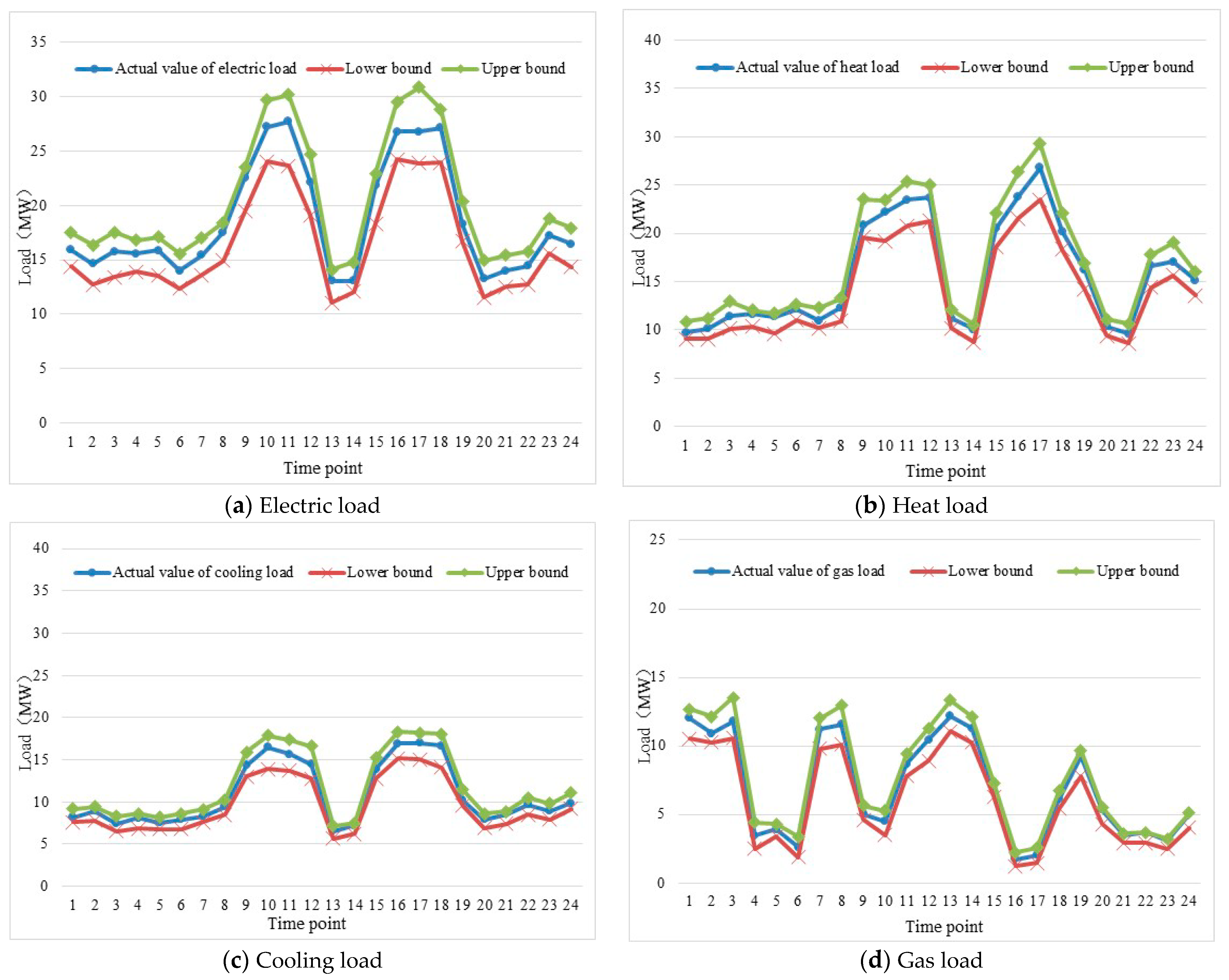
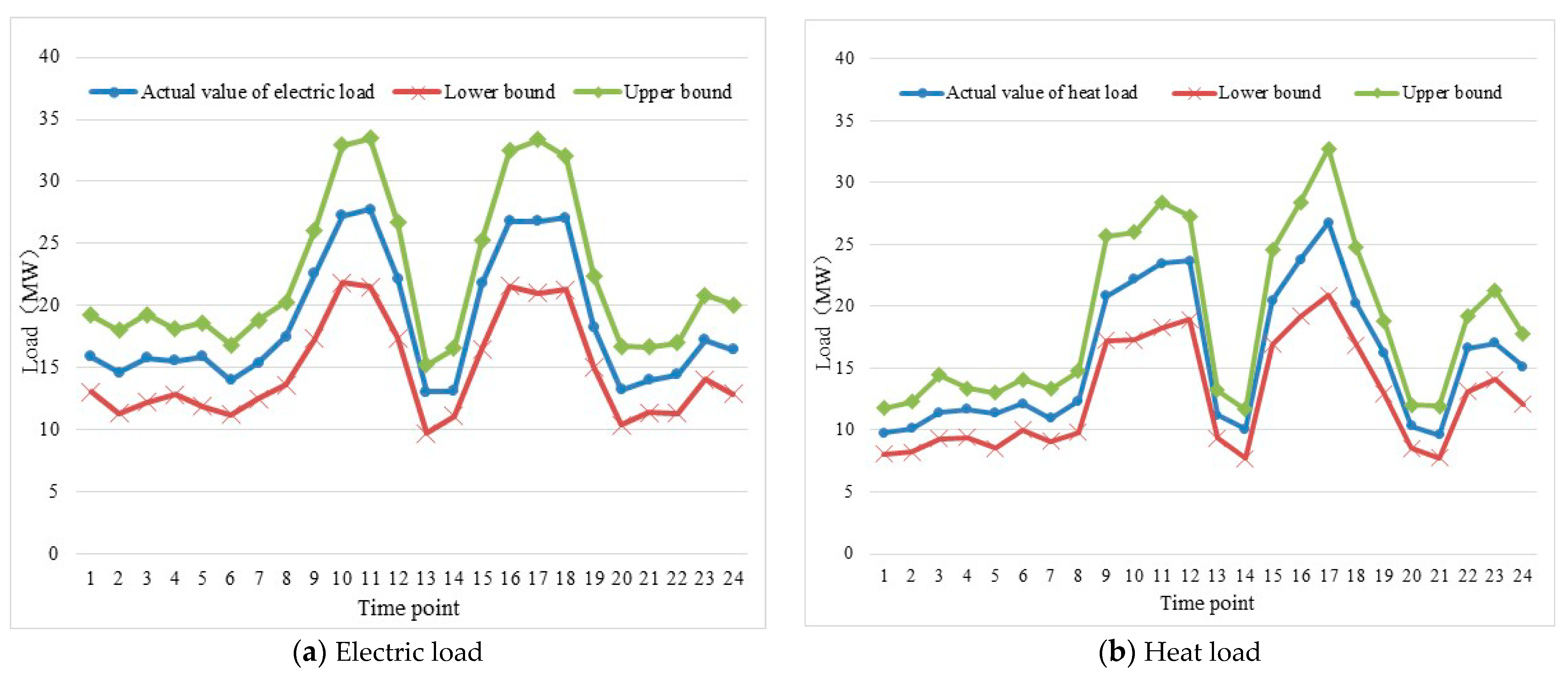
Electric, heat, cooling, and gas loads have peak, flat, and valley periods, but the number of peak, flat, and valley is different. The prediction results of the uncertain interval forecasting model established in this paper can better reflect the fluctuation characteristics of various loads. However, generally, the prediction interval is relatively large in the peak and valley periods, which indicates that the load is often difficult to predict at the time point with large fluctuation.

(2)

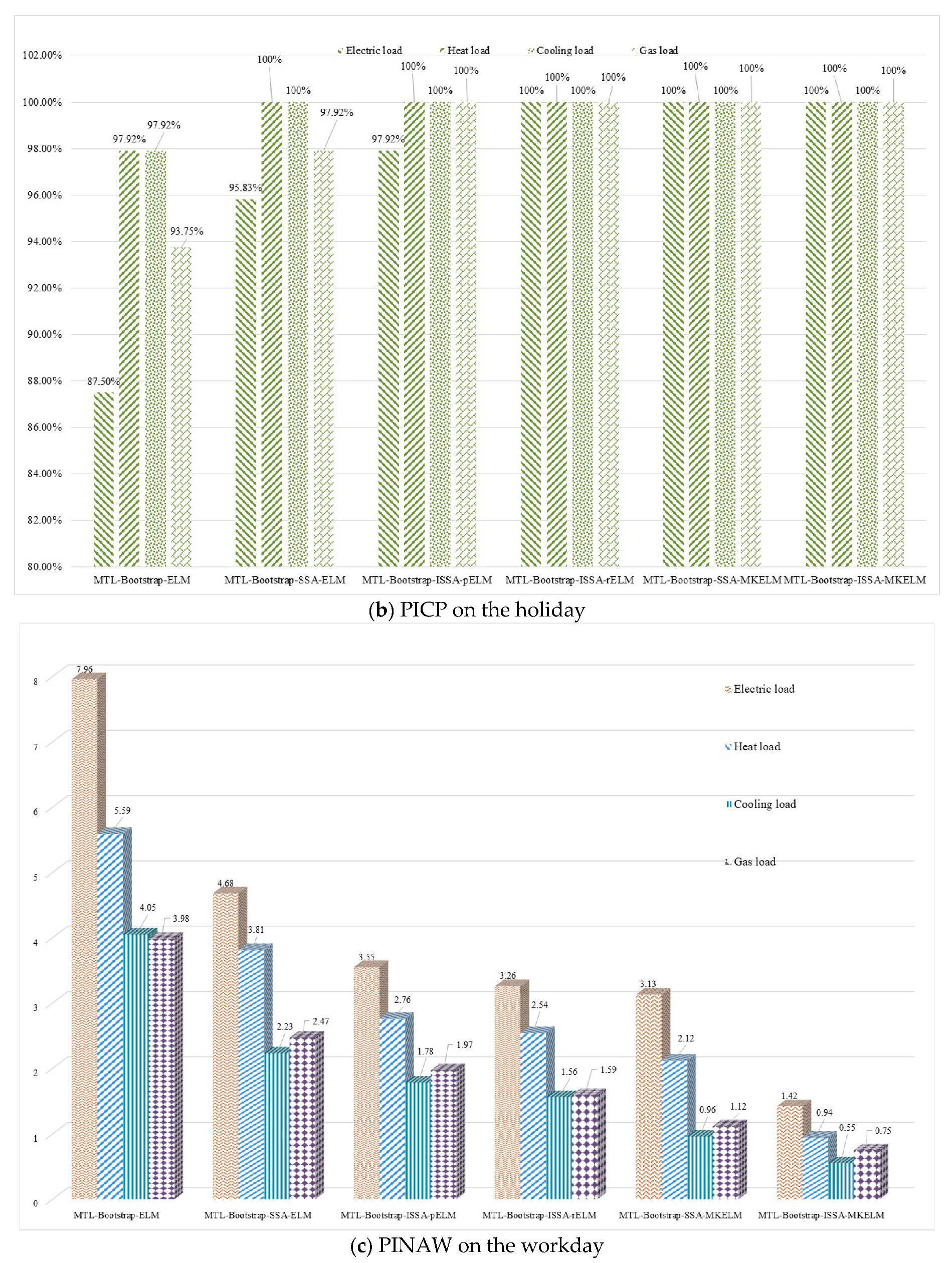
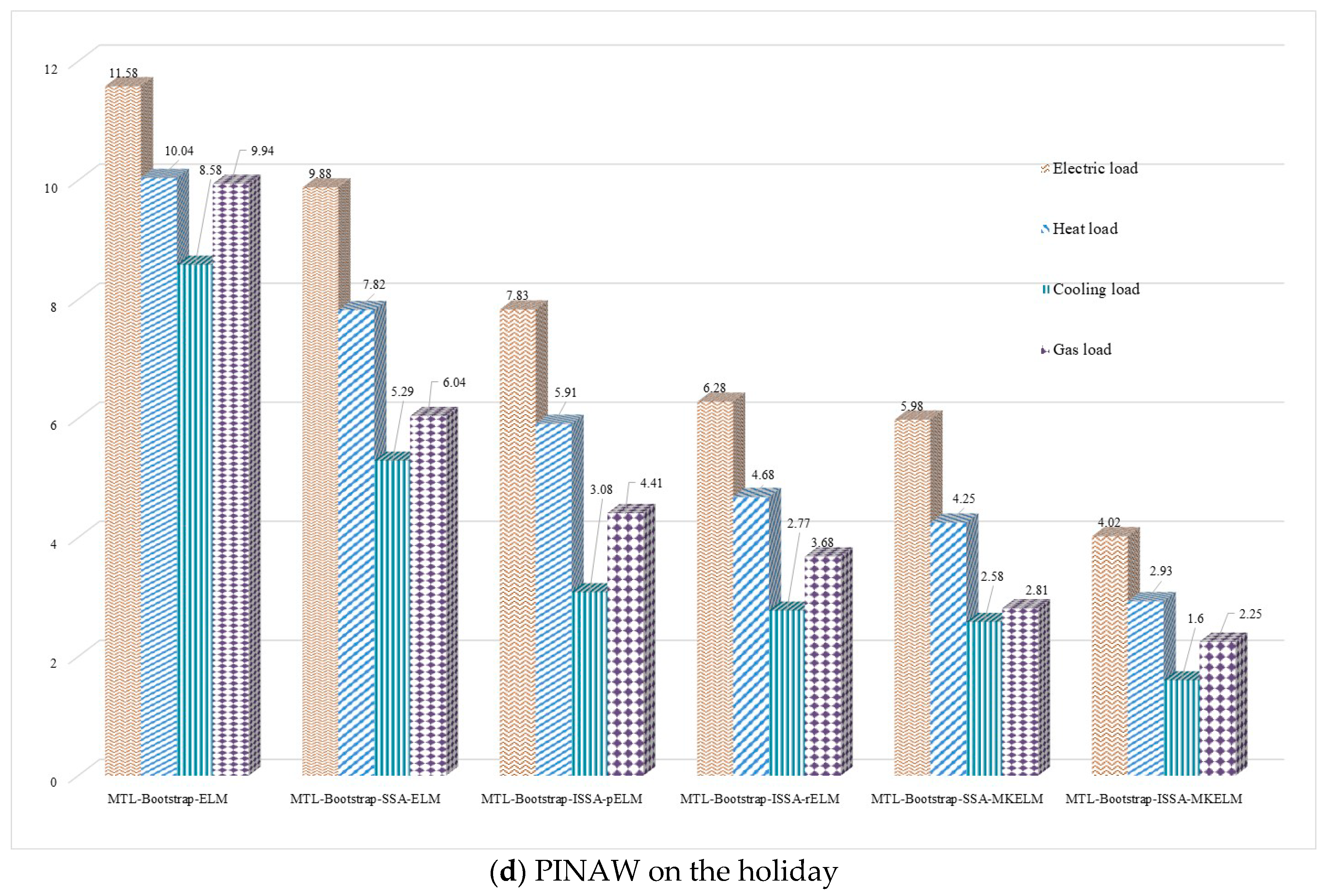
The electric load, heat load, and gas load fluctuate greatly, but the prediction interval of electric load is large. The PINAW values of electric load prediction on a workday (July 12) and holiday (July 22) are 1.42 MW and 4.02 MW, respectively, while the PINAW values of heat load, gas load, and cooling load prediction on workday (July 12) and holiday (July 22) are 0.94 MW and 2.93 MW, 0.55 MW and 1.60 MW, as well as 0.75 MW and 2.25 MW, respectively. This is mainly because the inertia of heat load, gas load, and cooling load is stronger than that of electric load, and the characteristics of easy storage for heat load, cooling load, and gas load can provide more flexible backup for the IES of industrial park, which makes the prediction interval of heat load, cooling load, and gas load relatively small.

(3)

Although the fluctuation of electric, heat, cooling, and gas load is various on a workday (July 12) and holiday (July 22), the forecasting results of the workday are better than those of the holiday. The PICP values of electric, heat, cooling, and gas loads prediction are all 100% on the workday and holiday, while the PINAW values of electric, heat, cooling, and gas loads prediction on the workday are 1.42 MW, 0.94 MW, 0.75 MW, and 0.55 MW, respectively, which are 64.76%, 67.85%, 66.64%, and 65.75% lower than those on the holiday (the PINAW values of electric, heat, cooling, and gas load prediction on holiday are 4.02 MW, 2.93 MW, 2.25 MW, and 1.60 MW, respectively). The multi-energy loads demand on holiday has more uncertainties, therefore, it is much more difficult to carry out accurate load forecasting.

4. Discussion

In order to verify the effectiveness and forecasting accuracy of the established uncertain interval prediction model, including the MTL method, the Bootstrap method, the MKELM method, and the ISSA, for the combined electricity-heat-cooling-gas loads in the IES, the STL method as well as some other optimization algorithms and other kernel functions of the ELM are selected to comparatively discuss about the prediction accuracy.

4.1. Comparison Discussion on the Forecasting Results Obtained by the MTL Method and STL Method

There exist strong coupling relations among electric, heat, cooling, and gas loads in the IES, therefore, the MTL method is suitable for the uncertain interval prediction multi-energy loads. According to the prediction results in the previous section, it can be seen that the multi-load uncertain interval prediction model containing the MTL method has superior prediction performance. In order to further verify the effectiveness and feasibility of the MTL method, the STL method is employed to replace the MTL method in the established uncertain interval prediction model, hence we can comparatively analyze the prediction results obtained by the STL method and the MTL method. In order to ensure the comparability of the prediction results, the same input sample data, output sample data, and the model parameter values are used for the two kinds of prediction models with different task types. The difference is that in the multi-load uncertain interval prediction model of the IES with the STL method, electric load, heat load, cooling load, and gas load will be input into the model for prediction, respectively, while in the model with the MTL method, electric load, heat load, cooling load, and gas load will be input into the model at the same time, and the uncertain interval prediction results of the four kinds of loads can be obtained by one time.

The prediction results of the multi-load uncertain interval prediction model of the IES with the STL method on workday (July 12) and holiday (July 22) are shown in Figure 13 and Figure 14.

The prediction performance of the multi-load uncertain interval prediction model for the IES of the industrial park with the STL method and the MTL method is shown in

Table 2. Prediction performance comparison of two models with the STL method and the MTL method.

Method	Workday (July 12) Electric Load		Holiday (July 22) Electric Load		Workday (July 9–13) Electric Load		Holiday (July 21–22) Electric Load
	PICP	PINAW	PICP	PINAW	PICP	PINAW	PICP	PINAW
Model with the STL	100%	2.99	100%	7.66	100%	3.02	100%	7.68
Model with the MTL	100%	1.42	100%	4.02	100%	1.39	100%	3.99
Method	Workday (July 12) Heat load		Holiday (July 22) Heat load		Workday (July 9–13) Heat load		Holiday (July 21–22) Heat load
	PICP	PINAW	PICP	PINAW	PICP	PINAW	PICP	PINAW
Model with the STL	100%	2.36	100%	6.13	100%	2.33	100%	6.21
Model with the MTL	100%	0.94	100%	2.93	100%	0.91	100%	2.89
Method	Workday (July 12) Cooling load		Holiday (July 22) Cooling load		Workday (July 9–13) Cooling load		Holiday (July 21–22) Cooling load
	PICP	PINAW	PICP	PINAW	PICP	PINAW	PICP	PINAW
Model with the STL	100%	1.68	100%	4.68	100%	1.70	100%	4.83
Model with the MTL	100%	0.55	100%	1.60	100%	0.54	100%	1.56
Method	Workday (July 12) Gas load		Holiday (July 22) Gas load		Workday (July 9–13) Gas load		Holiday (July 21–22) Gas load
	PICP	PINAW	PICP	PINAW	PICP	PINAW	PICP	PINAW
Model with the STL	95.83%	1.12	93.75%	2.84	96.13%	1.23	94.02%	2.88
Model with the MTL	100%	0.75	100%	2.25	100%	0.78	100%	2.29

. It can be found that the PICP values of the model with the STL method and the MTL method are all 100% coverage of electric load, heat load, and cooling load on the workday and holiday. The PICP values of the model with the MTL method for gas load are both 100% on the workday and holiday, while the PICP values of the model with the STL method for gas load on the workday (July 12) and holiday (July 22) are 95.83% and 93.75%, respectively, which indicates that two results points and three results points in the prediction results of the model with the STL method do not fall into the prediction range, respectively. According to PINAW values, the prediction range width of the model with the MTL method on the workday and holiday are both narrower than that of the model with the STL method on workday and holiday, which demonstrates that the uncertainty of the prediction interval obtained by the MTL method is lower and the forecasting accuracy of the MTL method is higher than the STL method. This is primarily because the MTL mechanism can comprehensively consider the complicated coupling relations among electric, heat, cooling, and gas loads in the IES, and make full use of the information of electric, heat, cooling, and gas loads. When one load is predicted, the information contained other related loads will be utilized, so as to improve the prediction accuracy of combined electricity-heat-cooling-gas loads.

Additionally, we also compare the calculation time between the model with the MTL method and the model with the STL method, as illustrated in Figure 15. When forecasting the electricity-heat-cooling-gas loads, the model with the MTL method takes 795 s, while the prediction model with the STL method takes 514 s, 479 s, 415 s, and 497 s to forecast electric load, heat load, cooling load, and gas load, respectively. The total time consuming of the model with the STL method is 1905 s. It can be seen that the prediction model with the MTL method takes much less time than the prediction model with the STL method. The primary reason is that the MTL method only trains one time to forecast the loads of electricity, heat, cooling, and gas, while the STL method needs to train four times. Therefore, the MTL mechanism effectively shortens the training time of the model, and has strong practical engineering value and significance.

4.2. Comparison Discussion on the Forecasting Results Obtained by Other Optimization Algorithms and Kernel Functions of the ELM

In order to verify the effectiveness of the proposed uncertain interval prediction model, on the basis of the MTL method and the Bootstrap method, this section selects the ELM method (MTL-Bootstrap-ELM), the ELM method optimized by the SSA (MTL-Bootstrap-SSA-ELM), Poly single kernel extreme learning method optimized by the ISSA (MTL-Bootstrap-ISSA-pELM), RBF single kernel extreme learning method optimized by the ISSA (MTL-Bootstrap-ISSA-rELM), and the MKELM method optimized by the SSA (MTL-Bootstrap-SSA-MKELM) as the comparison models to verify the superiority of the ISSA and the MKELM method combined in the proposed model through comparing the forecasting results.

The PICP and PINAW values of the proposed model and five comparison models are shown in Figure 16 taking the electric load, heat load, cooling load, and gas load on a workday and holiday as an example. It can be seen that according to the PICP index, the interval coverage rate of the proposed model in this paper integrating the MTL method, the Bootstrap method, the ISSA, and the MKELM method is 100%, which can satisfy the requirement of 90% confidence level, followed by MTL-Bootstrap-SSA-MKELM, MTL-Bootstrap-ISSA-rELM, MTL-Bootstrap-ISSA-pELM, MTL-Bootstrap-SSA-ELM, and MTL-Bootstrap-ELM. This result demonstrates that the prediction model with the MKELM method and the ISSA has the highest interval coverage rate. From the PINAW index, the interval width of the proposed model in this paper integrating the MTL method, the Bootstrap method, the ISSA, and the MKELM method is the narrowest, which are 1.42 and 4.02 on the workday and holiday, respectively, followed by MTL-Bootstrap-SSA-MKELM, MTL-Bootstrap-ISSA-rELM, MTL-Bootstrap-ISSA-pELM, MTL-Bootstrap-SSA-ELM, and MTL-Bootstrap-ELM. This comparison result indicates that the interval width of the prediction model optimized by the ISSA is narrower than that optimized by the basic SSA and not optimized by the SSA, and the interval width of the MKELM model is narrower than that of (Poly or RBF) single kernel ELM model. This indicates that the proposed ISSA method and the MKELM method in this paper are effective and feasible in the uncertain interval prediction of the combined electricity-heat-cooling-gas loads in the IES.

Above all, the established uncertain interval prediction model MTL-Bootstrap-ISSA -MKELM in this paper has the superior performance in combined electricity-heat -cooling-gas loads uncertain interval prediction, of which the interval prediction effect is superior than other five comparison models.

5. Conclusions

Based on the analysis of the complex coupling relationship among the electric energy subsystem, heat energy subsystem, cooling energy subsystem, and gas energy subsystem, it can be discovered that there exists strong coupling relationships among various sub-energy systems. Therefore, it is necessary to forecast the combined electricity-heat-cooling-gas loads instead of predicting a single energy load. Additionally, the accurate prediction of combined electricity-heat-cooling-gas loads on the demand side can provide important reference and decision-making basis for multiple energy planning and optimal scheduling, demand side management, as well as safe and stable operation of multi-energy systems in the IES of the industrial park. Hence, establishing an uncertain interval forecasting model with high accuracy for combined electricity-heat-cooling-gas loads in the IES is of great significance. This paper combines the MTL method, the Bootstrap method, the ISSA and the MKELM method to establish the uncertain interval prediction model of combined electricity-heat-cooling-gas loads on the demand side of the IES in the industrial park. The ISSA proposed in this paper introduces the dynamic inertia weight and chaotic local searching mechanism into the basic SSA optimization algorithm, so as to improve the searching speed of the basic SSA and avoid falling into local optimum easily. The MKELM model is also established in this paper by combining the RBF kernel function and the Poly kernel function, so as to integrate the superior learning ability and generalization ability of the two kernel functions. Based on the established uncertain interval prediction model, taking a typical industrial park in a northern province of China as an example, according to the natural, technological, and social conditions in the region, the model test and verification are carried out for the load data of electricity, heat, cooling, and gas in the IES of the industrial park.

When forecasting the electricity-heat-cooling-gas loads in the IES of the industrial park employing the established uncertain interval prediction model, four factors including weather, calendar information, social–economic factors, and historical load are selected as the input variables of the prediction model. The results of the empirical analysis and comparative analysis are as follows:

(1)

The prediction results of the electricity-heat-cooling-gas loads of the IES on the workday and holiday forecasted by the established uncertain interval prediction model integrating the MTL method, the Bootstrap method, the ISSA, and the MKELM method are in good accordance with the actual loads. Additionally, the prediction results on the workday are better than those on the holiday, although the fluctuation of electric, heat, cooling, and gas loads are varied on the workday and holiday.

(2)

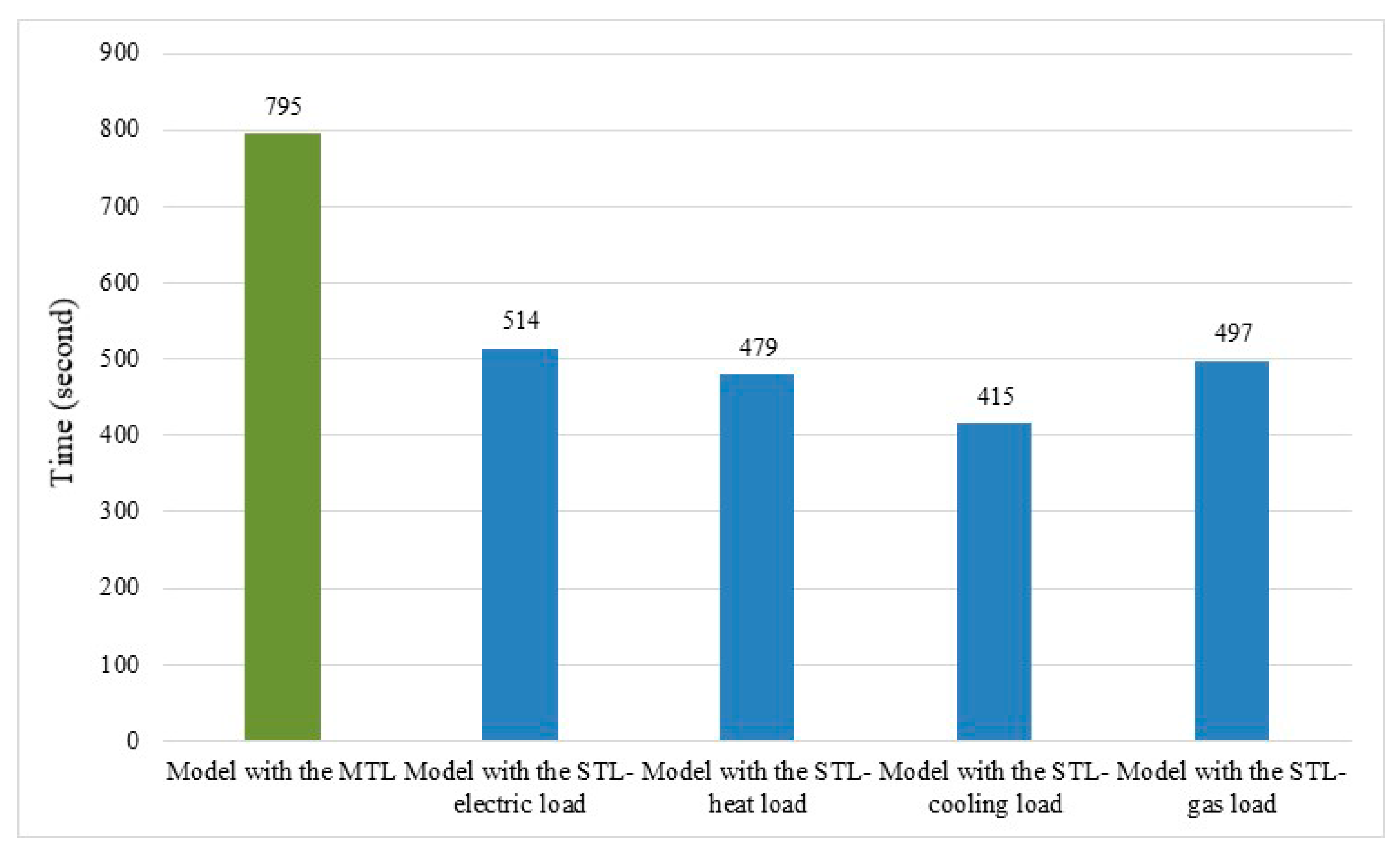
Through comparing the prediction accuracy of the Bootstrap-ISSA-MKELM based on the MTL method and the Bootstrap-ISSA-MKELM based on the STL method, it can be found that the Bootstrap-ISSA-MKELM based on the MTL method has superior performance than that based on the STL method. This is primarily because the MTL mechanism can comprehensively consider the complicated coupling relations among electric, heat, cooling, and gas loads in the IES, and make full use of the information of multi-energy loads. When one load is predicted, the information contained other related loads will be utilized, so that the prediction accuracy of electric, heat, cooling, and gas loads has been greatly improved. Additionally, the MTL mechanism can effectively shorten the calculation time. This is mainly because that the uncertain interval prediction results of the four kinds of loads can be obtained by one time via the model based on the MTL method as the multi-energy loads data can be input into the model at one time. However, the STL mechanism needs to train each energy load one by one, which makes the cumulative training time becomes longer.

(3)

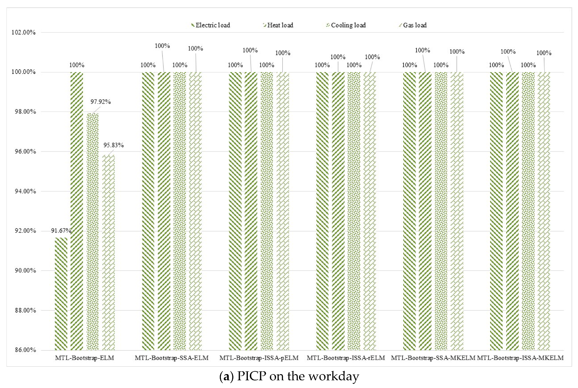
Through comparing the results of the proposed model and five comparison models (including MTL-Bootstrap-ELM, MTL-Bootstrap-SSA-ELM, MTL-Bootstrap-ISSA -pELM, MTL-Bootstrap-ISSA-rELM, and MTL-Bootstrap-SSA-MKELM), it can be found that the proposed ISSA and the MKELM method in this paper is effective and feasible in uncertain interval prediction of the combined electricity-heat-cooling-gas loads in the IES. Additionally, the established uncertain interval prediction model MTL-Bootstrap-ISSA- MKELM in this paper has the superior performance in combined electricity-heat-cooling-gas loads uncertain interval prediction than other five selected models.

References

1. Cai, W.; Liu, C.; Lai, K.-H.; Li, L.; Cunha, J.; Hu, L. Energy performance certification in mechanical manufacturing industry: A review and analysis. Energy Convers. Manag. 2019, 186, 415–432. [Google Scholar] [CrossRef]
2. Zhou, X.; Feng, C. The impact of environmental regulation on fossil energy consumption in China: Direct and indirect effects. J. Clean. Prod. 2017, 142, 3174–3183. [Google Scholar] [CrossRef]
3. Collins, S.; Deane, J.P.; Poncelet, K.; Panos, E.; Pietzcker, R.C.; Delarue, E.; Ó Gallachóir, B.P. Integrating short term variations of the power system into integrated energy system models: A methodological review. Renew. Sustain. Energy Rev. 2017, 76, 839–856. [Google Scholar] [CrossRef] [Green Version]
4. Yuan, X.-C.; Sun, X.; Zhao, W.; Mi, Z.; Wang, B.; Wei, Y.-M. Forecasting China’s ronal energy demand by 2030: A Bayesian approach. Resour. Conserv. Recycl. 2017, 127, 85–95. [Google Scholar] [CrossRef]
5. Ranaweera, D.K.; Karady, G.G.; Farmer, R.G. Economic impact analysis of load forecasting. IEEE Trans. Power Syst. 1997, 12, 1388–1392. [Google Scholar] [CrossRef]
6. Xiao, L.; Wang, J.; Yang, X.; Xiao, L. A hybrid model based on data preprocessing for electrical power forecasting. Int. J. Electr. Power Energy Syst. 2015, 64, 311–327. [Google Scholar] [CrossRef]
7. Wang, Y.; Wang, Y.; Huang, Y.; Li, F.; Zeng, M.; Li, J.; Wang, X.; Zhang, F. Planning and operation method of the ronal integrated energy system considering economy and environment. Energy 2019, 171, 731–750. [Google Scholar] [CrossRef]
8. Yang, Y.; Li, S.; Li, W.; Qu, M. Power load probability density forecasting using Gaussian process quantile regression. Appl. Energy 2018, 213, 499–509. [Google Scholar] [CrossRef]
9. Guo, Z.; Zhou, K.; Zhang, X.; Yang, S. A deep learning model for short-term power load and probability density forecasting. Energy 2018, 160, 1186–1200. [Google Scholar] [CrossRef]
10. Kim, Y.; Son, H.; Kim, S. Short term electricity load forecasting for institutional buildings. Energy Rep. 2019, 5, 1270–1280. [Google Scholar] [CrossRef]
11. Yang, A.; Li, W.; Yang, X. Short-term electricity load forecasting based on feature selection and Least Squares Support Vector Machines. Knowl. Based Syst. 2019, 163, 159–173. [Google Scholar] [CrossRef]
12. Geysen, D.; De Somer, O.; Johansson, C.; Brage, J.; Vanhoudt, D. Operational thermal load forecasting in district heating networks using machine learning and expert advice. Energy Build. 2018, 162, 144–153. [Google Scholar] [CrossRef]
13. Suryanarayana, G.; Lago, J.; Geysen, D.; Aleksiejuk, P.; Johansson, C. Thermal load forecasting in district heating networks using deep learning and advanced feature selection methods. Energy 2018, 157, 141–149. [Google Scholar] [CrossRef]
14. Nigitz, T.; Gölles, M. A generally applicable, simple and adaptive forecasting method for the short-term heat load of consumers. Appl. Energy 2019, 241, 73–81. [Google Scholar] [CrossRef]
15. Zhou, X.; Zi, X.; Liang, L.; Fan, Z.; Yan, J.; Pan, D. Forecasting performance comparison of two hybrid machine learning models for cooling load of a largescale commercial building. J. Build. Eng. 2019, 21, 64–73. [Google Scholar]
16. Ahmad, T.; Chen, H.; Shair, J.; Xu, C. Deployment of data-mining short and medium-term horizon cooling load forecasting models for building energy optimization and management. Int. J. Refrig. 2019, 98, 399–409. [Google Scholar] [CrossRef]
17. Beyca, O.F.; Ervural, B.C.; Tatoglu, E.; Ozuyar, P.G.; Zaim, S. Using machine learning tools for forecasting natural gas consumption in the province of Istanbul. Energy Econ. 2019, 80, 937–949. [Google Scholar] [CrossRef]
18. Shi, J.; Tan, T.; Guo, J.; Liu, Y. Multi-task learning based on deep architecture for various types of load forecasting in regional energy system integration. Power Syst. Technol. China 2018, 42, 698–706. [Google Scholar]
19. Tan, Z.; De, G.; Li, M.; Lin, H.; Yang, S.; Huang, L.; Tan, Q. Combined electricity-heat-cooling-gas load forecasting model for integrated energy system based on multi-task learning and least square support vector machine. J. Clean. Prod. 2020, 248, 119252. [Google Scholar] [CrossRef]
20. Lazos, D.; Sproul, A.B.; Kay, M. Optimisation of energy management in commercial buildings with weather forecasting inputs: A review. Renew. Sustain. Energy Rev. 2014, 39, 587–603. [Google Scholar] [CrossRef]
21. Nepal, B.; Yamaha, M.; Yokoe, A.; Yamaji, T. Electricity load forecasting using clustering and ARIMA model for energy management in buildings. Jpn. Archit. Rev. 2020, 3, 62–76. [Google Scholar] [CrossRef] [Green Version]
22. Amini, M.H.; Kargarian, A.; Karabasoglu, O. ARIMA-based decoupled time series forecasting of electric vehicle charging demand for stochastic power system operation. Electr. Power Syst. Res. 2016, 140, 378–390. [Google Scholar] [CrossRef]
23. Wang, Q.; Li, S.; Li, R.; Ma, M. Forecasting US shale gas monthly production using a hybrid ARIMA and metabolic nonlinear grey model. Energy 2018, 160, 378–387. [Google Scholar] [CrossRef]
24. Li, W.Q.; Chang, L. A combination model with variable weight optimization for short-term electrical load forecasting. Energy 2018, 164, 575–593. [Google Scholar] [CrossRef]
25. Amber, K.P.; Aslam, M.W.; Hussain, S.K. Electricity consumption forecasting models for administration buildings of the UK higher education sector. Energy Build. 2015, 90, 127–136. [Google Scholar] [CrossRef]
26. Capozzoli, A.; Grassi, D.; Causone, F. Estimation models of heating energy consumption in schools for local authorities planning. Energy Build. 2015, 105, 302–313. [Google Scholar] [CrossRef] [Green Version]
27. Fan, G.-F.; Peng, L.-L.; Hong, W.-C. Short term load forecasting based on phase space reconstruction algorithm and bi-square kernel regression model. Appl. Energy 2018, 224, 13–33. [Google Scholar] [CrossRef]
28. Lei, J.; Jin, T.; Hao, J.; Li, F. Short-term load forecasting with clustering–regression model in distributed cluster. Clust. Comp. 2019, 22, 10163–10173. [Google Scholar] [CrossRef]
29. Pereira, C.M.; de Almeida, N.N.; Velloso, M.L.F. Fuzzy modeling to forecast an electric load time series. Procedia Comput. Sci. 2015, 55, 395–404. [Google Scholar] [CrossRef] [Green Version]
30. Černe, G.; Dovžan, D.; Škrjanc, I. Short-term load forecasting by separating daily profiles and using a single fuzzy model across the entire domain. IEEE Trans. Ind. Electr. 2018, 65, 7406–7415. [Google Scholar] [CrossRef]
31. Coelho, V.N.; Coelho, I.M.; Coelho, B.N.; Reis, A.J.R. A self-adaptive evolutionary fuzzy model for load forecasting problems on smart grid environment. Appl. Energy 2016, 169, 567–584. [Google Scholar] [CrossRef]
32. Malekizadeh, M.; Karami, H.; Karimi, M.; Moshari, A.; Sanjari, M.J. Short-term load forecast using ensemble neuro-fuzzy model. Energy 2020, 196, 117–127. [Google Scholar] [CrossRef]
33. Xu, N.; Dang, Y.; Gong, Y. Novel grey prediction model with nonlinear optimized time response method for forecasting of electricity consumption in China. Energy 2017, 118, 473–480. [Google Scholar] [CrossRef]
34. Zhao, H.; Guo, S. An optimized grey model for annual power load forecasting. Energy 2016, 107, 272–286. [Google Scholar] [CrossRef]
35. Mi, J.; Fan, L.; Duan, X.; Qiu, Y. Short-term power load forecasting method based on improved exponential smoothing grey model. Math. Prob. Eng. 2018, 2018, 1–11. [Google Scholar] [CrossRef] [Green Version]
36. Özcan, T. Application of Seasonal and Multivariable Grey Prediction Models for Short-Term Load Forecasting. Alphanumeric J. 2017, 5, 329–338. [Google Scholar]
37. Kim, J.; Moon, J.; Hwang, E.; Kang, P. Recurrent inception convolution neural network for multi short-term load forecasting. Energy Build. 2019, 194, 328–341. [Google Scholar] [CrossRef]
38. Deng, Z.; Wang, B.; Xu, Y.; Xu, T.; Liu, C.; Zhu, Z. Multi-scale convolutional neural network with time-cognition for multi-step short-term load forecasting. IEEE Access 2019, 7, 88058–88071. [Google Scholar]
39. Zahid, M.; Ahmed, F.; Javaid, N.; Abbasi, R.A.; Kazmi, H.S.Z.; Javaid, A.; Bilal, M.; Akbar, M.; Ilahi, M. Electricity price and load forecasting using enhanced convolutional neural network and enhanced support vector regression in smart grids. Electronics 2019, 8, 122. [Google Scholar] [CrossRef] [Green Version]
40. Chen, H.; Wang, S.; Wang, S.; Li, Y. Day-ahead aggregated load forecasting based on two-terminal sparse coding and deep neural network fusion. Electr. Power Syst. Res. 2019, 177, 105987. [Google Scholar] [CrossRef]
41. Ge, Q.; Guo, C.; Jiang, H.; Lu, Z.; Yao, G.; Zhang, J.; Hua, Q. Industrial Power Load Forecasting Method Based on Reinforcement Learning and PSO-LSSVM. IEEE Trans. Cybern. 2020, 1–13. [Google Scholar]
42. Xiong, J.; Wang, T.; Li, R. Research on a hybrid LSSVM intelligent algorithm in short term load forecasting. Clust. Comp. 2019, 22, 8271–8278. [Google Scholar] [CrossRef]
43. Ma, H.; Tang, J.M. Short-Term Load Forecasting of Microgrid Based on Chaotic Particle Swarm Optimization. Procedia Comp. Sci. 2020, 166, 546–550. [Google Scholar] [CrossRef]
44. Zhang, H.; Yang, Y.; Zhang, Y.; He, Z.; Yuan, W.; Yang, Y.; Qiu, W.; Li, L. A combined model based on SSA, neural networks, and LSSVM for short-term electric load and price forecasting. Neural Comp. Appl. 2020, 33, 1–16. [Google Scholar] [CrossRef]
45. Li, S.; Goel, L.; Wang, P. An ensemble approach for short-term load forecasting by extreme learning machine. Appl. Energy 2016, 170, 22–29. [Google Scholar] [CrossRef]
46. Chen, Y.; Kloft, M.; Yang, Y.; Li, C.; Li, L. Mixed kernel based extreme learning machine for electric load forecasting. Neurocomputing 2018, 312, 90–106. [Google Scholar] [CrossRef]
47. Li, C.; Lin, S.; Xu, F.; Liu, D.; Liu, J. Short-term wind power prediction based on data mining technology and improved support vector machine method: A case study in Northwest China. J. Clean. Prod. 2018, 205, 909–922. [Google Scholar] [CrossRef]
48. Li, C.; Georgiopoulos, M.; Anagnostopoulos, G.C. Multitask classification hypothesis space with improved generalization bounds. IEEE Trans. Neural Netw. Learn. Syst. 2015, 26, 1468–1479. [Google Scholar] [CrossRef] [Green Version]
49. Li, Y.; Tian, X.; Liu, T.; Tao, D. On better exploring and exploiting task relationships in multitask learning: Joint model and feature learning. IEEE Trans. Neural Netw. Learn. Syst. 2014, 29, 1975–1985. [Google Scholar] [CrossRef] [PubMed] [Green Version]
50. Chandra, R.; Ong, Y.-S.; Goh, C.-K. Co-evolutionary multi-task learning with predictive recurrence for multi-step chaotic time series prediction. Neurocomputing 2017, 243, 21–34. [Google Scholar] [CrossRef]
51. Chandra, R.; Ong, Y.-S.; Goh, C.-K. Co-evolutionary multi-task learning for dynamic time series prediction. Appl. Soft Comput. 2018, 70, 576–589. [Google Scholar] [CrossRef] [Green Version]
52. Nunes, M.; Gerding, E.; McGroarty, F.; Niranjan, M. A comparison of multitask and single task learning with artificial neural networks for yield curve forecasting. Expert Syst. Appl. 2019, 119, 362–375. [Google Scholar] [CrossRef] [Green Version]
53. Shireen, T.; Shao, C.; Wang, H.; Li, J.; Zhang, X.; Li, M. Iterative multi-task learning for time-series modeling of solar panel PV outputs. Appl. Energy 2018, 212, 654–662. [Google Scholar] [CrossRef]
54. Xu, L.; Wang, S.; Tang, R. Probabilistic load forecasting for buildings considering weather forecasting uncertainty and uncertain peak load. Appl. Energy 2019, 237, 180–195. [Google Scholar] [CrossRef]
55. Zhu, X.; Zeng, B.; Dong, H.; Liu, J. An interval-prediction based robust optimization approach for energy-hub operation scheduling considering flexible ramping products. Energy 2020, 194, 116821. [Google Scholar] [CrossRef]
56. Khosravi, A.; Nahavandi, S.; Creighton, D.; Atiya, A.F. Lower upper bound estimation method for construction of neural network-based prediction intervals. IEEE Trans. Neural Netw. 2010, 22, 337–346. [Google Scholar] [CrossRef] [PubMed]
57. Lauret, P.; Fock, E.; Randrianarivony, R.N.; Manicom-Ramsamy, J.-F. Bayesian neural network approach to short time load forecasting. Energy Convers. Manag. 2008, 49, 1156–1166. [Google Scholar] [CrossRef]
58. Sun, M.; Zhang, T.; Wang, Y.; Strbac, G.; Kang, C. Using Bayesian deep learning to capture uncertainty for residential net load forecasting. IEEE Trans. Power Syst. 2019, 35, 188–201. [Google Scholar] [CrossRef] [Green Version]
59. He, F.; Zhou, J.; Feng, Z.-K.; Liu, G.; Yang, Y. A hybrid short-term load forecasting model based on variational mode decomposition and long short-term memory networks considering relevant factors with Bayesian optimization algorithm. Appl. Energy 2019, 237, 103–116. [Google Scholar] [CrossRef]
60. Yang, Y.; Li, W.; Gulliver, T.A.; Li, S. Bayesian Deep Learning-Based Probabilistic Load Forecasting in Smart Grids. IEEE Trans. Ind. Inf. 2019, 16, 4703–4713. [Google Scholar] [CrossRef]
61. Zhang, J.; Wang, Y.; Sun, M.; Zhang, N. Two-Stage Bootstrap Sampling for Probabilistic Load Forecasting. IEEE Trans. Eng. Manag. 2020, 1–9. [Google Scholar] [CrossRef]
62. Xu, Y.; Mi, C.; Zhu, Q.-X.; Gao, J.-Y.; He, Y.-L. An effective high-quality prediction intervals construction method based on parallel bootstrapped RVM for complex chemical processes. Chemom. Int. Lab. Syst. 2017, 171, 161–169. [Google Scholar] [CrossRef]
63. Liu, Z.F.; Li, L.L.; Tseng, M.L.; Lim, M.K. Prediction short-term photovoltaic power using improved chicken swarm optimizer-Extreme learning machine model. J. Clean. Prod. 2020, 248, 119272. [Google Scholar] [CrossRef]
64. Chen, H.; Zhang, Q.; Luo, J.; Xu, Y.; Zhang, X. An enhanced Bacterial Foraging Optimization and its application for training kernel extreme learning machine. Appl. Soft Comp. 2020, 86, 105884. [Google Scholar] [CrossRef]
65. Liu, X.; Wang, L.; Huang, G.-B.; Zhang, J.; Yin, J. Multiple kernel extreme learning machine. Neurocomputing 2015, 149, 253–264. [Google Scholar] [CrossRef]
66. Wang, M.; Chen, H.; Li, H.; Cai, Z.; Zhao, X.; Tong, C.; Li, J.; Xu, X. Grey wolf optimization evolving kernel extreme learning machine: Application to bankruptcy prediction. Eng. Appl. Art. Int. 2017, 63, 54–68. [Google Scholar] [CrossRef]
67. Evgeniou, T.; Charles, A.M.; Massimiliano, P. Learning multiple tasks with kernel methods. J. Mach. Learn. Res. 2005, 6, 615–637. [Google Scholar]
68. Xu, S.; An, X.; Qiao, X.; Zhu, L.; Li, L. Multi-output least-squares support vector regression machines. Pattern Recognit. Lett. 2013, 34, 1078–1084. [Google Scholar] [CrossRef]
69. Bădin, L.; Cinzia, D.; Léopold, S. A bootstrap approach for bandwidth selection in estimating conditional efficiency measures. Eur. J. Oper. Res. 2019, 277, 784–797. [Google Scholar] [CrossRef]
70. Flores-Agreda, D.; Cantoni, E. Bootstrap estimation of uncertainty in prediction for generalized linear mixed models. Comp. Stat. Data Anal. 2019, 130, 1–17. [Google Scholar] [CrossRef] [Green Version]
71. Li, K.; Wang, R.; Lei, H.; Zhang, T.; Liu, Y.; Zheng, X. Interval prediction of solar power using an Improved Bootstrap method. Sol. Energy 2018, 159, 97–112. [Google Scholar] [CrossRef]
72. Huang, G.B.; Zhou, H.; Ding, X.; Zhang, R. Extreme learning machine for regression and multiclass classification. IEEE Trans. Syst. Man Cybern. Part B (Cybern.) 2011, 42, 513–529. [Google Scholar] [CrossRef] [Green Version]
73. Zhang, Y.; Wang, Y.; Zhou, G.; Jin, J.; Wang, B.; Wang, X.; Cichocki, A. Multi-kernel extreme learning machine for EEG classification in brain-computer interfaces. Expert Syst. Appl. 2018, 96, 302–310. [Google Scholar] [CrossRef]
74. Liu, Z.; Loo, C.K.; Pasupa, K. A novel error-output recurrent two-layer extreme learning machine for multi-step time series prediction. Sustain. Cities Soc. 2021, 66, 102613. [Google Scholar] [CrossRef]
75. Sin, M.C.; Gan, S.N.; Annuar, M.S.M.; Tan, I.K.P. Chain cleavage mechanism of palm kernel oil derived medium-chain-length poly(3-hydroxyalkanoates) during high temperature decomposition. Polym. Degrad. Stab. 2011, 96, 1705–1710. [Google Scholar]
76. Li, Q.; Xiong, Q.; Ji, S.; Yu, Y.; Wu, C.; Yi, H. A method for mixed data classification base on RBF-ELM network. Neurocomputing 2021, 431, 7–22. [Google Scholar] [CrossRef]
77. Mirjalili, S.; Gandomi, A.H.; Mirjalili, S.Z.; Saremi, S.; Faris, H.; Mirjalili, S.M. Salp Swarm Algorithm: A bio-inspired optimizer for engineering design problems. Adv. Eng. Softw. 2017, 114, 163–191. [Google Scholar] [CrossRef]
Figure 1. The basic energy flow in the IES.
Mathematics 09 01645 g001
Figure 2. The information sharing mechanism of the MTL method.
Mathematics 09 01645 g002
Figure 3. The structure of the ELM.
Mathematics 09 01645 g003
Figure 4. The data distribution characteristics of the RBF kernel function.
Mathematics 09 01645 g004
Figure 5. The data distribution characteristics of the Poly kernel function.
Mathematics 09 01645 g005
Figure 6. Single salp (a) and salp chain (b).
Mathematics 09 01645 g006
Figure 7. The role of each method contained in the uncertain interval forecasting model for the electricity-heat-cooling-gas loads on the demand side in the IES.
Mathematics 09 01645 g007
Figure 8. The calculation process of the established uncertain interval forecasting model.
Mathematics 09 01645 g008
Figure 9. The specific input variables of the uncertain interval prediction model for multi-energy loads.
Mathematics 09 01645 g009
Figure 10. The convergence trend of the ISSA and the basic SSA.
Mathematics 09 01645 g010
Figure 11. Multi-energy load forecasting results on the workday (MW).
Mathematics 09 01645 g011aMathematics 09 01645 g011b
Figure 12. Multi-energy load forecasting results on the holiday (MW).
Mathematics 09 01645 g012
Figure 13. Multi-energy load forecast results on the workday based on the STL method.
Mathematics 09 01645 g013
Figure 14. Multi-energy load forecast results on the holiday based on the STL method.
Mathematics 09 01645 g014aMathematics 09 01645 g014b
Figure 15. Comparison of calculation time of different learning mechanisms.
Mathematics 09 01645 g015
Figure 16. Comparison of PICP and PINAW values of six prediction models.
Mathematics 09 01645 g016aMathematics 09 01645 g016bMathematics 09 01645 g016c