
Prediction of Mechanical Properties of the Stirrup-Confined Rectangular CFST Stub Columns Using FEM and Machine Learning


Abstract
:1. Introduction
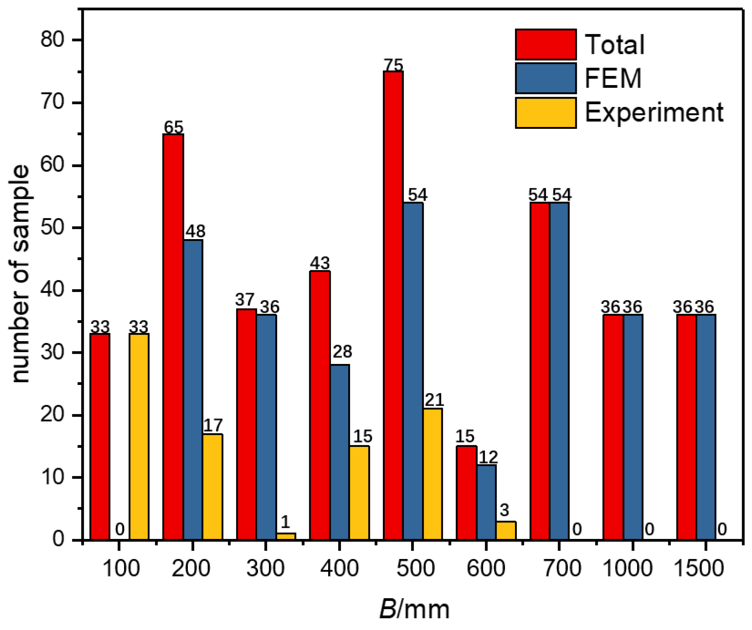
2. Experimental Data Set
3. FEM Model
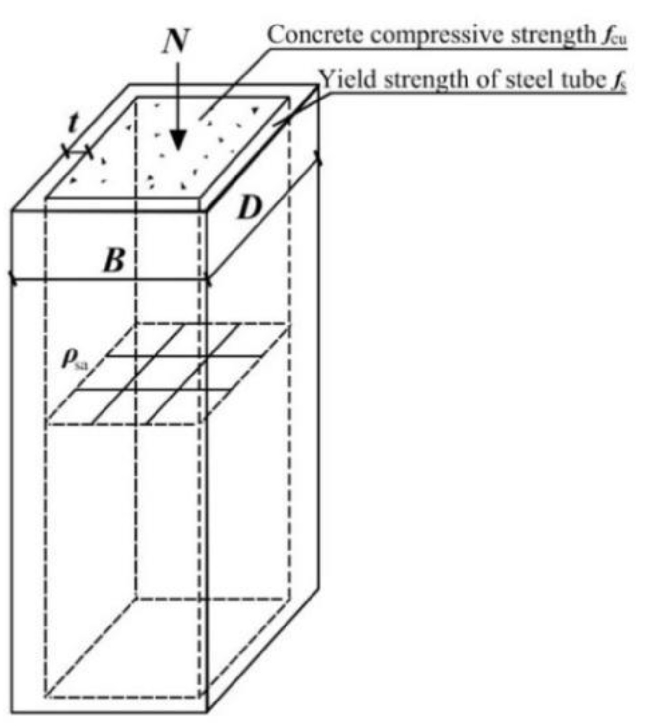
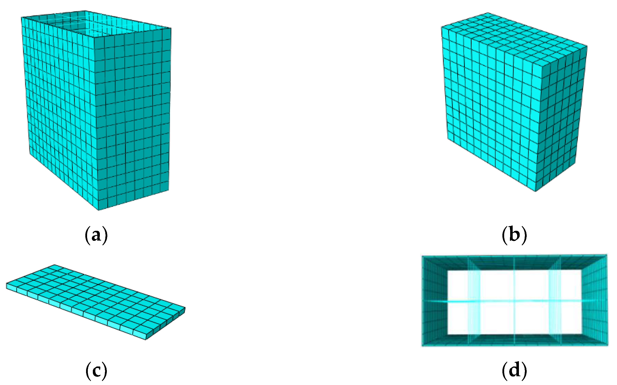
3.1. FEM Model
3.2. Parameter Setting of Finite Element Analysis
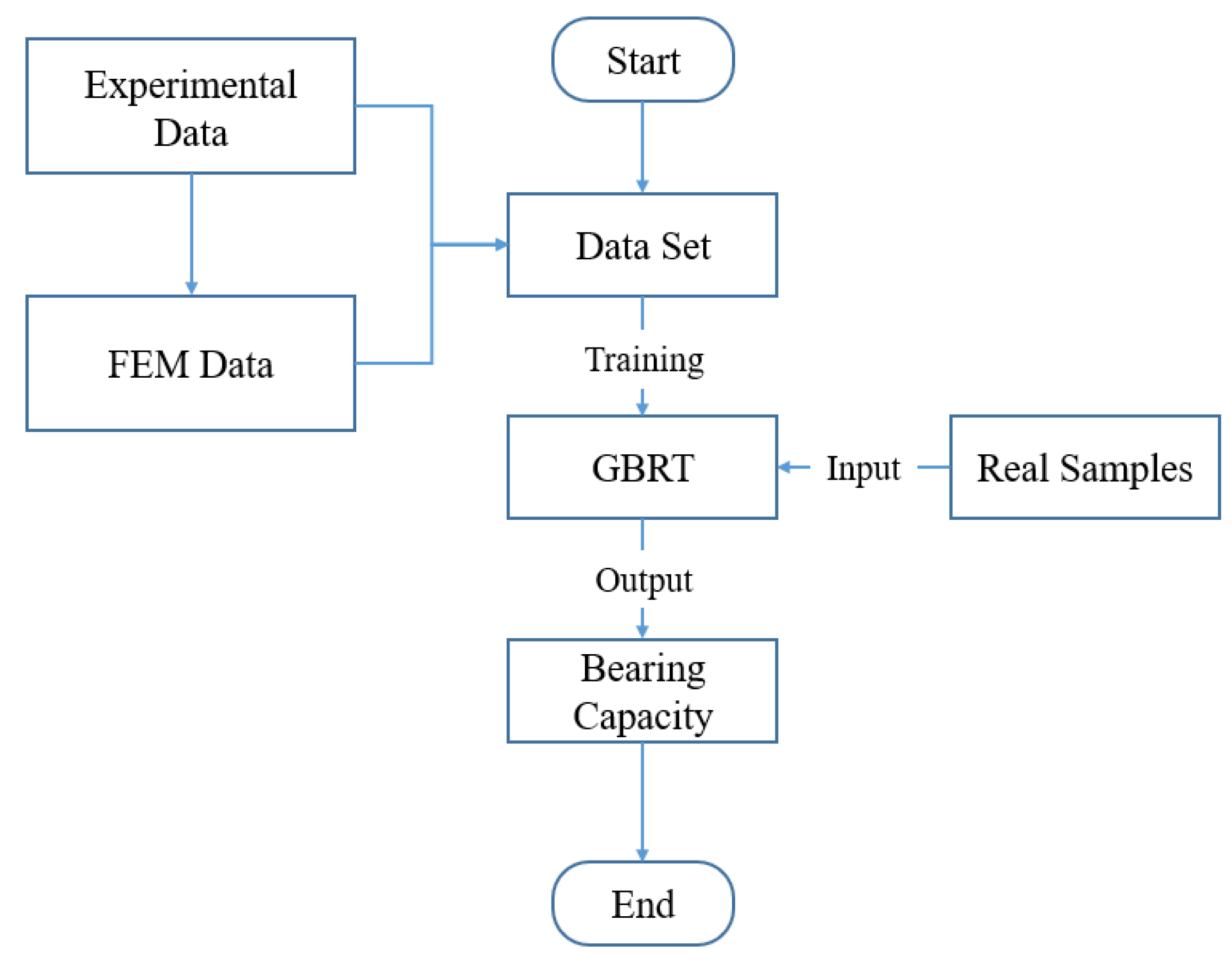
4. Property Prediction Based on Gradient Boosting Regression
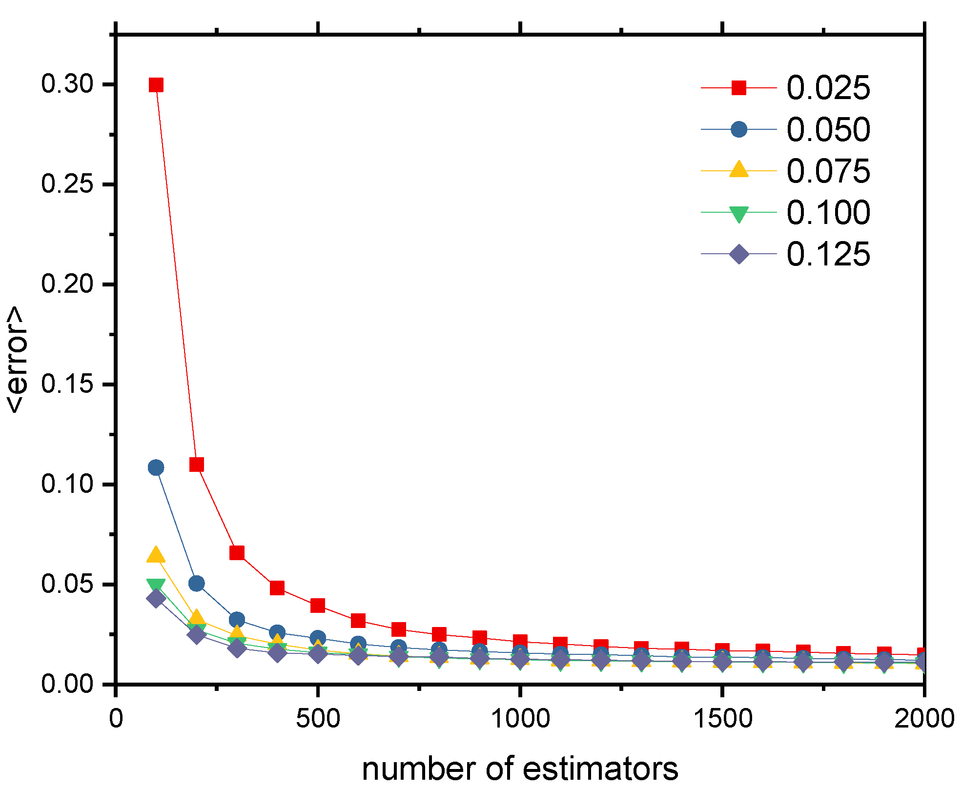
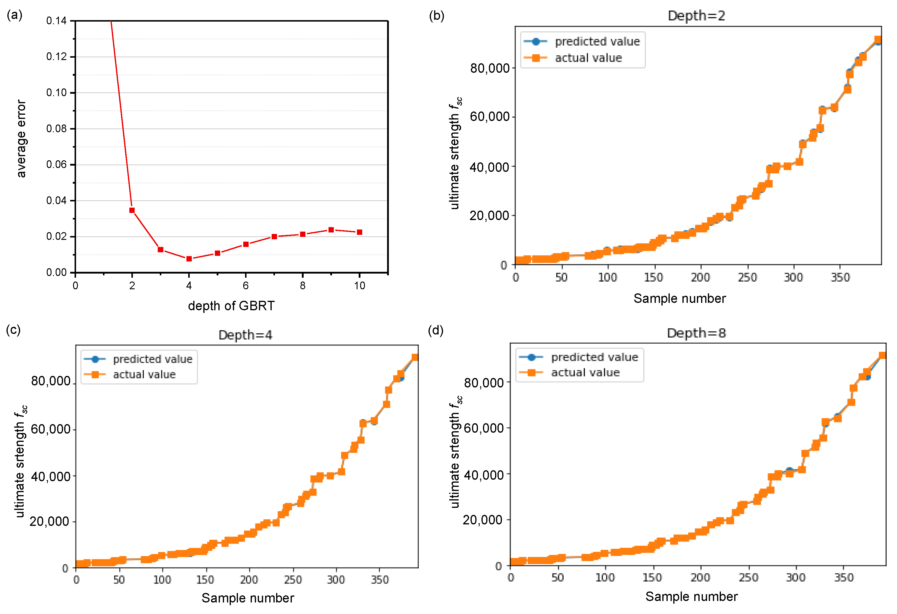
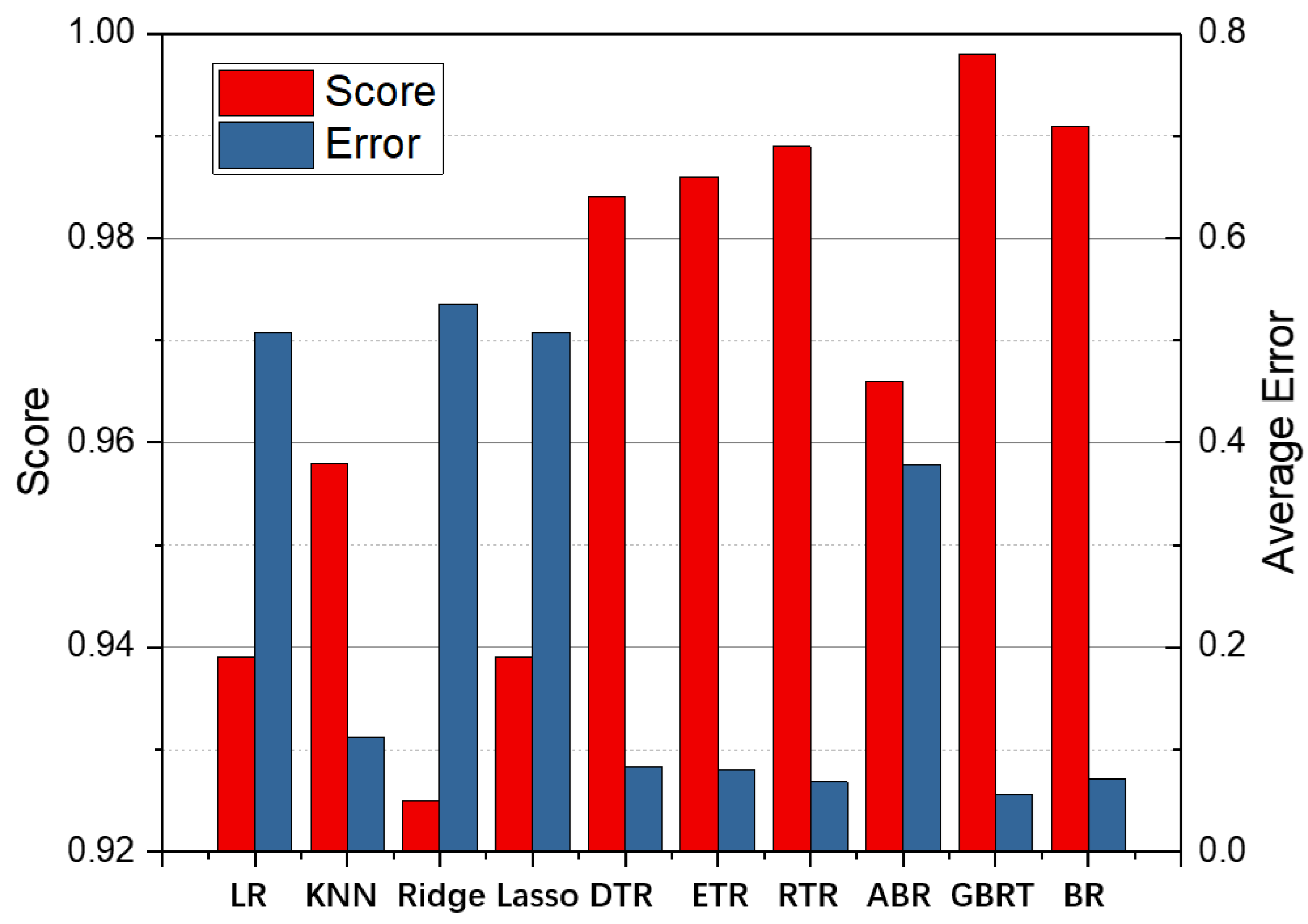
4.1. The Model Selection
| Algorithm 1 Gradient Boost |
|
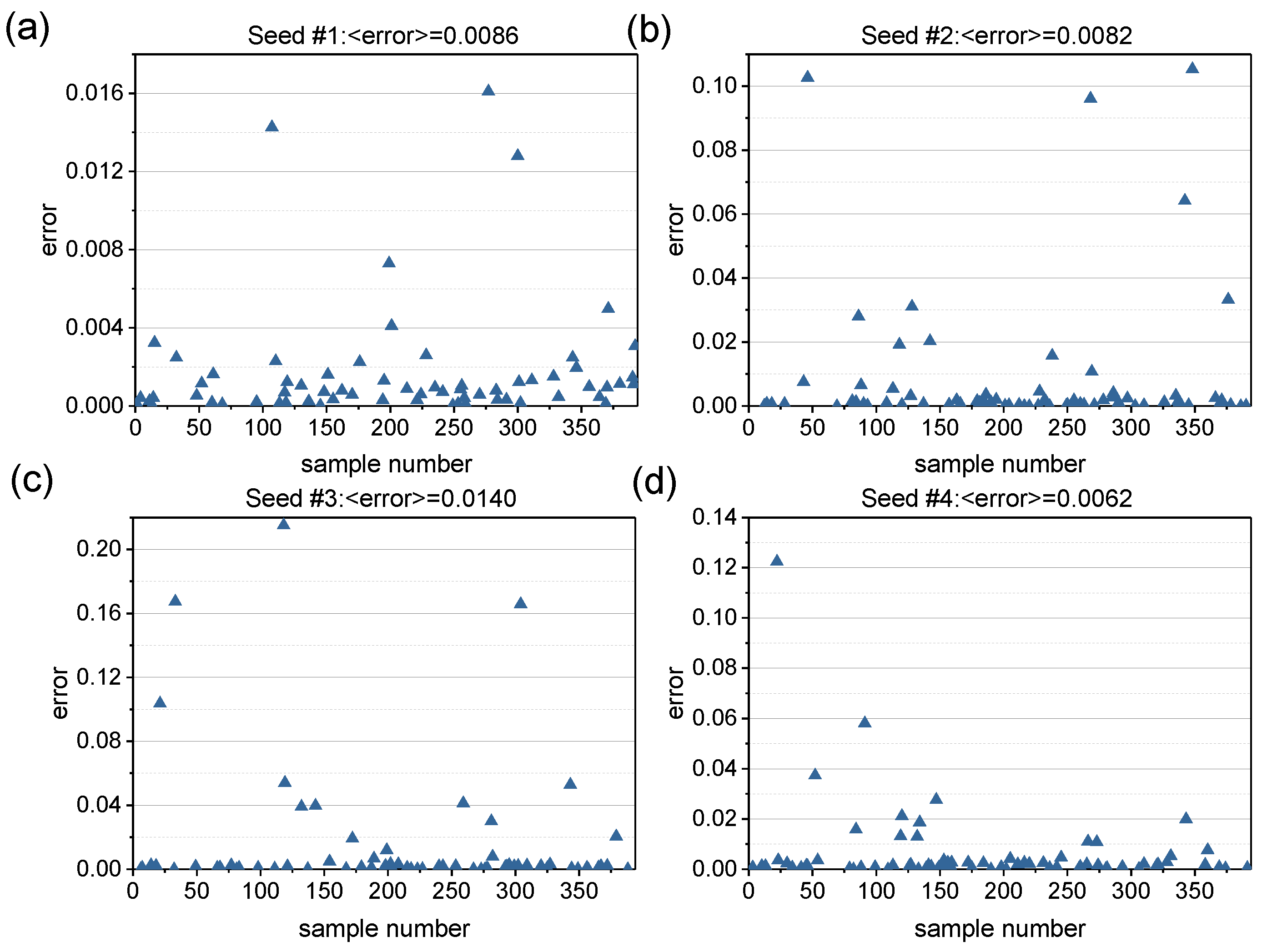
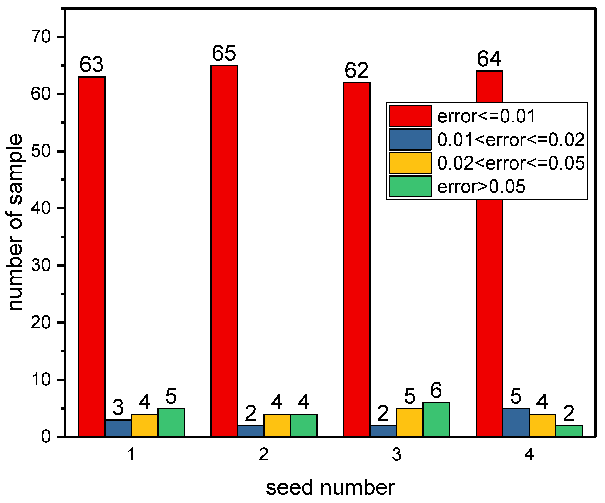
4.2. Discussion
5. Conclusions
Author Contributions
Funding
Conflicts of Interest
References
- Han, L.H.; Li, W.; Bjorhovde, R.J. Developments and advanced applications of concrete-filled steel tubular (CFST) structures: Members. J. Constr. Steel Res. 2014, 100, 211–228. [Google Scholar] [CrossRef]
- Ding, F.-X.; Wang, W.; Liu, X.-M.; Wang, L.; Yi, S. Mechanical behavior of outer square inner circular concrete-filled dual steel tubular stub columns. Steel Compos. Struct. 2021, 38, 305–317. [Google Scholar] [CrossRef]
- Ding, F.X.; Lu, D.R.; Bai, Y.; Zhou, Q.S.; Ni, M.; Yu, Z.W.; Jiang, G.S. Comparative study of square stirrup-confined concrete-filled steel tubular stub columns under axial loading. Thin-Walled Struct. 2016, 98, 443–453. [Google Scholar] [CrossRef]
- Lu, D.R.; Wang, W.J.; Ding, F.; Liu, X.M.; Fang, C.J.J.S. The impact of stirrups on the composite action of concrete-filled steel tubular stub columns under axial loading. Structures 2021, 30, 786–802. [Google Scholar] [CrossRef]
- Samarakkody, D.I.; Thambiratnam, D.P.; Chan, T.; Moragaspitiya, P.J.C.; Materials, B. Differential axial shortening and its effects in high rise buildings with composite concrete filled tube columns. Constr. Build. Mater. 2017, 143, 659–672. [Google Scholar] [CrossRef]
- Cheng, M.Y.; Prayogo, D.; Wu, Y.W.J. Novel Genetic Algorithm-Based Evolutionary Support Vector Machine for Optimizing High-Performance Concrete Mixture. J. Comput. Civ. Eng. 2013, 28, 06014003. [Google Scholar] [CrossRef] [Green Version]
- Bui, D.T.; Nhu, V.H.; Hoang, N.D. Prediction of soil compression coefficient for urban housing project using novel integration machine learning approach of swarm intelligence and Multi-layer Perceptron Neural Network. Adv. Eng. Inform. 2018, 38, 593–604. [Google Scholar]
- Hoang, N.D.; Bui, D.T. Predicting earthquake-induced soil liquefaction based on a hybridization of kernel Fisher discriminant analysis and a least squares support vector machine: A multi-dataset study. Bull. Eng. Geol. Environ. 2018, 77, 191–204. [Google Scholar] [CrossRef]
- Moosazadeh, S.; Namazi, E.; Aghababaei, H.; Marto, A.; Mohamad, H.; Hajihassani, M. Prediction of building damage induced by tunnelling through an optimized artificial neural network. Eng. Comput. 2019, 35, 579–591. [Google Scholar] [CrossRef]
- Sharma, L.K.; Singh, T.N. Regression-based models for the prediction of unconfined compressive strength of artificially structured soil. Eng. Comput. 2017. [Google Scholar] [CrossRef]
- Rafiei, M.H.; Khushefati, W.H.; Demirboga, R.; Adeli, H.J.A.M.J. Supervised Deep Restricted Boltzmann Machine for Estimation of Concrete. Aci. Mater. J. 2017, 114, 237–244. [Google Scholar] [CrossRef]
- Sarveghadi, M.; Gandomi, A.H.; Bolandi, H.; Alavi, A.H. Development of prediction models for shear strength of SFRCB using a machine learning approach. Neural Comput. Appl. 2015, 1–10. [Google Scholar] [CrossRef]
- Nilsen, V.; Pham, L.T.; Hibbard, M.; Klager, A.; Cramer, S.M.; Morgan, D.J.C.; Materials, B. Prediction of concrete coefficient of thermal expansion and other properties using machine learning. Constr. Build. Mater. 2019, 220, 587–595. [Google Scholar] [CrossRef]
- Prayogo, D.; Cheng, M.-Y.; Wu, Y.-W.; Tran, D.-H. Combining machine learning models via adaptive ensemble weighting for prediction of shear capacity of reinforced-concrete deep beams. Eng. Comput. 2020, 36, 1135–1153. [Google Scholar] [CrossRef]
- Ding, F.-X.; Luo, L.; Zhu, J.; Wang, L.; Yu, Z.-W. Mechanical behavior of stirrup-confined rectangular CFT stub columns under axial compression. Thin-Walled Struct. 2018, 124, 136–150. [Google Scholar] [CrossRef]
- Chen, Z.H.; Du, Y.S.; Wu, L.; Qin, Y.; Zhou, T. Summary of research on concrete filled rectangular steel tube structure. Build. Struct. 2015. (In Chinese) [Google Scholar] [CrossRef]
- Rao, Y.L.; Zhang, J.C.; Li, Y.; Huang, Y.B.; Li, D. Test of bearing capacity of concrete filled rectangular steel tubular stub columns under axial compression. J. Huaqiao Univ. (Nat. Sci.) 2019, 40, 338–343. (In Chinese) [Google Scholar]
- Qu, X.S.; Liu, Q. Study on the axial compression behavior of concrete-filled rectangular steel tubular columns. Build. Sci. 2018, 34, 37–42. (In Chinese) [Google Scholar]
- Jing, S.Y.; Zheng, X.Q.; Zhu, J.S. Research on the mechanical behavior of the square thick-walled concrete-filled steel tube short column. Ind. Constr. 1989, 11, 8–13. (In Chinese) [Google Scholar]
- Hu, H.T.; Huang, C.S.; Wu, M.H.; Wu, Y.M. Nonlinear analysis of axially loaded concrete-filled tube columns with confinement effect. J. Struct. Eng. 2003, 129, 1322–1329. [Google Scholar] [CrossRef]
- Baltay, P.; Gjelsvik, A.J. Coefficient of Friction for Steel on Concrete at High Normal Stress. J. Mater. Civ. Eng. 1990, 2, 46–49. [Google Scholar] [CrossRef]
- Yu, Z.-W.; Ding, F.X.; Cai, C.S. Experimental behavior of circular concrete-filled steel tube stub columns. J. Constr. Steel Res. 2007, 63, 165–174. [Google Scholar] [CrossRef]
- Ottosen, N.S.; Ristinmaa, M. Common Plasticity Models. Mech. Const. Model. 2005, 279–319. [Google Scholar] [CrossRef]
- Ding, F.; Ying, X.; Zhou, L.; Yu, Z.; China, C.E. Unified calculation method and its application in determining the uniaxial mechanical properties of concrete. Front. Archit. Civ. Eng. China 2011, 5, 381–393. [Google Scholar] [CrossRef]
- Harper, Angel, Inc. ABAQUS User’s Manuals; Version 6.9; Simulia, Providence: Johnston, RI, USA, 2009. [Google Scholar]
- Ding, F.; Zhu, J.; Cheng, S.; Liu, X. Comparative study of stirrup-confined circular concrete-filled steel tubular stub columns under axial loading. Thin-Walled Struct. 2018, 123, 294–304. [Google Scholar] [CrossRef] [Green Version]
- Pedregosa, F.; Varoquaux, G.; Gramfort, A.; Michel, V.; Thirion, B.; Grisel, O.; Blondel, M.; Müller, A.; Nothman, J.; Louppe, G. Scikit-learn: Machine Learning in Python. J. Mach. Learn. Res. 2011, 12, 2825–2830. [Google Scholar]
- Friedman, J. Greedy function approximation: A gradient boosting machine. Ann. Stat. 2001, 29, 1189–1232. [Google Scholar] [CrossRef]
- Kriegler, B.; Berk, R. Stochastic Gradient Boosting. Comput. Stat. Data Anal. 2010, 38, 367–378. [Google Scholar]
- Friedman, J.; Hastie, T.; Tibshirani, R. Additive logistic regression: A statistical view of boosting (with discussion and a rejoinder by the authors). Ann. Stat. 2000, 28, 337–374. [Google Scholar] [CrossRef]
- Freund, Y.J. Experiments with a new boosting algorithm. icml Citeseer 1996, 148–156. Available online: https://www.researchgate.ne-t/Publication/244498683_Experiment_With_a_New_Boosting_Algorithm (accessed on 10 June 2021).
- Björck, Å. Numerical Methods for Least Squares Problems. SIAM 1996. [Google Scholar] [CrossRef]
- Sun, H.; Xu, Q.; Yan, P.; Yin, J.; Lou, P. A Study on Axial Compression Performance of Concrete-Filled Steel-Tubular Shear Wall with a Multi-Cavity T-Shaped Cross-Section. Energies 2020, 13, 4831. [Google Scholar] [CrossRef]


| Aspect Ratio | B/D = 1 | B/D = 1.5 | B/D = 2 | B/D = 3 |
|---|---|---|---|---|
| RST |  |  |  |  |
| SST |  |  |  |  |
| Variables | Unit | Min | Max | Mean |
|---|---|---|---|---|
| X1 = section length (B) | mm | 121 | 601 | 266.3 |
| X2 = section width (D) | mm | 100 | 300 | 188.1 |
| X3 = steel tube thickness (t) | mm | 2 | 7.36 | 4.57 |
| X4 = equivalent stirrup ratio(ρsa) | % | 0 | 1.1 | 0.2 |
| X5 = concrete compressive strength (fcu) | MPa | 23.8 | 70.8 | 40.3 |
| X6 = yield strength of steel tube(fs) | MPa | 235 | 750 | 360.9 |
| Y = ultimate bearing capacity of CFST columns (N) | KN | 1000 | 8456 | 3477.8 |
| No | B × D × t/mm | B/D | ρsa | fcu/MPa | fs/MPa | Nu,fe/kN |
|---|---|---|---|---|---|---|
| 1 | 500 × 500 × 5 | 1 | 0 | 60 | 345 | 16,241.7 |
| 2 | 500 × 500 × 5 | 1 | 0.005 | 40 | 235 | 12,006.1 |
| 3 | 750 × 500 × 6 | 1.5 | 0 | 60 | 420 | 25,516.3 |
| 4 | 750 × 500 × 6 | 1.5 | 0.015 | 60 | 235 | 26,049.7 |
| 5 | 1000 × 500 × 7 | 2 | 0 | 80 | 345 | 41,876 |
| 6 | 1000 × 500 × 7 | 2 | 0.01 | 40 | 345 | 28,674.6 |
| 7 | 1500 × 500 × 7.5 | 3 | 0 | 100 | 345 | 76,863.2 |
| 8 | 1500 × 500 × 7.5 | 3 | 0.007 | 40 | 235 | 35,168.5 |
| 9 | 500 × 250 × 4 | 2 | 0 | 38 | 323 | 6367.6 |
| 10 | 500 × 250 × 4 | 2 | 0.006 | 43 | 314 | 7637.58 |
| 11 | 375 × 250 × 3 | 1.5 | 0 | 48 | 354 | 5853.86 |
| 12 | 375 × 250 × 3 | 1.5 | 0.004 | 58 | 374 | 7268.44 |
| 13 | 400 × 200 × 4 | 2 | 0 | 63 | 382 | 6607.28 |
| 14 | 400 × 200 × 4 | 2 | 0.005 | 53 | 356 | 6220.35 |
| Seed#1 | Seed#2 | Seed#3 | Seed#4 | ||||||||
|---|---|---|---|---|---|---|---|---|---|---|---|
| 4443 | 4721 | 0.063 | 5765 | 6425 | 0.103 | 3513 | 3513 | 0.104 | 3250 | 2852 | 0.122 |
| 2516 | 2651 | 0.053 | 9910 | 9041 | 0.096 | 3450 | 4027 | 0.167 | 6572 | 6190 | 0.058 |
| 3750 | 3944 | 0.051 | 2708 | 2345 | 0.064 | 2910 | 2284 | 0.215 | |||
| 3470 | 4045 | 0.166 | 9103 | 8236 | 0.105 | 2318 | 2193 | 0.054 | |||
| 2920 | 2687 | 0.080 | 1917 | 2236 | 0.166 | ||||||
| 11,085 | 11,673 | 0.053 | |||||||||
Publisher’s Note: MDPI stays neutral with regard to jurisdictional claims in published maps and institutional affiliations. |
© 2021 by the authors. Licensee MDPI, Basel, Switzerland. This article is an open access article distributed under the terms and conditions of the Creative Commons Attribution (CC BY) license (https://creativecommons.org/licenses/by/4.0/).
Share and Cite
Lu, D.; Chen, Z.; Ding, F.; Chen, Z.; Sun, P. Prediction of Mechanical Properties of the Stirrup-Confined Rectangular CFST Stub Columns Using FEM and Machine Learning. Mathematics 2021, 9, 1643. https://doi.org/10.3390/math9141643
Lu D, Chen Z, Ding F, Chen Z, Sun P. Prediction of Mechanical Properties of the Stirrup-Confined Rectangular CFST Stub Columns Using FEM and Machine Learning. Mathematics. 2021; 9(14):1643. https://doi.org/10.3390/math9141643
Chicago/Turabian StyleLu, Deren, Zhidong Chen, Faxing Ding, Zhenming Chen, and Peng Sun. 2021. "Prediction of Mechanical Properties of the Stirrup-Confined Rectangular CFST Stub Columns Using FEM and Machine Learning" Mathematics 9, no. 14: 1643. https://doi.org/10.3390/math9141643
APA StyleLu, D., Chen, Z., Ding, F., Chen, Z., & Sun, P. (2021). Prediction of Mechanical Properties of the Stirrup-Confined Rectangular CFST Stub Columns Using FEM and Machine Learning. Mathematics, 9(14), 1643. https://doi.org/10.3390/math9141643