Simulated Annealing with Restart Strategy for the Path Cover Problem with Time Windows

Abstract

This research presents a variant of the vehicle routing problem known as the path cover problem with time windows (PCPTW), in which each vehicle starts with a particular customer and finishes its route at another customer. The vehicles serve each customer within the customer’s time windows. PCPTW is motivated by a practical strategy for companies to reduce operational cost by hiring freelance workers, thus allowing workers to directly service customers without reporting to the office. A mathematical programming model is formulated for the problem. This research also proposes a simulated annealing heuristic with restart strategy (SARS) to solve PCPTW and test it on several benchmark datasets. Computational results indicate that the proposed SARS effectively solves PCPTW.

1. Introduction

The vehicle routing problem (VRP) is widely used to address logistics and transportation problems, and on the basis of the literature over the last few decades many variants of it have been extensively studied. Examples include VRP with time windows [1,2,3,4], VRP with stochastic demand [5,6,7], time-dependent VRP [8,9,10], and VRP with split delivery [11,12,13]. Most of these studies are devoted to dealing concerns about vehicle routes in a logistics and transportation system, the resources of which belong permanently to the companies. However, in real-life situations, resources are commonly not owned permanently by companies, and this situation must be considered by decision makers.

The present work is motivated by the practical strategy currently adopted by many several small- and medium-sized enterprises (SMEs) that hire freelance workers to reduce operational costs. This practice allows workers to start driving from either their homes or certain geographical locations and return directly to them without reporting to the main office. The freelance workers can be private car owners or occasional drivers provided by delivery service companies such as Uber and Grab. Hence, hiring freelance workers provides vehicle fleet operators or companies with flexibility in planning service routes. By using this strategy, companies can assign efficient paths that disregard the distance between workers’ homes and the depot. Companies will only be concerned with the path of workers from the first to the last customer. This situation is observed in intermediate service companies (e.g., home care service providers and health home care service agencies) without resources (e.g., freelance carriers, housekeeping services, handymen, and shopping assistants), and in companies that hire freelance sales agents.

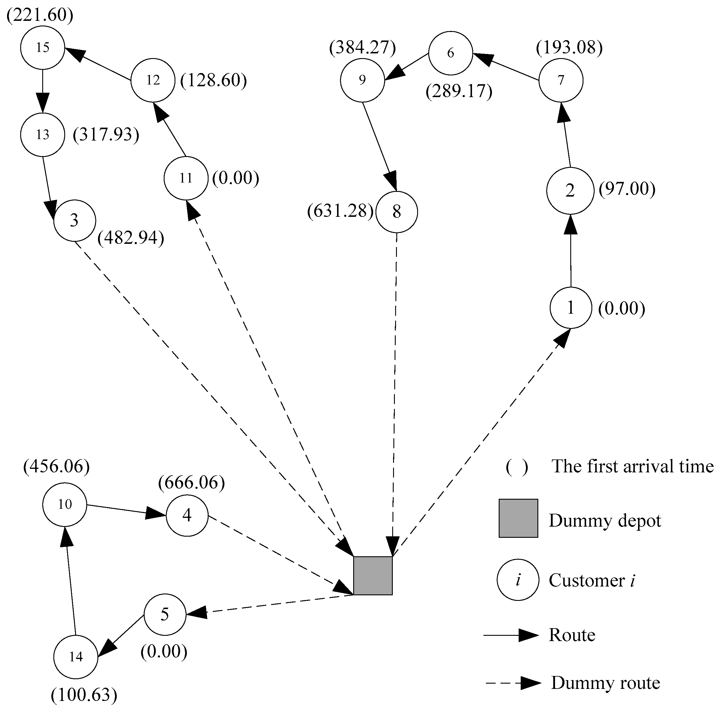
The practical strategy above creates a variant of VRP called the path cover problem (PCP) [14]. In practice, many customers want to be served within a particular time range, and thus this research extends PCP by considering time windows to propose the path cover problem with time windows (PCPTW). Figure 1 depicts an illustration of PCPTW, whose structure is similar to PCP, but also covers the service time windows of customers. As shown in Figure 1, a dummy depot and a dummy route disregard the distance from the depot to the customer.

The vehicle routing problems that consider the hiring of outsourced vehicles are commonly modeled as open vehicle routing problems (OVRPs), as presented by Salari et al. [15]. Outsourced vehicles provided by third-party logistics operators are hired to fulfill customer demands. When each customer is restricted to an earliest and latest visit time, the problem is extended to the ‘open vehicle routing problem with time windows’ (OVRPTW), as discussed in Repoussis et al. [16]. After finishing the tasks, the outsourced vehicles do not return to the depot, since they belong to third-party logistics operators. PCPTW is different from OVRP and OVRPTW in that the drivers are allowed to visit their first customer directly from their homes instead of from the main office. In practice, each route is assigned to a driver who can visit the customers within their respective time windows. This is similar to the underlying assumption of VRPTW that each driver is available to start the route at a time that allows her/him to meet the customers’ time window restrictions, including that of the first customer.

VRP is an NP-hard combinatorial optimization problem, and hence PCPTW is also an NP-hard problem. To address it, this work proposes a simulated annealing with restart strategy (SARS) heuristic, which is a diversified version of simulated annealing (SA) that utilizes a restart strategy to escape from local optima. This study conducts extensive computational experiments on a PCP dataset, well-known VRPTW benchmark problems, and a PCPTW dataset to investigate the performance of the proposed method on the three problems.

The four main contributions of this study are as follows. First, it considers time windows for PCP, which is closer to real-life situations. In addition, PCPTW is different from VRPTW [17], because it considers the open-ended paths of vehicles instead of the closed vehicle loops in VRPTW. Second, the proposed SARS is compared with an exact solver on the PCPTW dataset, which is adapted from Solomon’s VRPTW dataset. SARS obtains optimal solutions for all the small instances and can improve the upper bounds for medium and large instances. This research also investigates the advantage of the restart strategy in improving SA. Third, this work evaluates the proposed SARS’s performance against other heuristics on Solomon’s VRPTW and PCP datasets, finding that the algorithm performs at par with other heuristics. This research further compares it with another single-based solution heuristic and finds that SARS performs more efficiently. Fourth, the proposed SARS obtains new best-known solutions for six instances in Solomon’s VRPTW dataset.

The remainder of this paper is structured as follows. Section 2 presents the literature review. Section 3 presents a mathematical model for PCPTW. Section 4 discusses the proposed SARS for PCPTW. Section 5 discusses the computational study. Section 6 concludes the paper.

2. Literature Review

To the best of our knowledge, the literature has no articles devoted to PCPTW. While OVRP, OVRPTW and VRPTW are variants of VRP that are close to PCPTW, PCPTW extends PCP toward real-life aspects by considering a range of service times at the customer location. In PCP, a vehicle starts at a customer and ends at another customer without visiting the depot. This problem is introduced by Yu et al. [14] and motivated by a practical strategy of employing private vehicles to undertake the transportation function of a company or organization. In OVRP, vehicles start from the depot and terminate at a customer location, and thus there is no transportation cost associated with the distance between the last customer and the depot. This variant was first introduced by Sariklis and Powell [18] as a practical technique for companies that require delivery operations from distribution companies, called freelance vehicles, which deliver goods to customers, but are not owned by the distribution companies. In contrast to OVRP, in PCPTW there is both no distance cost between the last customer and the depot, and no distance cost between the depot and the first customer. In addition, PCPTW also ensures that vehicles serve customers in a certain time range, which is not considered in OVRP. Due to the more complex characteristics of PCPTW, solving PCPTW needs more effort compared to solving OVRP. Classical heuristic methods such as the Clarke and Wright algorithm [19], petal algorithm [20], and sweep algorithm [21] are the early solution approaches for VRP and it variants [22]. In the last few decades, metaheuristics has gained much interest from VRP researchers due to their ability to solve VRP related problems compared to the classical heuristics [23].

Many OVRP studies consider additional characteristics in real-world applications, including OVRPTW. Xia and Fu [24] proposed a variant of OVRP by considering split deliveries and solved the problem using an adaptive tabu search. The algorithm was tested on instances with up to 100 customers. Xia and Fu [25] considered time window and satisfaction rate in OVRPTW. They developed an improved tabu search algorithm for the problem. The algorithm was tested on Solomon benchmark instances with 100 customers. Lalla-Ruiz and Mes [26] presented a two-index-based mathematical formulation to solve the multi-depot OVRP. The model was tested on instances with 48 to 288 customers.

In VRPTW, vehicles start from the depot, serve all customers without violating the vehicle capacity and constraints of the customer time range, and then return to the depot. Solomon [3] solved VRPTW using sequential and parallel methods. Sequential procedures construct one route at a time until all customers are scheduled. Parallel procedures are characterized by the simultaneous construction of a number of routes. The author generated six sets of problems, which are well-known as Solomon’s VRPTW dataset. This dataset serves as a reference to subsequent researchers for testing their approaches to solving VRPTW efficiently. Thereafter, several researchers have presented metaheuristic methods as strong tools for solving VRPTW. This section underlines the methods from recently published papers on VRPTW, and the average performance of these methods is close to the best-known solution (BKS). In recently published papers, several algorithms have been tested on Solomon’s VRPTW dataset with 100 customers. The methods include hybrid multi-objective evolutionary algorithm [27], column generation heuristic (CGH) [28], a hybrid of tabu search and ant colony optimization [17], parallel iterated tabu search heuristic (PITSH) [29], set-based particle swarm optimization [30], cooperative population learning algorithm (CPLA) [31], hybrid shuffled frog leaping algorithm (HSFLA) [32], meta-harmony search algorithm [33], and the most recent tabu–artificial bee colony (Tabu–ABC) [34].

Yang [35] stated that metaheuristic algorithms could be classified as single-based and population-based solution heuristics. The methods mentioned in recently published papers on VRPTW, such as the PITSH, are included in the single-based solution heuristics, whereas the other methods are included in the population-based solution heuristic. Our SARS is included in the single-based solution heuristic.

In addition to the VRPTW studies that focused on improving the solution method as described in the previous paragraph, researchers have also proposed many variants of VRPTW that accommodate characteristics in real problems. For example, Keskin and Çatay [36] proposed a VRPTW variant in which freight is distributed by fast-charging electric vehicles. They solved the problem by an adaptive large neighborhood search. Goel et al. [37] considered stochastic customers’ demands and stochastic service times in VRPTW. The authors developed a mathematical model and a modified ant colony system to solve the problem. Energy consumption in cold chain logistics also employed VRPTW as reported in Song et al. [38]. An improved artificial fish swarm algorithm was proposed to solve realistic instances.

3. Mathematical Model

PCPTW is characterized as follows. Let $G=(V,A)$ be a complete directed graph, where $V=\{0,1,\dots n\}$ is a vertex set, and $A=\{(i,j):i,j\in V,i\ne j\}$ is an arc set. Vertex 0 represents a dummy depot, and $V_0=V\backslash \left\{0\right\}$ denotes a customer set in which each customer $(i\in V_0)$ has demand $q_i$ and service duration $s$. Each $(i,j)$ is associated with travel cost $c_{ij}$, which is also interpreted in this research as travel time. Each customer i can be visited within time window $(e_i,l_i)$, where $e_i$ is opening time, and $l_i$ is closing time; m denotes vehicle availability to serve the customers, and each vehicle has capacity C, activation cost h, and maximum tour length T; and $u_i$ and $y_i$ represent vehicle load and arrival time at customer i, respectively. The objective function of PCPTW is to determine the service paths that minimize the total transportation costs by employing freelance vehicles to serve the demand of customers under the following constraints: the customers must be serviced exactly once, the total load of a vehicle does not exceed C, the duration of any route does not exceed T, and the vehicle serves the customer within their time windows. The assumptions of this model are realized in the constraints, which are reasonable in reality. For example, the total load of the vehicle cannot exceed its capacity, the route representing the driver has a standard work time, and customers have a certain time range to receive services from other parties.

The mathematical model of PCPTW is a slightly modified version of that shown in Yu et al. [17] by disregarding distance costs between customers and the depot and adding the activation cost of the vehicles to calculate the objection function. A binary variable, $x_{ij}$, is used, and $x_{ij}$ = 1 if a vehicle moves from customer i to customer j. The mathematical model is as follows.

$$\mathrm{Minimize}{\displaystyle \sum _{i\in V_0}{\displaystyle \sum _{j\in V_0}{c}_{ij}}}{x}_{ij}+h{\displaystyle \sum _{j\in V_0}{X}_{0j}}$$

(1)

$${\displaystyle \sum _{i\in V}{x}_{ij}}=1\forall j\in V_0$$

(2)

$${\displaystyle \sum _{j\in V}{x}_{ij}}=1\forall i\in V_0$$

(3)

$${\displaystyle \sum _{i\in V_0}{x}_{i0}}\le m$$

(4)

$${\displaystyle \sum _{j\in V_0}{x}_{0j}}\le m$$

(5)

$$u_i-u_j+C{x}_{ij}\le C-q_j\forall i.j\in V_0,i\ne j$$

(6)

$$q_i\le u_i\le C\forall i\in V_0$$

(7)

$$y_i+s-y_j+c_{ij}\le L(1-x_{ij})\forall i,j\in V_0,i\ne j$$

(8)

$$y_j+s\le T\forall j\in V_0$$

(9)

$$e_i\le s\le l_i\forall i\in V_0$$

(10)

$$x_{ij}\in \{0,1\}\forall i,j\in V$$

(11)

The objective function (1) minimizes the total transportation cost, which consists of total travel distance and total vehicle activation cost. Constraints (2) and (3) ensure that all customers are served exactly once. Constraints (4) and (5) ensure that vehicle availability is not exceeded. Constraints (6) and (7) impose the capacity and connectivity of a route. In constraints (8) and (9), L is a large number and maintains that each vehicle ends the service no later than T. Constraint (10) denotes that the customers must be served within the time windows. Note that the first customer must be served in the relevant time window, although this model disregards the distance between the depot and its location, since only the possible freelance worker as described in Section 1 can handle the task. Binary integrality is guaranteed through constraint (11).

4. Solution Method

SARS targets the solution of PCPTW. This algorithm is a diversified version of SA to produce improved results. SA itself was introduced by Metropolis et al. [39] and then by Kirkpatrick et al. [40]. Eglese [41] popularized the heuristic by conducting an SA overview in the combinatorial optimization problem. According to the literature, SA has been successfully applied to many NP-hard combinatorial problems [42,43,44,45,46].

SA is a local search-based algorithm consisting of a mechanism to escape from local optima. It belongs to a single-solution-based algorithm that iteratively explores a better objective value. This algorithm is a simple local search, which starts with an initial solution. It then selects a neighborhood solution of the current solution at each iteration. If the objective value of the neighborhood solution is better than that of the current solution, then the neighborhood solution replaces the current solution; otherwise, the current solution is retained. SA allows a worse-neighborhood solution to replace the current solution with a small probability; thus, the procedure can escape being trapped at a local optimum. This feature advantage of SA motivates this research to employee the SA-based heuristic in order to solve PCPTW.

In many cases, SA-based search procedures may require more diversification mechanisms to avoid being trapped at the local optima. Without these diversification mechanisms, the search space of these SA-based search procedures may be confined to a small region of the solution space. Therefore, the probability of achieving a global optimum may be reduced [47]. A popular diversification mechanism is the restart strategy, which can be used to guide the search escapes from local optima. Thus, this work proposes SARS, which combines the advantages of an SA-based algorithm in fast search convergence and the restart strategy in escaping the local optima, herein to obtain better results compared with merely using SA. The algorithm has been successful in solving combinatorial optimization problems [48]. The remaining subsections explain the solution representation, neighborhood mechanism, parameters used, and details of the SARS procedure.

4.1. Solution Representation

The solution is represented by a string of numbers consisting of a permutation of n customers denoted by the set {1, 2, …, n} and N_dummy zeros. Each of the N_dummy zeros represents the dummy depot and is a sign of constructing a new route, although the current route does not violate any restrictions. N_dummy is calculated as $\lceil {\displaystyle \sum _i\left(q_i/C\right)}\rceil$, where $\lceil x\rceil$ represents the smallest integer that is larger than or equal to x. Furthermore, the jth non-zero string in the solution representation denotes the jth customer to be visited. Thus, the first non-zero number is the first customer of the first route. Subsequent customers are added one at a time to complete the current route, provided that the time window constraints of the customers and the maximum length of the route of the vehicle are not violated. If adding a customer to the current route violates either the time window constraint of the customer, the time window constraint of the depot, or the maximum length of route constraint, then this customer is cancelled and the current route is terminated; hereafter a new route is started whenever feasible.

The vehicle must start within the range of the service time window of the customer. If the vehicle arrives at the customer earlier than the opening time, then its service must wait until the opening time. This solution representation always maintains a feasible PCPTW solution.

To illustrate the solution representation,

Table 1. PCPTW instances with 15 customers.

No.	X	Y	Q	OP	CL	ST
0	40	50	0	0	1200	0
1	52	65	10	0	967	90
2	52	72	30	0	870	90
3	24	70	10	448	505	90
4	32	53	10	727	782	90
5	31	53	10	0	67	90
6	45	79	20	255	324	90
7	51	78	20	0	225	90
8	42	71	20	621	702	90
9	40	78	10	534	605	90
10	23	54	10	567	620	90
11	30	73	10	30	92	90
12	25	80	20	0	146	90
13	28	78	30	384	429	90
14	24	45	10	357	410	90
15	22	80	40	0	721	90

presents a PCPTW instance with 15 customers. The table consists of the customer’s location (X,Y), demand (Q), opening time (OP), closing time (CL), and service time (ST) columns. Figure 2 illustrates an example of a solution representation. The solution representation consists of three routes. In the first route, the vehicle starts from the dummy depot (zero number), proceeds to Customer 1, and ends at Customer 8. The addition of Customer 5 to the first route violates one of the constraints; thus, Customer 5 is excluded from the first route, and a second route is constructed starting from Customer 5. The second route ends at Customer 4. The second route terminates at the customer, because the number is zero after Customer 4. Furthermore, the third route starts from Customer 11 and ends at Customer 3. Figure 3 provides a visual illustration of the path cover network corresponding to the sample solution representation illustrated in Figure 2.

4.2. Neighborhood

This study uses a standard neighborhood search mechanism that includes swap, insertion, and reverse movements, similar to Yu et al. [49] and Yu and Lin [50]. The swap movement randomly selects the ith and jth customers of X and then exchanges their positions. The insertion movement is performed by randomly selecting the ith customer of X and then inserting it into the position immediately before another randomly selected jth customer of X. The reverse movement is conducted by reversing the sequence from the ith until the jth customers of X. The probabilities of performing each movement is set to be 1/3. After a movement is executed, the new solution must be encoded again to ensure its feasibility. Yu and Lin [50] illustrated the implementation of the movements.

4.3. Parameters Used

The proposed SARS consists of six parameters: T₀, T_F, α, I_iter, N_{non-improving}, and M_restart. T₀ represents the initial temperature, T_F denotes the final temperature, α denotes controlling the temperature reductions, I_iter denotes the number of iterations performed at a certain temperature, and N_{non-improving} declares the number of allowable maximum consecutive non-improving temperature reductions that the value of the objective function has not improved. Finally, M_restart is the maximum number of restarts.

4.4. SARS Heuristic

The SA starts with an initial solution X generated randomly. The initial temperature is set to be T₀; and the objective function value of X is denoted as Obj(X). The current best solution X_best is then set to be X. F_best denotes the value of the best objective function obtained in the current SA run and is initialized as Obj(X). F_Gbest is the value of the best objective function value obtained in all SA runs and is set as zero.

At each iteration, a new solution Y is generated from N(X), the neighborhood of the current solution X, and its feasibility is checked to ensure that no constraints are violated. If Y is feasible, then its objective function value is evaluated; otherwise, it is disregarded. If Y is better than X, then it replaces X as the new current solution; otherwise, Y is accepted as the new current solution with a low probability. The probability of accepting the solution is calculated based on the Boltzmann function exp(−Δ/T), with Δ = Obj(Y) − Obj(X). This process is performed by randomly generating a number 0 < r < 1 and replacing X with Y if r < exp(−Δ/T).

The current temperature is gradually reduced after performing I_iter iterations at the current temperature. The cooling process occurs in this stage. The next temperature is obtained by multiplying the current temperature with cooling rate α (T = T* α). N_{non-improving} represents the maximum allowable number of reductions in temperature if the value of the objective function has not improved.

The algorithm restarts if N_{non-improving} is reached. When the algorithm restarts, the current temperature is reset to the initial temperature, and a new initial solution is generated randomly to initiate a new SA run. The algorithm is terminated once it reaches the maximum number of restart (M_restart). The best PCPTW solution can be derived from X_Gbest after the SARS algorithm is terminated. Figure 4 presents the pseudocode of the proposed SARS heuristic.

5. Computational Study

SARS was coded in C++ and performed with Intel^® Core™ i7 at 3.4 GHz CPU, 8 GB of RAM, and a 64-bit Windows 10 Pro operating system. CPLEX 12.2 was used to obtain exact solutions. The following subsections describe test instance, parameter setting, and computational results.

Three experiments are conducted to investigate the performance of the proposed SARS. The first experiment compares the proposed SARS’s performance with another algorithm on PCP dataset. In the second experiment, the proposed SARS is compared with other algorithms on VRPTW benchmark problems. In the last experiment, the upper bounds for each PCPTW instance are generated by CPLEX, and the SA algorithm is employed to solve the instances, in order to investigate the performance of the proposed SARS in solving PCPTW.

5.1. Test Instances

To evaluate the proposed algorithm, three datasets are used. The dataset used for the first experiment consists of 10 small and 14 large instances of PCP problems, and is adopted from Yu et al. [14]. The feature of this dataset includes total demand (TD), vehicle activation cost (h), vehicle capacity (C), service time (s), maximum route length (T), and the number of vehicle routes (m).

The dataset used for the second experiment is Solomon’s VRPTW instances adopted from Sintef website (https://www.sintef.no/projectweb/top/vrptw/solomon-benchmark/, accessed on 5 July 2020). In particular, two types of datasets are used, i.e., small and large instances, each consisting of 25 and 100 customers, respectively. There is a total of 102 instances including 56 small instances and 56 large instances. These datasets vary in vehicle capacity, travel time, spatial distribution of customers, time window density, and width and are thus classified into three types of problem as follows: C-type (clustered customers), R-type (uniformly distributed customers), and RC-type (a mix of R and C types). Each of these three types of problem consists of two categories. Problem sets C1, R1, and RC1 exhibit a narrow scheduling horizon, whereas problem sets C2, R2, and RC2 show a large scheduling horizon. Vehicles with small capacities and short route times are considered setbacks to the narrow scheduling horizon. Thus, a vehicle can only serve a few customers. A large scheduling horizon includes the use of a vehicle with large capacity and long travel times; thus, more customers can be served using the same vehicle. Problem sets C1, C2, R1, R2, RC1, and RC2 consist of 9, 8, 12, 11, 8, and 8 instances, respectively.

The datasets used for the third experiment contains 168 instances including 56 small, 56 medium, and 56 large instances. Because no prior PCPTW dataset exists, the aforementioned VRPTW datasets are converted into the PCPTW datasets in the following manner. The calculation of the objective value is similar to that of VRPTW. However, the objective function value of PCPTW excludes the distances between the depot and the customers and includes the vehicle activation cost of 100. Note that double precision is utilized for calculating the distances.

5.2. Parameter Settings

The parameter values may influence the quality of the computational results. A parameter setting experiment is conducted to determine the appropriate parameter setting for the proposed algorithm. This study employs a two-level (2^k) factorial design to set the parameters. This type of factorial design has been successfully used as a procedure to determine an effective parameter setting in heuristics [51]. For the preliminary setting, some instances are randomly selected from each of the six problem sets of Solomon’s benchmark problems [3].

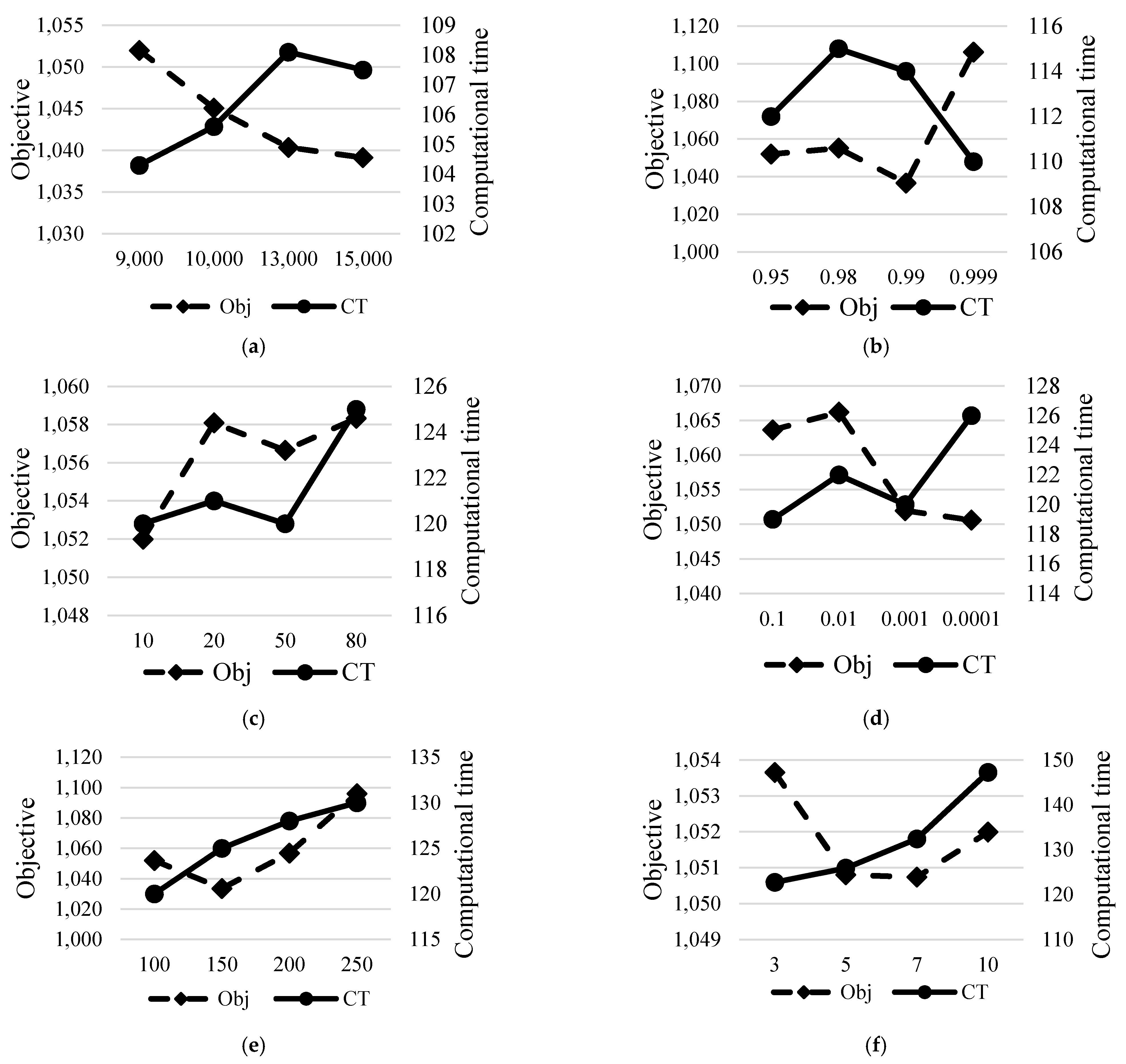
Six parameters are required for the 2^k factorial design: T₀, T_F, α, I_iter, N_{non-improving}, and M_restart. Each parameter consists of four levels as follows:

-

I_iter = 9000, 10,000, 13,000, 15,000;

-

α = 0.90, 0.95, 0.98, 0.99;

-

T₀ = 10, 20, 50, 80;

-

T_F = 0.1, 0.01, 0.001, 0.0001;

-

N_{non-improving} = 100, 150, 200, 250;

-

M_restart = 3, 5, 7, 10.

First, the one-factor-at-a-time (OFAT) approach is used to generate low and high levels for the 2^k factorial design prior to the actual parameter setting. Low and high levels are generated for each parameter from the OFAT approach to conduct the factorial design of the experiment, as depicted in

Table 2. Parameters for the 2^k factorial design of the experiment.

Parameter	Low (−)	High (+)
Iiter	13,000	15,000
α	0.95	0.99
T0	10	50
TF	0.001	0.0001
Nnon-improving	100	150
Mrestart	3	7

. Parameter values may influence the solution quality and computational time, and therefore this study conducts sensitivity analyses to observe the effects.

Figure 5 illustrates that I_iter and T_F tend to influence solution quality and computational time. As I_iter or T_F increases, the space for exploring solutions becomes larger, and so the chances of obtaining better solutions will increase. However, these efforts need more computational time. In contrast to I_iter and T_F, α does not affect solution quality or computational time, whereas T₀ does slightly affect the performance of the proposed algorithm. Increasing the value of this parameter does not always improve solution quality or reduce computational time.

When N_{non-improving} or M_restart increases, one needs significantly more time to solve the problem, but it is not always followed by an increase in the quality of the solution. Based on the design of the experiment and the sensitivity analyses, it seems that the setting I_iter = 15000, α = 0.99, T₀ = 10, T_F = 0.001, N_{non-improving} = 100, and M_restart = 7 provide the best results. Therefore, these parameter values are used to run the proposed SARS.

5.3. Computational Results

5.3.1. Verification of SARS for Solving the PCP Datasets

The first experiment’s results are presented in

Table 3. Comparison between SARS and HVNTS on small PCP instances.

Instance	n	C	S	T	m	HVNTS	SARS		Gap a
						Obj	Obj	CT
p1_s	15	50	0	Inf	5	658.39	658.39	48.913	0.00
p2_s	15	50	0	Inf	5	623.63	623.62	48.737	0.00
p3_s	15	50	0	Inf	5	632.40	632.41	49.146	0.00
p4_s	15	50	0	Inf	4	604.09	604.08	46.99	0.00
p5_s	15	50	0	Inf	7	781.59	781.59	54.513	0.00
p6_s	15	50	5	80	5	636.64	636.66	53.743	0.00
p7_s	15	50	5	80	5	617.44	617.41	49.59	−0.01
p8_s	15	50	5	80	5	628.40	628.40	49.672	0.00
p9_s	15	50	5	80	5	714.60	724.60	50.914	1.40
p10_s	15	50	5	96	5	632.40	632.41	50.742	0.00
Average						652.96	653.96	50.30	0.14

^a Gap = (obj of SARS − obj of HVNTS)/obj of HVNTS × 100%.

and

Table 4. Comparison between SARS and HVTNS on large PCP instances.

Instance	n	C	S	T	m	HVNTS		SARS		Gap a
						Obj	CT	Obj	CT
p1	50	160	0	Inf	5	865.88	6.74	865.88	70.46	0.00
p2	75	140	0	Inf	10	1434.56	16.01	1441.91	102.92	0.51
p3	100	200	0	Inf	8	1350.61	12.11	1352.66	125.93	0.15
p4	150	200	0	Inf	12	1803.87	63.96	1808.40	190.47	0.25
p5	199	200	0	Inf	17	2357.36	117.31	2365.06	251.70	0.33
p6	50	160	10	160	6	947.11	7.52	947.11	71.25	0.00
p7	75	140	10	128	11	1523.32	22.31	1527.01	104.23	0.24
p8	100	200	10	184	9	1443.38	35.10	1441.95	134.52	−0.10
p9	150	200	10	160	14	2078.35	42.08	1990.52	186.81	−4.23
p10	199	200	10	160	18	2532.90	220.38	2455.28	241.45	−3.06
p11	120	200	0	inf	7	1148.29	39.00	1127.59	145.63	−1.80
p12	100	200	0	inf	10	1284.99	19.87	1284.99	132.51	0.00
p13	120	200	50	576	11	1609.42	23.01	1518.84	165.59	−5.63
p14	100	200	90	832	11	1626.39	31.18	1520.88	137.56	−6.49
Average						1571.89	46.90	1546.29	147.22	−1.42

^a Gap = (obj of SARS − obj of HVNTS)/obj of HVNTS × 100%.

. The first column denotes the name of the instances. The subsequent five columns denote the feature of the instances described above. The following columns present the performance of HVTNS and the proposed SARS, respectively. Based on executing SARS in ten replications for each instance, the performance of the two algorithms is represented by both the best objective value (Obj) and the computational time (CT) of the best objective value. The last column describes the percentage gap between the best objective values of the two algorithms. Since there is no report of the computational time for small instances of PCP dataset in Yu et al. [14], the performance of HVTNS in Table 3 is only represented by the best objective value.

Table 3 shows that the proposed SARS can give a solution quality as good as HVNTS with an average gap of 0.14% in small PCP instances. Table 4 shows the computational results in large PCP instances. It implies that SARS implementation is unable to provide a better solution than HVNTS for instances p2, p3, p4, p5, and p7. However, for instances p8, p9, p10, p11, p13, and p14, the result obtained by SARS is superior compared to HVNTS in terms of objective value. Overall, the proposed SARS outperforms HVTNS in terms of average objective value of all large instance. Particularly, the average percentage gap of the objective value between SARS and HVNTS is −1.42%. Although the average computational time required by SARS is higher than that of HVTNS, it is still acceptable. The result indicates that the performance of SARS is as good as HVNTS, if not better, while the computational time is still reasonable.

5.3.2. Comparison of SARS with Other Algorithms on VRPTW Benchmark Instances

Table 5. Comparison of SARS with other optimal solution heuristics on the VRPTW dataset with 25 customers.

Instance	Optimal Solution			SARS			Gap
	TD	NV	CT	TD	NV	CT
C101	191.3	3	0.6	191.3	3	9.7	0.00
C102	190.3	3	1.9	190.3	3	9.6	0.00
C103	190.3	3	4.0	190.3	3	9.3	0.00
C104	186.9	3	8.5	186.9	3	9.5	0.00
C105	191.3	3	0.6	191.3	3	9.8	0.00
C106	191.3	3	0.6	191.3	3	9.5	0.00
C107	191.3	3	0.6	191.3	3	9.5	0.00
C108	191.3	3	0.6	191.3	3	9.4	0.00
C109	191.3	3	0.9	191.3	3	8.8	0.00
C201	214.7	2	a	214.7	2	4.0	0.00
C202	214.7	2	a	214.7	2	4.9	0.00
C203	214.7	2	a	214.7	2	2.9	0.00
C204	213.1	2	a	213.1	2	2.6	0.00
C205	214.7	2	a	214.7	2	3.0	0.00
C206	214.7	2	a	214.7	2	2.9	0.00
C207	214.5	2	a	214.5	2	3.0	0.00
C208	214.5	2	a	214.5	2	3.7	0.00
R101	617.1	8	0.2	617.1	8	5.0	0.00
R102	547.1	7	0.5	547.1	7	3.0	0.00
R103	454.6	5	0.9	454.6	5	4.4	0.00
R104	416.9	4	1.3	416.9	4	2.7	0.00
R105	530.5	6	0.3	530.5	6	4.8	0.00
R106	465.4	3	1.3	465.4	3	2.8	0.00
R107	424.3	4	1.5	424.3	4	3.1	0.00
R108	397.3	4	18.6	397.3	4	2.7	0.00
R109	441.3	5	0.4	441.3	5	2.7	0.00
R110	444.1	4	5.9	444.1	4	3.9	0.00
R111	428.8	5	2.0	428.8	5	3.9	0.00
R112	393.0	4	14.6	393	4	4.9	0.00
R201	463.3	4	1.9	463.3	4	2.9	0.00
R202	410.5	4	18.8	410.5	4	2.9	0.00
R203	391.4	3	355.4	391.4	3	5.1	0.00
R204	355.0	2	b	355	2	3.7	0.00
R205	393.0	3	21.4	393	3	2.8	0.00
R206	374.4	3	988.7	374.4	3	2.7	0.00
R207	361.6	3	9296.8	361.6	3	2.7	0.00
R208	328.2	1	b	328.2	1	2.8	0.00
R209	370.7	2	1991.4	370.7	2	5.3	0.00
R210	404.6	3	2417.7	404.6	3	6.7	0.00
R211	350.9	2	27,998.8	350.9	2	5.8	0.00
RC101	461.1	4	0.7	461.1	4	4.1	0.00
RC102	351.8	3	0.6	351.8	3	5.9	0.00
RC103	332.8	3	4.0	332.8	3	5.2	0.00
RC104	306.6	3	6.9	306.6	3	4.5	0.00
RC105	411.3	4	3.1	411.3	4	5.9	0.00
RC106	345.5	3	7.7	345.5	3	5.2	0.00
RC107	298.3	3	0.7	298.3	3	9.2	0.00
RC108	294.5	3	4.3	294.5	3	10.4	0.00
RC201	360.2	3	a	360.2	3	6.0	0.00
RC202	338.0	3	6386.7	338	3	3.1	0.00
RC203	326.9	3	b	326.9	3	3.2	0.00
RC204	299.7	3	b	299.7	3	9.4	0.00
RC205	338.0	3	57.9	338	3	3.8	0.00
RC206	324.0	3	82,387.5	324	3	3.8	0.00
RC207	298.3	3	220,991.2	298.3	3	7.3	0.00
RC208	269.1	2	b	269.1	2	6.6	0.00

^a = running time set to 2 until 25,000 s [53]. ^b = no mention of specific computing time [54]. Gap = (TD of SARS − TD of optimal solution)/TD of optimal solution × 100%.

,

Table 6. Comparison of SARS with other heuristics in the currently published papers on the VRPTW dataset with 100 customers (average best solution for each instance).

		C1	C2	R1	R2	RC1	RC2
BKS	TD	828.38	589.86	1180.36	888.67	1339.24	1014.5
	NV	10.0	3.0	13.1	5.1	12.8	6.1
CGH [28] a	TD	828.38	589.86	1183.38	899.90	1341.67	1015.90
	NV	10.0	3.0	13.3	5.5	12.9	6.5
	TD gap (%)	0.00	0.00	0.27	1.36	0.16	0.15
	Average CT	3600
	Average gap (%)	0.37
PITSH [29] b	TD	828.38	589.86	1209.19	951.17	1385.90	1120.53
	NV	10.0	3.0	12.0	2.7	11.5	3.3
	TD gap (%)	0.00	0.00	2.53	6.99	3.23	9.85
	Average CT	2357
	Average gap (%)	3.78
CPLA [31]a	TD	828.38	589.86	1232.13	922.48	1355.36	1106.00
	NV	10.0	3.0	11.9	3.1	12.0	3.4
	TD gap (%)	0.00	0.00	4.67	3.50	1.25	8.60
	Average CT	-
	Average gap (%)	3.1
HSFLA [32] a	TD	828.38	589.86	1210.34	951.03	1384.17	1119.24
	NV	10.0	3.0	11.2	2.7	11.5	3.3
	TD gap (%)	0.00	0.00	2.65	6.97	3.09	9.72
	Average CT	112
	Average gap (%)	3.77
tabu–ABC [34] a	TD	828.38	590.40	1187.90	891.24	1361.08	1017.47
	NV	10.0	3.0	13.5	4.7	13.3	5.5
	TD gap (%)	0.00	0.09	0.72	0.23	1.66	0.29
	Average CT	560
	Average gap (%)	0.49
SARS b	TD	828.38	589.86	1191.81	894.47	1367.64	1024.55
	NV	10.0	3.9	14.0	6.7	13.5	7.3
	TD gap (%)	0.00	0.00	1.01	0.57	2.08	0.90
	Average CT	117
	Average gap (%)	0.75

^a = population-based solution heuristic. ^b = single-based solution heuristic.

and

Table 7. Comparison of SARS with PITSH [29] and BKS on the VRPTW dataset with 100 customers (best solution for each instance).

Instance	BKS		PITSH [29]		SARS
	TD	NV	TD	NV	TD	NV	CT
C101	828.94	10	828.94	10	828.94	10	34.41
C102	828.94	10	828.94	10	828.94	10	64.70
C103	828.06	10	828.07	10	828.06	10	42.58
C104	824.77	10	824.78	10	824.77	10	39.95
C105	828.94	10	828.94	10	828.94	10	37.21
C106	828.94	10	828.94	10	828.94	10	38.00
C107	828.94	10	828.94	10	828.94	10	38.03
C108	828.94	10	828.94	10	828.94	10	40.56
C109	828.94	10	828.94	10	828.94	10	39.43
C201	591.55	3	591.56	3	591.55	3	33.58
C202	591.56	3	591.56	3	591.56	4	50.66
C203	591.17	3	591.17	3	591.17	4	133.34
C204	590.6	3	590.6	3	590.60	4	152.16
C205	588.88	3	588.88	3	588.88	4	102.72
C206	588.49	3	588.49	3	588.49	4	57.05
C207	588.29	3	588.29	3	588.29	3	119.90
C208	588.32	3	588.32	3	588.32	5	104.13
R101	1642.87	20	1650.8	19	1644.26	20	123.50
R102	1460.26	18	1486.12	17	1481.9	19	122.26
R103	1213.62	14	1294.23	13	1224.24	15	109.72
R104	981.2	10	981.2	10	1002.47	12	135.96
R105	1360.78	15	1377.11	14	1374.68	16	133.26
R106	1241.52	13	1252.62	12	1253.86	15	105.66
R107	1076.13	11	1104.66	10	1093.08	12	146.60
R108	948.57	10	963.99	9	954.48	11	115.38
R109	1151.84	13	1194.73	11	1159.72	13	188.29
R110	1080.36	11	1118.84	10	1081.78	12	116.81
R111	1053.5	12	1096.73	10	1061.29	12	117.78
R112	953.63	10	989.27	9	969.99	11	119.95
R201	1148.48	9	1252.37	4	1167.53	9	114.19
R202	1046.1	5	1191.7	3	1053.5	9	134.87
R203	884.02	5	941.08	3	891.61	7	171.39
R204	750.4	4	825.52	2	744.92	5	105.27
R205	960.75	5	994.43	3	978.74	8	146.25
R206	898.91	5	906.14	3	900.29	7	160.37
R207	809.72	4	890.61	2	809.36	5	134.03
R208	723.14	5	726.82	2	721.01	4	136.85
R209	863.12	5	909.16	3	875.47	6	160.38
R210	927.54	5	939.37	3	930.86	8	248.89
R211	763.22	4	885.71	2	765.87	6	138.37
RC101	1623.58	15	1696.95	14	1664.06	17	108.57
RC102	1466.84	14	1554.75	12	1489.22	15	110.98
RC103	1261.67	11	1261.67	11	1290.62	12	205.65
RC104	1135.48	10	1135.48	10	1140.64	10	160.80
RC105	1518.6	16	1633.72	13	1553.95	16	137.99
RC106	1377.35	13	1424.73	11	1417.87	14	132.24
RC107	1212.83	12	1232.2	11	1251.51	13	162.17
RC108	1117.53	11	1147.69	10	1133.25	11	130.32
RC201	1271.78	7	1406.94	4	1287.05	9	96.13
RC202	1113.53	8	1367.09	3	1109.51	9	109.19
RC203	941.81	5	1050.64	3	962.63	7	200.41
RC204	798.41	3	798.46	3	797.42	4	109.55
RC205	1161.81	7	1297.65	4	1186.54	9	130.72
RC206	1059.89	7	1153.61	3	1083.78	7	150.00
RC207	976.4	7	1061.14	3	984.38	8	153.98
RC208	792.33	5	828.71	3	785.07	5	152.26
Average	981.14	8.5	1021.41	7.3	990.23	9.4	117.24

The italic font indicates that the proposed SARS outperforms PITSH on the corresponding instance. The bold font implies that the proposed SARS obtains a new BKS.

summarize the results of the second experiment, which show the performance of SARS in solving both small and large VRPTW benchmark instances. In each table, column “TD” represents the total travel distance, “NV” denotes the number of vehicles, and “CT” indicates the computational time (s). Table 5 presents the results of the experiment of VRPTW with 25 customers. The SARS heuristic is compared with the optimal solution obtained by previous heuristics [52]. TD is the best result of 10 runs. On the basis of the experimental results, SARS obtains the optimal solution for all instances.

Table 6 presents the comparison of SARS to other heuristics from recently published papers on VRPTW. BKSs are summarized from Zhang et al. [34]. The table implies that in terms of solution quality, the results of SARS are equal to other algorithms and BKS on C1 and C2 instances and still comparable on other instances. Moreover, in terms of computational time, the proposed SARS outperforms CGH, PITSH, and tabu-ABC and is comparable with HSFLA. Note that Barbucha [31] did not report computational times. From the table, the other heuristics consist of two categories, namely single-based solution algorithms for PITSH by Cordeau and Maischberger [29] and population-based solution algorithms for CGH by Alvarenga et al. [28], CPLA by Barbucha [31], HSFLA by Luo et al. [32], and Tabu–ABC by Zhang et al. [34]. The table implies that the results of SARS are equal to other heuristics in terms of BKS on C1 and C2 instances and also still comparable in the other instances. In particular, SARS performs better in terms of the average gap with BKS when compared with another single-solution based algorithm from [29]. According to the table, the average gaps are 0.75% and 3.78% for SARS and PITSH [29], respectively.

Table 7 shows the comparison between SARS and PITSH [29] for each instance. The table shows that, in terms of solution quality, the proposed SARS outperforms PITSH for 34 of the 56 instances (italic font). Moreover, SARS generates six new BKSs (in bold font) in instances R204, R207, R208, RC202, RC204, and RC208. Furthermore, in terms of computational time, the proposed SARS also outperforms PITSH. Note that Cordeau and Maischberger [29] reported only average computational times of PITSH as presented in Table 6.

The third experiment compares the results of SARS and CPLEX. In addition, since SARS is modified from SA, this experiment also compares results of SARS and SA.

Table 8. Comparison among CPLEX, SA, and SARS on the PCPTW dataset with 25 customers.

Instance	CPLEX			SA			SARS			Gap1	Gap2
	NV	TD	CT	NV	TD	CT	NV	TD	CT
C101	3	368.92	0.31	3	368.92	1.6	3	368.92	44.0	0.00	0.00
C102	3	368.92	0.64	3	368.92	1	3	368.92	10.1	0.00	0.00
C103	3	365.31	18,000	3	365.31	1	3	365.31	9.8	0.00	0.00
C104	3	365.31	18,000	3	365.31	1.6	3	365.31	10.2	0.00	0.00
C105	3	368.92	0.34	3	368.92	2.5	3	368.92	10.4	0.00	0.00
C106	3	368.92	0.94	3	368.92	1.3	3	368.92	10.6	0.00	0.00
C107	3	368.92	1.37	3	368.92	1.1	3	368.92	10.6	0.00	0.00
C108	3	368.92	119.15	3	368.92	2	3	368.92	10.5	0.00	0.00
C109	3	367.50	5503.9	3	367.50	1.2	3	367.50	10.8	0.00	0.00
C201	2	353.14	0.61	2	353.14	1.3	2	353.14	9.7	0.00	0.00
C202	1	301.65	16.38	1	301.65	1.3	1	301.65	9.3	0.00	0.00
C203	1	301.15	174.59	1	301.15	1.6	1	301.15	8.9	0.00	0.00
C204	1	283.99	18,000	1	283.99	1.9	1	283.99	9.0	0.00	0.00
C205	2	353.14	0.45	2	353.14	1.8	2	353.14	9.5	0.00	0.00
C206	2	353.14	1.08	2	353.14	1.9	2	353.14	9.3	0.00	0.00
C207	1	347.98	72.2	1	347.98	1.5	1	347.98	8.9	0.00	0.00
C208	1	307.38	129.51	1	307.38	2.1	1	307.38	9.4	0.00	0.00
R101	8	1025.13	0.36	8	1025.1	1.2	8	1025.13	11.0	0.00	0.00
R102	7	912.14	461.09	7	912.14	1.7	7	912.14	10.3	0.00	0.00
R103	4	682.44	4536.54	4	682.44	15.5	4	682.44	41.3	0.00	0.00
R104	4	652.59	18,000	4	652.59	14.7	4	652.59	45.0	0.00	0.00
R105	5	815.75	1565.75	5	815.75	2	5	815.75	7.1	0.00	0.00
R106	4	769.45	3736.85	4	769.45	1.2	4	769.45	15.5	0.00	0.00
R107	4	654.27	14,010.3	4	654.27	14.3	4	654.27	41.5	0.00	0.00
R108	3	578.18	18,000	3	578.18	22.6	3	578.18	47.0	0.00	0.00
R109	4	673.54	6.93	4	673.54	15	4	673.54	43.3	0.00	0.00
R110	4	662.34	18,000	4	660.37	1.5	4	660.37	42.6	−0.30	−0.30
R111	4	652.33	18,000	4	652.33	2.1	4	652.33	7.7	0.00	0.00
R112	4	636.84	18,000	4	635.47	1.7	4	635.47	8.7	−0.22	−0.22
R201	2	614.01	5.08	2	614.01	0.9	2	614.01	5.7	0.00	0.00
R202	2	541.13	398.13	2	541.13	1.8	2	541.13	6.7	0.00	0.00
R203	2	505.41	18,000	2	505.35	1.6	2	505.35	8.7	−0.01	−0.01
R204	1	448.92	18,000	1	448.92	1	1	448.92	10.0	0.00	0.00
R205	2	516.48	274.89	2	516.48	13.9	2	516.48	42.3	0.00	0.00
R206	1	457.37	3007.72	1	457.37	14.3	1	457.37	33.2	0.00	0.00
R207	1	437.33	18,000	1	437.33	2.1	1	437.33	7.4	0.00	0.00
R208	1	384.78	18,000	1	384.78	2.4	1	384.78	5.9	0.00	0.00
R209	1	470.49	1049.65	1	470.49	1.4	1	470.49	7.4	0.00	0.00
R210	2	507.99	5321.04	2	507.99	1.3	2	507.99	13.1	0.00	0.00
R211	1	417.45	18,000	1	417.45	29.9	1	417.45	29.9	0.00	0.00
RC101	4	560.32	1.12	4	560.32	1.3	4	560.32	11.8	0.00	0.00
RC102	3	418.82	38.51	3	418.82	1.6	3	418.82	10.6	0.00	0.00
RC103	3	403.59	6683.77	3	403.59	1	3	403.59	11.1	0.00	0.00
RC104	3	383.39	18,000	3	383.39	1.4	3	383.39	9.4	0.00	0.00
RC105	4	516.61	715.43	4	516.61	1.8	4	516.61	9.3	0.00	0.00
RC106	3	406.66	7.1	3	406.66	1.8	3	406.66	8.8	0.00	0.00
RC107	3	386.53	18,000	3	386.53	1.9	3	386.53	12.9	0.00	0.00
RC108	3	382.39	18,000	3	382.39	2.3	3	382.39	12.6	0.00	0.00
RC201	2	477.54	1.53	2	477.54	2.5	2	477.54	12.0	0.00	0.00
RC202	3	406.92	307.53	3	406.92	12.3	3	406.92	37.1	0.00	0.00
RC203	2	397.47	18,000	2	397.47	1.6	2	397.47	11.3	0.00	0.00
RC204	1	347.98	18,000	1	347.98	1.6	1	347.98	14.5	0.00	0.00
RC205	3	408.82	6.01	3	408.82	1.6	3	408.82	13.3	0.00	0.00
RC206	2	393.43	55.05	2	393.43	1.9	2	393.43	13.3	0.00	0.00
RC207	2	358.21	8019.47	2	358.21	1.1	2	358.21	15.8	0.00	0.00
RC208	2	320.42	18,000	2	320.42	1.5	2	320.42	12.7	0.00	0.00
Average	2.7	473.19	7127.43	2.7	473.13	4.07	2.7	473.13	16.2	−0.01	−0.01

,

Table 9. Comparison among CPLEX, SA, and SARS on the PCPTW dataset with 50 customers.

Instance	CPLEX			SA			SARS			Gap1	Gap2
	NV	TD	CT	NV	TD	CT	NV	TD	CT
C101	5	641.76	0.1	5	641.76	20.3	5	641.76	59.8	0.00	0.00
C102	5	641.15	18,000	5	641.15	20.4	5	641.15	59.0	0.00	0.00
C103	5	638.15	18,000	5	638.15	20.5	5	638.15	64.4	0.00	0.00
C104	5	637.16	18,000	5	637.00	23.4	5	637.00	104.7	−0.03	−0.03
C105	5	641.37	1.1	5	641.37	20.3	5	641.37	58.3	0.00	0.00
C106	5	641.37	0.3	5	641.37	20.4	5	641.37	58.5	0.00	0.00
C107	5	641.37	0.4	5	641.37	20.1	5	641.37	58.5	0.00	0.00
C108	5	641.37	486.79	5	641.37	20.7	5	641.37	59.6	0.00	0.00
C109	5	640.77	18,000	5	640.77	20.6	5	640.77	58.9	0.00	0.00
C201	3	557.57	0.1	3	557.57	19.7	3	557.57	55.4	0.00	0.00
C202	2	532.59	18,000	2	532.59	19.1	2	532.59	59.9	0.00	0.00
C203	2	534.47	18,000	2	532.33	22.9	2	532.33	60.8	−0.40	−0.40
C204	2	475.16	18,000	2	500.34	23.1	2	499.17	103.0	5.30	5.05
C205	2	530.13	2.7	3	557.19	19.3	3	557.19	76.7	5.10	5.10
C206	2	529.57	18,000	3	557.19	20.7	3	557.19	76.7	5.22	5.22
C207	2	526.34	18,000	2	550.77	20.3	3	556.98	102.2	4.64	5.82
C208	2	504.56	18,000	2	504.56	24.4	2	504.56	73.3	0.00	0.00
R101	11	1634.31	0.5	12	1638.94	22.8	12	1638.94	75.3	0.28	0.28
R102	10	1423.39	18,000	10	1423.40	24	10	1423.4	92.4	0.00	0.00
R103	8	1226.01	18,000	8	1230.56	25.1	8	1223.73	90.8	0.37	−0.19
R104	6	988.75	18,000	6	989.55	22.7	6	988.75	76.4	0.08	0.00
R105	8	1366.16	30.0	9	1375.38	34.5	9	1375.38	86.1	0.67	0.67
R106	7	1191.89	18,000	8	1225.30	41.5	8	1224.34	110.3	2.80	2.72
R107	7	1111.03	18,000	7	1127.02	22.6	6	1065.79	115.7	1.44	−4.07
R108	6	988.86	18,000	6	977.91	50.4	6	977.91	155.8	−1.11	−1.11
R109	8	1228.97	18,000	8	1232.27	26	7	1187.81	97.6	0.27	−3.35
R110	8	1194.47	18,000	7	1122.37	30.9	7	1122.62	103.6	−6.04	−6.02
R111	7	1127.79	18,000	7	1108.90	41	7	1109.35	92.2	−1.67	−1.64
R112	7	1076.95	18,000	7	1068.80	42.1	7	1068.8	128.7	−0.76	−0.76
R201	3	1017.19	11.3	4	1053.60	25.1	4	1035.53	112.4	3.58	1.80
R202	3	908.92	18,000	4	931.10	21.2	3	909.71	85.5	2.44	0.09
R203	3	790.54	18,000	3	790.54	21	3	790.54	103.4	0.00	0.00
R204	2	658.69	18,000	2	642.62	27.4	2	641.97	108.5	−2.44	−2.54
R205	2	853.59	18,000	3	924.28	19.2	3	876.29	81.8	8.28	2.66
R206	3	848.88	18,000	2	793.24	19.1	2	788.30	77.3	−6.55	−7.14
R207	3	779.05	18,000	2	704.68	24	2	704.68	79.0	−9.55	−9.55
R208	2	637.89	18,000	2	637.93	29.1	2	636.2	85.5	0.01	−0.26
R209	2	772.45	18,000	3	798.81	23.2	3	776.25	94.8	3.41	0.49
R210	3	845.74	18,000	3	825.93	25.5	3	816.23	92.9	−2.34	−3.49
R211	3	779.77	18,000	3	744.04	33.9	2	688.53	88.8	−4.58	−11.7
RC101	8	1084.02	37.61	9	1119.86	22.9	8	1084.02	92.6	3.31	0.00
RC102	7	916.34	18,000	7	916.39	24.2	7	916.34	105.8	0.01	0.00
RC103	6	805.26	18,000	6	805.26	31.9	6	805.26	65.6	0.00	0.00
RC104	5	664.57	18,000	5	663.20	37.1	5	663.2	106.7	−0.21	−0.21
RC105	8	1044.16	18,000	8	1041.06	28.2	8	1041.06	89.3	−0.30	−0.30
RC106	6	820.24	18,000	6	820.24	20.8	6	820.24	86.5	0.00	0.00
RC107	6	770.92	18,000	6	770.92	20.9	6	770.92	69.4	0.00	0.00
RC108	6	745.42	18,000	6	744.37	39	6	744.37	97.7	−0.14	−0.14
RC201	5	754.00	2.1	5	754.00	20.2	5	754	60.1	0.00	0.00
RC202	4	708.04	18,000	5	712.51	23	5	713.51	93.3	0.63	0.77
RC203	4	651.65	18,000	4	653.65	32.1	4	653.65	96.0	0.31	0.31
RC204	3	528.02	18,000	2	523.42	36.7	2	520.29	93.5	−0.87	−1.46
RC205	4	727.39	18,000	5	732.96	20.7	5	732.96	57.4	0.77	0.77
RC206	4	705.16	18,000	5	716.49	20.8	4	705.16	72.6	1.61	0.00
RC207	4	662.88	18,000	4	654.51	33.6	4	654.51	82.5	−1.26	−1.26
RC208	3	578.67	18,000	3	568.70	35.1	3	560.41	98.2	−1.72	−3.16
Average	4.8	813.80	14,153.1	4.9	814.67	26.0	4.84	808.44	85.57	0.19	−0.48

and

Table 10. Comparison among CPLEX, SA, and SARS on the PCPTW dataset with 100 customers.

Instance	CPLEX			SA			SARS			Gap1	Gap2
	NV	TD	CT	NV	TD	CT	NV	TD	CT
C101	10	1306.01	7.3	10	1306.01	36.9	10	1306.01	135.5	0.00	0.00
C102	10	1306.01	18,000	10	1306.01	36.8	10	1306.01	110.7	0.00	0.00
C103	10	1306.01	18,000	10	1303.01	51.7	10	1303.01	125.9	−0.23	−0.23
C104	10	1316.3	18,000	10	1302.24	61.3	10	1302.24	177.2	−1.07	−1.07
C105	10	1305.62	4.6	10	1305.62	38.2	10	1305.62	131.6	0.00	0.00
C106	10	1305.62	17.0	10	1305.62	56.4	10	1305.62	97.4	0.00	0.00
C107	10	1305.62	32.7	10	1305.62	52.7	10	1305.62	146.5	0.00	0.00
C108	10	1305.24	18,000	10	1305.24	42.2	10	1305.24	169.9	0.00	0.00
C109	10	1555.74	18,000	10	1305.24	41.3	10	1305.24	141.0	−16.10	−16.10
C201	3	818.06	13.2	3	818.06	48.9	3	818.06	89.5	0.00	0.00
C202	3	818.06	3191.2	3	818.06	66.9	3	818.06	93.1	0.00	0.00
C203	3	824.39	18,000	3	817.67	47.0	3	817.67	161.3	−0.82	−0.82
C204	3	823.6	18,000	4	899.27	96.8	4	899.27	186.3	9.19	9.19
C205	3	815.38	689.8	3	815.38	46.6	4	904.61	199.0	0.00	10.94
C206	3	814.99	18,000	3	814.99	51.5	3	814.99	191.4	0.00	0.00
C207	3	814.79	18,000	3	814.79	34.1	3	814.79	143.9	0.00	0.00
C208	3	814.82	18,000	4	915.8	64.1	3	814.82	205.9	12.39	0.00
R101	19	2632.3	1.9	20	2700.79	74.8	19	2643.37	153.3	2.60	0.42
R102	17	2378.95	18,000	18	2433.95	110.2	17	2398.52	236.7	2.31	0.82
R103	15	2125.63	18,000	15	2100.26	128.7	14	2040.24	231.9	−1.19	−4.02
R104	11	1719.6	18,000	11	1678.83	108.8	10	1614.76	233.5	−2.37	−6.10
R105	14	2129.27	18,000	16	2265.29	52.1	15	2186.55	190.0	6.39	2.69
R106	14	2080.36	18,000	14	2064.23	72.3	14	2042.94	263.8	−0.78	−1.80
R107	12	1836.13	18,000	12	1835.86	90.6	12	1806.67	300.7	−0.01	−1.60
R108	11	1681.64	18,000	10	1583.57	103.7	10	1577.02	240.9	−5.83	−6.22
R109	13	2011.64	18,000	14	2010.34	64.2	14	2006.66	199.6	−0.06	−0.25
R110	14	2013.51	18,000	13	1880.81	73.1	13	1887.7	198.2	−6.59	−6.25
R111	13	1951.33	18,000	13	1877.2	129.7	12	1812.26	227.1	−3.80	−7.13
R112	13	1898.37	18,000	12	1734.86	79.1	11	1645.18	247.4	−8.61	−13.34
R201	5	1522.33	18,000	8	1652.15	61.4	7	1621.1	219.5	8.53	6.49
R202	6	1511.66	18,000	6	1434.72	119.5	6	1479.13	219.6	−5.09	−2.15
R203	5	1357.32	18,000	5	1280.39	52.1	5	1226.83	190.7	−5.67	−9.61
R204	4	1090.13	18,000	4	1050.44	59.5	4	1048.07	203.3	−3.64	−3.86
R205	5	1406.38	18,000	5	1330.02	67.7	5	1303.99	162.2	−5.43	−7.28
R206	4	1316.52	18,000	5	1255.04	114.7	5	1226.62	283.2	−4.67	−6.83
R207	5	1219.39	18,000	4	1097.45	94.1	4	1097.48	174.0	−10.00	−10.00
R208	4	1055.72	18,000	3	954.69	62.5	3	948.92	218.1	−9.57	−10.12
R209	5	1236.51	18,000	5	1239.73	53.7	5	1234.7	221.3	0.26	−0.15
R210	5	1454.27	18,000	6	1298.12	74.0	4	1183.89	196.7	−10.74	−18.59
R211	5	1325.75	18,000	4	1085.95	60.0	4	1069.47	184.9	−18.09	−19.33
RC101	15	2180.09	18,000	17	2310.51	53.9	16	2266.83	164.1	5.98	3.98
RC102	14	2036.69	18,000	14	2016.92	92.1	14	2040.72	194.4	−0.97	0.20
RC103	12	1835	18,000	12	1784.43	99.3	12	1800.83	219.7	−2.76	−1.86
RC104	11	1628.36	18,000	11	1622.13	99.1	11	1613.02	187.2	−0.38	−0.94
RC105	16	2214.91	18,000	16	2211.38	68.6	15	2154.06	227.1	−0.16	−2.75
RC106	13	1908.64	18,000	14	1969.25	82.9	14	1970.76	204.9	3.18	3.25
RC107	13	1897.3	18,000	12	1727.55	71.6	12	1726.75	189.4	−8.95	−8.99
RC108	13	1815.58	18,000	12	1682.22	85.0	11	1658.12	263.8	−7.35	−8.67
RC201	6	1562.17	18,000	9	1675.84	63.5	7	1612.73	185.4	7.28	3.24
RC202	6	1504.54	18,000	7	1507.28	60.6	7	1495.52	208.4	0.18	−0.60
RC203	5	1330.16	18,000	6	1316.05	102.6	5	1249.11	250.9	−1.06	−6.09
RC204	4	1385.52	18,000	5	1132.91	47.7	4	1083.5	205.3	−18.23	−21.80
RC205	7	1529.79	18,000	7	1528.79	45.4	7	1547.78	188.5	−0.07	1.18
RC206	5	1585.34	18,000	7	1469.66	77.0	7	1448.7	285.0	−7.30	−8.62
RC207	7	1425.75	18,000	7	1397.64	92.6	6	1327.52	145.4	−1.97	−6.89
RC208	6	1247.01	18,000	5	1180.22	91.3	5	1138.13	183.5	−5.36	−8.73
Average	8.7	1510.68	15,499.3	8.9	1479.22	71.7	8.6	1458.63	193.0	−2.08	−3.33

show the comparison of the PCPTW datasets with 25, 50, and 100 customers, respectively. Each table contains the results of the three methods. Each method consists of columns NV, TD, and CT representing the number of vehicles, objective value, and computational time (s), respectively. Columns Gap1 and Gap2 show the gap between CPLEX with SA and SARS, respectively. Gap1 is calculated by ((TD of SA − TD of CPLEX)/TD of CPLEX) × 100%, whereas Gap2 is calculated by ((TD of SARS − TD of CPLEX)/TD of CPLEX) × 100%.

In Table 8, CPLEX generated an optimal solution for 37 instances and ran for 5 h to generate the upper bound for 19 instances. Both SA and SARS could also achieve all optimal solutions provided by CPLEX in significantly shorter computational time. CPLEX could not solve the remaining instances to optimality, while our SARS yielded a better solution for three instances and the same solutions for 16 other instances. The average gap of SARS is −0.01%.

Table 9 shows that CPLEX achieved optimal solution for 12 instances and ran for 5 h to generate the upper bound for 44 instances. The proposed SARS achieved an optimal solution for eight instances and produced equal or better results compared with those of the upper bounds for 33 instances. The average gap is −0.48%. Table 10 shows that CPLEX also achieved an optimal solution for 8 instances, and ran for 5 h to generate upper bounds for the remaining 48 instances. The proposed SARS obtained optimal solutions for 6 instances, and the average gap is −3.33%.

The three tables report that the proposed SARS is advantageous in improving SA. The proposed SARS does not appear superior to solve PCPTW with 25 customers. As the size of the problem increases, the algorithm shows its superiority compared with SA heuristic. This phenomenon is shown in Table 8 for PCPTW with 25 customers, where averages of Gap1 and Gap2 are equal at −0.01%. The values are different in Table 9 and Table 10 for PCPTW with 50 customers and 100 customers, respectively. In these two tables, average Gap2 is larger than average Gap1, implying that SARS is better than SA in terms of solution quality. In terms of computational time, SARS needs more time to implement the restart strategy. The higher computational time of SARS is still acceptable since the results of SARS are better than those obtained by SA.

Table 11. Summary of the instances that obtain the optimal solution between CPLEX and SARS.

Instance Size	CPLEX			SARS			Gap *
	N-Optimal	Total TD	Total CT	N-Optimal	Total TD	Total CT
Small	37	17,889.71	56,231.32	37	17,889.71	593.5	0.00
Medium	12	10,150.62	573	9	10,209.87	853.3	0.58
Large	8	10,306.67	3957.7	6	10,406.97	1045.9	0.97
Total	57	38,347.00	60,762.02	52	38,506.55	2492.7	0.42

* Gap = (Total TD of SARS − Total TD of CPLEX)/Total TD of CPLEX × 100%.

compares the performances of CPLEX and the proposed SARS in finding optimal solutions. The values of the table are summarized from the results presented in Table 8, Table 9 and Table 10. The percentage gap in the last column shows that for small size instances, both methods result in the same number of instances, yielding the optimal solution. The last row of the Gap column presents the percentage gap between SARS and CPLEX in terms of solution quality. It shows that the proposed SARS has a gap of less than 1% compared to that of CPLEX, yet SARS still has faster computational time than CPLEX.

5.3.3. Analysis of the Restart Strategy

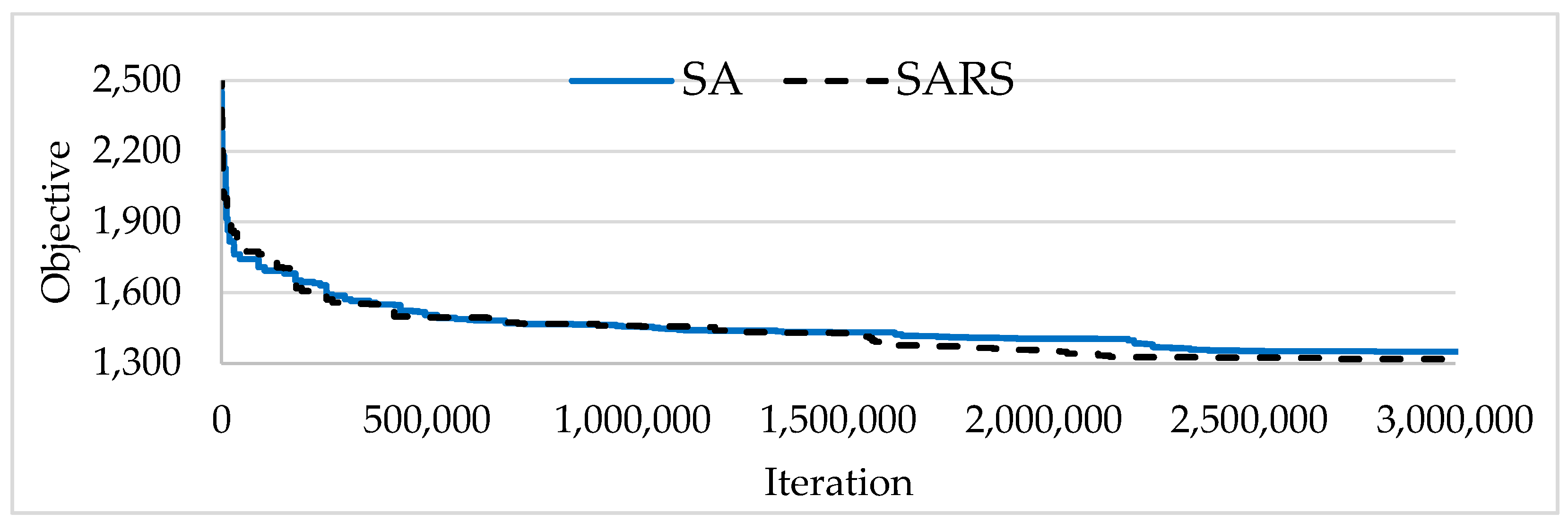
This subsection analyzes the restart strategy. Figure 6 shows the convergence history of SA and SARS, which appears in blue and black lines, respectively. Both methods are executed with one run on instance RC207 of the PCPTW dataset. Based on the figure, both methods are able to converge during the searching process. However, SARS is able to give a better solution compared to SA.

6. Conclusions and Future Research

The scientific novelty of this study is the development of a mathematical programming model and an effective SARS algorithm for solving PCPTW, which can be implemented to extend PCP by considering customer time windows in small- and medium-sized enterprises that hire freelance workers to reduce operational cost. The mathematical model of PCPTW is developed and solved by using CPLEX. SARS, which is an extended SA that utilizes a restart strategy, is proposed to tackle PCPTW.

To investigate the effectiveness of the proposed algorithm, we test it on PCP and well-known VRPTW datasets. The experimental results show that SARS is comparable with HVTNS in solving PCP instances and with several algorithms on VRPTW datasets. Moreover, on VRPTW datasets, SARS outperforms another single-solution based algorithm in terms of the average gap with BKS, and generates new BKSs for six large instances.

In solving the PCPTW dataset, the experimental results show that SARS outperforms CPLEX in terms of the solution quality and the computational time for all sizes of the problem scale. Furthermore, utilizing the restart strategy enables SARS to outperform SA in terms of solution quality. Although employing the restart strategy needs more computational time, the results indicate that the longer computational time of SARS is still reasonable.

The developed formulation and solution techniques can be extended to a practical strategy for companies in order to reduce operational cost by hiring freelance workers. However, current studies are limited to considering cost minimization. In practice, the proposed model might not yet cover several realistic situations that could arise.

Future research can consider other realistic situations and use a more practical dataset. Factors beyond cost optimization such as customer satisfaction and workers’ preferences are becoming a social topic that cannot be ignored and should be addressed. Moreover, the involvement of a heterogeneous fleet, split delivery, and multiple time windows can also extend the problem. Optimization methods such as particle swarm optimization, genetic algorithm, and other advanced algorithms can be used further to increase solution quality.

References

- Niu, Y.; Yang, Z.; Chen, P.; Xiao, J. Optimizing the green open vehicle routing problem with time windows by minimizing comprehensive routing cost. J. Clean. Prod. 2018, 171, 962–971. [Google Scholar] [CrossRef]
- Shen, L.; Tao, F.; Wang, S. Multi-depot open vehicle routing problem with time windows based on carbon trading. Int. J. Environ. Res. Public Health 2018, 15, 2025. [Google Scholar] [CrossRef]
- Solomon, M.M. Algorithms for the vehicle routing and scheduling problems with time window constraints. Oper. Res. 1987, 35, 254–265. [Google Scholar] [CrossRef]
- Ticha, H.B.; Absi, N.; Feillet, D.; Quilliot, A. Multigraph modeling and adaptive large neighborhood search for the vehicle routing problem with time windows. Comput. Oper. Res. 2019, 104, 113–126. [Google Scholar] [CrossRef]
- Bernardo, M.; Du, B.; Pannek, J. A simulation-based solution approach for the robust capacitated vehicle routing problem with uncertain demands. Transp. Lett. 2020, 1–10. [Google Scholar] [CrossRef]
- Bertazzi, L.; Secomandi, N. Faster rollout search for the vehicle routing problem with stochastic demands and restocking. Eur. J. Oper. Res. 2018, 270, 487–497. [Google Scholar] [CrossRef]
- Marković, D.; Petrovć, G.; Ćojbašić, Ž.; Stanković, A. The vehicle routing problem with stochastic demands in an urban area–A case study. Facta Univ. Ser. Mech. Eng. 2020, 18, 107–120. [Google Scholar] [CrossRef]
- Huang, Y.; Zhao, L.; Woensel, T.V.; Gross, J.-P. Time-dependent vehicle routing problem with path flexibility. Transp. Res. Part B Methodol. 2017, 95, 169–195. [Google Scholar] [CrossRef]
- Norouzi, N.; Sadegh-Amalnick, M.; Tavakkoli-Moghaddam, R. Modified particle swarm optimization in a time-dependent vehicle routing problem: Minimizing fuel consumption. Optim. Lett. 2017, 11, 121–134. [Google Scholar] [CrossRef]
- Rincon-Garcia, N.; Waterson, B.; Cherrett, T.J.; Salazar-Arrieta, F. A metaheuristic for the time-dependent vehicle routing problem considering driving hours regulations–An application in city logistics. Transp. Res. Part A Policy Pract. 2018, 137, 429–446. [Google Scholar] [CrossRef]
- Chen, P.; Golden, B.; Wang, X.; Wasil, E. A novel approach to solve the split delivery vehicle routing problem. Int. Trans. Oper. Res. 2017, 24, 27–41. [Google Scholar] [CrossRef]
- Gschwind, T.; Bianchessi, N.; Irnich, S. Stabilized branch-price-and-cut for the commodity-constrained split delivery vehicle routing problem. Eur. J. Oper. Res. 2019, 278, 91–104. [Google Scholar] [CrossRef]
- Xia, Y.; Fu, Z.; Pan, L.; Duan, F. Tabu search algorithm for the distance-constrained vehicle routing problem with split deliveries by order. PLoS ONE 2018, 13, e0195457. [Google Scholar] [CrossRef]
- Yu, V.F.; Redi, A.A.N.P.; Halim, C.; Jewpanya, P. The path cover problem: Formulation and a hybrid metaheuristic. Expert Syst. Appl. 2020, 146, 113107. [Google Scholar] [CrossRef]
- Salari, M.; Toth, P.; Tramontani, A. An ILP improvement procedure for the open vehicle routing problem. Comput. Oper. Res. 2010, 37, 2106–2120. [Google Scholar] [CrossRef][Green Version]
- Repoussis, P.P.; Tarantilis, C.D.; Ioannou, G. The open vehicle routing problem with time windows. J. Oper. Res. Soc. 2007, 58, 355–367. [Google Scholar] [CrossRef]
- Yu, B.; Yang, Z.; Yao, B. A hybrid algorithm for vehicle routing problem with time windows. Expert Syst. Appl. 2011, 38, 435–441. [Google Scholar] [CrossRef]
- Sariklis, D.; Powell, S. A Heuristic Method for the Open Vehicle Routing Problem. J. Oper. Res. Soc. 2000, 51, 564–573. [Google Scholar] [CrossRef]
- Clarke, G.; Wright, J.W. Scheduling of vehicles from a central depot to a number of delivery points. Oper. Res. 1964, 12, 568–581. [Google Scholar] [CrossRef]
- Foster, B.A.; Ryan, D.M. An integer programming approach to the vehicle scheduling problem. J. Oper. Res. Soc. 1976, 27, 367–384. [Google Scholar] [CrossRef]
- Gillet, B.E.; Miller, L.E.; Johnson, J.G. Vehicle dispatching—Sweep algorithm and extensions. In Disaggregation; Springer: Dordrecht, The Netherlands, 1979; pp. 471–483. [Google Scholar]
- Toth, P.; Vigo, D. The Vehicle Routing Problem; SIAM Monographs on Discrete Mathematics and Applications; Society for Industrial and Applied Mathematics: Philadelphia, PA, USA, 2002. [Google Scholar]
- Cordeau, J.-F.; Laporte, G. Tabu search heuristics for the vehicle routing problem. Metaheuristic Optim. Mem. Evol. 2005, 30, 145–163. [Google Scholar]
- Xia, Y.; Fu, Z. An adaptive tabu search algorithm for the open vehicle routing problem with split deliveries by order. Wirel. Pers. Commun. 2018, 103, 595–609. [Google Scholar] [CrossRef]
- Xia, Y.; Fu, Z. Improved tabu search algorithm for the open vehicle routing problem with soft time windows and satisfaction rate. Clust. Comput. 2019, 22, 8725–8733. [Google Scholar] [CrossRef]
- Lalla-Ruiz, E.; Mes, M. Mathematical formulations and improvements for the multi-depot open vehicle routing problem. Optim. Lett. 2020, 15, 271–286. [Google Scholar] [CrossRef]
- Tan, K.C.; Chew, Y.H.; Lee, L. A hybrid multiobjective evolutionary algorithm for solving vehicle routing problem with time windows. Comput. Optim. Appl. 2006, 34, 115–151. [Google Scholar] [CrossRef]
- Alvarenga, G.B.; Mateus, G.R.; de Tomi, G. A genetic and set partitioning two-phase approach for the vehicle routing problem with time windows. Comput. Oper. Res. 2007, 34, 1561–1584. [Google Scholar] [CrossRef]
- Cordeau, J.-F.; Maischberger, M. A parallel iterated tabu search heuristic for vehicle routing problems. Comput. Oper. Res. 2012, 39, 2033–2050. [Google Scholar] [CrossRef]
- Gong, Y.-J.; Zhang, J.; Liu, O.; Huang, R.-Z.; Chung, H.S.-H.; Shi, Y.-H. Optimizing the vehicle routing problem with time windows: A discrete particle swarm optimization approach. IEEE Trans. Syst. Man Cybern. Part C (Appl. Rev.) 2012, 42, 254–267. [Google Scholar] [CrossRef]
- Barbucha, D. A cooperative population learning algorithm for vehicle routing problem with time windows. Neurocomputing 2014, 146, 210–229. [Google Scholar] [CrossRef]
- Luo, J.; Li, X.; Chen, M.-R.; Liu, H. A novel hybrid shuffled frog leaping algorithm for vehicle routing problem with time windows. Inf. Sci. 2015, 316, 266–292. [Google Scholar] [CrossRef]
- Yassen, E.T.; Ayob, M.; Nazri, M.Z.A.; Sabar, N.R. Meta-harmony search algorithm for the vehicle routing problem with time windows. Inf. Sci. 2015, 325, 140–158. [Google Scholar] [CrossRef]
- Zhang, D.; Cai, S.; Ye, F.; Si, Y.-W.; Nguyen, T.T. A hybrid algorithm for a vehicle routing problem with realistic constraints. Inf. Sci. 2017, 394, 167–182. [Google Scholar] [CrossRef]
- Yang, X.-S. Nature-Inspired Optimization Algorithms; Elsevier: Amsterdam, The Netherlands, 2014. [Google Scholar]
- Keskin, M.; Çatay, B. A matheuristic method for the electric vehicle routing problem with time windows and fast chargers. Comput. Oper. Res. 2018, 100, 172–188. [Google Scholar] [CrossRef]
- Goel, R.; Maini, R.; Bansal, S. Vehicle routing problem with time windows having stochastic customers demands and stochastic service times: Modelling and solution. J. Comput. Sci. 2019, 34, 1–10. [Google Scholar] [CrossRef]
- Song, M.-X.; Li, J.-Q.; Han, Y.-Q.; Han, Y.-Y.; Liu, L.-L.; Sun, Q. Metaheuristics for solving the vehicle routing problem with the time windows and energy consumption in cold chain logistics. Appl. Soft Comput. 2020, 95, 106561. [Google Scholar] [CrossRef]
- Metropolis, N.; Rosenbluth, A.W.; Rosenbluth, M.N.; Teller, A.H.; Teller, E. Equation of state calculations by fast computing machines. J. Chem. Phys. 1953, 21, 1087–1092. [Google Scholar] [CrossRef]
- Kirkpatrick, S.; Gelatt, J.C.; Vecchi, M.P. Optimization by simmulated annealing. Science 1983, 220, 671–680. [Google Scholar] [CrossRef]
- Eglese, R. Simulated annealing: A tool for operational research. Eur. J. Oper. Res. 1990, 46, 271–281. [Google Scholar] [CrossRef]
- Marandi, F.; Ghomi, S.F. Network configuration multi-factory scheduling with batch delivery: A learning-oriented simulated annealing approach. Comput. Ind. Eng. 2019, 132, 293–310. [Google Scholar] [CrossRef]
- Rabbouch, B.; Saâdaoui, F.; Mraihi, R. Empirical-type simulated annealing for solving the capacitated vehicle routing problem. J. Exp. Theor. Artif. Intell. 2020, 32, 437–452. [Google Scholar] [CrossRef]
- Wei, L.; Zhang, Z.; Zhang, D.; Leung, S.C. A simulated annealing algorithm for the capacitated vehicle routing problem with two-dimensional loading constraints. Eur. J. Oper. Res. 2018, 265, 843–859. [Google Scholar] [CrossRef]
- Yu, V.F.; Redi, A.A.N.P.; Hidayat, Y.A.; Wibowo, O.J. A simulated annealing heuristic for the hybrid vehicle routing problem. Appl. Soft Comput. 2017, 53, 119–132. [Google Scholar] [CrossRef]
- Yu, V.F.; Winarno; Lin, S.-W.; Gunawan, A. Design of a two-echelon freight distribution system in an urban area considering third-party logistics and loading–unloading zones. Appl. Soft Comput. 2020, 97(Part B), 106707. [Google Scholar] [CrossRef]
- Marti, R. Multi-start methods. In Handbook of Metaheuristics; Glover, F., Konchenberger, G.A., Eds.; Kluwer Academic Publishers: Dordrecht, The Netherlands, 2003; pp. 355–368. [Google Scholar]
- Lin, S.-W.; Yu, V.F. A simulated annealing heuristic for the multiconstraint team orienteering problem with multiple time windows. Appl. Soft Comput. 2015, 37, 632–642. [Google Scholar] [CrossRef]
- Yu, V.F.; Lin, S.-W.; Lee, W.; Ting, C.-J. A simulated annealing heuristic for the capacitated location routing problem. Comput. Ind. Eng. 2010, 58, 288–299. [Google Scholar] [CrossRef]
- Yu, V.F.; Lin, S.-Y. A simulated annealing heuristic for the open location-routing problem. Comput. Oper. Res. 2015, 62, 184–196. [Google Scholar] [CrossRef]
- Coy, S.P.; Golden, B.L.; Runger, G.C.; Wasil, E.A. Using Experimental Design to Find Effective Parameter Setting for Heuristic. J. Heuristics 2000, 7, 77–97. [Google Scholar] [CrossRef]
- VRPTW Best Known Solutions. Available online: http://web.cba.neu.edu/~msolomon/heuristi.htm (accessed on 15 July 2020).
- Cook, W.; Rich, J.L. A Parallel Cutting-Plane Algorithm for the Vehicle Routing Problem with Time Windows; In Technical Report TR99-04; Computational and Applied Mathematics, Rice University: Housten, TX, USA, 1999. [Google Scholar]
- Chabrier, A. Vehicle routing problem with elementary shortest path based column generation. Comput. Oper. Res. 2006, 33, 2972–2990. [Google Scholar] [CrossRef]