Application of Induced Preorderings in Score Function-Based Method for Solving Decision-Making with Interval-Valued Fuzzy Soft Information

Abstract

Ranking interval-valued fuzzy soft sets is an increasingly important research issue in decision making, and provides support for decision makers in order to select the optimal alternative under an uncertain environment. Currently, there are three interval-valued fuzzy soft set-based decision-making algorithms in the literature. However, these algorithms are not able to overcome the issue of comparable alternatives and, in fact, might be ignored due to the lack of a comprehensive priority approach. In order to provide a partial solution to this problem, we present a group decision-making solution which is based on a preference relationship of interval-valued fuzzy soft information. Further, corresponding to each parameter, two crisp topological spaces, namely, lower topology and upper topology, are introduced based on the interval-valued fuzzy soft topology. Then, using the preorder relation on a topological space, a score function-based ranking system is also defined to design an adjustable multi-steps algorithm. Finally, some illustrative examples are given to compare the effectiveness of the present approach with some existing methods.

1. Introduction

Dealing with vagueness and uncertainty, rather than exactness, in most real-world situations is the main problem in data-analysis sciences and decision-making. Many mathematical theories and tools such as probability theory, fuzzy set theory [1], interval-valued fuzzy set theory [2], intuitionist fuzzy set theory [3], rough set theory [4] and soft set theory [5] have been implemented to handle this problem, with the latter allowing researchers to deal with parametric data. Nowadays, soft sets theory contributes to a vast range of applications, particularly in decision-making. In this regard, many important results have been achieved, from parameter reduction to new ranking models.

Many soft set extensions and their applications have been discussed in previous studies, such as fuzzy soft sets [6,7,8,9,10,11,12,13] intuitionistic fuzzy sets [14,15,16,17], rough soft sets [18,19] and fuzzy soft topology [20,21,22,23]. The interval-valued fuzzy soft method was first used for decision-making problems by Son [24]. He applied this method by using the comparison table. Yang et al. [25] developed the method presented in [7] for an interval-valued fuzzy soft set and then, applied the concept of interval-valued fuzzy choice values to propose an approach for solving decision-making problems. The notion of level set in decision-making based on interval-valued fuzzy soft sets was introduced by Feng et al. [26] and then, the level soft set for interval-valued fuzzy soft sets was developed, further see [27]. Khameneh et al. [28,29,30] introduced the preference relationship for both fuzzy soft sets and intuitionistic fuzzy soft sets and then selected an optimal option for group decision-making problems by defining a new function value. In addition, interval-valued fuzzy soft sets have also been applied to various fields, for example information measure [31,32,33,34], decision making [35,36,37,38], matrix theory [39,40,41], and parameter reduction [37,38,42].

Recently, Ma et al. [43] introduced an average and an antitheses table for interval-valued fuzzy soft sets and then selected an optimal option for group decision-making problems through the score value. Ma et al. [44] developed two methods [26,45] to solve decision-making problems by providing a new efficient decision-making algorithm and also considering added objects. However, these methods did not address the problem of incomparable alternatives because they lack a comprehensive priority approach. In order to solve these issues, this paper proposes an application of the induced preorderings based method for solving decision-making with interval-valued fuzzy soft information.Our contributions are as follows:

1

Proposing application of induced preordering based method for solving decision-making with interval-valued fuzzy soft information.

2

Proposing a novel score function of interval-valued fuzzy soft sets that selects an optimal option for group decision-making problems.

3

A real-life example is given to compare the effectiveness of this approach with some existing methods.

2. Preliminaries

In this section, we recall some definitions and properties of interval-valued fuzzy sets ($IVF$) and interval-valued fuzzy soft sets $\left(IVFS\right)$. Note that, throughout this paper, X and E denote the sets of objects and parameters, respectively. ${\mathbb{I}}^X$ and ${\left[\mathbb{I}\right]}^X,$ where $\mathbb{I}=[0,1]$ and $\left[\mathbb{I}\right]=\left\{\right[a,b],a\le b,a,b\in \mathbb{I}\}$ denote, respectively, the set of all fuzzy subsets and the set of all interval-valued fuzzy subsets of X.

Definition 1.

Ref. [2] A pair $(f,X)$, is called an $IVF$ subset of X if f is a mapping given by $f:X\to \left[\mathbb{I}\right]$ such that for any $x\in X,f\left(x\right)=[f^{-}\left(x\right),f^{+}\left(x\right)]$ is a closed subinterval of $[0,1]$ where $f^{-}\left(x\right)$ and $f^{+}\left(x\right)$ are referred to as the lower and upper degrees of membership x to f and $0\le f^{-}\left(x\right)\le f^{+}\left(x\right)\le 1$.

In 1999, Molodtsov [5] defined the concept of soft sets (SS) for the first time as a pair of $(f,E)$ or $f_E$ such that E is a parameter set and f is the mapping $f:E\to 2^X$ where for any $e\in E,f\left(e\right)$ is a subset of X. By combining the concepts of soft sets and interval-valued fuzzy sets, a new hybrid tool was defined as the following.

Definition 2.

Ref. [25] A pair $(f,E)$ is called an $IVFS$ set over X if the mapping f is given by $f:E\to {\left[\mathbb{I}\right]}^X$ where for any $e\in E$ and $x\in X$, $f\left(e\right)\left(x\right)=[f^{-}\left(e\right)\left(x\right),f^{+}\left(e\right)\left(x\right)]$.

Consider two $IVFSs$ $f_E,g_E$ over the common universe X. The union of $f_E$ and $g_E$, denoted by $f_E\tilde{\vee }{g}_E$, is the $IVFSs$ ${\left(f\tilde{\vee }g\right)}_E$, where $\forall e\in E$ and any $x\in X$, we have $\left(f\tilde{\vee }g\right)\left(e\right)\left(x\right)=[max\{f_e^{-}\left(x\right),g_e^{-}\left(x\right)\},max\{f_e^{+}\left(x\right),g_e^{+}\left(x\right)\}]$. The intersection of $f_E$ and $g_E$, denoted by $f_E\tilde{\wedge }{g}_E$, is the $IVFSs$ ${\left(f\tilde{\wedge }g\right)}_E$, where $\forall e\in E$ and $\forall x\in X$, we have $\left(f\tilde{\wedge }g\right)\left(e\right)\left(x\right)=[min\{f_e^{-}\left(x\right),g_e^{-}\left(x\right)\},min\{f_e^{+}\left(x\right),g_e^{+}\left(x\right)\}]$. The complement of $f_E$ is denoted by $f_E^c$ and is defined by $f^c:E\to {\left[\mathbb{I}\right]}^X$ where $\forall e\in E$ and any $x\in X$, $f^c\left(e\right)\left(x\right)=[1-f_e^{+}\left(x\right),1-f_e^{-}\left(x\right)]$. The null $IVFSs$, denoted by ${\varnothing }_E$, is defined as an $IVFSs$ over X such that $f_e^{-}\left(x\right)=f_e^{+}\left(x\right)=0$ for all $e\in E$ and any $x\in X$. The absolute $IVFSs$, denoted by $X_E$, is defined as an $IVFSs$ over X where $f_e^{-}\left(x\right)=f_e^{+}\left(x\right)=1,\forall e\in E$ and any $x\in X$.

Using the matrix form of interval-valued fuzzy relations, authors in [39] represented a finite IVFSs $f_E$ as the following $n\times m$ matrix

$$f_E={\left[[f_{ij}^{-},f_{ij}^{+}]\right]}_{n\times m}={\left[\begin{array}{ccc}[f_{e_1}^{-}\left(x_1\right),f_{e_1}^{+}\left(x_1\right)]& \dots & [f_{e_1}^{-}\left(x_m\right),f_{e_1}^{+}\left(x_m\right)]\\ ⋮& \dots & ⋮\\ [f_{e_{\mathrm{n}}}^{-}\left(x_1\right),f_{e_1}^{+}\left(x_1\right)]& \dots & [f_{e_n}^{-}\left(x_m\right),f_{e_1}^{+}\left(x_m\right)]\end{array}\right]}_{n\times m}$$

where $\mid E\mid =n$, $\mid X\mid =m$ and $f_{ij}^{-}=f_{e_i}^{-}\left(x_j\right)$, $f_{ij}^{+}=f_{e_i}^{+}\left(x_j\right)$ for $i=1,\dots ,n$ and $j=1,\dots ,m.$

Accordingly, the concepts of union, intersection, complement, etc., can be represented in a matrix format in the finite case.

Definition 3.

Ref. [46] A triplet $(X,E,\tau )$ is called an interval-valued fuzzy soft topological space (IVFST) if τ is a collection of interval-valued fuzzy soft subsets of X containing absolute and null $IVFSs$ and closed under arbitrary union and finite intersection.

Preorders and Topologies

In this subsection, we present some basic properties about the connection between preorders and topologies proposed by [47].

Topological structures and classical order structures are well recognised to have close relationships, which can be summarised as follows:

(1)

A subset A of X is called an upper set of X if $A=\uparrow A$, where $\uparrow A$ defined by $\uparrow A=\{y\in X:\exists x\in A,x\le y\},$ and X is a preordered set, and B is called a lower set $B=\downarrow B=\{y\in X:\exists x\in X,y\le x\}$.

(2)

The family of all upper subsets of x is a topology for a preorder set $(X,\le )$, which is called the Alexandrov topology induced in $(X,\le )$.

(3)

A topological space $(X,\tau )$ is defined by $x\le y$ if and only if $x\in U$, then $y\in U$ for each open set U of $X,$ or equivalently $x\in c\left\{y\right\},$ where $c\left\{y\right\},$ is the closure of $\left\{y\right\}.$ Then, ≤ is a preorder on $X,$ called the specialization order $(X,\tau )$ on X.

3. Construction Tow Preorderings in Lower and Upper Spaces

By using the notion of $[{\alpha }_1,{\alpha }_2]$-level sets of interval-valued fuzzy soft open sets in $(X,E,\tau )$, this section, introduces two topological spaces, known as lower and upper spaces, by which two preordering relations over the universal set X are investigated.

Definition 4.

Let $f_E$ be an IVFS set over X. Corresponding to each parameter $e\in E,$, we define two crisp sets, called α-upper-e crisp set and β-lower-e crisp set, where $\alpha =[{\alpha }_1,{\alpha }_2]\subset \mathbb{I},\beta =[{\beta }_1,{\beta }_2]\subset \mathbb{I}$ as the following:

$$\begin{array}{ccc}\hfill U.C.S_{\alpha }^f\left(e\right)& =& \{x\in X:[f_e^{-}\left(x\right),f_e^{+}\left(x\right)]>\alpha ,\alpha \subseteq [0,1)\}\hfill \\ & =& \{x\in X:f_e^{-}\left(x\right)>{\alpha }_1,f_e^{+}\left(x\right)>{\alpha }_2,{\alpha }_1,{\alpha }_2\in [0,1)\}\hfill \\ \hfill L.C.S_{\beta }^f\left(e\right)& =& \{x\in X:[f_e^{-}\left(x\right),f_e^{+}\left(x\right)]<\beta ,\beta \subseteq (0,1]\}\hfill \\ & =& \{x\in X:f_e^{-}\left(x\right)<{\beta }_1,f_e^{+}\left(x\right)<{\beta }_2,{\beta }_1,{\beta }_2\in (0,1]\}\hfill \end{array}$$

Proposition 1.

Let X be the set of objects, E be the set of parameters and $f_E$, $g_E$ be two $IVFSs$ over X. Suppose that the threshold intervals ${\alpha }_1,{\alpha }_2,\subseteq [0,1),$ and ${\beta }_1,{\beta }_2,\subseteq (0,1]$ are given such that ${\alpha }_1=[{\alpha }_1^{\star },{\alpha }_1^{\star \star }],{\alpha }_2=[{\alpha }_2^{\star },{\alpha }_2^{\star \star }],{\beta }_1=[{\beta }_1^{\star },{\beta }_1^{\star \star }]$ and ${\beta }_2=[{\beta }_2^{\star },{\beta }_2^{\star \star }]$. Consider the parameter $e\in E$.

1. 

If ${\alpha }_1\ge {\alpha }_2,$ then $U.C.S_{{\alpha }_1}^f\left(e\right)\subseteq U.C.S_{{\alpha }_2}^f\left(e\right).$ If ${\beta }_1\ge {\beta }_2,$ then $L.C.S_{{\beta }_2}^f\left(e\right)\subseteq L.C.S_{{\beta }_1}^f\left(e\right).$

2. 

If $f_E\tilde{\le }{g}_E,$ then $U.C{S}_{{\alpha }_1}^f\left(e\right)\subseteq U.C.S_{{\alpha }_1}^g\left(e\right)$ and $L.C.S_{{\beta }_1}^f\left(e\right)\subseteq L.C.S_{{\beta }_1}^g\left(e\right).$

3. 

If $f_E=X_E$, then $U.C.S_{{\alpha }_1}^f\left(e\right)=X$ and $L.C.S_{{\beta }_1}^f\left(e\right)=\varnothing .$ Moreover, if $f_E={\varnothing }_E$ then, $U.C{S}_{{\alpha }_1}^f\left(e\right)=\varnothing$ and $L.C{S}_{{\beta }_1}^f\left(e\right)=X.$

4. 

$U.C.S_{{\alpha }_1}^f(\neg e)=L.C{S}_{[1-{\alpha }_1^{\star \star },1-{\alpha }_1^{\star }]}^f\left(e\right)$ and $L.C{S}_{{\alpha }_1}^f(\neg e)=U.C{S}_{[1-{\alpha }_1^{\star \star },1-{\alpha }_1^{\star }]}^f\left(e\right).$

5. 

$U.C{S}_{{\alpha }_1}^{\neg f}\left(e\right)=L.C{S}_{[1-{\alpha }_1^{\star \star },1-{\alpha }_1^{\star }]}^f\left(e\right)$ and $L.C{S}_{{\alpha }_1}^{\neg f}(\neg e)=U.De{s}_{[1-{\alpha }_1^{\star \star },1-{\alpha }_1^{\star }]}^f\left(e\right).$

Proof. 

It is straightforward.    □

Theorem 1.

Let $(X,E,\tau )$ be an $IVFSTS.$ Suppose that the threshold intervals ${\alpha }_1,{\alpha }_2,\subseteq [0,1),$ and ${\beta }_1,{\beta }_2,\subseteq (0,1]$ are given such that $\alpha =[{\alpha }_1,{\alpha }_2]$ and $\beta =[{\beta }_1,{\beta }_2]$, then

1. 

The collection $\{U.C.S_{\alpha }^f\left(e\right):f_E\in \tau ,e\in E,\alpha \subseteq [0,1)\},$ denoted by ${\tau }_{e,\alpha }^u,$ is a topology over $X.$

2. 

The collection ${\mathfrak{B}}_{\beta }^l\left(e\right)=\{L.C.S_{\beta }^f\left(e\right):f_E\in \tau ,e\in E,\beta \subseteq (0,1]\},$ is a base for a topology over $X,$ denoted by ${\tau }_{e,\beta }^l.$

Proof. 

• (a)

  By Proposition 1, $X,\varnothing \in {\tau }_{e,\alpha }^u,$ since $X_E,{\varnothing }_E\in \tau .$

  (b)

  Let ${\{U.C.S_{\alpha }^{f_i}\left(e\right)\}}_{i\in I}$ be a subfamily of ${\tau }_{e,\alpha }^u.$ Then, we have ${\bigcup }_{i}U.C.S_{\alpha }^{f_i}\left(e\right)$$=U.C.S_{\alpha }^{\left({\tilde{\vee }}_{i\in I}{f}_i\right)}\left(e\right)\in {\tau }_{e,\alpha }^u,$ since ${\tilde{\vee }}_{i\in I}{f}_{iE}\in \tau$.

  (c)

  Let $U.C.S_{\alpha }^f\left(e\right)$ and $U.C.S_{\alpha }^g\left(e\right)$ be two open sets in ${\tau }_{e,\alpha }^u.$ Then, we have $U.C{S}_{\alpha }^f\left(e\right)\cap U.C.S_{\alpha }^g\left(e\right)=U.C.S_{\alpha }^{\left(f\tilde{\wedge }g\right)}\left(e\right)\in {\tau }_{e,\alpha }^u,$ since $f_E\tilde{\wedge }{g}_E\in \tau$. This completes the proof.

• (a)

  That $X\in {\mathfrak{B}}_{\beta }^l\left(e\right)$ is implied from ${\varnothing }_E$ is in $\tau$.

  (b)

  Let $L.C.S_{\beta }^f\left(e\right)$ and $L.C.S_{\beta }^g\left(e\right)$ in ${\mathfrak{B}}_{\beta }^l\left(e\right).$ Then, we have $L.C.S_{\beta }^f\left(e\right)\cap L.C.S_{\beta }^g\left(e\right)=L.C.S_{\beta }^{f\tilde{\vee }g}\left(e\right)\in {\mathfrak{B}}_{\beta }^l\left(e\right)$ that is implied form $f\tilde{\vee }g\in \tau .$

   □

Theorem 2.

Let $(X,E,\tau )$ be an $IVFSTS.$ Suppose that the threshold intervals ${\alpha }_1,{\alpha }_2,\subseteq [0,1),$ and ${\beta }_1,{\beta }_2,\subseteq (0,1]$ are given such that $\alpha =[{\alpha }_1,{\alpha }_2]$ and $\beta =[{\beta }_1,{\beta }_2].$

1. 

The binary relation ${\succsim }_{e,\alpha }^{\tau }$ on X defined by

$$y{⪰}_{e,\alpha }^{\tau }x\iff [\forall V\in {\tau }_{e,\alpha }^u:x\in V\Rightarrow y\in V]$$

is a preorder relation called α-upper-e preorder relation on $X.$

2. 

The binary relation ${⪯}_e^{\tau ,\beta }$ on X defined by

$$y{⪯}_e^{\tau ,\beta }x\iff [\forall U\in {\tau }_{e,\beta }^l:x\in U\Rightarrow y\in U]$$

is a preorder relation called β-lower-e preorder relation on $X.$

Proof. 

• For all $x\in X,$ obviously, $x{\succsim }_{e,\alpha }^{u}x,$ that is, “${\succsim }_{e,\alpha }^u$” is reflexive. Now, for all $x,y,z\in X,$ if $y{\succsim }_{e,\alpha }^{u}x,$ and $z{\succsim }_{e,\alpha }^{u}y,$ then, if for all $V\in {\tau }_{e,\alpha }^u$-open set, $x\in V,$ then $y\in V$ and $z\in V,$ so, $z{\succsim }_{e,\alpha }^{u}x,$ that is, “${\succsim }_{e,\alpha }^u$” is transitive. Thererfore, $(X,{\succsim }_{e,\alpha }^u)$ is a preordered set.
• A similar technique is used to prove the second part.

   □

Theorem 3.

Let $(X,E,\tau )$ be an $IVFSTS.$ Suppose that the threshold intervals ${\alpha }_1,{\alpha }_2,\subseteq [0,1),$ and ${\beta }_1,{\beta }_2,\subseteq (0,1]$ are given such that $\alpha =[{\alpha }_1,{\alpha }_2]$ and $\beta =[{\beta }_1,{\beta }_2].$

1. 

The binary relation ${\backsimeq }_{e,\alpha }^{\tau },$ defined by

$$y{\backsimeq }_{e,\alpha }^{\tau }x\iff [y{\succsim }_{e,\alpha }^{\tau }x,x{\succsim }_{e,\alpha }^{\tau }y]$$

is an equivalence relation over $X.$ If $y{\backsimeq }_{e,\alpha }^{\tau }x,$ then we say x and y are α-upper equivalent with to respect to the parameter $e.$

The equivalence relation ${\backsimeq }_{e,\alpha }^{\tau },$ generates the partition $P_{e,\alpha }^{\tau }$ of X where the equivalence classes are defined as ${\left[x\right]}_{e,\alpha }^{\tau }=\{z\in X:z{\backsimeq }_{e,\alpha }^{\tau }x$ and are called α-upper-e equivalence classes.

2. 

The binary relation ${\backsimeq }_e^{\tau ,\beta },$ where $\beta =[{\beta }_1,{\beta }_2],$

$$y{\backsimeq }_e^{\tau ,\beta }x\iff [y{\precsim }_e^{\tau ,\beta }x,x{\precsim }_e^{\tau ,\beta }y]$$

is an equivalence relation over $X.$ If $y{\backsimeq }_{e,\beta }^{\tau }x,$ then we say x and y are $[{\beta }_1,{\beta }_2]$-lower equivalent with to respect to the parameter $e.$ The equivalence relation ${\backsimeq }_e^{\tau ,\beta },$ generates the partition $P_e^{\tau ,\beta }$ of X where the equivalence classes are defined as ${\left[x\right]}_e^{\tau ,\beta }=\{z\in X:z{\backsimeq }_e^{\tau ,\beta }x$ and are called β-lower-e equivalence classes.

Proof. 

It is straightforward.    □

Preorder and Equivalence Matrices

Now, let the finite sets $X=\{x_1,\cdots ,x_m\}$ and $E=\{e_1,\cdots ,e_n\}$ be given as the sets of objects and parameters. Then, the previous properties can be represented by using the matrix form of $IVFS$ sets as the following.

Take an $IVFS$ set $f_E$ over X. First, for any $1\le i\le m$ and $1\le t\le n$, the concepts of $\alpha$-upper-$e_t$ and $\beta$-lower-$e_t$ matrices of $f_E$, where $\alpha ,\beta \subseteq \mathbb{I}$, can be formulated as the following two matrices (or row vectors)

$$U.C.S_{\alpha }{e}_t^f={\left[u_i^f(e_t,\alpha )\right]}_{1\times m}=\left\{\begin{array}{cc}1& \mathrm{if}{f}_{e_t}^{-}\left(x_i\right)>{\alpha }_1,f_{e_t}^{+}\left(x_i\right)>{\alpha }_2\\ 0& \mathrm{if}{f}_{e_t}^{-}\left(x_i\right)\le {\alpha }_1,f_{e_t}^{+}\left(x_i\right)\le {\alpha }_2\end{array}\right.$$

(1)

and

$$L.C.S_{\beta }{e}_t^f={\left[l_i^f(e_t,\beta )\right]}_{1\times m}=\left\{\begin{array}{cc}0& \mathrm{if}{f}_{e_t}^{-}\left(x_i\right)\ge {\beta }_1,f_{e_t}^{+}\left(x_i\right)\ge {\beta }_2\\ 1& \mathrm{if}{f}_{e_t}^{-}\left(x_i\right)<{\beta }_1,f_{e_t}^{+}\left(x_i\right)<{\beta }_2\end{array}\right.$$

(2)

where $\alpha =[{\alpha }_1,{\alpha }_1]$ and $\beta =[{\beta }_1,{\beta }_2]$ are the given threshold vectors.

Then, obviously, for any $e_t\in E$, the topologies ${\tau }_{e_t,\alpha }^u$ and ${\tau }_{e_t,\beta }^l$ can be represented by the collections

$${\tau }_{e_t,\alpha }^u=\{{\left[u_i^f(e_t,\alpha )\right]}_{1\times m}:\alpha \subseteq [0,1),f_E\in \tau ,1\le i\le m\}$$

and

$${\tau }_{e_t,\beta }^l=\{{\left[l_i^f(e_t,\beta )\right]}_{1\times m}:\beta \subseteq (0,1],f_E\in \tau ,1\le i\le m\}$$

where $\tau$ is the $IVFST$ on X.

Accordingly, the preorderings ${⪰}_{e_t,\alpha }^{\tau }$ and ${⪯}_{e_t}^{\tau ,\beta }$ can be represented by

$$x_i{⪰}_{e_t,\alpha }^{\tau }{x}_j\iff [\forall f_E\in \tau :u_j^f(e_t,\alpha )=1\Rightarrow u_i^f(e_t,\alpha )=1]$$

and

$$x_i{⪯}_{e_t}^{\tau ,\beta }{x}_j\iff [\forall f_E\in \tau :l_j^f(e_t,\beta )=1\Rightarrow l_i^f(e_t,\beta )=1]$$

where $x_i,x_j\in X$.

The matrix forms of the preorderings ${\succsim }_{e_t,\alpha }^{\tau }$ and ${\precsim }_{e_t}^{\tau ,\beta }$ are used to define two comparison matrices $G_{\alpha }\left(e_t\right)={\left[g_{\alpha }{\left(e_t\right)}_{ij}\right]}_{m\times m}$ and $S_{\beta }\left(e_t\right)={\left[s_{\beta }{\left(e_t\right)}_{ij}\right]}_{m\times m}$, which are two square matrices whose rows and columns are labeled by the objects of X, as below.

Definition 5.

Consider the binary relations ${\succsim }_{e_t,\alpha }^{\tau }$ and ${\precsim }_{e_t}^{\tau ,\beta }$ and threshold intervals $\alpha =[{\alpha }_1,{\alpha }_2],\beta =[{\beta }_1,{\beta }_2\subseteq \mathbb{I}$. Then, we define

$$G_{\alpha }\left(e_t\right)={\left[g_{\alpha }{\left(e_t\right)}_{ij}\right]}_{m\times m}:g_{[{\alpha }_1,{\alpha }_2]}{\left(e_t\right)}_{ij}=\left\{\begin{array}{cc}1& if{x}_i{\succsim }_{e_t,\alpha }^{\tau }{x}_j\\ 0& otherwis\end{array}\right.$$

(3)

and

$$S_{\beta }\left(e_t\right)={\left[s_{\beta }{\left(e_t\right)}_{ij}\right]}_{m\times m}:s_{[{\beta }_1,{\beta }_2]}{\left(e_t\right)}_{ij}=\left\{\begin{array}{cc}1& if{x}_i{\precsim }_{e_t}^{\tau ,\beta }{x}_j\\ 0& otherwis\end{array}\right.$$

(4)

Proposition 2.

Let $(X,E,\tau )$ be an $IVFST$ and $G_{\alpha }\left(e\right)$ and $S_{\beta }\left(e\right)$ be two matrices defined in Equations (3) and (4). Then,

1. 

For $1\le i\le m,g_{\alpha }{\left(e_t\right)}_{ii}=1$ and $s_{\beta }{\left(e_t\right)}_{ii}=1,$

2. 

If $g_{\alpha }{\left(e_t\right)}_{ij}=g_{\alpha }{\left(e_t\right)}_{jk}=1,$ then $g_{\alpha }{\left(e_t\right)}_{ik}=1.$ If $s_{\beta }{\left(e_t\right)}_{ij}=s_{\beta }{\left(e_t\right)}_{jk}=1,$ then $s_{\beta }{\left(e_t\right)}_{ik}=1.$

3. 

$G_{\alpha }\left(e_t\right)$ and $S_{\beta }\left(e_t\right)$ are symmetric matrices.

where $i,j,k\in \{1,\dots ,m\}$

Proof. 

It is straightforward.    □

Proposition 3.

Let $(X,E,\tau )$ be an $IVFSTS$ and $\alpha ,\beta \subseteq \mathbb{I},$ where $\alpha =[{\alpha }_1,{\alpha }_1]$ and $\beta =[{\beta }_1,{\beta }_2]$ are the threshold intervals, then

1. 

$G_{\alpha }\left(e_t\right)$ is an identity matrix if and only if $\neg \left(x_i{⪰}_{e_t\alpha }^{\tau }{x}_j\right),\forall i,j=1,\dots ,m$ and $i\ne j.$

2. 

$S_{\beta }\left(e_t\right)$ is an identity matrix if and only if $\neg \left(x_i{⪯}_{e_t}^{\tau ,\beta }{x}_j\right),\forall i,j=1,\dots ,m$ and $i\ne j.$

3. 

$G_{\alpha }\left(e_t\right)$ is a unit matrix if and only if $x_i{⪰}_{e_t,\alpha }^{\tau }{x}_j,\forall i,j=1,\dots ,m$ and $i\ne j$.

4. 

$S_{\beta }\left(e_t\right)$ is a unit matrix if and only if $x_i{⪯}_{e_t}^{\tau ,\beta }{x}_j,\forall i,j=1,\dots ,m$ and $i\ne j.$

Proof. 

It is straightforward.    □

Proposition 4.

Let $(X,E,\tau )$ be an $IVFSTS$ and $\alpha ,\beta \subseteq \mathbb{I},$ where $\alpha =[{\alpha }_1,{\alpha }_1],\beta =[{\beta }_1,{\beta }_2]$ are the threshold intervals, then

1. 

$G_{\alpha }\left(e_t\right)=I_m^U$ if and only if we have $x_1{⪰}_{e_t,\alpha }^{\tau }\cdots {⪰}_{e_t,\alpha }^{\tau }{x}_m$.

2. 

$S_{\beta }\left(e_t\right)=I_m^U$ if and only if $x_1{⪯}_{e_t}^{\tau ,\beta }\cdots {⪯}_{e_t}^{\tau ,\beta }{x}_m$.

3. 

$G_{\alpha }\left(e_t\right)=I_m^L$ if and only if $x_m{⪰}_{e_t,\alpha }^{\tau }\cdots {⪰}_{e_t,\alpha }^{\tau }{x}_1$.

4. 

$S_{\beta }\left(e_t\right)=I_m^L$ if and only if $x_m{⪯}_{e_t}^{\tau ,\beta }\cdots {⪯}_{e_t}^{\tau ,\beta }{x}_1$.

where $I_m^U,I_m^L$ are the upper and lower triangular matrix, respectively.

Proof. 

It is straightforward.    □

Analogously, the equivalence relations ${\backsimeq }_{e_t,\alpha }^{\tau }$ and ${\backsimeq }_{e_t}^{\tau ,\beta }$ can be applied to compute the following two square matrices

$E_{\alpha }^U\left(e_t\right)={\left[e_{\alpha }^u{\left(e_t\right)}_{ij}\right]}_{m\times m}$ and $E_{\beta }^L\left(e_t\right)={\left[e_{\beta }^l{\left(e_t\right)}_{ij}\right]}_{m\times m},$ respectively, where $\alpha =[{\alpha }_1,{\alpha }_2],\beta =[{\beta }_1,{\beta }_2]\subseteq \mathbb{I}$.

Definition 6.

Consider the binary relations ${\backsimeq }_{e_t,\alpha }^{\tau }$ and ${\backsimeq }_{e_t}^{\tau ,\beta }$ and threshold intervals $\alpha =[{\alpha }_1,{\alpha }_2],\beta =[{\beta }_1,{\beta }_2\subseteq \mathbb{I}$. We define

$$E_{\alpha }^U\left(e_t\right)={\left[e_{\alpha }^u{\left(e_t\right)}_{ij}\right]}_{m\times m}:e_{\alpha }^u{\left(e_t\right)}_{ij}=\left\{\begin{array}{cc}1& if{x}_i{\backsimeq }_{e_t,\alpha }^{\tau }{x}_j\\ 0& otherwis\end{array}\right.$$

(5)

and

$$E_{\beta }^L\left(e_t\right)={\left[e_{\beta }^l{\left(e_t\right)}_{ij}\right]}_{m\times m}:e_{\beta }^l{\left(e_t\right)}_{ij}=\left\{\begin{array}{cc}1& if{x}_i{\backsimeq }_{e_t}^{\tau ,\beta }{x}_j\\ 0& otherwis\end{array}\right.$$

(6)

Proposition 5.

Let $(X,E,\tau )$ be an $IVFST$ and $E_{\alpha }^U\left(e_t\right)$ and $E_{\beta }^L\left(e_t\right)$ be the comparison matrices defined in Equations (5) and (6). Then,

1. 

For any $1\le i\le m$: $e_{\alpha }^u{\left(e_t\right)}_{ii}=1$ and $e_{\beta }^l{\left(e_t\right)}_{ii}=1.$

2. 

$E^U\left(e_t\right)$ and $E^L\left(e_t\right)$ are symmetric matrices.

3. 

If $e_{\alpha }^u{\left(e_t\right)}_{ik}=e_{\alpha }^u{\left(e_t\right)}_{jk}=1,$ then $e_{\alpha }^u{\left(e_t\right)}_{ij}=e_{\alpha }^u{\left(e_t\right)}_{ji}=1$. If $e_{\beta }^l{\left(e_t\right)}_{ik}=e_{\beta }^l{\left(e_t\right)}_{jk}=1,$ then $e_{\beta }^l{\left(e_t\right)}_{ij}=e_{\beta }^l{\left(e_t\right)}_{ji}=1.$

4. 

If $e_{\alpha }^u{\left(e_t\right)}_{ki}=e_{\alpha }^u{\left(e_t\right)}_{kj}=1,$ then $e_{\alpha }^u{\left(e_t\right)}_{ij}=e_{\alpha }^u{\left(e_t\right)}_{ji}=1$. If $e_{\beta }^l{\left(e_t\right)}_{ki}=e_{\beta }^l{\left(e_t\right)}_{kj}=1,$ then $e_{\beta }^l{\left(e_t\right)}_{ij}=e_{\beta }^l{\left(e_t\right)}_{ji}=1.$

where $i,j,k\in \{1,\cdots ,m\}$

Proof. 

It is straightforward.    □

4. An Application in Decision-Making Problems

The main task in decision making methods is to rank the given candidates to find the optimum choice. Since the proposed preorderings, given in Section 3, are not total or linear, we define a score function S based on the entries of defined comparison matrices to obtain a new ranking system of objects according to preorderings ${\succsim }_{e_t,\alpha }^{\tau }$ and ${\precsim }_{e_t}^{\tau ,\beta }$.

Definition 7.

Let X and E be the universal sets of objects and parameters, respectively, and $\alpha ,\beta \subseteq \mathbb{I},$ where $\alpha =[{\alpha }_1,{\alpha }_1]$ and $\beta =[{\beta }_1,{\beta }_2]$, are the threshold intervals. The mapping $S=X\to \mathbb{R}$ defined by

$$\begin{array}{c}\hfill S\left(x_i\right)=S_i=\sum _{t=1}^n\left(\left[\sum _{j=1}^m{g}_{\alpha }{\left(e_t\right)}_{ij}-\sum _{j=1}^m{e}_{\alpha }^u{\left(e_t\right)}_{ij}\right]-\left[\sum _{j=1}^m{s}_{\beta }{\left(e_t\right)}_{ij}-\sum _{j=1}^m{e}_{\beta }^l{\left(e_t\right)}_{ij}\right]\right)\end{array}$$

where $x_i\in X$ and $S_i$ is score value of object $x_i$.

Example 1.

Suppose that $X=\{o_1,o_2,o_3,o_5\}$ be a set of 5 hotels in Langkawi and $E=\{e_1,\dots ,e_4\}$ be a set of parameters where for any $t=1,\dots ,4$ the parameter $e_t$ stands for “location”, “cleanliness”, “facilities”, and “ food”, respectively. Reviewers are classified into three groups: couples, solo travelers, and a group of friends. We consider these groups of reviewers as three different decision-makers, $f_1,f_2,f_3$, characterized based on the criteria $e_t\in E$. These three groups provide the following three $IVFS$ matrices $f_{1E},f_{2E},f_{3E}.$

• Step 1. The following three interval-valued fuzzy soft set $f_{sE}(s=1,2,3)$ that are given in Table 1, Table 2 and Table 3.

Table 1. $f_{1E}$.

${\mathit{f}}_{1\mathit{E}}$	${\mathit{o}}_1$	${\mathit{o}}_2$	${\mathit{o}}_3$	${\mathit{o}}_4$	${\mathit{o}}_5$
$e_1$	$[0.1,0.4]$	$[0.4,0.4]$	$[0.4,0.5]$	$[0,0.5]$	$[0.0,0.0]$
$e_2$	$[0.5,0.6]$	$[0.3,0.6]$	$[0.3,1.0]$	$[0.7,1.0]$	$[0.0,0.7]$
$e_3$	$[0.0,0.5]$	$[0.5,0.8]$	$[0.1,0.8]$	$[0.1,0.9]$	$[0.3,0.9]$
$e_4$	$[0.0,0.8]$	$[0.7,0.8]$	$[0.1,0.7]$	$[0.1,1.0]$	$[0.6,1.0]$

Table 1. $f_{1E}$.

${\mathit{f}}_{1\mathit{E}}$	${\mathit{o}}_1$	${\mathit{o}}_2$	${\mathit{o}}_3$	${\mathit{o}}_4$	${\mathit{o}}_5$
$e_1$	$[0.1,0.4]$	$[0.4,0.4]$	$[0.4,0.5]$	$[0,0.5]$	$[0.0,0.0]$
$e_2$	$[0.5,0.6]$	$[0.3,0.6]$	$[0.3,1.0]$	$[0.7,1.0]$	$[0.0,0.7]$
$e_3$	$[0.0,0.5]$	$[0.5,0.8]$	$[0.1,0.8]$	$[0.1,0.9]$	$[0.3,0.9]$
$e_4$	$[0.0,0.8]$	$[0.7,0.8]$	$[0.1,0.7]$	$[0.1,1.0]$	$[0.6,1.0]$

Table 2. $f_{2E}$.

${\mathit{f}}_{2\mathit{E}}$	${\mathit{o}}_1$	${\mathit{o}}_2$	${\mathit{o}}_3$	${\mathit{o}}_4$	${\mathit{o}}_5$
$e_1$	$[0.2,0.6]$	$[0.2,0.6]$	$[0.6,0.6]$	$[0.5,0.6]$	$[0.5,0.6]$
$e_2$	$[0.4,0.8]$	$[0.0,0.8]$	$[0.0,0.6]$	$[0.6,0.9]$	$[0.6,0.9]$
$e_3$	$[0.1,0.5]$	$[0.1,0.8]$	$[0.6,0.8]$	$[0.5,0.6]$	$[0.5,0.9]$
$e_4$	$[0.3,0.6]$	$[0.3,0.3]$	$[0.2,0.3]$	$[0.2,0.7]$	$[0.7,0.7]$

Table 2. $f_{2E}$.

${\mathit{f}}_{2\mathit{E}}$	${\mathit{o}}_1$	${\mathit{o}}_2$	${\mathit{o}}_3$	${\mathit{o}}_4$	${\mathit{o}}_5$
$e_1$	$[0.2,0.6]$	$[0.2,0.6]$	$[0.6,0.6]$	$[0.5,0.6]$	$[0.5,0.6]$
$e_2$	$[0.4,0.8]$	$[0.0,0.8]$	$[0.0,0.6]$	$[0.6,0.9]$	$[0.6,0.9]$
$e_3$	$[0.1,0.5]$	$[0.1,0.8]$	$[0.6,0.8]$	$[0.5,0.6]$	$[0.5,0.9]$
$e_4$	$[0.3,0.6]$	$[0.3,0.3]$	$[0.2,0.3]$	$[0.2,0.7]$	$[0.7,0.7]$

Table 3. $f_{3E}$.

${\mathit{f}}_{3\mathit{E}}$	${\mathit{o}}_1$	${\mathit{o}}_2$	${\mathit{o}}_3$	${\mathit{o}}_4$	${\mathit{o}}_5$
$e_1$	$[0.5,0.6]$	$[0.6,0.5]$	$[0.1,0.8]$	$[0.1,0.5]$	$[0.5,0.6]$
$e_2$	$[0.2,0.8]$	$[0.2,0.2]$	$[0.2,0.2]$	$[0.2,0.6]$	$[0.1,0.6]$
$e_3$	$[0.1,0.3]$	$[0.1,0.2]$	$[0.2,0.3]$	$[0.2,0.3]$	$[0.2,0.8]$
$e_4$	$[0.7,0.8]$	$[0.0,0.8]$	$[0.0,0.1]$	$[0.1,1.0]$	$[0.1,0.3]$

Table 3. $f_{3E}$.

${\mathit{f}}_{3\mathit{E}}$	${\mathit{o}}_1$	${\mathit{o}}_2$	${\mathit{o}}_3$	${\mathit{o}}_4$	${\mathit{o}}_5$
$e_1$	$[0.5,0.6]$	$[0.6,0.5]$	$[0.1,0.8]$	$[0.1,0.5]$	$[0.5,0.6]$
$e_2$	$[0.2,0.8]$	$[0.2,0.2]$	$[0.2,0.2]$	$[0.2,0.6]$	$[0.1,0.6]$
$e_3$	$[0.1,0.3]$	$[0.1,0.2]$	$[0.2,0.3]$	$[0.2,0.3]$	$[0.2,0.8]$
$e_4$	$[0.7,0.8]$	$[0.0,0.8]$	$[0.0,0.1]$	$[0.1,1.0]$	$[0.1,0.3]$

• Step 2. Assume that $[{\alpha }_1,{\alpha }_2]=[0.3,0.6]$ and $[\beta ,{\beta }_2=[0.2,0.4].$
• Step 3. The upper crisp matrices and lower crisp matrices, as below:

  $$f_1=\left[\begin{array}{cccccc}0& 0& 0& 0& 0& \\ 0& 0& 0& 1& 0& \\ 0& 1& 0& 0& 0& \\ 0& 1& 0& 0& 1& \end{array}\right],f_2=\left[\begin{array}{cccccc}0& 0& 0& 0& 0& \\ 1& 0& 0& 1& 1& \\ 0& 0& 1& 0& 1& \\ 0& 0& 0& 0& 1& \end{array}\right],f_3=\left[\begin{array}{cccccc}0& 1& 0& 0& 0& \\ 0& 0& 0& 0& 0& \\ 0& 0& 0& 0& 0& \\ 1& 0& 0& 0& 0& \end{array}\right]$$

  $$f_1=\left[\begin{array}{cccccc}0& 0& 0& 0& 1& \\ 0& 0& 0& 0& 0& \\ 0& 0& 0& 0& 0& \\ 0& 0& 0& 0& 0& \end{array}\right],f_2=\left[\begin{array}{cccccc}0& 0& 0& 0& 0& \\ 0& 0& 0& 0& 0& \\ 0& 0& 0& 0& 0& \\ 0& 0& 0& 0& 0& \end{array}\right],f_3=\left[\begin{array}{cccccc}0& 0& 0& 0& 0& \\ 0& 0& 0& 0& 0& \\ 1& 1& 0& 0& 0& \\ 0& 0& 1& 0& 1& \end{array}\right]$$

• Step $4.$ The upper topology and lower topology are shown in Table 4 and Table 5.

Table 4. $\alpha$-Upper-$e_t$ topology; $\alpha =[{\alpha }_1,{\alpha }_2],t=1,\dots ,4$.

		${\mathit{\tau }}_{{\mathit{e}}_{\mathit{t}},\mathit{\alpha }}^{\mathit{u}}$
$e_1$	{${\left[0\right]}_{1\times 5}$	${\left[1\right]}_{1\times 5}$	[0	1	0	0	0]}
$e_2$	{${\left[0\right]}_{1\times 5}$	${\left[1\right]}_{1\times 5}$	[0	0	0	1	0]	[1	0	0	1	1 ]}
$e_3$	{${\left[0\right]}_{1\times 5}$	${\left[1\right]}_{1\times 5}$	[0	1	0	0	0]	[0	0	1	0	1 ]
	[0	1	1	0	1] }
$e_4$	{${\left[0\right]}_{1\times 5}$	${\left[1\right]}_{1\times 5}$	[0	1	0	0	1]	[0	0	0	0	1 ]
	[1	0	0	0	0 ]	[1	0	0	0	1 ]
	[1	1	0	0	1 ] }

Table 4. $\alpha$-Upper-$e_t$ topology; $\alpha =[{\alpha }_1,{\alpha }_2],t=1,\dots ,4$.

		${\mathit{\tau }}_{{\mathit{e}}_{\mathit{t}},\mathit{\alpha }}^{\mathit{u}}$
$e_1$	{${\left[0\right]}_{1\times 5}$	${\left[1\right]}_{1\times 5}$	[0	1	0	0	0]}
$e_2$	{${\left[0\right]}_{1\times 5}$	${\left[1\right]}_{1\times 5}$	[0	0	0	1	0]	[1	0	0	1	1 ]}
$e_3$	{${\left[0\right]}_{1\times 5}$	${\left[1\right]}_{1\times 5}$	[0	1	0	0	0]	[0	0	1	0	1 ]
	[0	1	1	0	1] }
$e_4$	{${\left[0\right]}_{1\times 5}$	${\left[1\right]}_{1\times 5}$	[0	1	0	0	1]	[0	0	0	0	1 ]
	[1	0	0	0	0 ]	[1	0	0	0	1 ]
	[1	1	0	0	1 ] }

Table 5. $\beta$-Lower-$e_t$ topology; $\beta =[{\beta }_1,{\beta }_2],t=1,\dots ,4$.

		${\mathit{\tau }}_{{\mathit{e}}_{\mathit{t}},\mathit{\beta }}^{\mathit{L}}$
$e_1$	{${\left[0\right]}_{1\times 5}$	${\left[1\right]}_{1\times 5}$	[0	0	0	0	1]}
$e_2$	{${\left[0\right]}_{1\times 5}$	${\left[1\right]}_{1\times 5}\}$
$e_3$	{${\left[0\right]}_{1\times 5}$	${\left[1\right]}_{1\times 5}$	[1	1	0	0	0 ] }
$e_4$	{${\left[0\right]}_{1\times 5}$	${\left[1\right]}_{1\times 5}$	[0	0	1	0	1]}

Table 5. $\beta$-Lower-$e_t$ topology; $\beta =[{\beta }_1,{\beta }_2],t=1,\dots ,4$.

		${\mathit{\tau }}_{{\mathit{e}}_{\mathit{t}},\mathit{\beta }}^{\mathit{L}}$
$e_1$	{${\left[0\right]}_{1\times 5}$	${\left[1\right]}_{1\times 5}$	[0	0	0	0	1]}
$e_2$	{${\left[0\right]}_{1\times 5}$	${\left[1\right]}_{1\times 5}\}$
$e_3$	{${\left[0\right]}_{1\times 5}$	${\left[1\right]}_{1\times 5}$	[1	1	0	0	0 ] }
$e_4$	{${\left[0\right]}_{1\times 5}$	${\left[1\right]}_{1\times 5}$	[0	0	1	0	1]}

• Step $5.$ The comparison matrices $G(e_t,\alpha ),S(e_t,\beta ),E^U(e_t,\alpha )$ and $E^U(e_t,\alpha ),$ over X where $\alpha =[{\alpha }_1,{\alpha }_2],\beta =[{\beta }_1,{\beta }_2],t=1,\dots ,4$ as below:

$$G(e_1,[0.3,0.6])=\left[\begin{array}{cccccc}1& 0& 1& 1& 1& \\ 1& 1& 1& 1& 1& \\ 1& 0& 1& 1& 1& \\ 1& 0& 1& 1& 1& \\ 1& 0& 1& 1& 1& \end{array}\right]S\left(e_1[0.2,0.4\right)=\left[\begin{array}{cccccc}1& 1& 1& 1& 1& \\ 1& 1& 1& 1& 1& \\ 1& 1& 1& 1& 1& \\ 1& 1& 1& 1& 1& \\ 0& 0& 0& 0& 1& \end{array}\right]$$

$$G(e_2,[0.3,0.6])=\left[\begin{array}{cccccc}1& 1& 1& 0& 1& \\ 0& 1& 1& 0& 0& \\ 0& 1& 1& 0& 0& \\ 1& 1& 1& 1& 1& \\ 1& 1& 1& 1& 1& \end{array}\right]S\left(e_2[0.2,0.4\right)=\left[\begin{array}{cccccc}1& 1& 1& 1& 1& \\ 1& 1& 1& 1& 1& \\ 1& 1& 1& 1& 1& \\ 1& 1& 1& 1& 1& \\ 1& 1& 1& 1& 1& \end{array}\right]$$

$$G(e_3,[0.3,0.6])=\left[\begin{array}{cccccc}1& 0& 0& 1& 0& \\ 1& 1& 0& 1& 0& \\ 1& 0& 1& 1& 1& \\ 1& 0& 0& 1& 0& \\ 1& 0& 1& 1& 1& \end{array}\right]S(e_3,[0.2,0.4)=\left[\begin{array}{cccccc}1& 1& 0& 0& 0& \\ 1& 1& 0& 0& 0& \\ 1& 1& 1& 1& 1& \\ 1& 1& 1& 1& 1& \\ 1& 1& 1& 1& 1& \end{array}\right]$$

$$G(e_4,[0.3,0.6])=\left[\begin{array}{cccccc}1& 0& 1& 1& 0& \\ 0& 1& 1& 1& 0& \\ 0& 0& 1& 1& 0& \\ 0& 0& 1& 1& 0& \\ 0& 1& 1& 1& 1& \end{array}\right]S(e_4,[0.2,0.4)=\left[\begin{array}{cccccc}1& 1& 1& 1& 1& \\ 1& 1& 1& 1& 1& \\ 0& 0& 1& 0& 1& \\ 1& 1& 1& 1& 1& \\ 0& 0& 1& 0& 1& \end{array}\right]$$

$$E^U(e_1,[0.3,0.6])=\left[\begin{array}{cccccc}1& 0& 1& 1& 1& \\ 0& 1& 0& 0& 0& \\ 1& 0& 1& 1& 1& \\ 1& 0& 1& 1& 1& \\ 1& 0& 1& 1& 1& \end{array}\right]E^L(e_1,[0.2,0.4)=\left[\begin{array}{cccccc}1& 1& 1& 1& 0& \\ 1& 1& 1& 1& 0& \\ 1& 1& 1& 1& 0& \\ 1& 1& 1& 1& 0& \\ 0& 0& 0& 0& 1& \end{array}\right]$$

$$E^U(e_2,[0.3,0.6])=\left[\begin{array}{cccccc}1& 0& 0& 0& 1& \\ 0& 1& 1& 0& 0& \\ 0& 1& 1& 0& 0& \\ 0& 0& 0& 0& 1& \\ 1& 0& 0& 1& 1& \end{array}\right]E^L(e_2,[0.2,0.4)=\left[\begin{array}{cccccc}1& 1& 1& 1& 1& \\ 1& 1& 1& 1& 1& \\ 1& 1& 1& 1& 1& \\ 1& 1& 1& 1& 1& \\ 1& 1& 1& 1& 1& \end{array}\right]$$

$$E^U(e_3,[0.3,0.6])=\left[\begin{array}{cccccc}1& 0& 0& 1& 0& \\ 0& 1& 0& 0& 0& \\ 0& 0& 1& 0& 1& \\ 1& 0& 0& 1& 0& \\ 0& 0& 1& 0& 1& \end{array}\right]E^L(e_3,[0.2,0.4)=\left[\begin{array}{cccccc}1& 1& 0& 0& 0& \\ 1& 1& 0& 0& 0& \\ 0& 0& 1& 1& 1& \\ 0& 0& 1& 1& 1& \\ 0& 0& 1& 1& 1& \end{array}\right]$$

$$E^U(e_4,[0.3,0.6])=\left[\begin{array}{cccccc}1& 0& 0& 0& 0& \\ 0& 1& 0& 0& 0& \\ 0& 0& 1& 1& 0& \\ 0& 0& 1& 1& 0& \\ 0& 0& 0& 0& 1& \end{array}\right]E^L(e_4,[0.2,0.4)=\left[\begin{array}{cccccc}1& 1& 0& 1& 0& \\ 1& 1& 0& 1& 0& \\ 0& 0& 1& 0& 1& \\ 1& 1& 0& 1& 0& \\ 0& 0& 1& 0& 1& \end{array}\right]$$

• Step 6. By using Definition (2), we have,

  $$\begin{array}{c}\hfill S_1=r_1(e_1;[0.3,0.6],[0.2,0.4])+r_1(e_2,[0.3,0.6],[0.2,0.4])+r_1(e_3,[0.3,0.6],[0.2,0.4])\\ \hfill +r_1(e_4,[0.3,0.6],[0.2,0.4]=1.\end{array}$$
  Similarly, $S_2=5,$$S_3=0,$$S_4=-1,$$S_6=5.$

• Step 7. Then, the ordering is obtained as below

  $$o_2\backsimeq o_5⪰o_1⪰o_3⪰o_4$$

• Steps 8 and 9. Accordingly, $o_2$ and $o_5$ can be the best objects (Acceptance region), while $o_4$ not be selected(Rejection region), and $o_1,o_3$ cannot be judged(Boundary region).

Comparison with Existing Methods

In this section, we will apply and compare present method and other methods [25,43,44] using real-life example via datasets given in [47] Table 8 from the www.weather.com.cn website. (accessed on 15 May 2021).

Example 2.

Let an $IFVSs$$f_E$ describes a family who wants to go to a city in China. Suppose that the weather provides a forecast for fifteen cities in China during the holiday, $X=\{o_1,\dots ,o_{15}\},$ which is shown in Table 6. Suppose that the data of weather forecast describes five parameters $E=\{e_1,e_2,e_3,e_4,e_5\}.$ Parameters $e_t,t=1,\dots ,5,$ stand for “temperature”, “air quality index”, “levels of ultraviolet radiation”, “wind speed”, “precipitation”, respectively.

Table 6. Table for $f_E$.

${\mathit{f}}_{\mathit{E}}$	${\mathit{e}}_1$	${\mathit{e}}_2$	${\mathit{e}}_3$	${\mathit{e}}_4$	${\mathit{e}}_5$
$o_1$	[0.14, 0.86]	[0.21, 0.97]	[0.0, 0.47]	[0.25, 1.0]	[1.0, 1.0]
$o_2$	[0.43 ,0.82]	[0.45, 0.78]	[0.0, 0.33]	[0.25, 1.0]	[0.83, 1]
$o_3$	[0.64, 1.0]	[0.26, 0.63]	[0.0, 0.73]	[0.5, 1.0]	[1.0, 1.0]
$o_4$	[0.5, 0.82]	[0.45, 0.82]	[0.6, 0.93]	[0.0, 1.0]	[0.97, 1]
$o_5$	[0.39, 0.68]	[0.79, 0.88]	[0.67, 1.0]	[0.25, 1.0]	[0.83, 1]
$o_6$	[0.68, 0.93]	[0.6, 0.77]	[0.6, 0.93]	[0.5, 1.0]	[0.58, 1]
$o_7$	[0.36, 0.71]	[0.37, 0.96]	[0.67, 0.93]	[0.0, 0.75]	[0.96, 1]
$o_8$	[0.5, 0.89]	[0.76, 0.95]	[0.67, 1.0]	[0.5, 1.0]	[0.89, 1]
$o_9$	[0.25, 0.71]	[0.02, 1.0]	[0.67, 1.0]	[0.0, 0.75]	[0.58, 1]
$o_{10}$	[0.0, 0.71]	[0.53, 0.92]	[0.6, 0.93]	[0.5, 0.75]	[1.0, 1.0]
$o_{11}$	[0.0, 0.54]	[0.58, 1.0]	[0.73, 1.0]	[0.0, 0.75]	[0.67, 1]
$o_{12}$	[0.34, 0.89]	[0.0, 1.0]	[0.67, 1.0]	[0.25, 0.75]	[1.0, 1.0]
$o_{13}$	[0.25, 0.71]	[0.58, 1.0]	[0.73, 1.0]	[0.0, 0.75]	[0.67, 1]
$o_{14}$	[0.34, 0.89]	[0.53, 0.95]	[0.67, 0.93]	[0.25, 0.75]	[1.0, 1.0]
$o_{15}$	[0.25, 0.71]	[0.66, 0.97]	[0.6, 0.93]	[0.25, 1.0]	[0.0, 1.0]

Step 1. The $IVFSs$$f_E$ is given in Table 6.

Step 2. Suppose that

$\alpha =[0.67,0.92],[0.75,0.94],[0.66,0.92],[0.49,0.75],[0.96,0.99]$

$\beta =[0.14,0.8],[0.37,0.77],[0.25,0.76],[0.26,0.76],[0.67,1],$ where $\alpha =[{\alpha }_1,{\alpha }_2],\beta =[{\beta }_1,{\beta }_2]$

Steps 3 and 4. The $\alpha$-Upper-$e_t$ Crisp and $\beta$-Lower-$e_t$ Crisp; the $\alpha$-Upper-$e_t$ Topology and $\beta$-Lower-$e_t$ Topology (where $(t=1,\dots ,5))$ as shown in Table 7, Table 8, Table 9 and Table 10.

Table 7. $\alpha$-Upper-$e_t$; $t=1,\dots ,5$.

		Upper-${\mathit{e}}_{\mathit{t}}$ Crisp
x	$x_1$	$x_2$	$x_3$	$x_4$	$x_5$	$x_6$	$x_7$	$x_8$	$x_9$	$x_{10}$	$x_{11}$	$x_{12}$	$x_{13}$	$x_{14}$	$x_{15}$
$e_1$	[ 0	0	0	0	0	1	0	0	0	0	0	0	0	0	0]
$e_2$	[ 0	0	0	0	0	0	0	1	0	0	0	0	0	0	0 ]
$e_3$	[ 0	0	0	0	1	1	1	1	1	0	1	1	1	1	0]
$e_4$	[ 0	0	1	0	0	0	0	1	0	1	0	0	0	0	0 ]
$e_5$	[1	0	1	1	0	0	0	0	0	1	0	1	0	1	0]

Table 8. $\beta$-Lower-$e_t$; $t=1,\dots ,5$.

		Lower-${\mathit{e}}_{\mathit{t}}$ Crisp
x	$x_1$	$x_2$	$x_3$	$x_4$	$x_5$	$x_6$	$x_7$	$x_8$	$x_9$	$x_{10}$	$x_{11}$	$x_{12}$	$x_{13}$	$x_{14}$	$x_{15}$
$e_1$	[ 0	0	0	0	0	0	0	0	0	1	1	0	0	0	0]
$e_2$	[ 0	0	1	0	0	0	0	0	0	0	0	0	0	0	0 ]
$e_3$	[ 1	1	1	0	0	0	0	0	0	0	0	0	0	0	0]
$e_4$	[ 0	0	0	0	0	0	1	0	1	0	1	1	1	1	0 ]
$e_5$	[0	0	0	0	0	1	0	0	1	0	0	0	0	0	0]

Table 9. $\alpha$-Upper-$e_t$ topology; $t=1,\dots ,5$.

		${\mathit{\tau }}_{{\mathit{e}}_{\mathit{t}},\mathit{\alpha }}^{\mathit{u}}$
$e_1$	$\{{\left[0\right]}_{1\times 15}$,	${\left[1\right]}_{1\times 15}$,	[ 0	0	0	0	0	1	0	0	0	0	0	0	0	0	0]}
$e_2$	$\{{\left[0\right]}_{1\times 15},$	${\left[1\right]}_{1\times 15},$	[ 0	0	0	0	0	0	0	1	0	0	0	0	0	0	0 ]}
$e_3$	$\{{\left[0\right]}_{1\times 15},$	${\left[1\right]}_{1\times 15},$	[ 0	0	0	0	1	1	1	1	1	0	1	1	1	1	0]}
$e_4$	$\{{\left[0\right]}_{1\times 15},$	${\left[1\right]}_{1\times 15},$	[ 0	0	1	0	0	0	0	1	0	1	0	0	0	0	0 ]}
$e_5$	$\{{\left[0\right]}_{1\times 15},$	${\left[1\right]}_{1\times 15},$	[1	0	1	1	0	0	0	0	0	1	0	1	0	1	0]}

Table 10. $\beta$-Lower-$e_t$ topology; $t=1,\dots ,5$.

		${\mathit{\tau }}_{{\mathit{e}}_{\mathit{t}},\mathit{\beta }}^{\mathit{l}}$
$e_1$	$\{{\left[0\right]}_{1\times 15}$,	${\left[1\right]}_{1\times 15}$,	[ 0	0	0	0	0	0	0	0	0	1	1	0	0	0	0]}
$e_2$	$\{{\left[0\right]}_{1\times 15},$	${\left[1\right]}_{1\times 15},$	[ 0	0	1	0	0	0	0	0	0	0	0	0	0	0	0 ]}
$e_3$	$\{{\left[0\right]}_{1\times 15},$	${\left[1\right]}_{1\times 15},$	[ 1	1	1	0	0	0	0	0	0	0	0	0	0	0	0]}
$e_4$	$\{{\left[0\right]}_{1\times 15},$	${\left[1\right]}_{1\times 15},$	[ 0	0	0	0	0	0	1	0	1	0	1	1	1	1	0 ]}
$e_5$	$\{{\left[0\right]}_{1\times 15},$	${\left[1\right]}_{1\times 15},$	[0	0	0	0	0	1	0	0	1	0	0	0	0	0	0]}

Step $5.$ The comparison matrices $G(e_t,\alpha ),S(e_t,\beta ),E^U(e_t,\alpha )$ and $E^L(e_t,\beta ),$ where $\alpha =[{\alpha }_1,{\alpha }_2],\beta =[{\beta }_1,{\beta }_2],t=1,\dots ,5$ are below:

$G(e_1,[0.67,0.92])$ and $L(e_1,[0.13,0.8])$

$$\left[\begin{array}{ccccccccccccccc}1& 1& 1& 1& 1& 0& 1& 1& 1& 1& 1& 1& 1& 1& 1\\ 1& 1& 1& 1& 1& 0& 1& 1& 1& 1& 1& 1& 1& 1& 1\\ 1& 1& 1& 1& 1& 0& 1& 1& 1& 1& 1& 1& 1& 1& 1\\ 1& 1& 1& 1& 1& 0& 1& 1& 1& 1& 1& 1& 1& 1& 1\\ 1& 1& 1& 1& 1& 0& 1& 1& 1& 1& 1& 1& 1& 1& 1\\ 1& 1& 1& 1& 1& 1& 1& 1& 1& 1& 1& 1& 1& 1& 1\\ 1& 1& 1& 1& 1& 0& 1& 1& 1& 1& 1& 1& 1& 1& 1\\ 1& 1& 1& 1& 1& 0& 1& 1& 1& 1& 1& 1& 1& 1& 1\\ 1& 1& 1& 1& 1& 0& 1& 1& 1& 1& 1& 1& 1& 1& 1\\ 1& 1& 1& 1& 1& 0& 1& 1& 1& 1& 1& 1& 1& 1& 1\\ 1& 1& 1& 1& 1& 0& 1& 1& 1& 1& 1& 1& 1& 1& 1\\ 1& 1& 1& 1& 1& 0& 1& 1& 1& 1& 1& 1& 1& 1& 1\\ 1& 1& 1& 1& 1& 0& 1& 1& 1& 1& 1& 1& 1& 1& 1\\ 1& 1& 1& 1& 1& 0& 1& 1& 1& 1& 1& 1& 1& 1& 1\\ 1& 1& 1& 1& 1& 0& 1& 1& 1& 1& 1& 1& 1& 1& 1\end{array}\right]\&\left[\begin{array}{ccccccccccccccc}1& 1& 1& 1& 1& 1& 1& 1& 1& 0& 0& 1& 1& 1& 1\\ 1& 1& 1& 1& 1& 1& 1& 1& 1& 0& 0& 1& 1& 1& 1\\ 1& 1& 1& 1& 1& 1& 1& 1& 1& 0& 0& 1& 1& 1& 1\\ 1& 1& 1& 1& 1& 1& 1& 1& 1& 0& 0& 1& 1& 1& 1\\ 1& 1& 1& 1& 1& 1& 1& 1& 1& 0& 0& 1& 1& 1& 1\\ 1& 1& 1& 1& 1& 1& 1& 1& 1& 0& 0& 1& 1& 1& 1\\ 1& 1& 1& 1& 1& 1& 1& 1& 1& 0& 0& 1& 1& 1& 1\\ 1& 1& 1& 1& 1& 1& 1& 1& 1& 0& 0& 1& 1& 1& 1\\ 1& 1& 1& 1& 1& 1& 1& 1& 1& 0& 0& 1& 1& 1& 1\\ 1& 1& 1& 1& 1& 1& 1& 1& 1& 1& 1& 1& 1& 1& 1\\ 1& 1& 1& 1& 1& 1& 1& 1& 1& 1& 1& 1& 1& 1& 1\\ 1& 1& 1& 1& 1& 1& 1& 1& 1& 0& 0& 1& 1& 1& 1\\ 1& 1& 1& 1& 1& 1& 1& 1& 1& 0& 0& 1& 1& 1& 1\\ 1& 1& 1& 1& 1& 1& 1& 1& 1& 0& 0& 1& 1& 1& 1\\ 1& 1& 1& 1& 1& 1& 1& 1& 1& 0& 0& 1& 1& 1& 1\end{array}\right]$$

$G(e_2,[0.75,0.94])$ and $L(e_2,[0.37,0.77])$

$$\left[\begin{array}{ccccccccccccccc}1& 1& 1& 1& 1& 1& 1& 0& 1& 1& 1& 1& 1& 1& 1\\ 1& 1& 1& 1& 1& 1& 1& 0& 1& 1& 1& 1& 1& 1& 1\\ 1& 1& 1& 1& 1& 1& 1& 0& 1& 1& 1& 1& 1& 1& 1\\ 1& 1& 1& 1& 1& 1& 1& 0& 1& 1& 1& 1& 1& 1& 11\\ 1& 1& 1& 1& 1& 1& 1& 0& 1& 1& 1& 1& 1& 1& 1\\ 1& 1& 1& 1& 1& 1& 1& 0& 1& 1& 1& 1& 1& 1& 1\\ 1& 1& 1& 1& 1& 1& 1& 0& 1& 1& 1& 1& 1& 1& 1\\ 1& 1& 1& 1& 1& 1& 1& 1& 1& 1& 1& 1& 1& 1& 1\\ 1& 1& 1& 1& 1& 1& 1& 0& 1& 1& 1& 1& 1& 1& 1\\ 1& 1& 1& 1& 1& 1& 1& 0& 1& 1& 1& 1& 1& 1& 1\\ 1& 1& 1& 1& 1& 1& 1& 0& 1& 1& 1& 1& 1& 1& 1\\ 1& 1& 1& 1& 1& 1& 1& 0& 1& 1& 1& 1& 1& 1& 1\\ 1& 1& 1& 1& 1& 1& 1& 0& 1& 1& 1& 1& 1& 1& 1\\ 1& 1& 1& 1& 1& 1& 1& 0& 1& 1& 1& 1& 1& 1& 1\\ 1& 1& 1& 1& 1& 1& 1& 0& 1& 1& 1& 1& 1& 1& 1\end{array}\right]\&\left[\begin{array}{ccccccccccccccc}1& 1& 0& 1& 1& 1& 1& 1& 1& 1& 1& 1& 1& 1& 1\\ 1& 1& 0& 1& 1& 1& 1& 1& 1& 1& 1& 1& 1& 1& 1\\ 1& 1& 1& 1& 1& 1& 1& 1& 1& 1& 1& 1& 1& 1& 1\\ 1& 1& 0& 1& 1& 1& 1& 1& 1& 1& 1& 1& 1& 1& 1\\ 1& 1& 0& 1& 1& 1& 1& 1& 1& 1& 1& 1& 1& 1& 1\\ 1& 1& 0& 1& 1& 1& 1& 1& 1& 1& 1& 1& 1& 1& 1\\ 1& 1& 0& 1& 1& 1& 1& 1& 1& 1& 1& 1& 1& 1& 1\\ 1& 1& 0& 1& 1& 1& 1& 1& 1& 1& 1& 1& 1& 1& 1\\ 1& 1& 0& 1& 1& 1& 1& 1& 1& 1& 1& 1& 1& 1& 1\\ 1& 1& 0& 1& 1& 1& 1& 1& 1& 1& 1& 1& 1& 1& 1\\ 1& 1& 0& 1& 1& 1& 1& 1& 1& 1& 1& 1& 1& 1& 1\\ 1& 1& 0& 1& 1& 1& 1& 1& 1& 1& 1& 1& 1& 1& 1\\ 1& 1& 0& 1& 1& 1& 1& 1& 1& 1& 1& 1& 1& 1& 1\\ 1& 1& 0& 1& 1& 1& 1& 1& 1& 1& 1& 1& 1& 1& 1\\ 1& 1& 0& 1& 1& 1& 1& 1& 1& 1& 1& 1& 1& 1& 1\end{array}\right]$$

$G(e_3,[0.66,0.92])$ and $L(e_3,[0.25,0.76])$

$$\left[\begin{array}{ccccccccccccccc}1& 1& 1& 1& 0& 0& 0& 0& 0& 1& 0& 0& 0& 0& 1\\ 1& 1& 1& 1& 0& 0& 0& 0& 0& 1& 0& 0& 0& 0& 1\\ 1& 1& 1& 1& 0& 0& 0& 0& 0& 1& 0& 0& 0& 0& 1\\ 1& 1& 1& 1& 0& 0& 0& 0& 0& 1& 0& 0& 0& 0& 1\\ 1& 1& 1& 1& 1& 1& 1& 1& 1& 1& 1& 1& 1& 1& 1\\ 1& 1& 1& 1& 1& 1& 1& 1& 1& 1& 1& 1& 1& 1& 1\\ 1& 1& 1& 1& 1& 1& 1& 1& 1& 1& 1& 1& 1& 1& 1\\ 1& 1& 1& 1& 1& 1& 1& 1& 1& 1& 1& 1& 1& 1& 1\\ 1& 1& 1& 1& 1& 1& 1& 1& 1& 1& 1& 1& 1& 1& 1\\ 1& 1& 1& 1& 0& 0& 0& 0& 0& 1& 0& 0& 0& 0& 1\\ 1& 1& 1& 1& 1& 1& 1& 1& 1& 1& 1& 1& 1& 1& 1\\ 1& 1& 1& 1& 1& 1& 1& 1& 1& 1& 1& 1& 1& 1& 1\\ 1& 1& 1& 1& 1& 1& 1& 1& 1& 1& 1& 1& 1& 1& 1\\ 1& 1& 1& 1& 1& 1& 1& 1& 1& 1& 1& 1& 1& 1& 1\\ 1& 1& 1& 1& 0& 0& 0& 0& 0& 1& 0& 0& 0& 0& 1\end{array}\right]\&\left[\begin{array}{ccccccccccccccc}1& 1& 1& 1& 1& 1& 1& 1& 1& 1& 1& 1& 1& 1& 1\\ 1& 1& 1& 1& 1& 1& 1& 1& 1& 1& 1& 1& 1& 1& 1\\ 1& 1& 1& 1& 1& 1& 1& 1& 1& 1& 1& 1& 1& 1& 1\\ 0& 0& 0& 1& 1& 1& 1& 1& 1& 1& 1& 1& 1& 1& 1\\ 0& 0& 0& 1& 1& 1& 1& 1& 1& 1& 1& 1& 1& 1& 1\\ 0& 0& 0& 1& 1& 1& 1& 1& 1& 1& 1& 1& 1& 1& 1\\ 0& 0& 0& 1& 1& 1& 1& 1& 1& 1& 1& 1& 1& 1& 1\\ 0& 0& 0& 1& 1& 1& 1& 1& 1& 1& 1& 1& 1& 1& 1\\ 0& 0& 0& 1& 1& 1& 1& 1& 1& 1& 1& 1& 1& 1& 1\\ 0& 0& 0& 1& 1& 1& 1& 1& 1& 1& 1& 1& 1& 1& 1\\ 0& 0& 0& 1& 1& 1& 1& 1& 1& 1& 1& 1& 1& 1& 1\\ 0& 0& 0& 1& 1& 1& 1& 1& 1& 1& 1& 1& 1& 1& 1\\ 0& 0& 0& 1& 1& 1& 1& 1& 1& 1& 1& 1& 1& 1& 1\\ 0& 0& 0& 1& 1& 1& 1& 1& 1& 1& 1& 1& 1& 1& 1\\ 0& 0& 0& 1& 1& 1& 1& 1& 1& 1& 1& 1& 1& 1& 1\end{array}\right]$$

$G(e_4,[0.48,0.74])$ and $L(e_4,[0.26,0.76])$

$$\left[\begin{array}{ccccccccccccccc}1& 1& 0& 1& 1& 1& 1& 0& 1& 0& 1& 1& 1& 1& 1\\ 1& 1& 0& 1& 1& 1& 1& 0& 1& 0& 1& 1& 1& 1& 1\\ 1& 1& 1& 1& 1& 1& 1& 1& 1& 1& 1& 1& 1& 1& 1\\ 1& 1& 0& 1& 1& 1& 1& 0& 1& 0& 1& 1& 1& 1& 1\\ 1& 1& 0& 1& 1& 1& 1& 0& 1& 0& 1& 1& 1& 1& 1\\ 1& 1& 0& 1& 1& 1& 1& 0& 1& 0& 1& 1& 1& 1& 1\\ 1& 1& 0& 1& 1& 1& 1& 0& 1& 0& 1& 1& 1& 1& 1\\ 1& 1& 1& 1& 1& 1& 1& 1& 1& 1& 1& 1& 1& 1& 1\\ 1& 1& 0& 1& 1& 1& 1& 0& 1& 0& 1& 1& 1& 1& 1\\ 1& 1& 1& 1& 1& 1& 1& 1& 1& 1& 1& 1& 1& 1& 1\\ 1& 1& 0& 1& 1& 1& 1& 0& 1& 0& 1& 1& 1& 1& 1\\ 1& 1& 0& 1& 1& 1& 1& 0& 1& 0& 1& 1& 1& 1& 1\\ 1& 1& 0& 1& 1& 1& 1& 0& 1& 0& 1& 1& 1& 1& 1\\ 1& 1& 0& 1& 1& 1& 1& 0& 1& 0& 1& 1& 1& 1& 1\\ 1& 1& 0& 1& 1& 1& 1& 0& 1& 0& 1& 1& 1& 1& 1\end{array}\right]\&\left[\begin{array}{ccccccccccccccc}1& 1& 1& 1& 1& 1& 0& 1& 0& 1& 0& 0& 0& 0& 1\\ 1& 1& 1& 1& 1& 1& 0& 1& 0& 1& 0& 0& 0& 0& 1\\ 1& 1& 1& 1& 1& 1& 0& 1& 0& 1& 0& 0& 0& 0& 1\\ 1& 1& 1& 1& 1& 1& 0& 1& 0& 1& 0& 0& 0& 0& 1\\ 1& 1& 1& 1& 1& 1& 0& 1& 0& 1& 0& 0& 0& 0& 1\\ 1& 1& 1& 1& 1& 1& 0& 1& 0& 1& 0& 0& 0& 0& 1\\ 1& 1& 1& 1& 1& 1& 1& 1& 1& 1& 1& 1& 1& 1& 1\\ 1& 1& 1& 1& 1& 1& 0& 1& 0& 1& 0& 0& 0& 0& 1\\ 1& 1& 1& 1& 1& 1& 1& 1& 1& 1& 1& 1& 1& 1& 1\\ 1& 1& 1& 1& 1& 1& 0& 1& 0& 1& 0& 0& 0& 0& 1\\ 1& 1& 1& 1& 1& 1& 1& 1& 1& 1& 1& 1& 1& 1& 1\\ 1& 1& 1& 1& 1& 1& 1& 1& 1& 1& 1& 1& 1& 1& 1\\ 1& 1& 1& 1& 1& 1& 1& 1& 1& 1& 1& 1& 1& 1& 1\\ 1& 1& 1& 1& 1& 1& 1& 1& 1& 1& 1& 1& 1& 1& 1\\ 1& 1& 1& 1& 1& 1& 0& 1& 0& 1& 0& 0& 0& 0& 1\end{array}\right]$$

$G(e_5,[0.96,0.99])$ and $L(e_5,[0.67,1])$

$$\left[\begin{array}{ccccccccccccccc}1& 1& 1& 1& 1& 1& 1& 1& 1& 1& 1& 1& 1& 1& 1\\ 0& 1& 0& 0& 1& 1& 1& 1& 1& 0& 1& 0& 1& 0& 1\\ 1& 1& 1& 1& 1& 1& 1& 1& 1& 1& 1& 1& 1& 1& 1\\ 1& 1& 1& 1& 1& 1& 1& 1& 1& 1& 1& 1& 1& 1& 1\\ 0& 1& 0& 0& 1& 1& 1& 1& 1& 0& 1& 0& 1& 0& 1\\ 0& 1& 0& 0& 1& 1& 1& 1& 1& 0& 1& 0& 1& 0& 1\\ 0& 1& 0& 0& 1& 1& 1& 1& 1& 0& 1& 0& 1& 0& 1\\ 0& 1& 0& 0& 1& 1& 1& 1& 1& 0& 1& 0& 1& 0& 1\\ 0& 1& 0& 0& 1& 1& 1& 1& 1& 0& 1& 0& 1& 0& 1\\ 1& 1& 1& 1& 1& 1& 1& 1& 1& 1& 1& 1& 1& 1& 1\\ 0& 1& 0& 0& 1& 1& 1& 1& 1& 0& 1& 0& 1& 0& 1\\ 1& 1& 1& 1& 1& 1& 1& 1& 1& 1& 1& 1& 1& 1& 1\\ 0& 1& 0& 0& 1& 1& 1& 1& 1& 0& 1& 0& 1& 0& 1\\ 1& 1& 1& 1& 1& 1& 1& 1& 1& 1& 1& 1& 1& 1& 1\\ 0& 1& 0& 0& 1& 1& 1& 1& 1& 0& 1& 0& 1& 0& 1\end{array}\right]\&\left[\begin{array}{ccccccccccccccc}1& 1& 1& 1& 1& 0& 1& 1& 0& 1& 1& 1& 1& 1& 1\\ 1& 1& 1& 1& 1& 0& 1& 1& 0& 1& 1& 1& 1& 1& 1\\ 1& 1& 1& 1& 1& 0& 1& 1& 0& 1& 1& 1& 1& 1& 1\\ 1& 1& 1& 1& 1& 0& 1& 1& 0& 1& 1& 1& 1& 1& 1\\ 1& 1& 1& 1& 1& 0& 1& 1& 0& 1& 1& 1& 1& 1& 1\\ 1& 1& 1& 1& 1& 1& 1& 1& 1& 1& 1& 1& 1& 1& 1\\ 1& 1& 1& 1& 1& 0& 1& 1& 0& 1& 1& 1& 1& 1& 1\\ 1& 1& 1& 1& 1& 0& 1& 1& 0& 1& 1& 1& 1& 1& 1\\ 1& 1& 1& 1& 1& 1& 1& 1& 1& 1& 1& 1& 1& 1& 1\\ 1& 1& 1& 1& 1& 0& 1& 1& 0& 1& 1& 1& 1& 1& 1\\ 1& 1& 1& 1& 1& 0& 1& 1& 0& 1& 1& 1& 1& 1& 1\\ 1& 1& 1& 1& 1& 0& 1& 1& 0& 1& 1& 1& 1& 1& 1\\ 1& 1& 1& 1& 1& 0& 1& 1& 0& 1& 1& 1& 1& 1& 1\\ 1& 1& 1& 1& 1& 0& 1& 1& 0& 1& 1& 1& 1& 1& 1\\ 1& 1& 1& 1& 1& 0& 1& 1& 0& 1& 1& 1& 1& 1& 1\end{array}\right]$$

Now, we compute matrices $E^U(e_t,\alpha ),E^L(e_t,\beta )$$\alpha =[{\alpha }_1,{\alpha }_2],\beta =[{\beta }_1,{\beta }_2],t=1,\dots ,5$

$E^U(e_1,[0.67,0.92])$ and $E^L(e_1,[0.13,0.8])$

$$\left[\begin{array}{ccccccccccccccc}1& 1& 1& 1& 1& 0& 1& 1& 1& 1& 1& 1& 1& 1& 1\\ 1& 1& 1& 1& 1& 0& 1& 1& 1& 1& 1& 1& 1& 1& 1\\ 1& 1& 1& 1& 1& 0& 1& 1& 1& 1& 1& 1& 1& 1& 1\\ 1& 1& 1& 1& 1& 0& 1& 1& 1& 1& 1& 1& 1& 1& 1\\ 1& 1& 1& 1& 1& 0& 1& 1& 1& 1& 1& 1& 1& 1& 1\\ 0& 0& 0& 0& 0& 1& 0& 0& 0& 0& 0& 0& 0& 0& 0\\ 1& 1& 1& 1& 1& 0& 1& 1& 1& 1& 1& 1& 1& 1& 1\\ 1& 1& 1& 1& 1& 0& 1& 1& 1& 1& 1& 1& 1& 1& 1\\ 1& 1& 1& 1& 1& 0& 1& 1& 1& 1& 1& 1& 1& 1& 1\\ 1& 1& 1& 1& 1& 0& 1& 1& 1& 1& 1& 1& 1& 1& 1\\ 1& 1& 1& 1& 1& 0& 1& 1& 1& 1& 1& 1& 1& 1& 1\\ 1& 1& 1& 1& 1& 0& 1& 1& 1& 1& 1& 1& 1& 1& 1\\ 1& 1& 1& 1& 1& 0& 1& 1& 1& 1& 1& 1& 1& 1& 1\\ 1& 1& 1& 1& 1& 0& 1& 1& 1& 1& 1& 1& 1& 1& 1\\ 1& 1& 1& 1& 1& 0& 1& 1& 1& 1& 1& 1& 1& 1& 1\end{array}\right]\&\left[\begin{array}{ccccccccccccccc}1& 1& 1& 1& 1& 1& 1& 1& 1& 0& 0& 1& 1& 1& 1\\ 1& 1& 1& 1& 1& 1& 1& 1& 1& 0& 0& 1& 1& 1& 1\\ 1& 1& 1& 1& 1& 1& 1& 1& 1& 0& 0& 1& 1& 1& 1\\ 1& 1& 1& 1& 1& 1& 1& 1& 1& 0& 0& 1& 1& 1& 1\\ 1& 1& 1& 1& 1& 1& 1& 1& 1& 0& 0& 1& 1& 1& 1\\ 1& 1& 1& 1& 1& 1& 1& 1& 1& 0& 0& 1& 1& 1& 1\\ 1& 1& 1& 1& 1& 1& 1& 1& 1& 0& 0& 1& 1& 1& 1\\ 1& 1& 1& 1& 1& 1& 1& 1& 1& 0& 0& 1& 1& 1& 1\\ 1& 1& 1& 1& 1& 1& 1& 1& 1& 0& 0& 1& 1& 1& 1\\ 0& 0& 0& 0& 0& 0& 0& 0& 0& 1& 1& 0& 0& 0& 0\\ 0& 0& 0& 0& 0& 0& 0& 0& 0& 1& 1& 0& 0& 0& 0\\ 1& 1& 1& 1& 1& 1& 1& 1& 1& 0& 0& 1& 1& 1& 1\\ 1& 1& 1& 1& 1& 1& 1& 1& 1& 0& 0& 1& 1& 1& 1\\ 1& 1& 1& 1& 1& 1& 1& 1& 1& 0& 0& 1& 1& 1& 1\\ 1& 1& 1& 1& 1& 1& 1& 1& 1& 0& 0& 1& 1& 1& 1\end{array}\right]$$

$E^U(e_2,[0.75,0.94])$ and $E^L(e_2,[0.37,0.77])$

$$\left[\begin{array}{ccccccccccccccc}1& 1& 1& 1& 1& 1& 1& 0& 1& 1& 1& 1& 1& 1& 1\\ 1& 1& 1& 1& 1& 1& 1& 0& 1& 1& 1& 1& 1& 1& 1\\ 1& 1& 1& 1& 1& 1& 1& 0& 1& 1& 1& 1& 1& 1& 1\\ 1& 1& 1& 1& 1& 1& 1& 0& 1& 1& 1& 1& 1& 1& 11\\ 1& 1& 1& 1& 1& 1& 1& 0& 1& 1& 1& 1& 1& 1& 1\\ 1& 1& 1& 1& 1& 1& 1& 0& 1& 1& 1& 1& 1& 1& 1\\ 1& 1& 1& 1& 1& 1& 1& 0& 1& 1& 1& 1& 1& 1& 1\\ 0& 0& 0& 0& 0& 0& 0& 1& 0& 0& 0& 0& 0& 0& 0\\ 1& 1& 1& 1& 1& 1& 1& 0& 1& 1& 1& 1& 1& 1& 1\\ 1& 1& 1& 1& 1& 1& 1& 0& 1& 1& 1& 1& 1& 1& 1\\ 1& 1& 1& 1& 1& 1& 1& 0& 1& 1& 1& 1& 1& 1& 1\\ 1& 1& 1& 1& 1& 1& 1& 0& 1& 1& 1& 1& 1& 1& 1\\ 1& 1& 1& 1& 1& 1& 1& 0& 1& 1& 1& 1& 1& 1& 1\\ 1& 1& 1& 1& 1& 1& 1& 0& 1& 1& 1& 1& 1& 1& 1\\ 1& 1& 1& 1& 1& 1& 1& 0& 1& 1& 1& 1& 1& 1& 1\end{array}\right]\&\left[\begin{array}{ccccccccccccccc}1& 1& 0& 1& 1& 1& 1& 1& 1& 1& 1& 1& 1& 1& 1\\ 1& 1& 0& 1& 1& 1& 1& 1& 1& 1& 1& 1& 1& 1& 1\\ 0& 0& 1& 0& 0& 0& 0& 0& 0& 0& 0& 0& 0& 0& 0\\ 1& 1& 0& 1& 1& 1& 1& 1& 1& 1& 1& 1& 1& 1& 1\\ 1& 1& 0& 1& 1& 1& 1& 1& 1& 1& 1& 1& 1& 1& 1\\ 1& 1& 0& 1& 1& 1& 1& 1& 1& 1& 1& 1& 1& 1& 1\\ 1& 1& 0& 1& 1& 1& 1& 1& 1& 1& 1& 1& 1& 1& 1\\ 1& 1& 0& 1& 1& 1& 1& 1& 1& 1& 1& 1& 1& 1& 1\\ 1& 1& 0& 1& 1& 1& 1& 1& 1& 1& 1& 1& 1& 1& 1\\ 1& 1& 0& 1& 1& 1& 1& 1& 1& 1& 1& 1& 1& 1& 1\\ 1& 1& 0& 1& 1& 1& 1& 1& 1& 1& 1& 1& 1& 1& 1\\ 1& 1& 0& 1& 1& 1& 1& 1& 1& 1& 1& 1& 1& 1& 1\\ 1& 1& 0& 1& 1& 1& 1& 1& 1& 1& 1& 1& 1& 1& 1\\ 1& 1& 0& 1& 1& 1& 1& 1& 1& 1& 1& 1& 1& 1& 1\\ 1& 1& 0& 1& 1& 1& 1& 1& 1& 1& 1& 1& 1& 1& 1\end{array}\right]$$

$E^U(e_3,[0.66,0.92])$ and $E^L(e_3,[0.25,0.76])$

$$\left[\begin{array}{ccccccccccccccc}1& 1& 1& 1& 0& 0& 0& 0& 0& 1& 0& 0& 0& 0& 1\\ 1& 1& 1& 1& 0& 0& 0& 0& 0& 1& 0& 0& 0& 0& 1\\ 1& 1& 1& 1& 0& 0& 0& 0& 0& 1& 0& 0& 0& 0& 1\\ 1& 1& 1& 1& 0& 0& 0& 0& 0& 1& 0& 0& 0& 0& 1\\ 0& 0& 0& 0& 1& 1& 1& 1& 1& 0& 1& 1& 1& 1& 0\\ 0& 0& 0& 0& 1& 1& 1& 1& 1& 0& 1& 1& 1& 1& 0\\ 0& 0& 0& 0& 1& 1& 1& 1& 1& 0& 1& 1& 1& 1& 0\\ 0& 0& 0& 0& 1& 1& 1& 1& 1& 0& 1& 1& 1& 1& 0\\ 0& 0& 0& 0& 1& 1& 1& 1& 1& 0& 1& 1& 1& 1& 0\\ 1& 1& 1& 1& 0& 0& 0& 0& 0& 1& 0& 0& 0& 0& 1\\ 0& 0& 0& 0& 1& 1& 1& 1& 1& 0& 1& 1& 1& 1& 0\\ 0& 0& 0& 0& 1& 1& 1& 1& 1& 0& 1& 1& 1& 1& 0\\ 0& 0& 0& 0& 1& 1& 1& 1& 1& 0& 1& 1& 1& 1& 0\\ 0& 0& 0& 0& 1& 1& 1& 1& 1& 0& 1& 1& 1& 1& 0\\ 1& 1& 1& 1& 0& 0& 0& 0& 0& 1& 0& 0& 0& 0& 1\end{array}\right]\&\left[\begin{array}{ccccccccccccccc}1& 1& 1& 0& 0& 0& 0& 0& 0& 0& 0& 0& 0& 0& 0\\ 1& 1& 1& 0& 0& 0& 0& 0& 0& 0& 0& 0& 0& 0& 0\\ 1& 1& 1& 0& 0& 0& 0& 0& 0& 0& 0& 0& 0& 0& 0\\ 0& 0& 0& 1& 1& 1& 1& 1& 1& 1& 1& 1& 1& 1& 1\\ 0& 0& 0& 1& 1& 1& 1& 1& 1& 1& 1& 1& 1& 1& 1\\ 0& 0& 0& 1& 1& 1& 1& 1& 1& 1& 1& 1& 1& 1& 1\\ 0& 0& 0& 1& 1& 1& 1& 1& 1& 1& 1& 1& 1& 1& 1\\ 0& 0& 0& 1& 1& 1& 1& 1& 1& 1& 1& 1& 1& 1& 1\\ 0& 0& 0& 1& 1& 1& 1& 1& 1& 1& 1& 1& 1& 1& 1\\ 0& 0& 0& 1& 1& 1& 1& 1& 1& 1& 1& 1& 1& 1& 1\\ 0& 0& 0& 1& 1& 1& 1& 1& 1& 1& 1& 1& 1& 1& 1\\ 0& 0& 0& 1& 1& 1& 1& 1& 1& 1& 1& 1& 1& 1& 1\\ 0& 0& 0& 1& 1& 1& 1& 1& 1& 1& 1& 1& 1& 1& 1\\ 0& 0& 0& 1& 1& 1& 1& 1& 1& 1& 1& 1& 1& 1& 1\\ 0& 0& 0& 1& 1& 1& 1& 1& 1& 1& 1& 1& 1& 1& 1\end{array}\right]$$

$E^U(e_4,[0.48,0.74])$ and $E^L(e_4,[0.26,0.76])$

$$\left[\begin{array}{ccccccccccccccc}1& 1& 0& 1& 1& 1& 1& 0& 1& 0& 1& 1& 1& 1& 1\\ 1& 1& 0& 1& 1& 1& 1& 0& 1& 0& 1& 1& 1& 1& 1\\ 0& 0& 1& 0& 0& 0& 0& 1& 0& 1& 0& 0& 0& 0& 0\\ 1& 1& 0& 1& 1& 1& 1& 0& 1& 0& 1& 1& 1& 1& 1\\ 1& 1& 0& 1& 1& 1& 1& 0& 1& 0& 1& 1& 1& 1& 1\\ 1& 1& 0& 1& 1& 1& 1& 0& 1& 0& 1& 1& 1& 1& 1\\ 1& 1& 0& 1& 1& 1& 1& 0& 1& 0& 1& 1& 1& 1& 1\\ 0& 0& 1& 0& 0& 0& 0& 1& 0& 1& 0& 0& 0& 0& 0\\ 1& 1& 0& 1& 1& 1& 1& 0& 1& 0& 1& 1& 1& 1& 1\\ 0& 0& 1& 0& 0& 0& 0& 1& 0& 1& 0& 0& 0& 0& 0\\ 1& 1& 0& 1& 1& 1& 1& 0& 1& 0& 1& 1& 1& 1& 1\\ 1& 1& 0& 1& 1& 1& 1& 0& 1& 0& 1& 1& 1& 1& 1\\ 1& 1& 0& 1& 1& 1& 1& 0& 1& 0& 1& 1& 1& 1& 1\\ 1& 1& 0& 1& 1& 1& 1& 0& 1& 0& 1& 1& 1& 1& 1\\ 1& 1& 0& 1& 1& 1& 1& 0& 1& 0& 1& 1& 1& 1& 1\end{array}\right]\&\left[\begin{array}{ccccccccccccccc}1& 1& 1& 1& 1& 1& 0& 1& 0& 1& 0& 0& 0& 0& 1\\ 1& 1& 1& 1& 1& 1& 0& 1& 0& 1& 0& 0& 0& 0& 1\\ 1& 1& 1& 1& 1& 1& 0& 1& 0& 1& 0& 0& 0& 0& 1\\ 1& 1& 1& 1& 1& 1& 0& 1& 0& 1& 0& 0& 0& 0& 1\\ 1& 1& 1& 1& 1& 1& 0& 1& 0& 1& 0& 0& 0& 0& 1\\ 1& 1& 1& 1& 1& 1& 0& 1& 0& 1& 0& 0& 0& 0& 1\\ 0& 0& 0& 0& 0& 0& 1& 0& 1& 0& 1& 1& 1& 1& 0\\ 1& 1& 1& 1& 1& 1& 0& 1& 0& 1& 0& 0& 0& 0& 1\\ 0& 0& 0& 0& 0& 0& 1& 0& 1& 0& 1& 1& 1& 1& 0\\ 1& 1& 1& 1& 1& 1& 0& 1& 0& 1& 0& 0& 0& 0& 1\\ 0& 0& 0& 0& 0& 0& 1& 0& 1& 0& 1& 1& 1& 1& 0\\ 0& 0& 0& 0& 0& 0& 1& 0& 1& 0& 1& 1& 1& 1& 0\\ 0& 0& 0& 0& 0& 0& 1& 0& 1& 0& 1& 1& 1& 1& 0\\ 0& 0& 0& 0& 0& 0& 1& 0& 1& 0& 1& 1& 1& 1& 0\\ 1& 1& 1& 1& 1& 1& 0& 1& 0& 1& 0& 0& 0& 0& 1\end{array}\right]$$

$E^U(e_5,[0.96,0.99])$ and $E^L(e_5,[0.67,1])$

$$\left[\begin{array}{ccccccccccccccc}1& 0& 1& 1& 0& 0& 0& 0& 0& 1& 0& 1& 0& 1& 0\\ 0& 1& 0& 0& 1& 1& 1& 1& 1& 0& 1& 0& 1& 0& 1\\ 1& 0& 1& 1& 0& 0& 0& 0& 0& 1& 0& 1& 0& 1& 0\\ 1& 0& 1& 1& 0& 0& -& 0& 0& 1& 0& 1& 0& 1& 0\\ 0& 1& 0& 0& 1& 1& 1& 1& 1& 0& 1& 0& 1& 0& 1\\ 0& 1& 0& 0& 1& 1& 1& 1& 1& 0& 1& 0& 1& 0& 1\\ 0& 1& 0& 0& 1& 1& 1& 1& 1& 0& 1& 0& 1& 0& 1\\ 0& 1& 0& 0& 1& 1& 1& 1& 1& 0& 1& 0& 1& 0& 1\\ 0& 1& 0& 0& 1& 1& 1& 1& 1& 0& 1& 0& 1& 0& 1\\ 1& 0& 1& 1& 0& 0& 0& 0& 0& 1& 0& 1& 0& 1& 0\\ 0& 1& 0& 0& 1& 1& 1& 1& 1& 0& 1& 0& 1& 0& 1\\ 1& 0& 1& 1& 0& 0& 0& 0& 0& 1& 0& 1& 0& 1& 0\\ 0& 1& 0& 0& 1& 1& 1& 1& 1& 0& 1& 0& 1& 0& 1\\ 1& 0& 1& 1& 0& 0& 0& 0& 0& 1& 0& 1& 0& 1& 0\\ 0& 1& 0& 0& 1& 1& 1& 1& 1& 0& 1& 0& 1& 0& 1\end{array}\right]\&\left[\begin{array}{ccccccccccccccc}1& 1& 1& 1& 1& 0& 1& 1& 0& 1& 1& 1& 1& 1& 1\\ 1& 1& 1& 1& 1& 0& 1& 1& 0& 1& 1& 1& 1& 1& 1\\ 1& 1& 1& 1& 1& 0& 1& 1& 0& 1& 1& 1& 1& 1& 1\\ 1& 1& 1& 1& 1& 0& 1& 1& 0& 1& 1& 1& 1& 1& 1\\ 1& 1& 1& 1& 1& 0& 1& 1& 0& 1& 1& 1& 1& 1& 1\\ 0& 0& 0& 0& 0& 1& 0& 0& 1& 0& 0& 0& 0& 0& 0\\ 1& 1& 1& 1& 1& 0& 1& 1& 0& 1& 1& 1& 1& 1& 1\\ 1& 1& 1& 1& 1& 0& 1& 1& 0& 1& 1& 1& 1& 1& 1\\ 0& 0& 0& 0& 0& 1& 0& 0& 1& 0& 0& 0& 0& 0& 0\\ 1& 1& 1& 1& 1& 0& 1& 1& 0& 1& 1& 1& 1& 1& 1\\ 1& 1& 1& 1& 1& 0& 1& 1& 0& 1& 1& 1& 1& 1& 1\\ 1& 1& 1& 1& 1& 0& 1& 1& 0& 1& 1& 1& 1& 1& 1\\ 1& 1& 1& 1& 1& 0& 1& 1& 0& 1& 1& 1& 1& 1& 1\\ 1& 1& 1& 1& 1& 0& 1& 1& 0& 1& 1& 1& 1& 1& 1\\ 1& 1& 1& 1& 1& 0& 1& 1& 0& 1& 1& 1& 1& 1& 1\end{array}\right]$$

Step 6. By using Definition (7), we have:

$$\begin{array}{c}{S}_1=r_1(e_1;[0.67,0.92],[0.13,0.8])+r_1(e_2,[0.75,0.94],[0.37,0.77])+r_1\hfill \\ (e_3,[0.66,0.92],[0.25,0.76])+r_1(e_4,[0.48,0.74],[0.26,0.76]+r_1(e_5,[0.96,0.99],[0.67,1]\\ \hfill =0+0-3+0+0=-3\end{array}$$

Similarly, we have:

$$\begin{array}{c}{S}_2=-12,S_3=-5,S_4=-9,S_5=6,S_6=7,S_7=15,S_8=42,S_9=2,\hfill \\ \hfill S_8=42,S_9=2,S_{10}=8,S_{11}=-16,S_{12}=6,S_{13}=-3,S_{14}=-9,S_{15}=0.\end{array}$$

Step 7. We have the following ordering system on $X:$

$$o_8⪰o_7⪰o_{10}⪰o_6⪰o_{12}\simeq o_5⪰o_9⪰o_{15}⪰o_{13}\simeq o_1⪰o_{14}\simeq o_4⪰o_2⪰o_{11}.$$

Steps 8 and 9. Then, from the corresponding object, we obtain, $o_8$ to be the best object (Acceptance region), while $o_{11}$ is not selected (Rejection region) and others options $(o_7,o_{10},o_6,o_{12},o_5,o_9,o_{15}$, $o_{13},o_1,o_{14},o_4,o_2)$ cannot be judged(Boundary region).

Example 3.

(Example 2) Let us discuss Example 2 compared to existing methods proposed in [25,43,44] according to the ranking of objects.

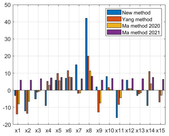
Yang et al. [25] defined the function score value as simply the total of lower and upper membership degrees of objects concerning each parameter. Ma et al. [44] applied Yang’s Algorithm 1, which is given in [25] to solve Example 2 and showed the score value as follows: $o_8⪰o_6⪰o_{14}⪰o_5⪰o_4⪰o_{10}⪰o_{12}⪰o_3⪰o_7⪰o_{13}⪰o_{15}⪰o_{11}⪰o_9⪰o_2⪰o_1.$

Ma et al. [44] proposed a new efficient decision-making algorithm by using added objects. By using Algorithm 3 Section 4 in [44], Example 2 was solved and the score value for all objects was obtained as follows $o_8⪰o_6⪰o_{14}⪰o_5⪰o_4⪰o_{10}⪰o_{12}⪰o_3⪰o_7⪰o_{13}⪰o_{15}⪰o_{11}⪰o_9⪰o_2⪰o_1.$

Ma et al. [43] applied a new decision-making algorithm, based on the average table and the antithesis table—the antithesis the table has symmetry between the objects. Applying Algorithm in [43], Section 3, to solve the Example 2, the following ranking of objects is obtained $o_8⪰o_6⪰o_5⪰o_{14}⪰o_4⪰o_{12}⪰o_{10}⪰o_3⪰o_{13}⪰o_7⪰o_{15}⪰o_{11}⪰o_2⪰o_9⪰o_1.$

The comparison results among the present method and methods in [25,43,44] are given in Figure 1.

Figure 1. Comparison methods.

Algorithm 1: Rangking Objects by Interval-Valued Fuzzy Soft Topology

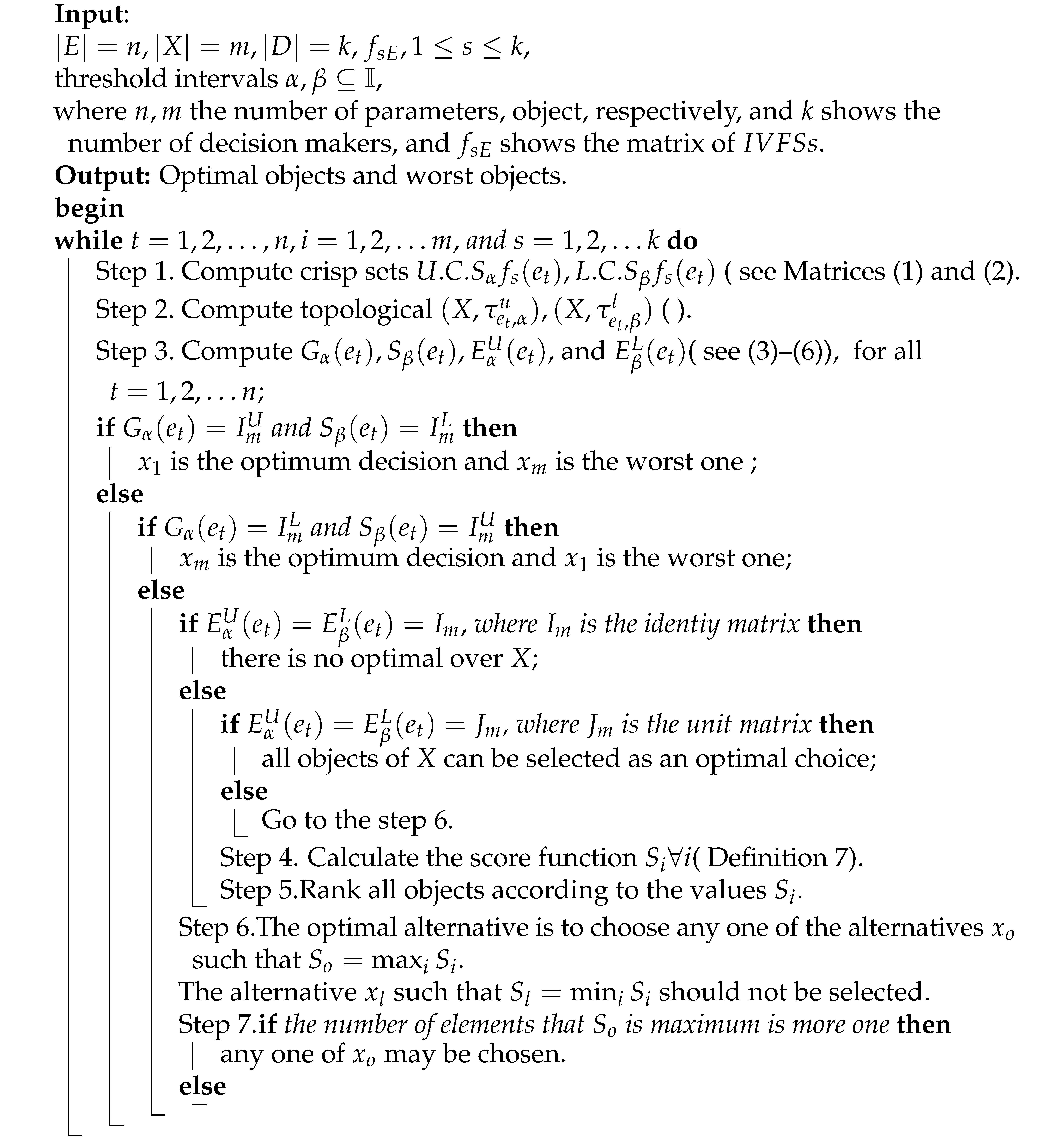5. Discussion

According to the present method and the methods proposed in [25,43,44], to reach the process consensus, Yang et al. [25] use the “AND” operator, while methods in [43,44] did not discuss the aggregation problem. In addition, Example 2 shows that all the methods have the same option $o_8$, which is the best object. Consequently, algorithms in methods [25,43,44] select just one option, which is the optimum, and do not select the worst option, while the proposed algorithm selects two options—the optimum and as well as the worst option. However, the methods in [25,43,44], rank the objects based on a linear ordering system (see Example 3), while the present method ranks the objects based on preorder relation and a preference relationship, which allows one to have some incomparable objects (nonlinear ordering system). For example, in the Example 2, the objects $o_{12}$ and $o_5$ have the same overall score values, which means that these objects cannot be compared with all of the others.

This is the same for the objects $o_{13}$, $o_1$ and $o_{14},$$o_4$ (see Figure 2). The comparison results between the new proposed method and methods in [25,43,44] are also given in Table 11.

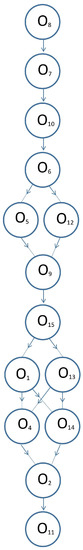
Figure 2. Nonlinear ordering system.

Table 11. Comparison of Existing Methods.

Methods	Output Comparision	Aggregation Methodology	Ranking Methodology	Rank the Objects
[25]	optimal option	AND operator	fuzzy choice values	a linear ordering system
[44]	optimal option	Not discussed	choice values	a linear ordering system
[43]	optimal option	Not discussed	score function computed from an average and an antithesis tables	a linear ordering system
present method	optimal option and worst	$IVFST$	A collective preference relationship in topological space	a nonlinear ordering system

6. Conclusions

The interval-valued soft set is a useful tool to deal with fuzziness and uncertainties in decision-making problems. In this paper, we constructed two crisp topological spaces over the set of objects, and then presented two different preorder relations in these topological spaces. By using a new method for ranking data, we proposed an approach for solving multi-attribute group decision-making problems by using a new method for ranking data. Finally, a real-life example has been presented to verify the proposed method approach and to demonstrate the effectiveness by comparing the results with those of some of the existing approaches.

For future research, it would be of merit to apply the decision-making methods into practical applications such as evaluation systems, recommender systems, and conflict handling.

References

- Zadeh, L.A. Fuzzy sets. Inf. Control 1965, 8, 338–353. [Google Scholar] [CrossRef] [Green Version]
- Gorzałczany, M.B. A method of inference in approximate reasoning based on interval-valued fuzzy sets. Fuzzy Sets Syst. 1987, 21, 1–17. [Google Scholar] [CrossRef]
- Atanassov, K.T. Intuitionistic fuzzy sets. In Intuitionistic Fuzzy Sets; Physica: Heidelberg, Germany, 1999; pp. 1–137. [Google Scholar]
- Pawlak, Z. Rough sets. Int. J. Comput. Inf. Sci. 1982, 11, 341–356. [Google Scholar] [CrossRef]
- Molodtsov, D. Soft set theory first results. Comput. Math. Appl. 1999, 37, 19–31. [Google Scholar] [CrossRef] [Green Version]
- Maji, P.K.; Biswas, P.; Roy, A.R. A fuzzy soft sets. J. Fuzzy Math. 2001, 9, 89–602. [Google Scholar]
- Roy, A.R.; Maji, P.K. A fuzzy soft set theoretic approach to decision making problems. J. Comput. Appl. Math. 2007, 203, 412–418. [Google Scholar] [CrossRef] [Green Version]
- Kong, Z.; Gao, L.; Wang, L. Comment on “A fuzzy soft set theoretic approach to decision making problems”. J. Comput. Appl. Math. 2009, 223, 540–542. [Google Scholar] [CrossRef] [Green Version]
- Feng, F.; Jun, Y.B.; Liu, X.; Li, L. An adjustable approach to fuzzy soft set based decision making. J. Comput. Appl. Math. 2010, 234, 10–20. [Google Scholar] [CrossRef] [Green Version]
- Alcantud, J.C.R. A novel algorithm for fuzzy soft set based decision making from multiobserver input parameter data set. Inf. Fusion 2016, 29, 142–148. [Google Scholar] [CrossRef]
- Alcantud, J.C.R. Some formal relationships among soft sets, fuzzy sets, and their extensions. Int. J. Approx. Reason. 2016, 68, 45–53. [Google Scholar] [CrossRef]
- Alcantud, J.C.R.; Mathew, T.J. Separable fuzzy soft sets and decision making with positive and negative attributes. Appl. Soft Comput. 2017, 59, 586–595. [Google Scholar] [CrossRef]
- Aktaş, H.; Çağman, N. Soft decision making methods based on fuzzy sets and soft sets. J. Intell. Fuzzy Syst. 2016, 30, 2797–2803. [Google Scholar] [CrossRef]
- Maji, P.K. More on intuitionistic fuzzy soft sets. In International Workshop on Rough Sets, Fuzzy Sets, Data Mining, and Granular-Soft Computing; Springer: Berlin/Heidelberg, Germany, 2009; pp. 231–240. [Google Scholar]
- Maji, P.K.; Biswas, R.; Roy, A.R. Intuitionistic fuzzy soft sets. J. Fuzzy Math. 2001, 9, 677–692. [Google Scholar]
- Jiang, Y.; Tang, Y.; Chen, Q.; Liu, H.; Tang, J. Interval-valued intuitionistic fuzzy soft sets and their properties. Comput. Math. Appl. 2010, 60, 906–918. [Google Scholar] [CrossRef] [Green Version]
- Maji, P.K.; Roy, A.R.; Biswas, R. On intuitionistic fuzzy soft sets. J. Fuzzy Math. 2004, 12, 669–684. [Google Scholar]
- Liu, Y.; Qin, K.; Martínez, L. Improving decision making approaches based on fuzzy soft sets and rough soft sets. Appl. Soft Comput. 2018, 65, 320–332. [Google Scholar] [CrossRef]
- Feng, F.; Li, C.; Davvaz, B.; Ali, M.I. Soft sets combined with fuzzy sets and rough sets: A tentative approach. Soft Comput. 2010, 14, 899–911. [Google Scholar] [CrossRef]
- Roy, S.; Samanta, T.K. A note on fuzzy soft topological spaces. Ann. Fuzzy Math. Inform. 2012, 3, 305–311. [Google Scholar]
- Tanay, B.; Kandemir, M.B. Topological structure of fuzzy soft sets. Comput. Math. Appl. 2011, 61, 2952–2957. [Google Scholar] [CrossRef] [Green Version]
- Khameneh, A.Z.; Kılıçman, A.; Salleh, A.R. Fuzzy soft boundary. Ann. Fuzzy Math. Inform. 2014, 8, 687–703. [Google Scholar]
- Khameneh, A.Z.; Kılıçman, A.; Salleh, A.R. Fuzzy soft product topology. Ann. Fuzzy Math. Inform. 2014, 7, 935–947. [Google Scholar]
- Son, M.-J. Interval-valued Fuzzy Soft Sets. J. Korean Inst. Intell. Syst. 2007, 17, 557–562. [Google Scholar] [CrossRef] [Green Version]
- Yang, X.; Lin, T.Y.; Yang, J.; Li, Y.; Yu, D. Combination of interval-valued fuzzy set and soft set. Comput. Math. Appl. 2009, 58, 521–527. [Google Scholar] [CrossRef] [Green Version]
- Feng, F.; Li, Y.; Leoreanu-Fotea, V. Application of level soft sets in decision making based on interval-valued fuzzy soft sets. Comput. Math. Appl. 2010, 60, 1756–1767. [Google Scholar] [CrossRef] [Green Version]
- Xiao, Z.; Chen, W.; Li, L. A method based on interval-valued fuzzy soft set for multi-attribute group decision-making problems under uncertain environment. Knowl. Inf. Syst. 2013, 34, 653–669. [Google Scholar] [CrossRef]
- Khameneh, A.Z.; Kılıçman, A.; Salleh, A.R. An adjustable approach to multi-criteria group decision-making based on a preference relationship under fuzzy soft information. Int. J. Fuzzy Syst. 2017, 19, 1840–1865. [Google Scholar] [CrossRef]
- Khameneh, A.Z.; Kılıçman, A.; Salleh, A.R. Application of a preference relationship in decision-making based on intuitionistic fuzzy soft sets. J. Intell. Fuzzy Syst. 2018, 34, 123–139. [Google Scholar] [CrossRef]
- Khameneh, A.Z.; Kılıçman, A.; Salleh, A.R. An adjustable method for data ranking based on fuzzy soft sets. Indian J. Sci. Technol. 2015, 8, 1–9. [Google Scholar]
- Jiang, Y.; Tang, Y.; Liu, H.; Chen, Z. Entropy on intuitionistic fuzzy soft sets and on interval-valued fuzzy soft sets. Inf. Sci. 2013, 240, 95–114. [Google Scholar] [CrossRef]
- Turksen, I.B.; Zhong, Z. An approximate analogical reasoning schema based on similarity measures and interval-valued fuzzy sets. Fuzzy Sets Syst. 1990, 34, 323–346. [Google Scholar] [CrossRef]
- Peng, X.; Yang, Y. Algorithms for interval-valued fuzzy soft sets in stochastic multi-criteria decision making based on regret theory and prospect theory with combined weight. Appl. Soft Comput. 2017, 54, 415–430. [Google Scholar] [CrossRef]
- Peng, X.D.; Yang, Y. Information measures for interval-valued fuzzy soft sets and their clustering algorithm. J. Comput. Appl. 2015, 35, 2350–2354. [Google Scholar]
- Chen, W.J.; Zou, Y. Rational decision making models with incomplete information based on interval-valued fuzzy soft sets. J. Comput. 2017, 28, 193–207. [Google Scholar]
- Yuan, F.; Hu, M.J. Application of interval-valued fuzzy soft sets in evaluation of teaching quality. J. Hunan Inst. Sci. Technol. 2012, 25, 28–30. [Google Scholar]
- Esposito, C.; Moscato, V.; Sperlí, G. Trustworthiness Assessment of Users in Social Reviewing Systems. IEEE Trans. Syst. Man Cybern. Syst. 2021. [Google Scholar] [CrossRef]
- Han, Q.; Molinaro, C.; Picariello, A.; Sperli, G.; Subrahmanian, V.S.; Xiong, Y. Generating Fake Documents using Probabilistic Logic Graphs. IEEE Trans. Dependable Secur. Comput. 2021. [Google Scholar] [CrossRef]
- Rajarajeswari, P.; Dhanalakshmi, P. Interval-valued fuzzy soft matrix theory. Ann. Pure Appl. Math. 2014, 7, 61–72. [Google Scholar]
- Basu, T.M.; Mahapatra, N.K.; Mondal, S.K. Matrices in interval-valued fuzzy soft set theory and their application. S. Asian J. Math. 2014, 4, 1–22. [Google Scholar]
- Zhang, Q.; Sun, D. An Improved Decision-Making Approach Based on Interval-valued Fuzzy Soft Set. J. Phys. Conf. Ser. 2021, 1828, 012041. [Google Scholar] [CrossRef]
- Ma, X.; Qin, H.; Sulaiman, N.; Herawan, T.; Abawajy, J.H. The parameter reduction of the interval-valued fuzzy soft sets and its related algorithms. IEEE Trans. Fuzzy Syst. 2013, 22, 57–71. [Google Scholar] [CrossRef]
- Ma, X.; Wang, Y.; Qin, H.; Wang, J. A Decision-Making Algorithm Based on the Average Table and Antitheses Table for Interval-Valued Fuzzy Soft Set. Symmetry 2020, 12, 1131. [Google Scholar] [CrossRef]
- Ma, X.; Fei, Q.; Qin, H.; Li, H.; Chen, W. A new efficient decision making algorithm based on interval-valued fuzzy soft set. Appl. Intell. 2021, 51, 3226–3240. [Google Scholar] [CrossRef]
- Peng, X.; Garg, H. Algorithms for interval-valued fuzzy soft sets in emergency decision making based on WDBA and CODAS with new information measure. Comput. Ind. Eng. 2018, 119, 439–452. [Google Scholar] [CrossRef] [PubMed]
- Ali, M.; Kılıçman, A.; Khameneh, A.Z. Separation Axioms of Interval-Valued Fuzzy Soft Topology via Quasi-Neighborhood Structure. Mathematics 2020, 8, 178. [Google Scholar] [CrossRef] [Green Version]
- Lai, H.; Zhang, D. Fuzzy preorder and fuzzy topology. Fuzzy Sets Syst. 2006, 157, 1865–1885. [Google Scholar] [CrossRef]
Publisher’s Note: MDPI stays neutral with regard to jurisdictional claims in published maps and institutional affiliations. |
© 2021 by the authors. Licensee MDPI, Basel, Switzerland. This article is an open access article distributed under the terms and conditions of the Creative Commons Attribution (CC BY) license (https://creativecommons.org/licenses/by/4.0/).