Infinitely Smooth Polyharmonic RBF Collocation Method for Numerical Solution of Elliptic PDEs

Abstract

In this article, a novel infinitely smooth polyharmonic radial basis function (PRBF) collocation method for solving elliptic partial differential equations (PDEs) is presented. The PRBF with natural logarithm is a piecewise smooth function in the conventional radial basis function collocation method for solving governing equations. We converted the piecewise smooth PRBF into an infinitely smooth PRBF using source points collocated outside the domain to ensure that the radial distance was always greater than zero to avoid the singularity of the conventional PRBF. Accordingly, the PRBF and its derivatives in the governing PDEs were always continuous. The seismic wave propagation problem, groundwater flow problem, unsaturated flow problem, and groundwater contamination problem were investigated to reveal the robustness of the proposed PRBF. Comparisons of the conventional PRBF with the proposed method were carried out as well. The results illustrate that the proposed approach could provide more accurate solutions for solving PDEs than the conventional PRBF, even with the optimal order. Furthermore, we also demonstrated that techniques designed to deal with the singularity in the original piecewise smooth PRBF are no longer required.

1. Introduction

A large number of multidisciplinary problems may require solutions involving complicated mathematical models and numerical techniques [1,2]. Among these approaches, the meshfree method has gained the attention of researchers from different scientific fields due to its capability of dealing with partial differential equations (PDEs) with complicated and irregular geometry [3,4,5,6,7]. The radial basis function collocation method (RBFCM) is one meshfree approach for analyzing governing equations, where the unknowns are represented by a function approximation [8,9,10]. The RBFCM is also capable of solving linear and nonlinear PDEs requiring solutions involveing sophisticated mathematical models and numerical algorithms [8,9]. Function approximation using the interpolation method of the radial basis function (RBF) was proposed in 1971 by Hardy [11], who used the multiquadric (MQ) RBF for scattered data interpolation to solve problems. In addition to the MQ RBF, several RBFs may be found, such as the inverse multiquadric (IMQ), Gaussian, and polyharmonic spline (PS) functions [12,13,14]. Among them, the PS and the MQ RBFs may provide much more accurate solutions than other RBFs [15,16]. The RBFs are usually categorized into piecewise and infinitely smooth functions for solving PDEs in the RBFCM. For example, the PS is piecewise smooth. On the other hand, the MQ is infinitely smooth, with the shape parameter [17,18]. For the PS, a minimum order of two must be adopted to keep it smooth for solving Laplace-type equations [19]. Despite the great success of the above RBFs as effective numerical techniques for dealing with several kinds of PDEs, there is still growing interest in the application and development of new and advanced RBFs [20]. A significant number of modifications to RBFs have been proposed, such as the pseudo-spectral RBF [21,22], Gaussian RBF [23], RBF QR alternative basis method [24], finite difference RBF [25,26], partition of unity RBF [27,28], stabilized expansion of the Gaussian RBF [29], rational RBF [30,31], and RBF based on partition of unity of Taylor series expansion [32].

An adaptive greedy technique for the Kansa method is adopted for general PDE problems to be solved on complicated domains [5]. The adaptive greedy algorithm prefers exterior centers for large scaling parameters. Similar to the idea of exterior centers, Ku et al. presented a fictitious source collocation scheme where the centers are replaced by fictitious sources collocated outside the domain as well [33,34]. However, different from the greedy algorithm, the role of fictitious sources is emphasized on the prevention of singularity without the shape parameter for the MQ. Since the distance between the source and the interior point is always greater than zero, the MQ and its derivatives are always smooth and globally infinitely differentiable without using the shape parameter.

Motivated by this concept, a novel infinitely smooth polyharmonic radial basis function (PRBF) collocation method for solving elliptic partial differential equations (PDEs) is presented. The seismic wave propagation problem, groundwater flow problem, unsaturated flow problem, and groundwater contamination problem were investigated to reveal the robustness of the proposed PRBF. Comparisons of the conventional PRBF with the proposed method were carried out as well. The formulation of the PRBF is introduced in Section 2. The convergence analysis is presented in Section 3. Section 4 details the results of the investigation into the geomechanical problems listed above. The findings of this research are finally summarized in Section 5.

2. The Polyharmonic Radial Basis Function Collocation Method

2.1. The Governing Equation

The governing equation for elliptic partial differential equations in two dimensions can be expressed as

$${\nabla }^{2}u(x)+A\cdot \nabla u(x)+Bu(x)=C(x) \mathrm{in} \Omega$$

(1)

$$u(x)=g(x)\mathrm{on}\partial \Omega$$

(2)

where $\nabla$ denotes the divergence operator; $\cdot$ denotes the dot product; $u(x)$ denotes the unknown, $x=(x,y)$; $\Omega$ denotes a domain with the boundary $\partial \Omega$; $g(x)$ denotes the boundary value; $A$ is the velocity in two dimensions, $A=\left(A_x,A_y\right)$; B is the given function; and $C(x)$ is the given function value.

In the RBFCM, several RBFs can be implemented, such as the MQ, Gaussian, IMQ, and PS functions. However, the accuracy of the Gaussian, MQ, and IMQ RBFs may depend on the shape parameter. Thus, most applications of the Gaussian, MQ, and IMQ RBFs utilize optimization approaches or experimental techniques to determine the optimal shape parameter [17,18]. Since the PS may provide good agreement without providing an additional parameter to prevent singularity, we considered the PRBF in this study. The PRBF with natural logarithm is defined as

$$\phi (r)=r_{}^{2k}\ln (r),k=1,2,3\dots$$

(3)

where k is the order; $r$ is the radial distance, $r=\left|x-x^s\right|$; $x$ denotes the interior point; and $x^s$ denotes the center point. The equation is a kth order PRBF.

Taking the derivative of (3) with respect to x gives

$$\frac{\partial \phi (r)}{\partial x}=(x-x^s)r_{}^{2k-2}[2k\ln (r)+1]$$

(4)

where $x^s$ is the x-coordinate of the center point. We may then take the derivative of y and obtain

$$\frac{\partial \phi (r)}{\partial y}=(y-y^s)r_{}{}^{2k-2}[2k\ln (r)+1]$$

(5)

where $y^s$ is the y-coordinate of the center point. Similarly, we have

$$\frac{{\partial }^2\phi (r)}{\partial x^2}={(x-x^s)}^2{r}_{}{}^{2k-4}\left[\right(4k^2-4k)\ln r+4k-2]+r_{}{}^{2k-2}[2k\ln (r)+1].$$

(6)

Again, we take the derivative of y and obtain

$$\frac{{\partial }^2\phi (r)}{\partial y^2}={(y-y^s)}^2{r}_{}{}^{2k-4}\left[\right(4k^2-4k)\ln r+4k-2]+r_{}{}^{2k-2}[2k\ln (r)+1].$$

(7)

Utilizing the PRBF to build up the function approximation, we obtain

$$u(x)={\displaystyle \sum _{j=1}^{n_c}{\lambda }_j\phi (r_j)}$$

(8)

where $n_c$ denotes the total number of center points; ${\lambda }_j$ denotes the unknown coefficient; $\phi (r_j)$ denotes the basis function; $r_j$ is the radial distance at the jth center point, $r_j=\left|x-x_j^s\right|$; and $x_j^s$ denotes the jth center point, described as $x_j^s=(x_j^s,y_j^s)$.

Inserting the aforementioned equations into (1), the function approximation of the governing equation is as follows:

$$\begin{array}{l}{\displaystyle \sum _{j=1}^{n_c}{\lambda }_j{r}_j{}^{2k-2}(4k^2\ln r_j+4k)}\\ +{\displaystyle \sum _{j=1}^{n_c}{\lambda }_j[A_x(x-x_j^s)+A_y(y-y_j^s)]r_j{}^{2k-2}[2k\ln (r_j)+1]}+{\displaystyle \sum _{j=1}^{n_c}{\lambda }_{j}B{r}_j^{2k}\ln \left(r_j\right)}=C(x).\end{array}$$

(9)

From (9), it is clear that $\ln (r_j)$ becomes singular when $r_j^{}=0$, where the position of the center point exactly coincides with the position of the interior point. In this study, we propose a novel idea to convert the piecewise smooth PRBF into an infinitely smooth PRBF using source points collocated outside the domain to ensure that the radial distance is always greater than zero, thus avoiding the singularity of the conventional PRBF. Accordingly, the terms in (9) are always smooth, and no extra techniques are required to deal with the singularity. The concept of fictitious sources is elaborated in the following section.

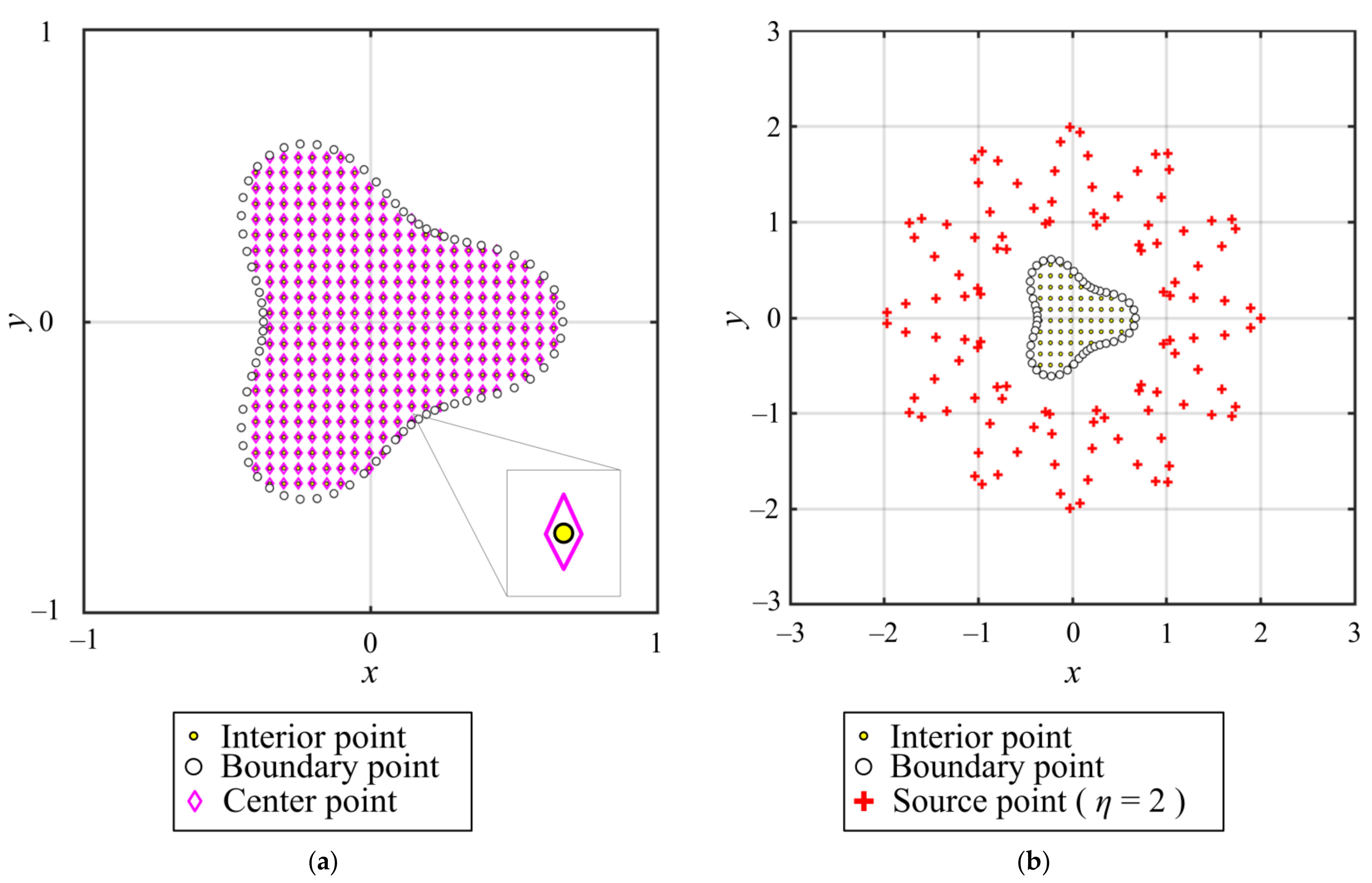
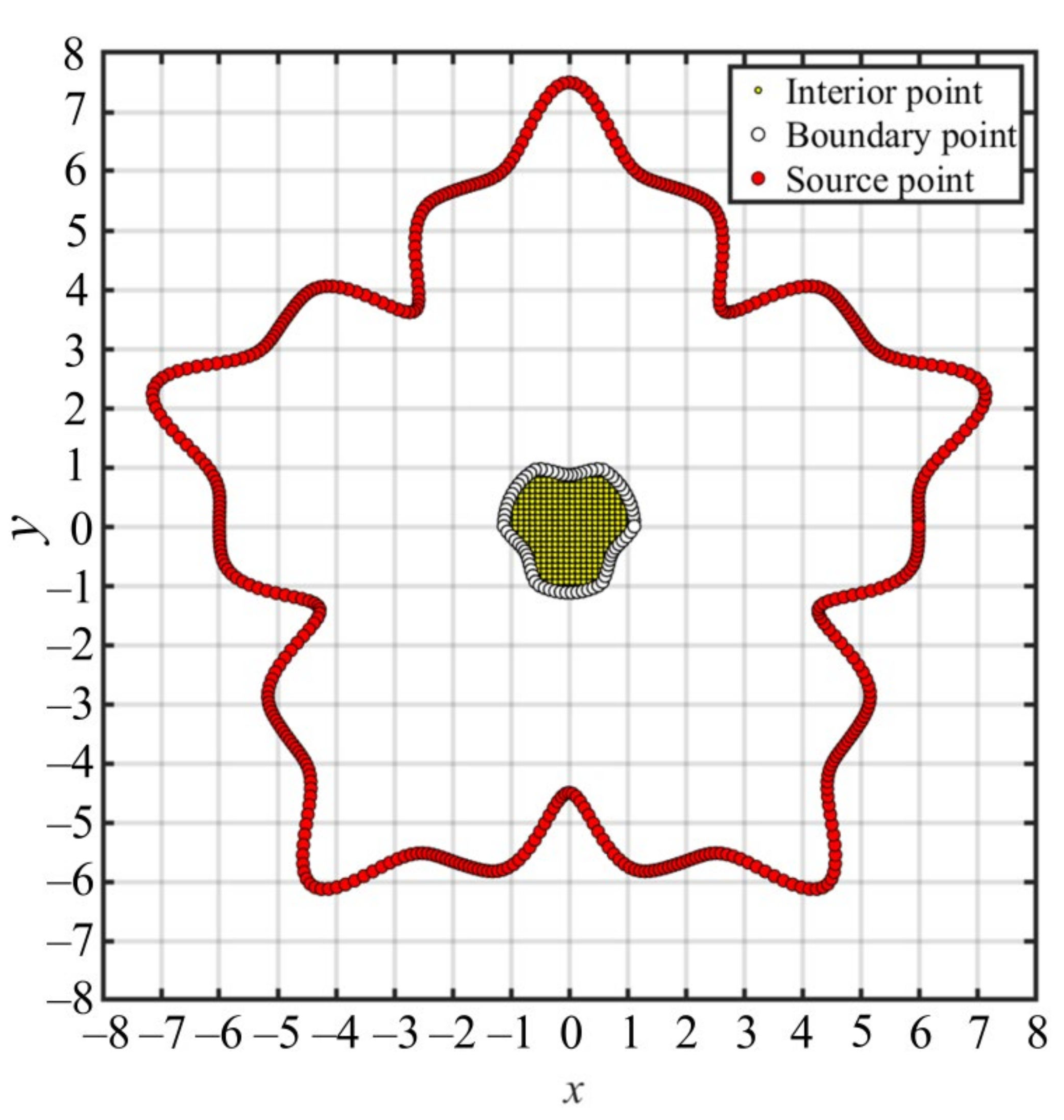
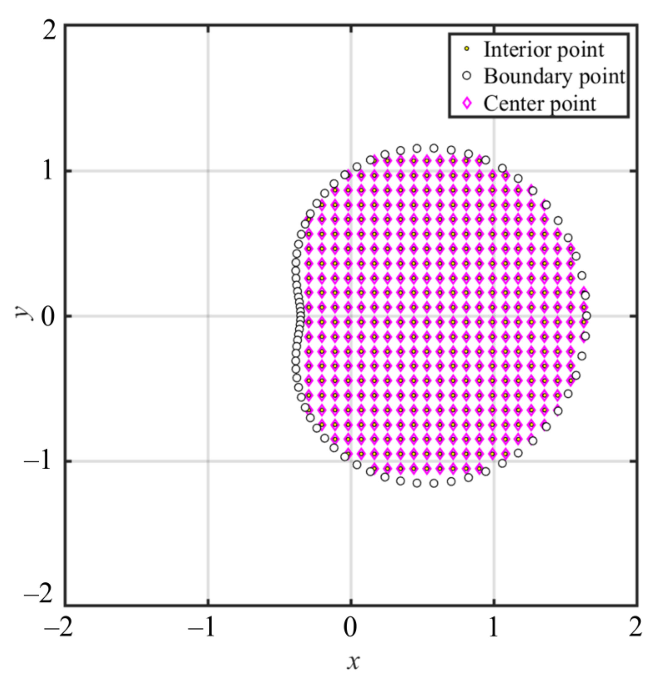
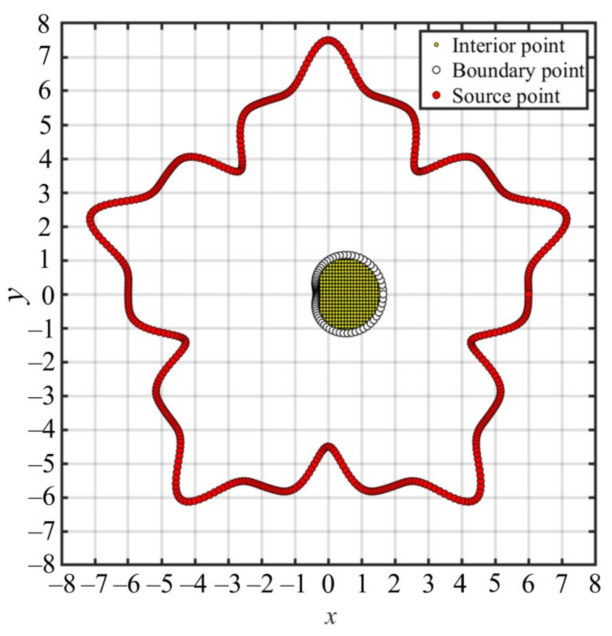
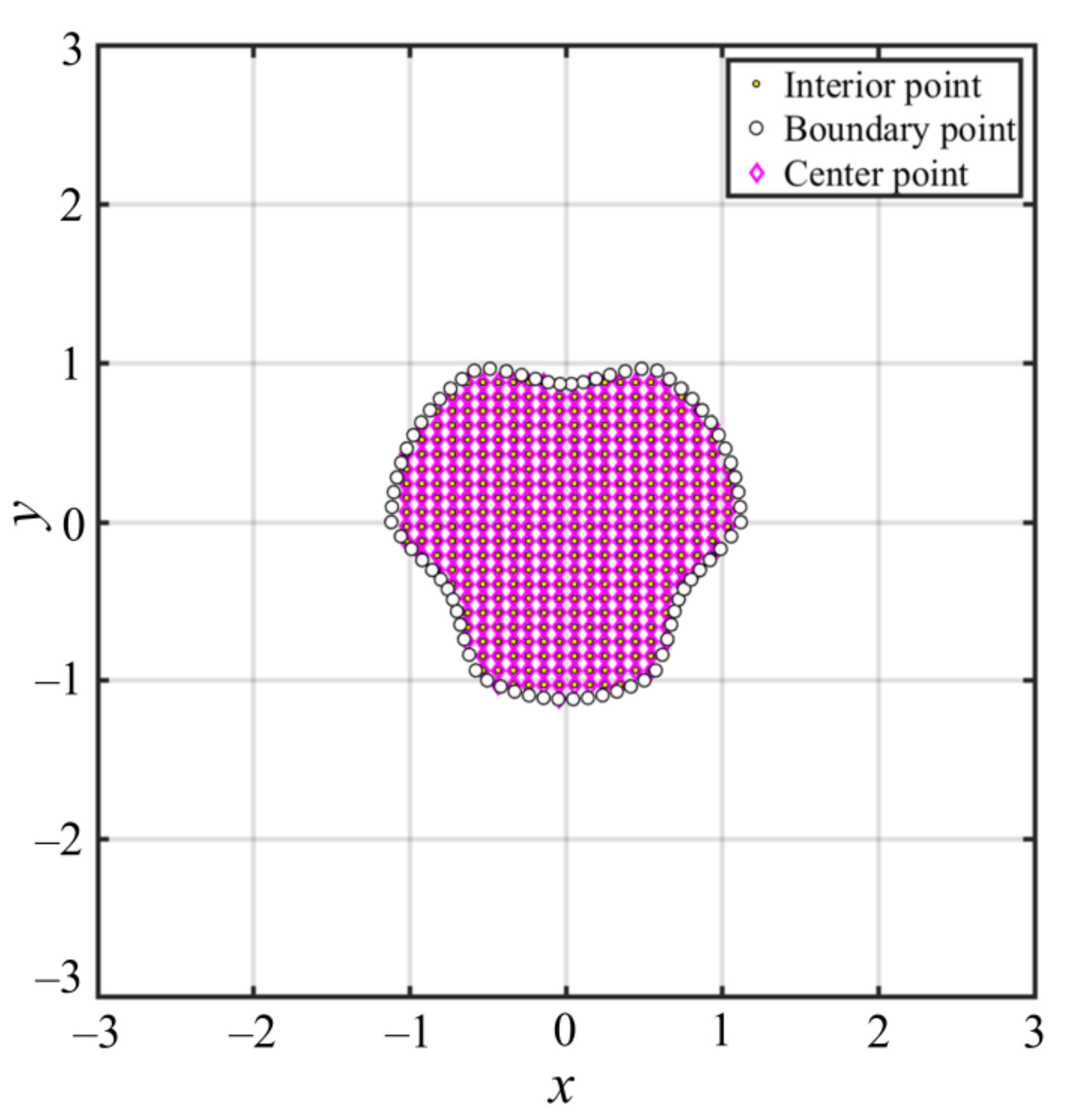
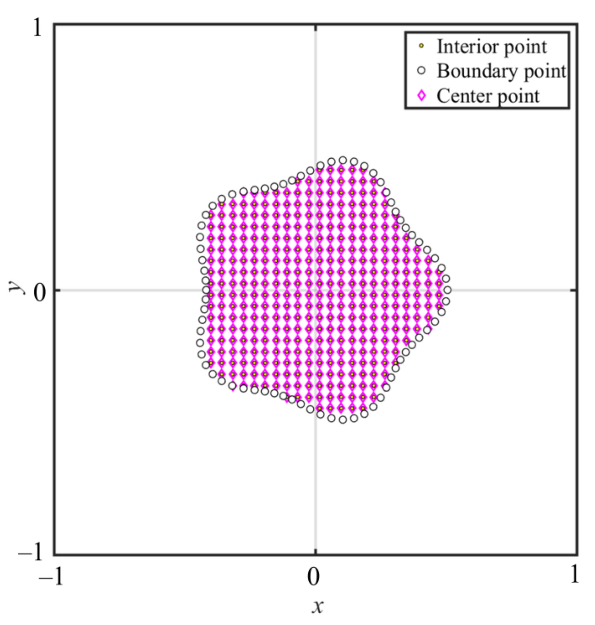
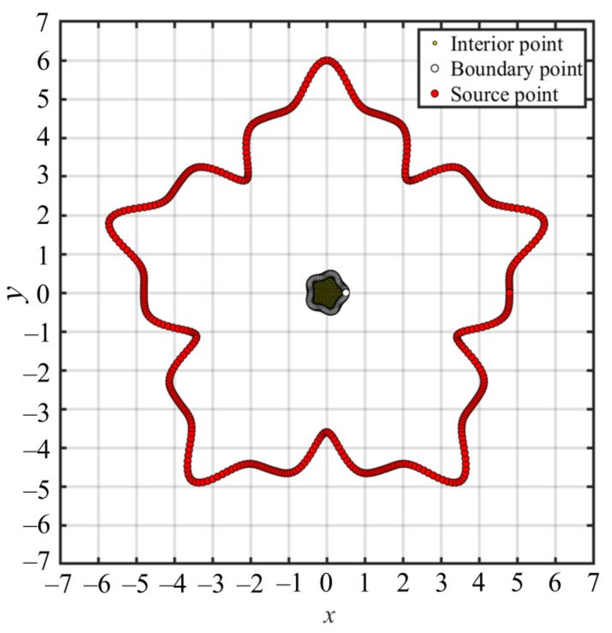
2.2. The Fictitious Sources

In the conventional PRBF, the interior, center, and boundary points have to be placed where the positions of the interior and center points are usually the same, as displayed in Figure 1a. To prevent singularity, the PRBF with natural logarithm is usually implemented as follows [15]:

$$\phi (r)=r_{}^{2k-1}\ln (r^r),k=1,2,3\dots .$$

(10)

Using (8), we may obtain the function approximation for the governing equation again

$$\begin{array}{l}{\displaystyle \sum _{j=1}^{n_s}{\lambda }_j{r}_j{}^{2k-3}[4k^2\ln (r_j{}^{r_j})+4k{r}_j]}\\ +{\displaystyle \sum _{j=1}^{n_s}{\lambda }_j[A_x(x-x_j^s)+A_y(y-y_j^s)]r_j{}^{2k-3}[2k\ln (r_j{}^{r_j})+r_j]}+{\displaystyle \sum _{j=1}^{n_s}{\lambda }_{j}B{r}_j^{2k-1}\ln (r_j{}^{r_j})}=C(x).\end{array}$$

(11)

where $n_s$ denotes the number of fictitious sources. To prevent singularity, a minimum order of two must be utilized to ensure that $r_j^{2k-3}$ in the above equation is a smooth and completely monotone RBF. Accordingly, the PRBF with natural logarithm is a piecewise smooth function in the conventional RBFCM.

In this study, fictitious sources are adopted. The center points in the PRBF are regarded as the fictitious sources, where the fictitious sources are placed outside the domain, as depicted in Figure 1b.

The following equation is utilized for placing the source points.

$${\mathbf{x}}_j^s=(\eta {\rho }_j^s\cos {\theta }_j^s,\eta {\rho }_j^s\sin {\theta }_j^s),j=1,\dots ,n_s$$

(12)

where $\eta$ denotes the dilation parameter; ${\rho }_j^s$ denotes the radius of the fictitious sources at the jth source point; and ${\theta }_j^s$ denotes the angle of the fictitious sources at the jth source point. Figure 1b depicts the proposed fictitious sources. As shown in Figure 1b, the positions of the source points can, therefore, be collocated with the consideration of different values of the dilation parameter by utilizing (12). Since the radial distance is always nonzero, the PRBF and its derivatives in the governing equation, as depicted in (3) and (9), are always continuous. Based on the proposed fictitious sources, the original piecewise smooth PRBF is then converted into an infinitely smooth PRBF.

To investigate the unknown coefficients, approximations are applied to satisfy (1) with the boundary conditions, as shown in (2), at each point. The following linear system is acquired:

$$\left[\begin{array}{c}{[{\mathbf{A}}_L]}_{n_i\times n_s}\\ {[{\mathbf{A}}_B]}_{n_b\times n_s}\end{array}\right]\left[\mathsf{\lambda }\right]=\left[\begin{array}{c}{[f]}_{n_i\times 1}\\ {[g]}_{n_b\times 1}\end{array}\right]$$

(13)

where $A_L$ denotes a $n_i\times n_s$ matrix for the interior points; $A_B$ denotes a $n_b\times n_s$ matrix for the boundary points; $\mathsf{\lambda }$ denotes a $n_s\times 1$ vector which includes unknown coefficients ${\lambda }_j$ to be solved; $f$ denotes a $n_i\times 1$ vector of function values for the interior points, written as $f=[C_1,C_2,\dots ,C_{n_i}]$; $g$ denotes an $n_b\times 1$ vector of boundary data, written as $g=[g_1,g_2,\dots ,g_{n_b}]$; $n_i$ denotes the number of interior points; and $n_b$ denotes the number of boundary points. The undetermined coefficients can be obtained by solving a system of simultaneous linear equations in matrix form as shown in (13).

Accordingly, the solution of $u\left(x\right)$ can be obtained using the function approximation of (8). To evaluate the error, the root-mean-square error (RMSE) and the maximum absolute error (MAE) are both adopted. The accuracy of the computed results is compared to the exact solutions using the following equations.

$$\mathrm{RMSE}=\sqrt{\frac{{\displaystyle \sum _{i=1}^I{(u_E(x_i)-u(x_i))}^2}}{I}},$$

(14)

$$\mathrm{MAE}=\mathrm{maximum}\left|u_E\left(x_i\right)-u\left(x_i\right)\right|,1\le i\le I$$

(15)

where I is the total number of interior points, RMSE is the root-mean-square error, MAE is the maximum absolute error, and $u(x_i)$ and $u_E(x_i)$ represent the numerical and exact solutions at the ith interior point, respectively.

3. Convergence Analysis

To compare the proposed PRBF with the conventional PRBF, we firstly consider a steady-state groundwater flow problem [33]:

$${\nabla }^{2}u(\mathbf{x})=0.$$

(16)

An irregular boundary was defined as

$$\begin{array}{l}\partial \Omega =\left\{(x,y)\left|x=\rho (\theta )\cos \theta ,y=\rho (\theta )\sin \theta \right.\right\},\\ \rho (\theta )={[\cos (3\theta )+\sqrt{2-{\sin }^2(3\theta )}]}^{1/3},0\le \theta \le 2\pi .\end{array}$$

(17)

The boundary data, as depicted in (18), were assigned on the irregular boundaries.

$$g(x)=e^y\sin (x)+e^x\cos (y).$$

(18)

We used 321 interior points, 396 fictitious sources, and 75 boundary points. In this example, we consider six cases with different shapes of fictitious sources using (19) to (24) as demonstrated in Figure 2a–f for Cases I, II, III, IV, V, and VI, respectively.

$${\rho }_{j_1}^s({\theta }_j^s)={[\cos (3{\theta }_j^s)+\sqrt{2-{\sin }^2(3{\theta }_j^s)}]}^{1/3},0\le {\theta }_j^s\le 2\pi ,$$

(19)

$${\rho }_{j_2}^s({\theta }_j^s)=e^{{(\sin {\theta }_j^s\sin 2{\theta }_j^s)}^2}+e^{{(\cos {\theta }_j^s\cos 2{\theta }_j^s)}^2},0\le {\theta }_j^s\le 2\pi ,$$

(20)

$${\rho }_{j_3}^s({\theta }_j^s)=1+{\cos }^2(6{\theta }_j^s),0\le {\theta }_j^s\le 2\pi ,$$

(21)

$${\rho }_{j_4}^s({\theta }_j^s)=1+{\sin }^4(2{\theta }_j^s),0\le {\theta }_j^s\le 2\pi ,$$

(22)

$${\rho }_{j_5}^s({\theta }_j^s)=6-{\cos }^4(4{\theta }_j^s),0\le {\theta }_j^s\le 2\pi ,$$

(23)

$${\rho }_{j_6}^s({\theta }_j^s)=4+{\sin }^5(5{\theta }_j^s),0\le {\theta }_j^s\le 2\pi .$$

(24)

The fictitious sources were placed on the external domain by utilizing (25). The fictitious source boundaries were defined as [33,34]

$$\partial {\Omega }^s=\left\{(x_j^s,y_j^s)\left|x_j^s=\eta {\rho }_j^s\cos {\theta }_j^s,y_j^s=\eta {\rho }_j^s\sin {\theta }_j^s\right.\right\}$$

(25)

where $\partial {\Omega }^s$ denotes the boundaries of fictitious sources. Figure 3 illustrates the MAE values of the conventional and proposed PRBFs with different orders (values of k). In Case I, the MAE tended to increase with an increase in the order k, as displayed in Figure 3a. In the other five cases, it was found that the MAE of the proposed PRBF remained lower than that of the conventional one with different orders, as displayed in Figure 3b–f. The accuracy is less sensitive to the order k. From Figure 3, accurate results with order k in the range of one to ten were acquired. Additionally, the results demonstrate that the proposed PRBF with an order of one provides more accurate results than the conventional one, as depicted in

Table 1. A comparison of the results.

		Optimum Order	Dilation Parameter	MAE	RMSE
The conventional PRBF		7	-	$5.87\times {10}^{-4}$	$8.21\times {10}^{-6}$
The proposed method	Case I	1	5	$8.91\times {10}^{-7}$	$2.14\times {10}^{-8}$
	Case II	1	5	$2.51\times {10}^{-10}$	$5.04\times {10}^{-12}$
	Case III	1	5	$3.03\times {10}^{-12}$	$4.95\times {10}^{-14}$
	Case IV	1	5	$2.66\times {10}^{-10}$	$4.35\times {10}^{-12}$
	Case V	1	5	$5.13\times {10}^{-9}$	$8.98\times {10}^{-11}$
	Case VI	1	5	$6.65\times {10}^{-8}$	$1.48\times {10}^{-9}$

. The MAE of the conventional PRBF was in the order of ${10}^{-1}$ to ${10}^{-4}$ as the order k ranged from two to ten. It appears that the MAE for the conventional PRBF could only reach the order of ${10}^{-4}$ when the order k was set to seven, as displayed in Figure 3.

The MAE of the proposed PRBF with different dilation parameters was investigated, as displayed in Figure 4. In Cases I, II, III, and IV, the MAE declined with an increase in the dilation parameters—thus, all cases could obtain accurate results. As depicted in Figure 4e,f these results show that accurate results in the order of ${10}^{-6}$ to ${10}^{-11}$ were yielded when an arbitrary dilation parameter in the range of zero to ten was utilized.

It is found that the error may grow with the increase of the dilation parameter. However, results from all cases reveal that we may obtain accurate results with the use of an arbitrary value in the range of 1.5 to 5 for the dilation parameter. Nevertheless, the error may increase while the larger dilation parameter is adopted. However, it reveals that we could still obtain better accuracy than original PS even in the worst case.

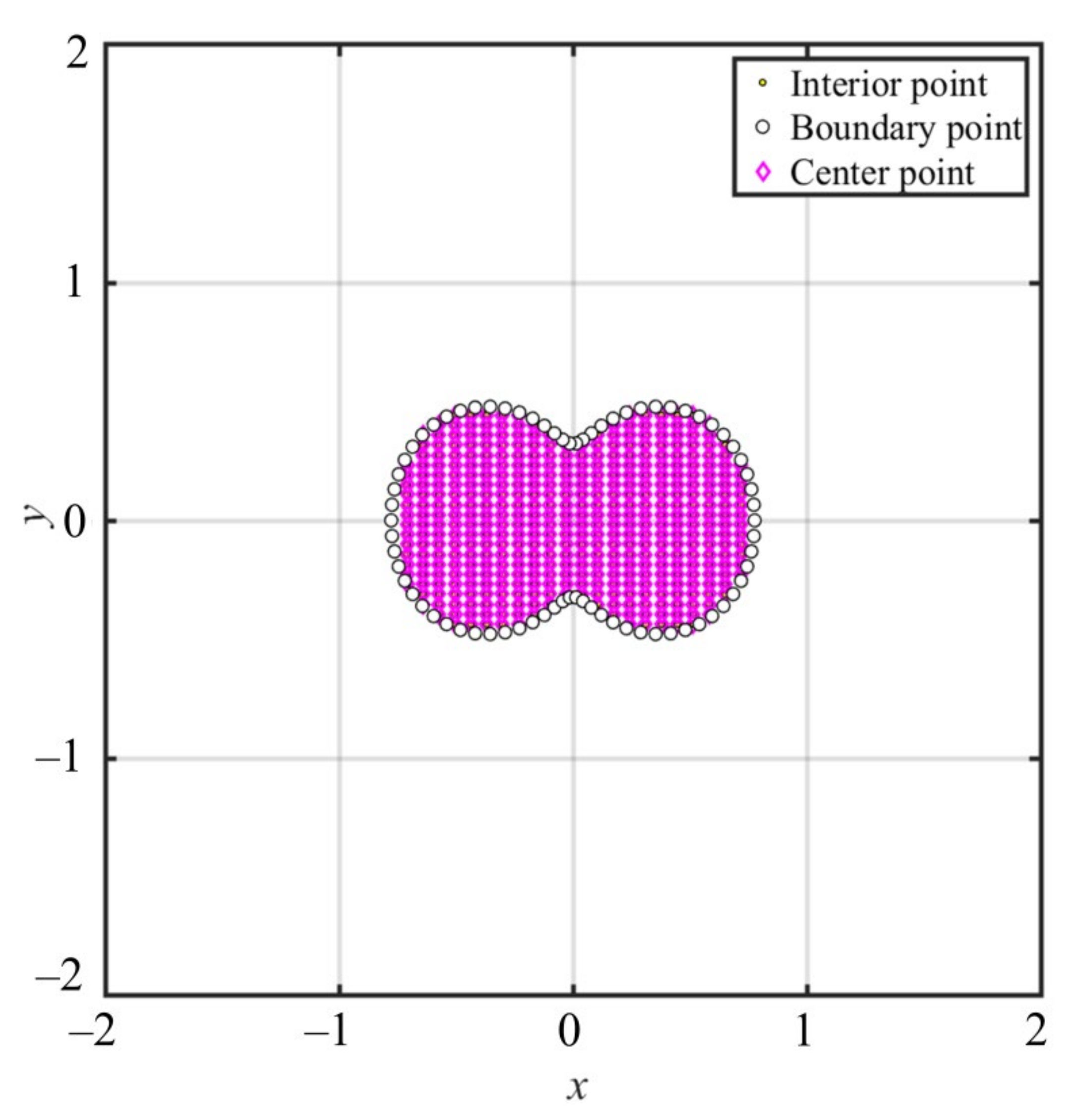
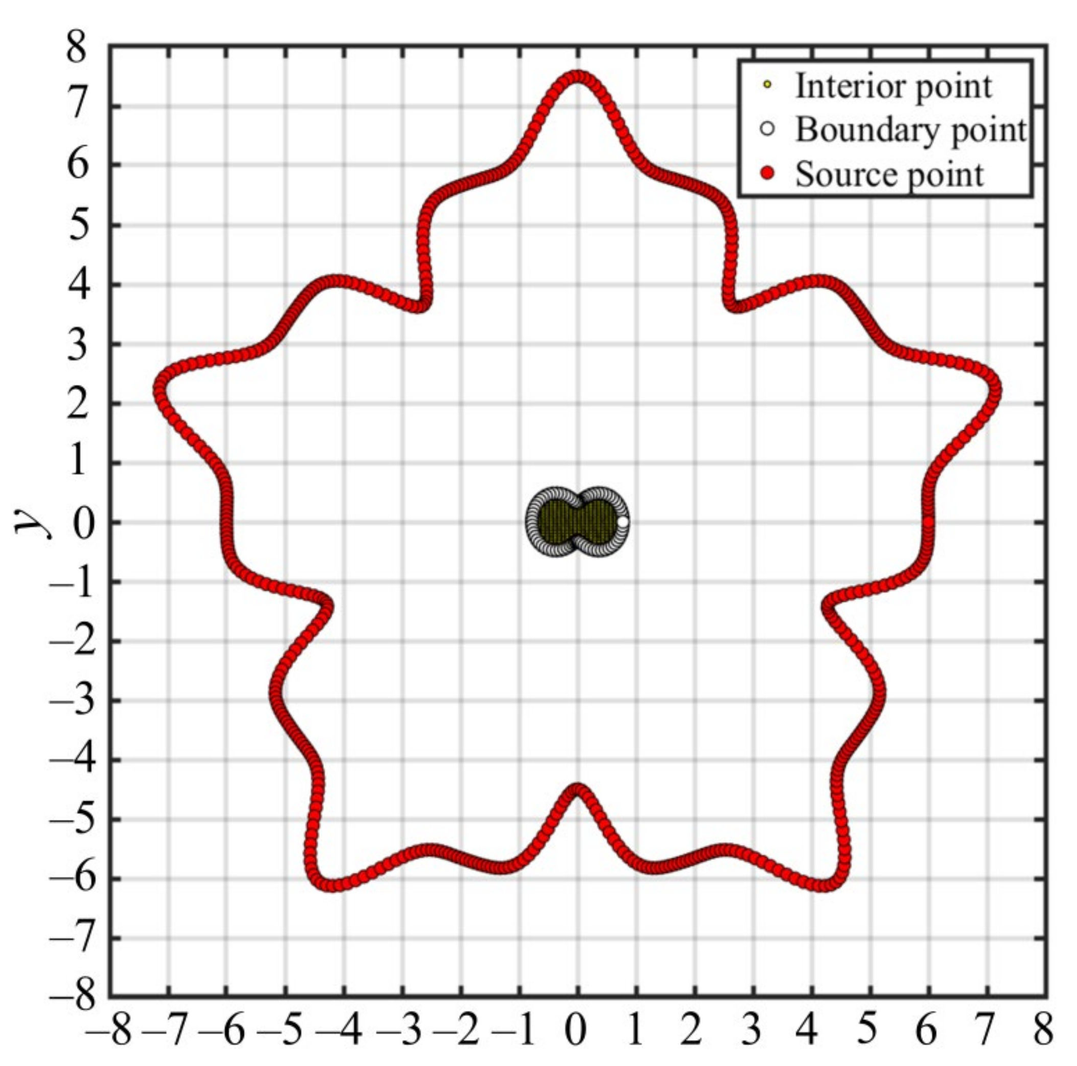
4. Numerical Examples

To demonstrate the applicability of the proposed method, several types of geomechanical problems—the seismic wave propagation problem, groundwater flow problem, unsaturated flow problem, and groundwater contamination problem—were investigated; the results are presented in this section.

4.1. The Seismic Wave Propagation Problem

The problem of seismic wave propagation [35] is considered as

$$({\nabla }^2-{\lambda }^2)u(x,y)=0$$

(26)

where ${\lambda }^2$ denotes the wave number depending on the property of the geomaterial. The boundary is

$$\partial \Omega =\left\{(x,y)\left|x=\rho (\theta )\cos \theta ,y=\rho (\theta )\sin \theta \right.\right\},\rho (\theta )=2+1.3\cos (\theta ),0\le \theta \le 2\pi .$$

(27)

Data are assigned on the boundaries by the exact solution:

$$g(\mathrm{x})=e^{(\lambda /2)(x+\sqrt{3}y)}.$$

(28)

In this wave problem, we assigned ${\lambda }^2=1$ and ${\lambda }^2=0.0001$. The conventional PRBF and the proposed PRBF with fictitious sources were utilized to solve this problem. In the conventional PS RBF, the order $k\ge 2$ was adopted to prevent the singularity. In the proposed PRBF with fictitious sources, the irregular boundaries of the exterior sources, $\partial {\Omega }_s$, defined by (24), were utilized in this example. Figure 5 shows the original collocation points for the conventional case. We used 480 center points and 75 boundary points. For the fictitious sources, demonstrated in Figure 6, the interior points, boundary points, and fictitious sources were placed within, on, and outside the region, respectively. The numbers of source, boundary, and interior points were 480, 75, and 405, respectively.

Figure 7a shows the order k versus the MAE when the wave number was 0.0001. From Figure 7a, the MAE of the conventional PRBF fluctuated between ${10}^{-1}$ and ${10}^{-4}$ as the order k ranged from two to ten. It appears that the proposed approach with order of one acquired the most accurate results, with MAE in the order of ${10}^{-13}$—much better than the conventional PS RBF. Figure 7b shows the order k versus the MAE when the wave number was 1. From Figure 7b, the MAE of the conventional PS RBF fluctuated between ${10}^{-1}$ and ${10}^{-4}$ as the order k ranged from two to ten. However, the MAE of the proposed PRBF utilizing fictitious sources drastically decreased from ${10}^2$ to ${10}^{-10}$ as the order k ranged from one to ten. It is clear that the proposed PRBF with fictitious sources can provide significantly more accurate results than the conventional PRBF. Figure 8 shows the MAE versus the dilation parameter. The results show that the locations of the fictitious sources are of low sensitivity with respect to the solutions.

4.2. The Groundwater Flow Problem

The Poisson equation [36] is referred to for groundwater flow with recharge, defined as

$${\nabla }^{2}u(x,y)=-p^2\left[y\cos (py)+y\sin (px)\right]$$

(29)

where p denotes the parameter depending on the recharge; values of p of 1 and 0.0001 were considered in this problem. The boundary is

$$\begin{array}{l}\partial \Omega =\left\{(x,y)\left|x=\rho (\theta )\cos \theta ,y=\rho (\theta )\sin \theta \right.\right\},\\ \rho (\theta )=\sqrt{\sin 3\theta +\sqrt{5-{\sin }^{2}3\theta }},0\le \theta \le 2\pi .\end{array}$$

(30)

The Dirichlet data are

$$g(x)=y\sin (px)+x\cos (py).$$

(31)

The conventional PRBF and the proposed PRBF with fictitious sources were adopted to solve this problem. In the conventional PRBF, the order $k\ge 2$ was adopted to prevent the singularity. In the proposed PRBF with fictitious sources, irregular boundaries of the exterior sources, $\partial {\Omega }_s$, defined by (24), were utilized in this example. Figure 9 depicts the collocation points for the conventional case. We considered 382 center points and 75 boundary points. For the proposed fictitious sources, as demonstrated in Figure 10, we assigned the interior, boundary, and fictitious sources within, on, and outside the region, respectively. The numbers of fictitious source, boundary, and interior points were 457, 75, and 382, respectively.

Figure 11a shows the order k versus the MAE when value of p was set to 0.0001. From Figure 11a, the MAE of the conventional PRBF fluctuated between ${10}^{-1}$ and ${10}^{-5}$ as the order k ranged from two to ten. However, it was found that the proposed method with order of one acquired significantly more accurate results than the conventional method. Figure 11b shows the order k versus the MAE when the value of p was set to 1. From Figure 11b, the MAE of the conventional PRBF fluctuated between ${10}^{-1}$ and ${10}^{-4}$ as the order k ranged from two to ten. However, the MAE of the proposed PRBF with fictitious sources drastically decreased from ${10}^1$ to ${10}^{-10}$ as the order k ranged from one to ten. It is clear that the proposed PRBF with fictitious sources can provide more accurate results than the conventional one. Figure 12 shows the MAE versus the dilation parameter. The results show that the locations of the fictitious sources may not be sensitive to the solutions.

4.3. The Unsaturated Flow Problem

The third example is the stationary convection–diffusion problem, usually referred to as unsaturated flow in two dimensions [1].

$$\frac{\partial }{\partial x}\left[K_r(h)\frac{\partial h(x,y)}{\partial x}\right]+\frac{\partial }{\partial y}\left[K_r(h\left)\right(\frac{\partial h(x,y)}{\partial y}+1)\right]=0.$$

(32)

Here, $K_r(h)$ denotes the relative hydraulic conductivity, and h denotes the pressure head. The following equation is obtained by utilizing the Gardner model [1]:

$$\frac{{\partial }^2\widehat{h}(x,y)}{\partial x_{}^2}+\frac{{\partial }^2\widehat{h}(x,y)}{\partial y_{}^2}+{\alpha }_g\frac{\partial \widehat{h}(x,y)}{\partial y}=0$$

(33)

where ${\alpha }_g$ denotes the pore size distribution parameter; $\widehat{h}$ denotes the linearized pressure head, expressed as $\widehat{h}=e^{{\alpha }_{g}h}-e^{{\alpha }_g{h}_d}$; and $h_d$ denotes the dry pressure head. The irregular boundary is

$$\begin{array}{l}\partial \Omega =\left\{(x,y)\left|x=\rho (\theta )\cos \theta ,y=\rho (\theta )\sin \theta \right.\right\},\\ \rho (\theta )=\sqrt{\cos 2\theta +\sqrt{2+{\sin }^{2}2\theta }},0\le \theta \le 2\pi .\end{array}$$

(34)

The boundary data are

$$g(x)=x{e}^{-{\alpha }_{g}y}.$$

(35)

In this example, soil pore size distribution values of ${\alpha }_g=$ $0.0001$ and ${\alpha }_g=1$ were considered. The conventional PRBF and the proposed PRBF with fictitious sources were implemented to solve this problem. In the conventional PRBF, the order $k\ge 2$ was adopted to prevent the singularity. In the proposed method with fictitious sources, irregular boundaries of the exterior sources, $\partial {\Omega }_s$, defined by (24), were utilized in this example. Figure 13 shows the collocation points for the conventional case. We used 502 center points and 75 boundary points. As demonstrated in Figure 14, we collocated the interior, boundary, and fictitious sources within, on, and outside the domain, respectively. The numbers of source, boundary, and interior points were 502, 75, and 427, respectively.

Figure 15a shows the order k versus the MAE when ${\alpha }_g=$ $0.0001$. From Figure 15a, the MAE of the conventional PRBF fluctuated between ${10}^{-1}$ and ${10}^{-4}$ as the order k ranged from two to ten. However, it was found that the proposed method with order of one acquired significantly more accurate results than the conventional method. Figure 15b shows the order k versus the MAE when the pore size distribution parameter was set to 1. From Figure 15b, the MAE of the conventional PS RBF fluctuated between ${10}^{-1}$ and ${10}^{-4}$ as the order k ranged from two to ten. The MAE of the proposed method with fictitious sources drastically decreased from ${10}^{-1}$ to ${10}^{-9}$ as the order k ranged from one to ten. It is clear that the proposed PRBF with fictitious sources can provide more accurate results than the conventional one. Figure 16 shows the MAE versus the dilation parameter. The results show that the positions of the fictitious sources may not be sensitive to the solutions.

4.4. The Groundwater Contamination Problem

The last example is the convection–diffusion–reaction problem, usually referred to as the groundwater contamination problem [37]:

$${\nabla }^{2}u(x)+A\cdot \nabla u(x)+Bu(x)=C(x)$$

(36)

where $A$ denotes the velocity field, written as $A=\left(A_x,A_y\right)$, where $A_x=y^2\sin x$ and $A_y=x{e}^y$; $B=\sin (x)+\cos (y)$; and $C(x)$ is the given function value describing the reaction process, defined as follows:

$$\begin{array}{l}C(x)=-{\pi }^2\left[y\sin (\pi x)+x\cos (\pi y)\right]+y^2\sin x\left[\pi y\cos (\pi x)+\cos (\pi y)\right]+\\ x{e}^y\left[\sin (\pi x)-\pi x\sin (\pi y)\right]+\left(\sin x+\cos y\right)\left[y\sin (\pi x)+x\cos (\pi y)\right].\end{array}$$

(37)

In this example, the boundary is

$$\begin{array}{l}\partial \Omega =\left\{(x,y)\left|x=\rho (\theta )\cos \theta ,y=\rho (\theta )\sin \theta \right.\right\},\\ \rho (\theta )=\sqrt[5]{\cos (5\theta )+\sqrt{5-{\sin }^2(5\theta )}},0\le \theta \le 2\pi .\end{array}$$

(38)

The boundary data are

$$g(x)=y\sin (\pi x)+x\cos (\pi y).$$

(39)

The conventional PRBF and the proposed PRBF with fictitious sources were implemented to solve this problem. In the conventional PRBF, the order $k\ge 2$ was utilized to prevent the singularity. In the proposed method, irregular boundaries of the exterior sources, $\partial {\Omega }_s$, defined by (24), were utilized in this example. Figure 17 shows the collocation points for the conventional case. We used 369 center points and 75 boundary points. For the fictitious sources, demonstrated in Figure 18, we assigned the interior, boundary, and source points within, on, and outside the domain, respectively. The numbers of source, boundary, and interior points were 444, 75, and 369, respectively.

Figure 19 shows the order k versus the MAE. From Figure 19, the MAE of the conventional PRBF fluctuated between ${10}^{-1}$ and ${10}^{-4}$ as the order k ranged from two to ten. However, the MAE of the proposed method utilizing fictitious sources drastically decreased from ${10}^{-1}$ to ${10}^{-8}$ as the order k ranged from one to ten. It is clear that the proposed PRBF with fictitious sources can provide more accurate results than the conventional PRBF. Figure 20 shows the MAE versus the dilation parameter. The results show that the positions of the fictitious sources may not be sensitive to the solutions.

5. Conclusions

An infinitely smooth polyharmonic radial basis function (PRBF) collocation method for solving elliptic partial differential equations (PDEs) was developed in this study. The significance of this study can be summarized as follows:

(1)

We convert the piecewise smooth PRBF into an infinitely smooth PRBF using source points collocated outside the domain. The distance between the interior point and fictitious source is, therefore, greater than zero. The PRBF and its derivatives in the governing equation always have the characteristics of global infinite differentiability and smoothness. Accordingly, techniques to deal with the singularity in the original PRBF are no longer required.

(2)

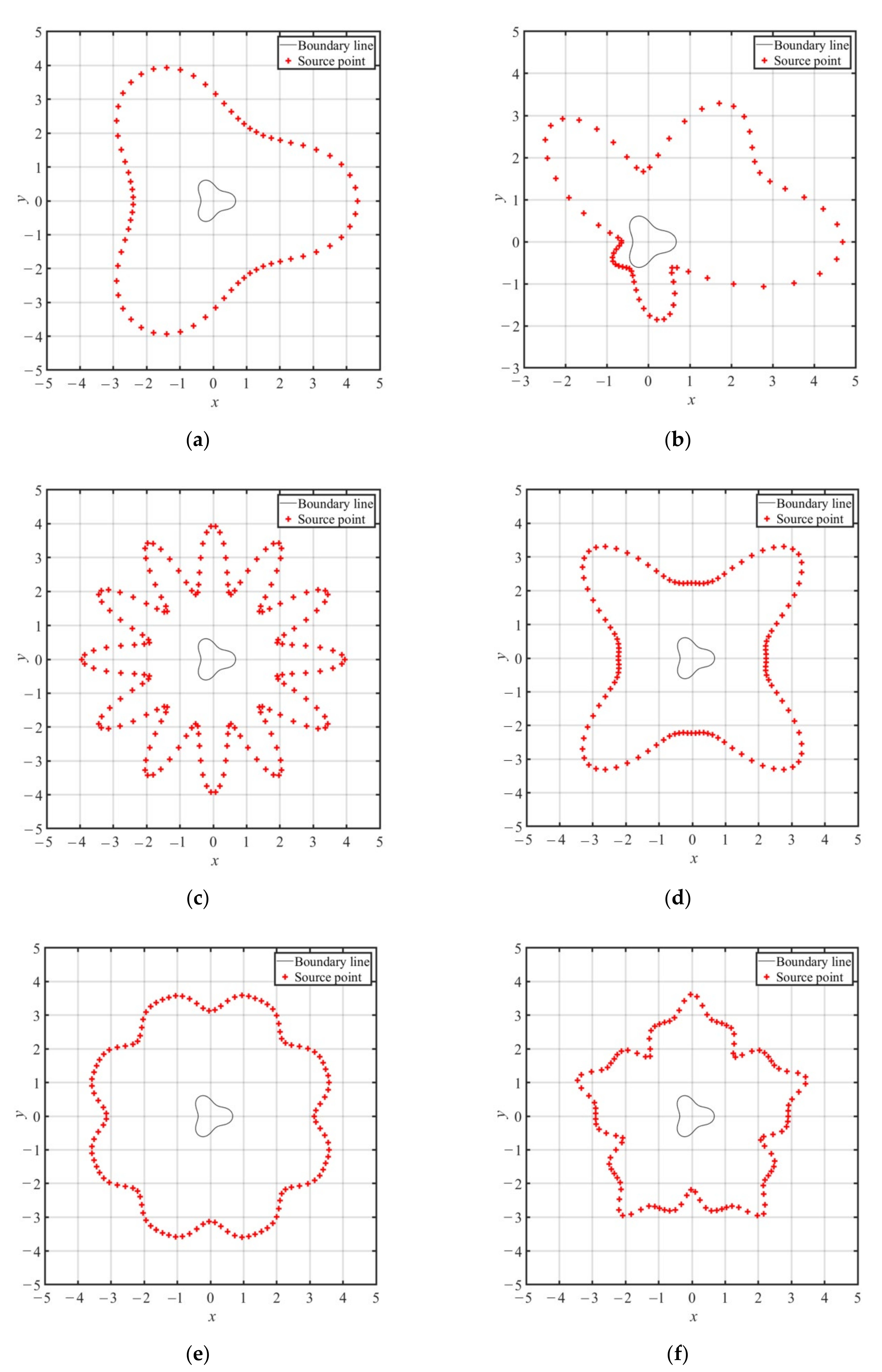
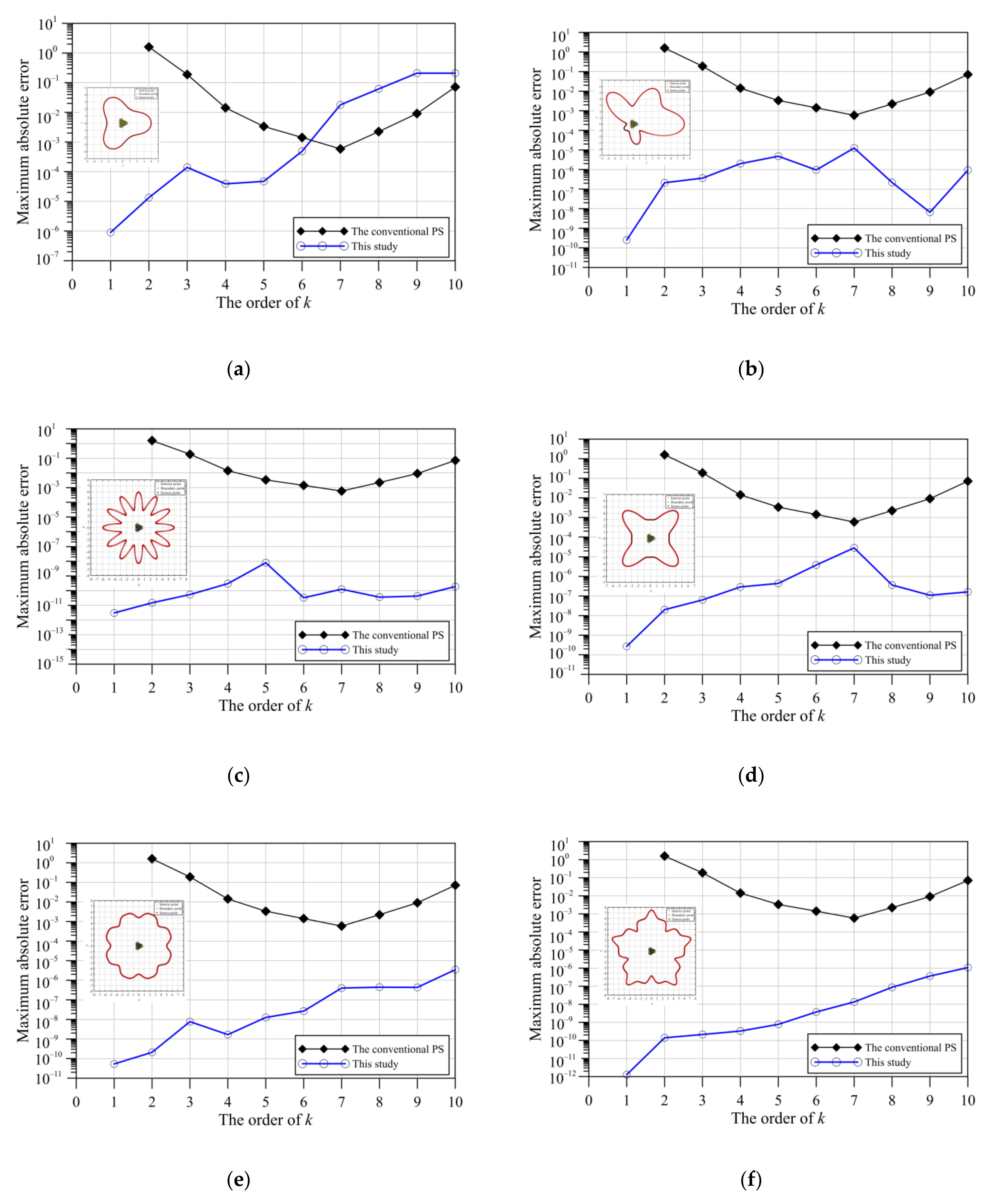
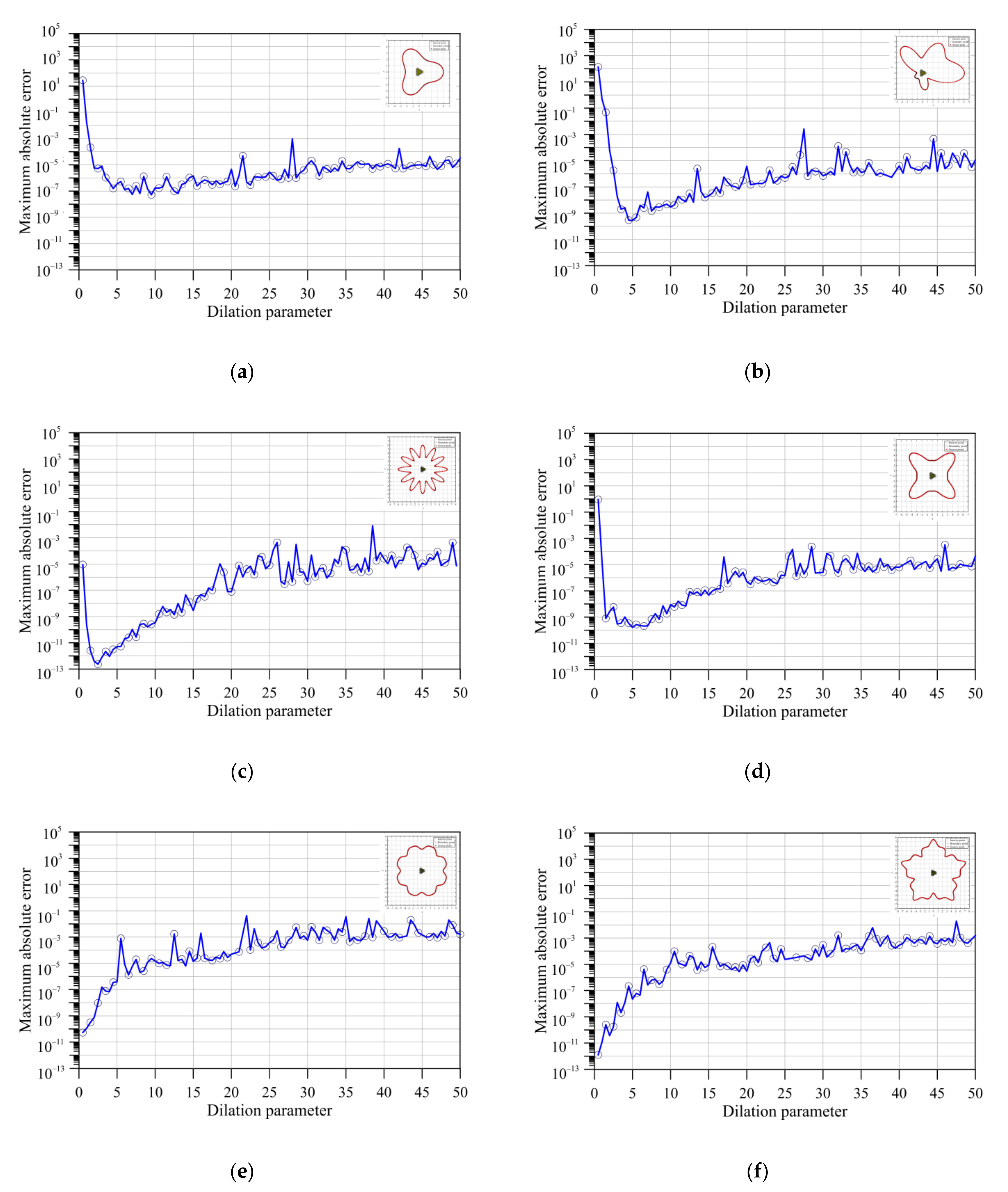
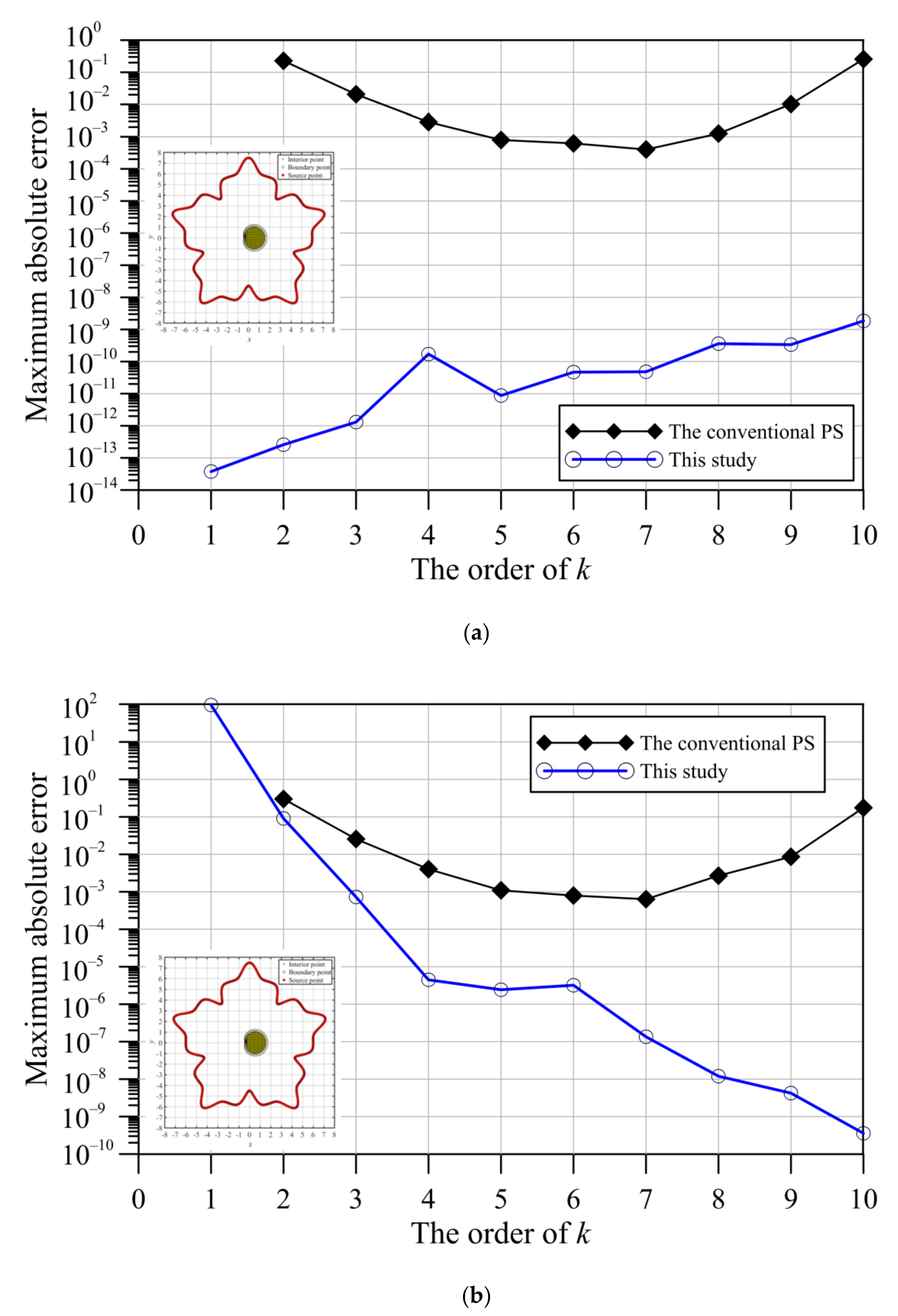
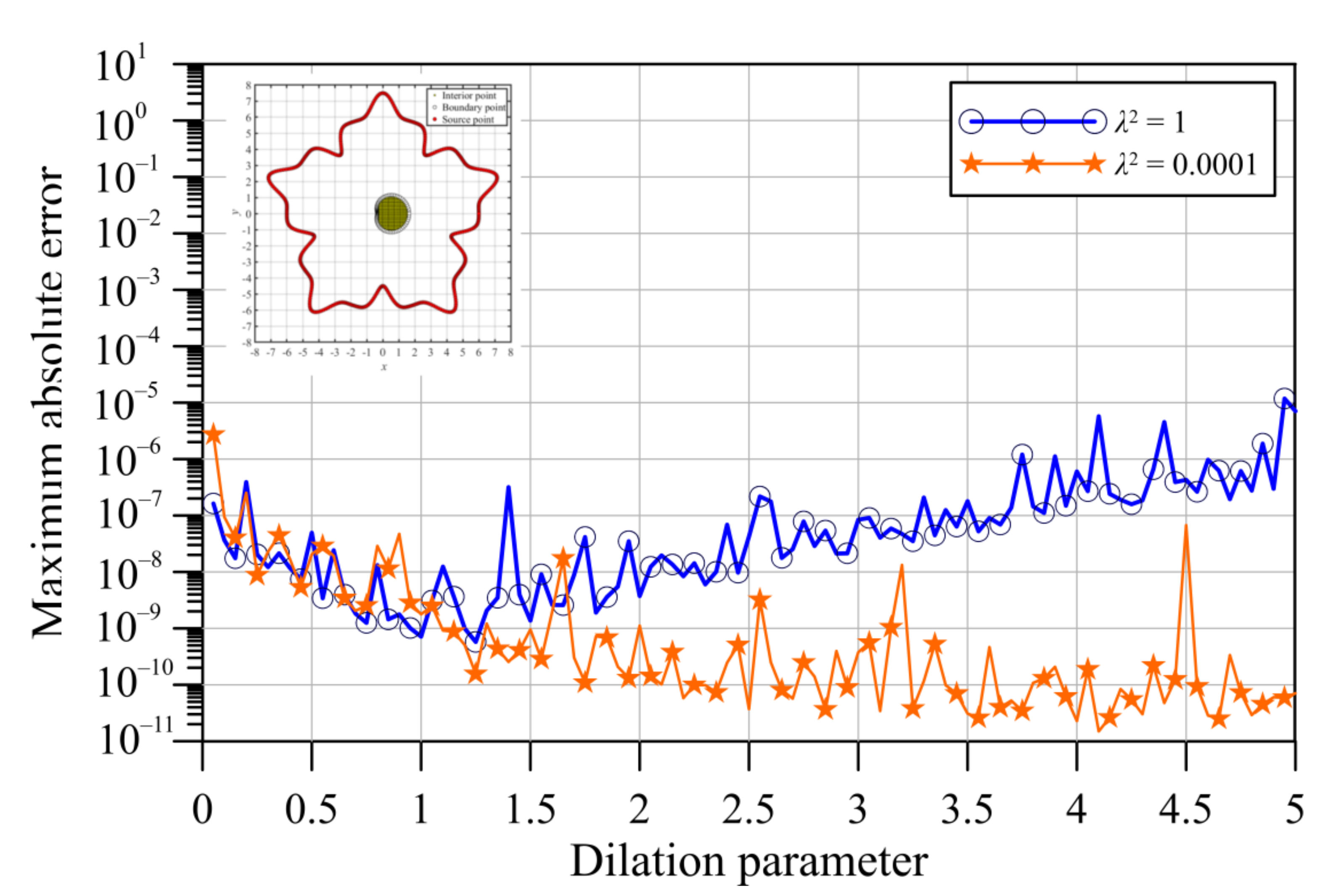
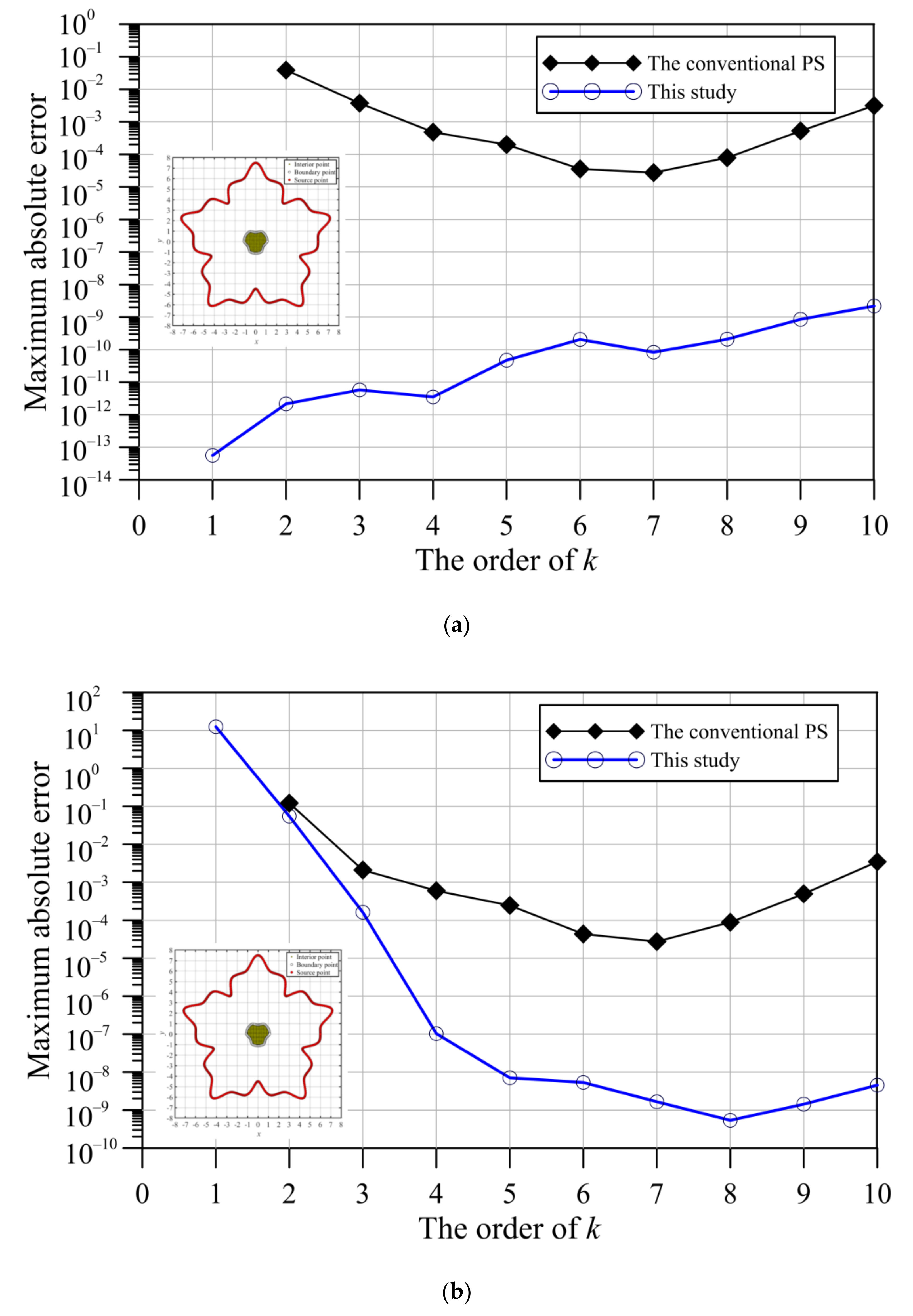
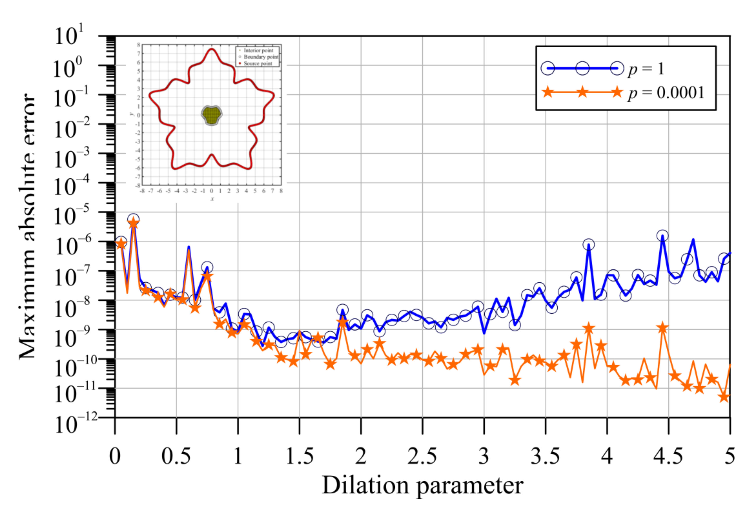
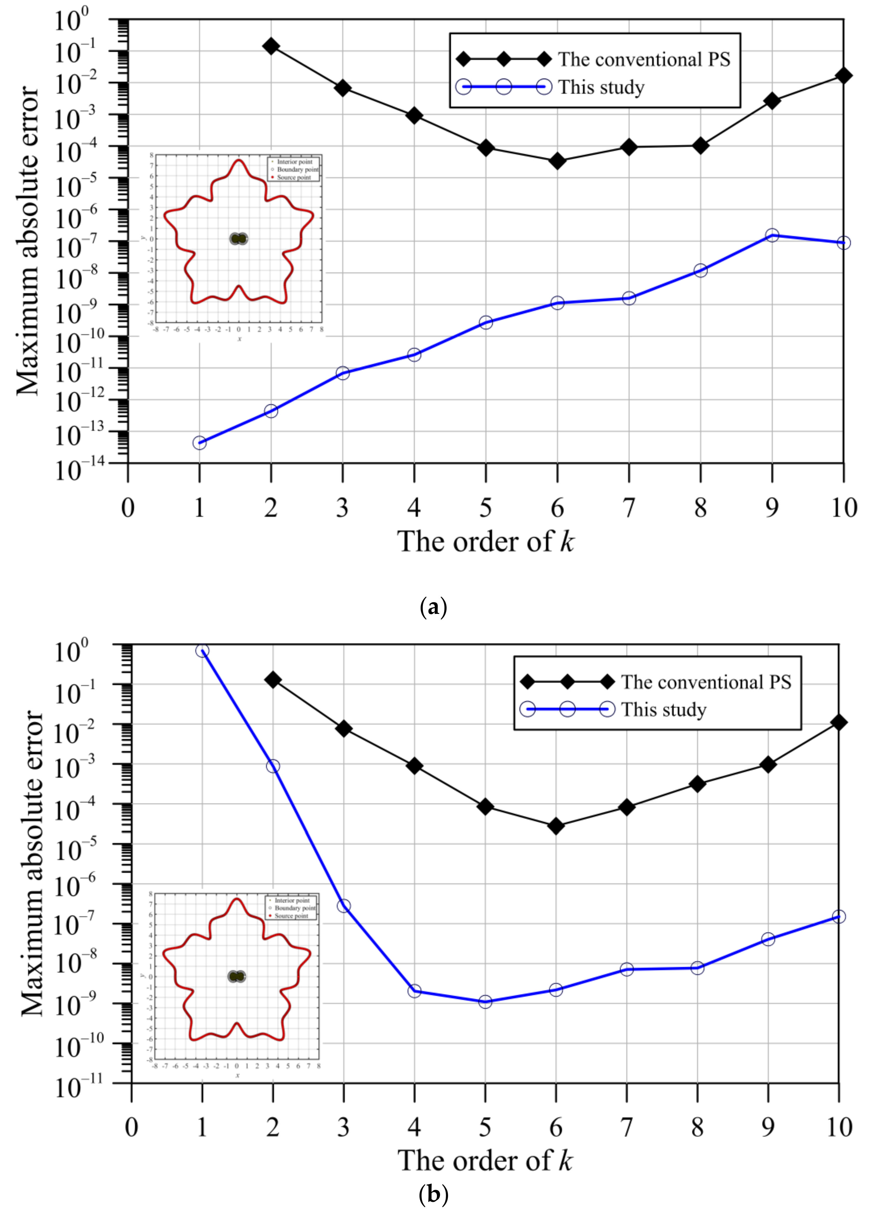
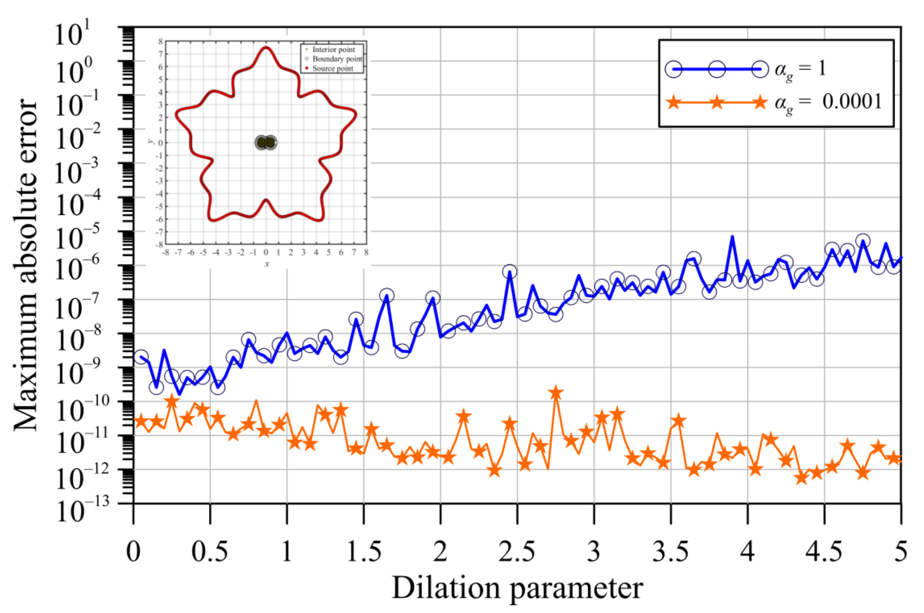
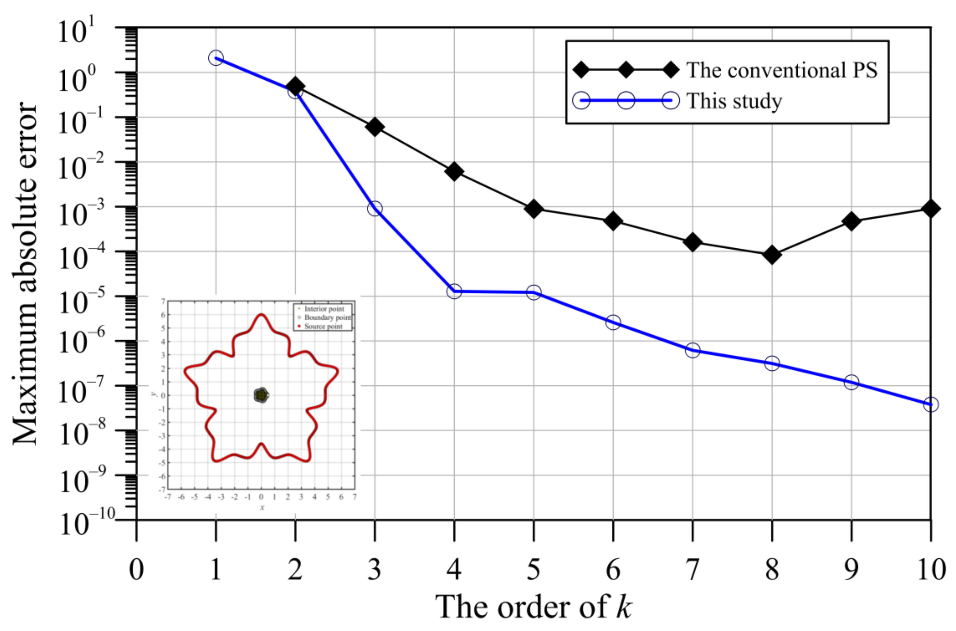
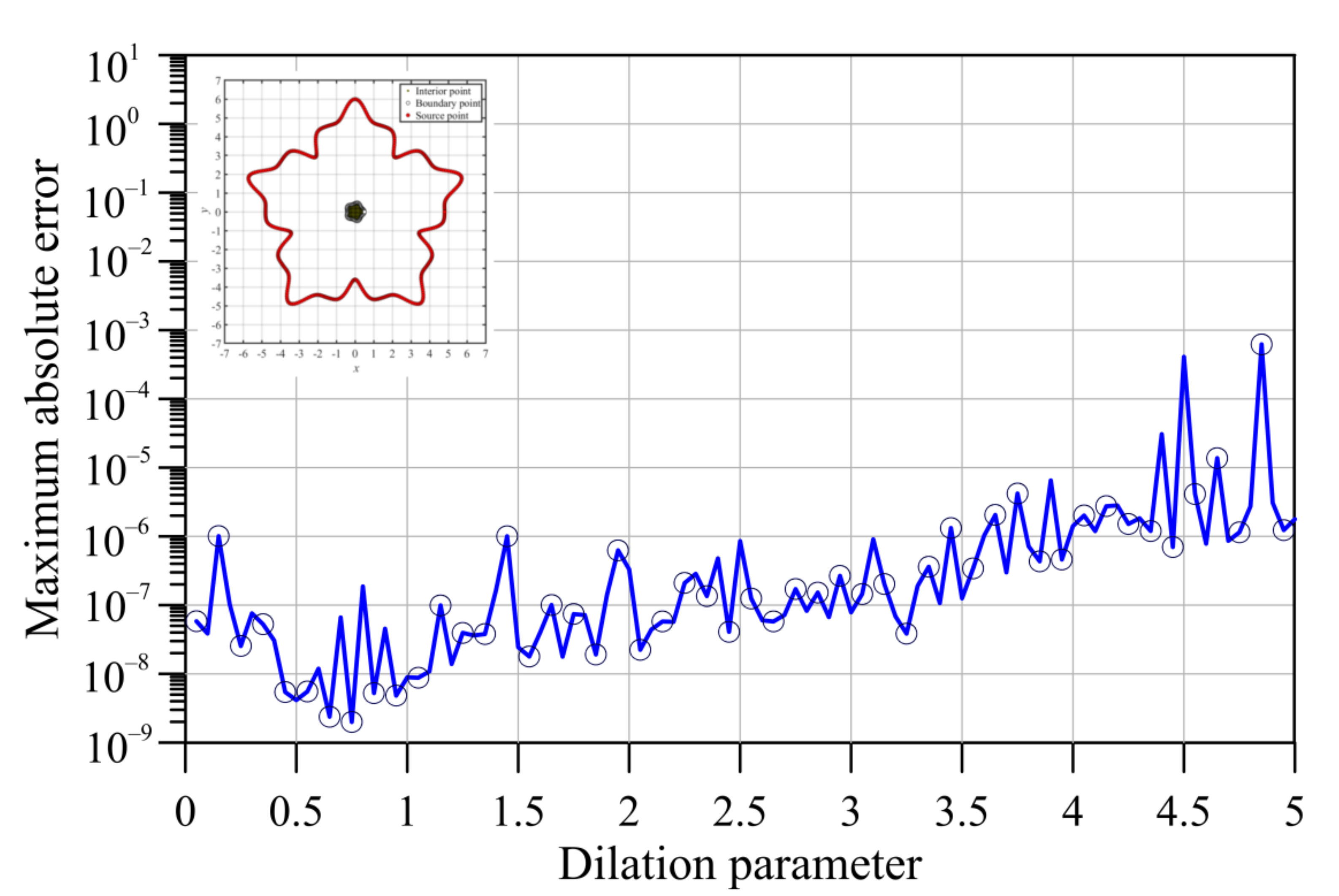
To clarify the possible influences for the positions of the sources on the accuracy, an analysis was conducted to evaluate the accuracy versus the shapes and positions of sources. The results show that the error may grow with the increase of the dilation parameter. However, results from all cases reveal that we may obtain accurate results with the use of an arbitrary value in the range of 1.5 to 5 for the dilation parameter. Nevertheless, the error may increase while the larger dilation parameter is adopted. However, it reveals that we could still obtain better accuracy than original PS even in the worst case. Furthermore, it appears that the accuracy may be less sensitive to the order k from the numerical results. It is found that accurate results with order k in the range of 3 to 10 were acquired.

(3)

The seismic wave propagation problem, groundwater flow problem, unsaturated flow problem, and groundwater contamination problem were investigated to show the robustness and accuracy of the proposed approach. From the results, the proposed infinitely smooth PRBF could provide much more accurate solutions than the conventional PRBF even with the optimal order.

References

1. Liu, C.Y.; Ku, C.Y.; Huang, C.C.; Lin, D.G.; Yeih, W.C. Numerical solutions for groundwater flow in unsaturated layered soil with extreme physical property contrasts. Int. J. Nonlinear Sci. Numer. Simul. 2015, 16, 325–335. [Google Scholar] [CrossRef]
2. Vu, T.D.; Ni, C.F.; Li, W.C.; Truong, M.H.; Hsu, S.M. Predictions of groundwater vulnerability and sustainability by an integrated index-overlay method and physical-based numerical model. J. Hydrol. 2021, 596, 126082. [Google Scholar] [CrossRef]
3. Gu, Y. Meshfree methods and their comparisons. Int. J. Comput. Methods 2005, 2, 477–515. [Google Scholar] [CrossRef]
4. Hon, Y.C.; Chen, W. Boundary knot method for 2D and 3D Helmholtz and convection–diffusion problems under complicated geometry. Int. J. Numer. Methods Eng. 2003, 56, 1931–1948. [Google Scholar] [CrossRef] [Green Version]
5. Ling, L.; Opfer, R.; Schaback, R. Results on meshless collocation techniques. Eng. Anal. Bound. Elem. 2006, 30, 247–253. [Google Scholar] [CrossRef] [Green Version]
6. Xiong, J.; Wen, J.; Liu, Y.-C. Localized boundary knot method for solving two-dimensional Laplace and Bi-Harmonic equations. Mathematics 2020, 8, 1218. [Google Scholar] [CrossRef]
7. Li, P.W. Space–time generalized finite difference nonlinear model for solving unsteady Burgers’ equations. Appl. Math. Lett. 2020, 114, 106896. [Google Scholar] [CrossRef]
8. Chen, W.; Fu, Z.J.; Chen, C.S. Recent Advances in Radial Basis Function Collocation Methods; Springer: Berlin/Heidelberg, Germany, 2014. [Google Scholar]
9. Ma, Z.; Li, X.; Chen, C.S. Ghost point method using RBFs and polynomial basis functions. Appl. Math. Lett. 2021, 111, 106618. [Google Scholar] [CrossRef]
10. Fornberg, B.; Natasha, F. Solving PDEs with radial basis functions. Acta Numer. 2015, 24, 215. [Google Scholar] [CrossRef] [Green Version]
11. Chen, C.S.; Karageorghis, A.; Dou, F. A novel RBF collocation method using fictitious centres. Appl. Math. Lett. 2020, 101, 106069. [Google Scholar] [CrossRef]
12. Hardy, R. Multiquadric equations of topography and other irregular surfaces. J. Geophys. Res. 1971, 76, 1905–1915. [Google Scholar] [CrossRef]
13. Gu, J.; Jung, J.H. Adaptive Gaussian radial basis function methods for initial value problems: Construction and comparison with adaptive MQ RBF methods. J. Comput. Appl. Math. 2020, 381, 113036. [Google Scholar] [CrossRef]
14. Beatson, R.K.; Light, W.A. Fast evaluation of radial basis functions: Methods for two-dimensional polyharmonic splines. IMA J. Numer. Anal. 1997, 17, 343–372. [Google Scholar] [CrossRef]
15. Madych, W.R.; Nelson, S.A. Polyharmonic cardinal splines. J. Approx. Theory 1990, 60, 141–156. [Google Scholar] [CrossRef] [Green Version]
16. Xiang, S.; Bi, Z.Y.; Jiang, S.X.; Jin, Y.X.; Yang, M.S. Thin plate spline radial basis function for the free vibration analysis of laminated composite shells. Compos. Struct. 2011, 93, 611–615. [Google Scholar] [CrossRef]
17. Tsai, C.C.; Cheng, A.D.; Chen, C.S. Particular solutions of splines and monomials for polyharmonic and products of Helmholtz operators. Eng. Anal. Bound. Elem. 2009, 33, 514–521. [Google Scholar] [CrossRef]
18. Sarra, S.A.; Sturgill, D. A random variable shape parameter strategy for radial basis function approximation methods. Eng. Anal. Bound. Elem. 2009, 33, 1239–1245. [Google Scholar] [CrossRef]
19. Biazar, J.; Hosami, M. An interval for the shape parameter in radial basis function approximation. Appl. Math. Comput. 2017, 315, 131–149. [Google Scholar] [CrossRef]
20. Segeth, K. Polyharmonic splines generated by multivariate smooth interpolation. Comput. Math. Appl. 2019, 78, 3067–3076. [Google Scholar] [CrossRef]
21. Fasshauer, G.E. RBF collocation methods as pseudospectral methods. WIT Trans. Model. Simul. 2005, 39, 10. [Google Scholar]
22. Krowiak, A. Radial basis function-based pseudospectral method for static analysis of thin plates. Eng. Anal. Bound. Elem. 2016, 71, 50–58. [Google Scholar] [CrossRef]
23. Fasshauer Gregory, E.; Mccourt Michael, J. Stable evaluation of Gaussian radial basis function interpolants. SIAM J. Sci. Comput. 2012, 34, 737–762. [Google Scholar] [CrossRef]
24. Gholampour, F.; Hesameddini, E.; Taleei, A. A global RBF-QR collocation technique for solving two-dimensional elliptic problems involving arbitrary interface. Eng. Comput. 2020, 1–19. [Google Scholar] [CrossRef]
25. Gonzalez-Rodriguez, P.; Bayona, V.; Moscoso, M.; Kindelan, M. Laurent series based RBF-FD method to avoid ill-conditioning. Eng. Anal. Bound. Elem. 2015, 52, 24–31. [Google Scholar] [CrossRef] [Green Version]
26. Bayona, V.; Flyer, N.; Fornberg, B.; Barnett, G.A. On the role of polynomials in RBF-FD approximations: II. Numerical solution of elliptic PDEs. J. Comput. Phys. 2017, 332, 257–273. [Google Scholar] [CrossRef] [Green Version]
27. Shcherbakov, V.; Larsson, E. Radial basis function partition of unity methods for pricing vanilla basket options. Comput. Math. Appl. 2016, 71, 185–200. [Google Scholar] [CrossRef]
28. Cavoretto, R.; De Marchi, S.; De Rossi, A.; Perracchione, E.; Santin, G. Partition of unity interpolation using stable kernel-based techniques. Appl. Numer. Math. 2017, 116, 95–107. [Google Scholar] [CrossRef] [Green Version]
29. Rashidinia, J.; Fasshauer, G.E.; Khasi, M. A stable method for the evaluation of Gaussian radial basis function solutions of interpolation and collocation problems. Comput. Math. Appl. 2016, 72, 178–193. [Google Scholar] [CrossRef]
30. Wright, G.B.; Fornberg, B. Stable computations with flat radial basis functions using vector-valued rational approximations. J. Comput. Phys. 2017, 331, 137–156. [Google Scholar] [CrossRef] [Green Version]
31. De Marchi, S.; Martínez, A.; Perracchione, E. Fast and stable rational RBF-based partition of unity interpolation. J. Comput. Appl. Math. 2019, 349, 331–343. [Google Scholar] [CrossRef]
32. Bawazeer, S.A.; Baakeem, S.S.; Mohamad, A.A. New approach for radial basis function based on partition of unity of Taylor series expansion with respect to shape parameter. Algorithms 2021, 14, 1. [Google Scholar] [CrossRef]
33. Ku, C.Y.; Liu, C.Y.; Xiao, J.E.; Hsu, S.M. Multiquadrics without the shape parameter for solving partial differential equations. Symmetry 2020, 12, 1813. [Google Scholar] [CrossRef]
34. Ku, C.Y.; Liu, C.Y.; Xiao, J.E.; Hsu, S.M.; Yeih, W. A collocation method with space–time radial polynomials for inverse heat conduction problems. Eng. Anal. Bound. Elem. 2021, 122, 117–131. [Google Scholar] [CrossRef]
35. Cao, L.; Qin, Q.H.; Zhao, N. An RBF–MFS model for analysing thermal behaviour of skin tissues. Int. J. Heat Mass Transf. 2010, 53, 1298–1307. [Google Scholar] [CrossRef]
36. Mai-Duy, N.; Tran-Cong, T. Indirect RBFN method with thin plate splines for numerical solution of differential equations. CMES Comp. Model. Eng. Sci. 2003, 4, 85–102. [Google Scholar]
37. Li, J.; Zhai, S.; Weng, Z.; Feng, X. H-adaptive RBF-FD method for the high-dimensional convection-diffusion equation. Int. Commun. Heat Mass Transf. 2017, 89, 139–146. [Google Scholar] [CrossRef]
Figure 1. Location of the collocation points: (a) the conventional PRBF; (b) this study.
Mathematics 09 01535 g001
Figure 2. The fictitious sources at different positions: (a) Case I; (b) Case II; (c) Case III; (d) Case IV; (e) Case V; (f) Case VI.
Mathematics 09 01535 g002
Figure 3. The computed MAE values for the original PRBF and the proposed PRBF with fictitious sources: (a) Case I; (b) Case II; (c) Case III; (d) Case IV; (e) Case V; (f) Case VI.
Mathematics 09 01535 g003
Figure 4. The computed MAE versus the dilation parameter ( k = 1 ) (a) Case I; (b) Case II; (c) Case III; (d) Case IV; (e) Case V; (f) Case VI.
Mathematics 09 01535 g004
Figure 5. The conventional radial basis function collocation method (RBFCM) collocation scheme.
Mathematics 09 01535 g005
Figure 6. The fictitious sources.
Mathematics 09 01535 g006
Figure 7. The computed MAE values of the original PRBF and the proposed method: (a) λ 2 = 0.0001 ; (b) λ 2 = 1 .
Mathematics 09 01535 g007
Figure 8. Maximum absolute error versus the dilation parameter ( k = 6 ) .
Mathematics 09 01535 g008
Figure 9. The conventional RBFCM collocation scheme.
Mathematics 09 01535 g009
Figure 10. The fictitious sources.
Mathematics 09 01535 g010
Figure 11. The computed MAE values of the original PRBF and the proposed method: (a) p = 0.0001; (b) p = 1.
Mathematics 09 01535 g011
Figure 12. Maximum absolute error versus the dilation parameter ( k = 7 ) .
Mathematics 09 01535 g012
Figure 13. The conventional RBFCM collocation scheme.
Mathematics 09 01535 g013
Figure 14. The fictitious sources.
Mathematics 09 01535 g014
Figure 15. The computed MAE values of the original PRBF and the proposed method: (a) α g = 0.0001 ; (b) α g = 1 .
Mathematics 09 01535 g015
Figure 16. Maximum absolute error versus the dilation parameter ( k = 4 ) .
Mathematics 09 01535 g016
Figure 17. The conventional RBFCM collocation scheme.
Mathematics 09 01535 g017
Figure 18. The fictitious sources.
Mathematics 09 01535 g018
Figure 19. The computed MAE values of the original PS and the proposed method.
Mathematics 09 01535 g019
Figure 20. Maximum absolute error versus the dilation parameter ( k = 10 ) .
Mathematics 09 01535 g020