Dead-Time Compensation for the First-Order Dead-Time Processes: Towards a Broader Overview

Abstract

The article reviews the results of a number of recent papers dealing with the revision of the simplest approaches to the control of first-order time-delayed systems. The concise introductory review is extended by an analysis of two discrete-time approaches to dead-time compensation control of stable, integrating, and unstable first-order dead-time processes including simple diagnostics of the model used and focusing on the possibility of simplified but reliable plant modelling. The first approach, based on the first historically known dead-time compensator (DTC) with possible dead-beat performance, is based on the reconstruction of the actual process variables and the compensation of input disturbances by an extended state observer (ESO). Such solutions play an important role both in a disturbance observer (DOB) based control and in an active disturbance rejection control (ADRC). The second approach considered comes from the Smith predictor with two degrees of freedom, which combines feedforward control with output disturbance reconstruction and compensation by the parallel plant model. It is shown that these two approaches offer advantageous properties in the case of actuator limitations, in contrast to the commonly used PID controllers. However, when applied to integrating and unstable first-order systems, the unconstrained and possibly unobservable output disturbance signal of the second solution must be eliminated from the control loop, due to the hidden structural instability of the Smith predictor-like solutions. The modified solutions, usually referred to as filtered Smith predictor (FSP), then no longer provide a disturbance signal and thus no longer fully fit into the concept of Industry 4.0, which is focused on further optimization, predictive maintenance in dynamic systems, diagnosis, fault detection and fault identification of dynamic processes and forms the basis for the digitalization of smart production. Nevertheless, the detailed analysis of the elimination of the unstable disturbance response mode is also worth mentioning in terms of other possible solutions. The application of both approaches to the control of a thermal process shows almost equivalent quality, but with different dependencies on the tuning parameters used. It is confirmed that a more detailed identification of the controlled process and the resulting higher complexity of the control algorithms does not necessarily lead to an increase in the resulting quality of the transients, which underlines the importance of the simplified plant modelling for practice.

1. Introduction

Time delays due to the terminal velocity of information transmission and processing, the computational speed of computers, or the terminal velocity of mass and energy transport are among the fundamental aspects of the control of dynamical systems. We encounter them in innumerable variations across the spectrum of scientific and engineering disciplines [1,2,3,4,5,6,7].

First-order time-delayed (FOTD) systems are the most commonly used process models in control design [8]. In addition to their use in classical tuning methods, they are also successfully used in model-based control. Two basic types of model-based controllers that incorporate transport delays are dead-time compensators (DTCs) and proportional-integral-derivative (PID) controllers. Skogestad [9] has shown that classical PID controllers can result from a delayed-model approach when the delay is replaced by the first terms of Padé or Taylor series approximations. Such simplifications [10] were common in the analog controller era, when implementing dead time was a major challenge. Today, the implementation of time delays in digital controllers is trivial. In this context, the time-shift operation in dead time modelling and simulation is the basic functionality. In terms of dead-time approximations, it is therefore surprising that there were still doubts whether DTCs (i.e., the “more accurate” solutions) are indeed more robust than the “less accurate” approximate solutions based on PID controllers [9,11]. Should the approximate solutions really guarantee higher robustness than the DTCs based on exact delays? Is this also true for the higher-order PIDs (HO) discussed in [10,12] with the aim to obtain more degrees of freedom for designers to meet a predefined set of performance criteria, especially to increase performance and robustness for noisy and uncertain systems? These contributions lead to the first question, whether the solutions based on DTCs and PIDs are correctly interpreted and understood, and whether they can be considered equivalent. However, there are several other unanswered or unresolved questions related to the design of DTCs that are uncovered in this paper.

The best known DTC, originally designed as a Smith predictor (SP) [13], can only be applied to stable FOTD systems. Therefore, its extension to integrating and unstable systems is still the goal of current research. However, in addition to the further development of FSPs [14,15,16], DTCs for unstable and integrating systems can also be designed as stabilized solutions that still provide the disturbance signal, which is important for many applications. The stabilizing controller designed correctly for an unstable plant can first yield a stable circuit with known dominant dynamics, for which we then propose a disturbance observer in the usual way [17]. Alternatively, we may design the feedforward control and disturbance reconstruction and compensation separately, and use reference models to incorporate a stabilizing controller into the overall structure without nominally affecting the operation of the basic (lower-level) loops [18].

The first aim of this paper is to extend these two two-step approaches to design of DTCs with explicitly reconstructed disturbance signal to integrating and unstable processes by showing the third (direct) possibility when the stabilizing controller and the disturbance reconstruction in the state-space are designed using the extended state observer (ESO) [19,20]. This original solution providing dead-beat performance preceded the development in both the ADRC and Disturbance Observer-based controller design domains. In this paper, it is complemented by a simple filtering technique that allows for the consideration of noise and uncertainty.

The second aim is to analyse in details all significant features of the discrete-time Smith predictor inspired solutions applied possibly also to unstable and integral plants [14,16,17,18,21,22]. This, however, requires elimination of the unstable plant mode from the disturbance response and also elimination of the disturbance signal from the controller structure. The detailed analysis of these eliminations is also worth mentioning in terms of other possible solutions.

Moreover, as Ziegler and Nichols [23] pointed out in their pioneering work, which was later followed by numerous other contributions in the area of Active Disturbance Rejection Control (ADRC, [24,25]) or Model Free Control (MFC, [26]), but they have already been noticed by authors from the field of PID control [12,27], the simple integrating models can also be attractive for the design of simplified DTCs on the simplest stable processes [18].

The rest of the paper is structured as follows: Section 2 deals with the modelling problems, the approximation of model uncertainties by input and output disturbances, the design of stabilizing P controllers, and the state and disturbance reconstruction in time-delayed systems, using the state-space and polynomial approaches. The proposed controllers are illustrated by Example 1. Section 3 continues this work with a special focus on Smith Predictor-inspired approaches. Example 2 provides a comparison of the two types of the DTCs considered and Example 3 gives analyses of the control constraints impact. The application of both types of DTCs is also illustrated in Section 4, with an example of the control of a thermal process. Although the thermal process represents a typical stable system, the use of solutions based on integrating models provides an interesting opportunity to simplify the whole process modelling and the corresponding DTC designs. The main results obtained are discussed in Section 5 and summarized in the conclusions.

2. Modelling and Controller Design for the Simplest Time-Delayed Processes

In order to generalize and modify SP (and other DTCs) for all types of processes (e.g., integrating and unstable), we first need to interpret it in a more concise way. For several decades now, SP modifications for integrating and unstable systems have not been explained sufficiently consistently (as, e.g., discussed in [18]). This can be one of the sources of distrust of DTCs expressed in [9,11], or in surveys on the importance of control structures for introductory control courses [28]. In terms of design interpretation, there are several options.

Dead-time elimination. One possible interpretation of SP is that its advantage is to remove the transport delay from the characteristic polynomial of the closed-loop [29,30]. However, such an interpretation gives only limited information about the closed-loop response. Indeed, the disturbance response with all model imperfections is still affected by time delays in the loop, which must be taken into account when choosing the controller structure and tuning.

Output reconstruction/prediction. The second possible interpretation of SP is the reconstruction of the actual (not-delayed) plant output of the system from the series of delayed measurements of the input and output signals of the plant [29,31]. The same results can be derived by generating the control signal from a predicted process output value, which can be calculated by applying the control signal samples accumulated in the system input delay. Inspired by some older works by de Paor [32,33,34], such an interpretation of time delay compensation has been used much earlier [19,20,35,36] in combination with stabilizing P or PD controllers with two degrees of freedom (2-DoF) in the setpoint tracking channel and with input disturbance reconstruction and compensation. The preferred use of input (load) disturbance reconstruction resulted from the unobservability of the output disturbances in combination with integrating models.

Dynamical setpoint feedforward and output disturbance rejection. The third interpretation considers SP as a feedforward control realized by a primary loop complemented by a secondary output disturbance rejection loop acting on the reference setpoint signal.

The last two interpretations are further clarified by designing DTCs in the state space and in generalizing the SP. However, the reliable implementation of DTCs requires the solution of numerous other problems. In this regard, it is necessary to explain:

• The principles of setpoint and disturbance feedforward control and the conditions for their use;
• The effects of external and internal, input and output disturbances and their role in compensating plant uncertainties;
• The reconstruction of output and input disturbances by the parallel and inverse plant models and how such feedback transforms the controlled plant;
• Why a setpoint feedforward through the primary loop is used and the role of control constraints and unstable plant dynamics in such control;
• Stabilization based on zero setpoint tracking error and zero total input disturbance;
• Why to apply integrating models even for non-integrating plants;
• How to introduce experimentally verifiable robustness measures suitable for all stable, integrating and unstable plants in the time domain;
• How to attenuate the measurement noise by an appropriate filter design.

2.1. Two Types of Linear Models for First-Order Dominant Plant Dynamics

When modelling the first-order time-delayed plant with output $y\left(t\right)$ and input $u\left(t\right)$, one might expect optimal control behaviour if the model parameters $K_{sm}$, $a_m$ and $T_{dm}$ in

$$\begin{array}{c}{S}_{dm}\left(s\right)={\displaystyle \frac{Y\left(s\right)}{U\left(s\right)}}=S_m\left(s\right)e^{-T_{dm}s};S_m\left(s\right)={\displaystyle \frac{K_{sm}}{s+a_m}}\hfill \end{array}$$

(1)

approach the parameters $K_s,a$ and $T_d$ of a “nominal real” plant $S\left(s\right)$

$$\begin{array}{c}S\left(s\right)={\displaystyle \frac{Y\left(s\right)}{U\left(s\right)}}=S_0\left(s\right)e^{-T_{d}s};S_0\left(s\right)={\displaystyle \frac{K_s}{s+a}}\hfill \end{array}$$

(2)

Remark 1.

However, the assumption that the “nominal” model is well-defined has no solid basis in practice. The majority of plants have “no real parameters” and the model parameters are just numbers ( knobs ) used to approximate a more or less complex real plant behaviour. The notion of “nominal” plant dynamics may be useful in the simulation environment, but this does not mean that the nominal model can be obtained in practice and then used as a standard for evaluating experiments.

A commonly used simplification is to neglect the process time constant by simply considering $a_m=0$ (instead of $a_m=a$). In this way, one can deliberately work with an even simpler integrator-plus-dead-time (IPDT) model, even when dealing with clearly stable plants. Such an approach, motivated by simplified path identification or simplified controller design (or both), is routinely used. As an example, one of the most commonly cited methods for plant identification is based on a tangent line drawn through an inflection point of the plant step response [23], which may well be interpreted by the IPDT model [37]. Other well-known examples are Model Free Control (MFC) [38] and the Active Disturbance Rejection Control (ADRC) with an Extended State Observer (ESO) [5,24,39,40]. A similar conclusion was reached in the design of PI and PID control by [27,41]. However, in DTCs based on Internal Model Control (IMC), which includes the SP-inspired structures, the integrating process model leads to significant problems.

Another issue in DTC-related works that deserves a more detailed analysis is the advantage of discrete-time realization. Namely, the advantage is a simpler and more accurate modelling of transport delays in digital circuits. On the other hand, since the sampling period can be neglected, the continuous-time nomenclature is mostly used today because of the simpler description. To the best of our knowledge, there are no recent works dealing with the analog dead-time implementation in controller design, which is performed in the continuous-time domain. Therefore, we will not address continuous-time controller design for integrating systems in this paper with respect to digital implementation of standard industrial controllers [31,42].

For discrete-time control with a sampling period $T_s$ satisfying $T_{dm}=k_m{T}_s,k_m\in {\mathbf{Z}}^{+}$ and z representing the shift operator, the model of the FOTD plant (1), changes in the discrete-time domain to

$$\begin{array}{c}{S}_{dm}\left(z\right)=S_m\left(z\right)z^{-k_m};S_m\left(z\right)={\displaystyle \frac{K_m}{z-D_m}};\mathrm{where}\mathrm{for}\hfill \\ a_m=0,K_m=K_{sm}{T}_s;D_m=1;\hfill \\ a_m\ne 0,K_m={\displaystyle \frac{K_{sm}(1-D_m)}{a_m}};D_m=e^{-a_m{T}_s}.\hfill \end{array}$$

(3)

Let us define the discrete-time model of the real plant for the nominal case:

$$S\left(z\right)=S_0\left(z\right)z^{-k};S_0\left(z\right)=K/(z-D).$$

(4)

2.2. Model Uncertainties and Setpoint Feedforward

From a control design point of view, it is important to mention that closed-loop performance is significantly affected by external disturbances and model imperfections resulting from uncertainties caused by modelling, identification, time-varying nature of systems, nonlinearities, etc. [41,43]. These uncertainties can be considered as internal disturbances. It should be emphasized that the acting disturbances and uncertainties are the main reason for using feedback in automatic control and both have a significant impact on the controller design.

Starting with the simplest case, where a reference setpoint w is filtered by the first-order low-pass filter $Q_w\left(s\right)$ with a gain of one and a time constant $T_c>0$ [18], the simple feedforward block $C_w\left(s\right)$ used for an open-loop generation of the feedforward control signal $u_{wf}$, can be designed as

$$C_w\left(s\right)={\displaystyle \frac{U_{wf}\left(s\right)}{W\left(s\right)}}={\displaystyle \frac{Q_w\left(s\right)}{S_m\left(s\right)}};Q_w\left(s\right)={\displaystyle \frac{1}{1+T_{c}s}}.$$

(5)

Similarly, in the discrete-time domain, the filtered feedforward could be calculated as

$$C_w\left(z\right)={\displaystyle \frac{U_{wf}\left(z\right)}{W\left(z\right)}}={\displaystyle \frac{Q_w\left(z\right)}{S_m\left(z\right)}};Q_w\left(z\right)={\displaystyle \frac{1-D_c}{z-D_c}};D_c=e^{-T_s/T_c}.$$

(6)

The low-pass filters $Q_w\left(s\right)$ and $Q_w\left(z\right)$ make the feedforward $C_w\left(s\right)$ and $C_w\left(z\right)$ proper and determine the speed of the output response.

For example, consider the uncertainty of the plant model expressed as $a_m=a+\Delta a$, or $D_m=D+\Delta D$. For simplicity, assume that the plant gain is perfectly modelled ($K_{sm}=K_s$, or $K_m=K$). Then, the outputs of the continuous-time and discrete-time feedforward control systems are

$$\begin{array}{c}Y\left(s\right)={\displaystyle \frac{s+a+\Delta a}{s+a}}{Q}_w\left(s\right)W\left(s\right)=(1+{\displaystyle \frac{\Delta a}{s+a}})Q_w\left(s\right)W\left(s\right)\hfill \\ Y\left(z\right)={\displaystyle \frac{z-D+\Delta D}{z-D}}{Q}_w\left(z\right)W\left(z\right)=(1+{\displaystyle \frac{\Delta D}{z-D}})Q_w\left(z\right)W\left(z\right).\hfill \end{array}$$

(7)

It turns out that the model uncertainty corresponds to an “internal” disturbance $\Delta d_i=\Delta a/K_s$, or $\Delta d_i=\Delta D/K$ acting at the input of the continuous-time $S\left(s\right)$ (Equation (2)), or the discrete-time $S\left(z\right)$ (Equation (4)) plant. Although the transients can be made faster by using smaller values of $T_c\to 0$ (or $D_c\to 0$) can be accelerated, for the control of stable systems ($a>0$, $D\in (0,1)$), the fading of the uncertainty perturbations depends on the time constant $T=1/a$. In the case of unstable systems ($a<0$, or $D>1$), “internal” disturbances already lead to an unrestrained increase in the system output and make such a disturbance controller unusable. Since such “exponential” outputs can be interpreted as results of equivalent unimpeded output disturbances $d_o$, in practice, the calculation of output disturbance signals should be avoided in unstable systems, since they can lead to an overflow of the computer’s registers. (Not always, as signal Y is also often limited in practice).

For $K_{sm}\ne K_s$, or $K_m\ne K$, permanent steady-state errors occur, which can again degrade feedforward control even in stable systems. In such situations, as well as when compensating for output disturbances of stable systems, corrective feedback is sufficient to achieve the desired output. However, for the control of unstable systems, stabilizing feedback with elimination of possible input disturbances must be used. In both cases, we must avoid using unbounded output disturbances.

Therefore, considering these factors, we have proceeded with the reconstruction and compensation of input disturbances in the development of integrating controllers based on the reconstruction and compensation of disturbances in the state space, as well as considering the unobservability of output disturbances for integrating models [19,20,35,36].

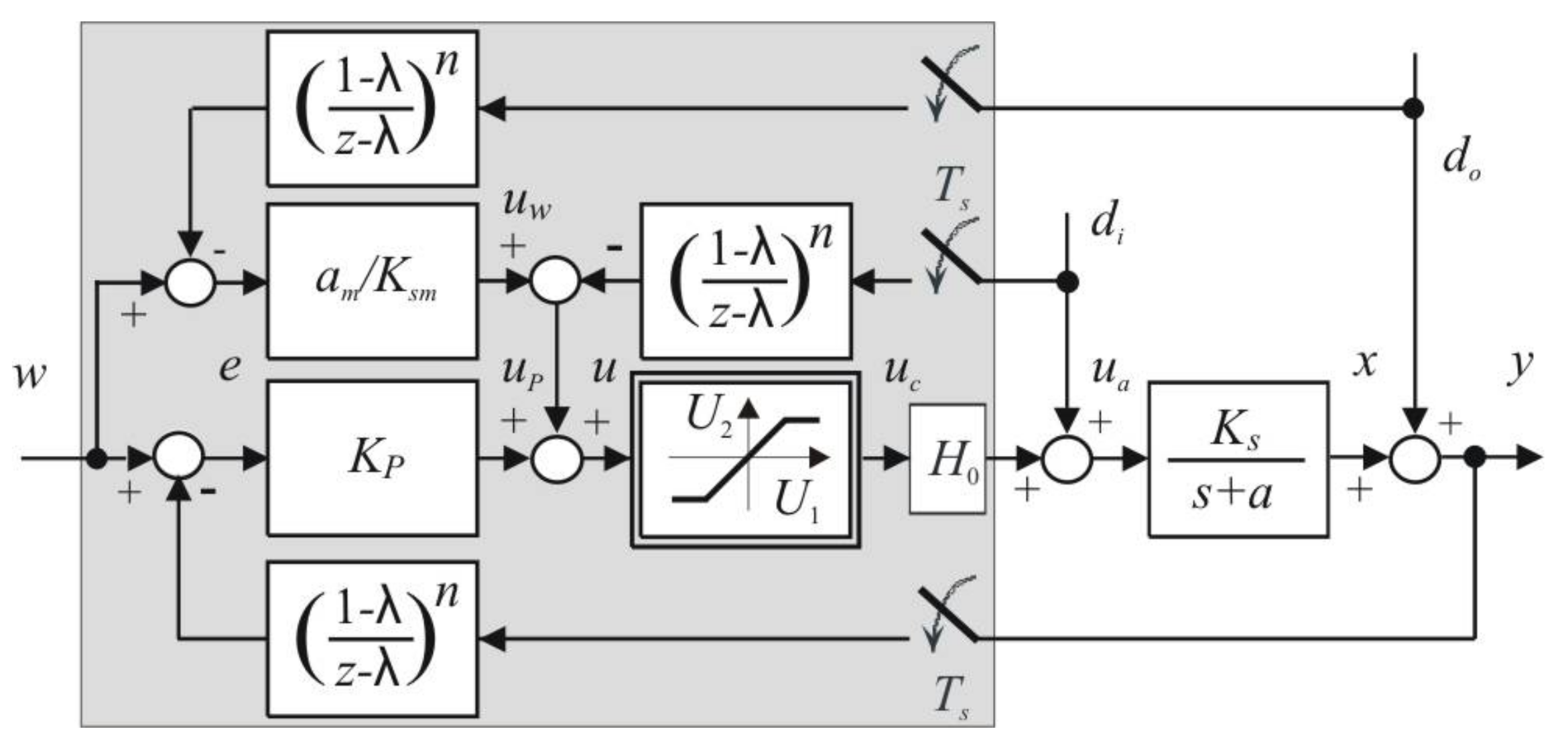
2.3. 2-DoF P Control with Disturbance Feedforward

Let us consider a nominal case with a delay-free plant, $D_m=D$, $a_m/K_{sm}=a/K_s$ and no filtration applied ($n=0$ in Figure 1). For piecewise constant inputs (setpoint w and disturbances $d_i$, $d_o$) and the control error introduced at time instants $t=N{T}_s$ as

$$e\left(N\right)=w\left(N\right)-y\left(N\right),$$

(8)

the plant output difference equation derived for linear control ($u_c=u$) is

$$x(N+1)=K[u\left(N\right)+d_i\left(N\right)]+Dx\left(N\right);y\left(N\right)=x\left(N\right)+d_o\left(N\right).$$

(9)

The monotonic control error decrease requirement can be expressed as

$$e(N+1)=D_{c}e\left(N\right);0\le D_c<1;D_c=e^{-T_s/T_c};T_c>0,$$

(10)

with $D_c=e^{-T_s/T_c}$ denoting the quotient (the closed loop pole) corresponding to the closed loop time constant $T_c>0$. From the expression of the closed loop control error (10) and from Equations (8) and (9), the control signal u may be calculated by means of a two-degree of freedom (2-DoF) P controller:

$$\begin{array}{c}u\left(N\right)=K_{P}e\left(N\right)+\left(w\left(N\right)-d_o\left(N\right)\right)(1+a_m/K_{sm})-d_i\left(N\right);\hfill \\ K_P=(D-D_c)/K;D_c=e^{-\frac{T_s}{T_c}}.\hfill \end{array}$$

(11)

Nominally, for the perfect model gain ($K_m=K$) and no filtration applied ($n=0$), such a controller guarantees setpoint step responses with the output $Y\left(z\right)$ specified by $F_{wy}\left(z\right)$ and the corresponding control signal dynamics $F_{wu}\left(z\right)$

$$\begin{array}{c}{F}_{wy}\left(z\right)={\left[{\displaystyle \frac{Y\left(z\right)}{W\left(z\right)}}\right]}_{d_i=d_o=0}={\displaystyle \frac{1-D_c}{z-D_c}}=Q_w\left(z\right);\hfill \\ F_{wu}\left(z\right)={\left[{\displaystyle \frac{U\left(z\right)}{W\left(z\right)}}\right]}_{d_i=d_o=0}={\displaystyle \frac{1-D_c}{z-D_c}}{\displaystyle \frac{z-D}{K}}={\displaystyle \frac{Q_w}{S_0\left(z\right)}}.\hfill \end{array}$$

(12)

The transfer function $F_{wu}\left(z\right)$ including the plant inverse $S_0^{-1}\left(z\right)$ indicates that such a controller-plant combination may also be useful to generate the filtered setpoint feedforward $W_f=Q_{w}W$. However, it should be mentioned that, since $S_0\left(z\right)$ is not known, the model $S_m\left(z\right)$, should be used instead in the plant model inversion, as given in Equations (5) and (6).

When $D_c\to 0$ (with $T_c/T_s\to 0$) the design offers easily detectable dead-beat performance, celebrated in the early years of digital control as its exceptional achievement. However, as $T_c$ increases, the gain $K_P$ decreases, which also decreases the effect of the measurement noise. Since such noise appears in output and disturbances measurement, the quasi-continuous control with $T_c>>T_s$ may be preferred in the majority of industrial applications. Note that the dead-beat control can still be applied as well, e.g., when evaluating circuit imperfections. It will only need to be used with relatively long sampling times. Nevertheless, in practice, it may be required to introduce an additional filtration for attenuation of the measurement noise.

2.4. Filtered P Controller Design

For an increased noise attenuation in both, the disturbance compensation and the output measurement channels, the additional filters

$$F\left(z\right)={\displaystyle \frac{{(1-\lambda )}^n}{{(z-\lambda )}^n}}$$

(13)

may be used (Figure 1) by selecting $n>1$. As, e.g., mentioned in [44], “more roll-off may contribute to robustness, but excessive roll-off results in peaking of the sensitivity and complementary sensitivity functions”. Since the additional roll-off is only effective when the feedback controller includes the same amount of roll-off, the filters will be introduced simultaneously into both, the output stabilization and the disturbance compensation channels. Their delays characterized by the filter order n and its time constant $T_f$, or the pole $\lambda =e^{-T_s/T_f}$, must then be taken into account when tuning the $K_P$.

For the closed loop characteristic polynomial

$$A\left(z\right)={(z-\lambda )}^n(z-D)+K{K}_P{(1-\lambda )}^n$$

(14)

the “optimal” gain $K_{Po}$ will be determined from the conditions for the double real dominant pole $z_o$ expressed as:

$${\left\{A\left(z\right)=0;{\displaystyle \frac{dA\left(z\right)}{dz}}={(z-\lambda )}^{n-1}[z-\lambda +n(z-D\left)\right]=0\right\}}_{z=z_o}$$

(15)

They yield

$$z_o={\displaystyle \frac{\lambda +nD}{n+1}};K_{Po}={\displaystyle \frac{1}{K}}{\displaystyle \frac{D-\lambda }{n+1}}{\left({\displaystyle \frac{D-\lambda }{(1-\lambda )(1+1/n)}}\right)}^n$$

(16)

Unlike the situation without a filter, where it was possible to choose arbitrarily the tuning parameter $D_c$ in Equation (11), the “optimal” controller gain (16) now depends on the filter parameters n and $\lambda$.

2.5. State-Space Based DTC Design in the Discrete-Time Domain

The third not sufficiently explained aspect in the papers on FSP is related to the DTCs history and missing specifications. DTCs with plant stabilization via the setpoint tracking channel [19,20,35,36,45,46] existed before the first FSP control solutions and their modifications to integrating and unstable systems. In some of published FSP concepts [16,47,48,49,50,51,52,53,54,55], the insufficient attention is paid to the alternative solutions, which yield comparable, or even better results than those offered by the FSP control.

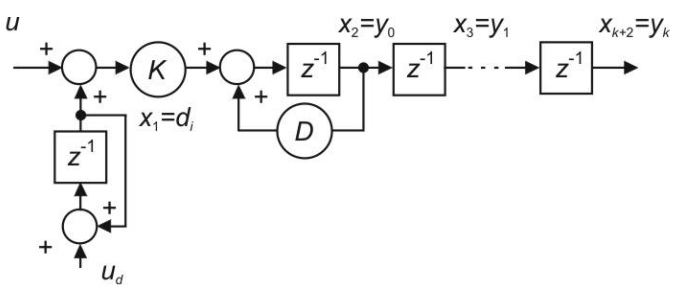
When describing one of the first published DTCs [19,20,35,36] with a stabilizing controller in the setpoint tracking channel, let us firstly suppose the nominal case with $K_m=K$ and $D_m=D$. Thereby, for the state vector (Figure 2)

$$\mathbf{x}={\left[\begin{array}{cccccc}{d}_i& y_0& y_1& y_2& \cdots & y_k\end{array}\right]}^{\prime };y_i\left(N\right)=y_0(N-i);i\in [0,k],$$

(17)

the system with a piecewise constant input disturbance $d_i=x_1=const$, actually measured output $y_0\left(N\right)=x_2$, the transport delay $T_d=k{T}_s$ and the delayed measured outputs $y_k\left(N\right)=x_{k+2}$ may be described by the following state space equations

$$\begin{array}{ccc}\hfill \mathbf{x}\left(N+1\right)& =& \mathbf{Ax}\left(N\right)+\mathbf{b}u\left(N\right)+{\mathbf{b}}_d{u}_d\left(N\right);y\left(N\right)={\mathbf{c}}^{\prime }\mathbf{x}\left(N\right);\hfill \end{array}$$

(18)

$\mathbf{A}=\left[\begin{array}{cccccc}1& 0& 0& \cdots & 0& 0\\ K& D& 0& \cdots & 0& 0\\ 0& 1& 0& \cdots & 0& 0\\ ⋮& ⋮& ⋮& \cdots & ⋮& ⋮\\ 0& 0& 0& \cdots & 1& 0\end{array}\right];\mathbf{b}=\left[\begin{array}{c}0\\ K\\ 0\\ ⋮\\ 0\end{array}\right];{\mathbf{c}}^{\prime }=\left[\begin{array}{ccc}0& \cdots & 1\end{array}\right].$

$\mathbf{A}\in {\mathit{R}}^{\left(k+2\right)\mathrm{x}\left(k+2\right)};\mathbf{b}\in {\mathit{R}}^{\left(k+2\right)\mathrm{x}1};{\mathbf{c}}^{\prime }\in {\mathit{R}}^{1\mathrm{x}\left(k+2\right)}$

Its state will be reconstructed by the Luenberger state observer [56] described as

$$\begin{array}{ccc}\hfill \overline{\mathbf{x}}\left(N+1\right)& =& \mathbf{A}\overline{\mathbf{x}}\left(N\right)+\mathbf{b}u\left(N\right)+\mathbf{h}\left(\mathbf{y}\left(\mathbf{N}\right)-{\mathbf{c}}^{\prime }\overline{\mathbf{x}}\left(\mathbf{N}\right)\right);\overline{\mathbf{y}}\left(\mathbf{N}\right)={\mathbf{c}}^{\prime }\overline{\mathbf{x}}\left(\mathbf{N}\right),\hfill \end{array}$$

(19)

which yields the observer matrix

$$\begin{array}{c}\hfill \overline{\mathbf{A}}=\mathbf{A}-\mathbf{h}{\mathbf{c}}^{\prime }.\end{array}$$

(20)

The observer vector $\mathbf{h}$ may be determined according to the Ackermann formula as

$$\begin{array}{ccc}\hfill \mathbf{h}& =& \mathbf{Q}\left(\mathbf{A}\right){\mathbf{W}}^{-\mathbf{1}};\mathbf{W}=\left[\begin{array}{c}{\mathbf{c}}^{\prime }\\ {\mathbf{c}}^{\prime }\mathbf{A}\\ {\mathbf{c}}^{\prime }{\mathbf{A}}^{\mathbf{2}}\\ ⋮\\ {\mathbf{c}}^{\prime }{\mathbf{A}}^{\mathbf{k}}\\ {\mathbf{c}}^{\prime }{\mathbf{A}}^{\mathbf{k}+\mathbf{1}}\end{array}\right]=\left[\begin{array}{ccccccc}\mathbf{0}& \mathbf{0}& \mathbf{0}& \cdots & \mathbf{0}& \mathbf{0}& \mathbf{1}\\ \mathbf{0}& \mathbf{0}& \mathbf{0}& \cdots & \mathbf{0}& \mathbf{1}& \mathbf{0}\\ \mathbf{0}& \mathbf{0}& \mathbf{0}& \cdots & \mathbf{1}& \mathbf{0}& \mathbf{0}\\ ⋮& ⋮& ⋮& ⋮& \cdots & ⋮& ⋮\\ \mathbf{0}& \mathbf{1}& \mathbf{0}& \cdots & \mathbf{0}& \mathbf{0}& \mathbf{0}\\ \mathbf{K}& \mathbf{D}& \mathbf{0}& \cdots & \mathbf{0}& \mathbf{0}& \mathbf{0}\end{array}\right],\hfill \end{array}$$

(21)

where, for $K\ne 0$, $\mathbf{W}$ is a regular observability matrix. For a dead-beat observer, when $Q\left(z\right)=z^{k+1}$, we obtain

$$\begin{array}{ccc}\hfill \mathbf{h}& =& \left[\begin{array}{c}1/K\\ 1+D+...+D^{k+1}\\ 1+D+...+D^k\\ ⋮\\ 1+D\end{array}\right]=\left[\begin{array}{c}1/K\\ (D^{k+2}-1)/(D-1)\\ (D^{k+1}-1)/(D-1)\\ ⋮\\ 1+D\end{array}\right].\hfill \end{array}$$

(22)

From such a dead-beat reconstruction we may then easily introduce both the delay and disturbance compensations with a required filtration degree, or implement a control with dynamical setpoint feedforward.

This early state-space-inspired solution, for state and disturbance reconstruction and control, has been used on the simplest integrating models ($a=0$), as well as on static (stable and unstable) models with $a\ne 0$. At about the same time, a similar solution, today known as Extended State Observer (ESO), has been proposed by [39]. It is focusing on design based on integrating models (in our case with $a_m=0$), which is specific for the Active Disturbance Rejection Control (ADRC). However, the solutions dealing with time-delayed first-order systems under the ADRC brand (see, for example [5,6]) came much later than the above-described proposal.

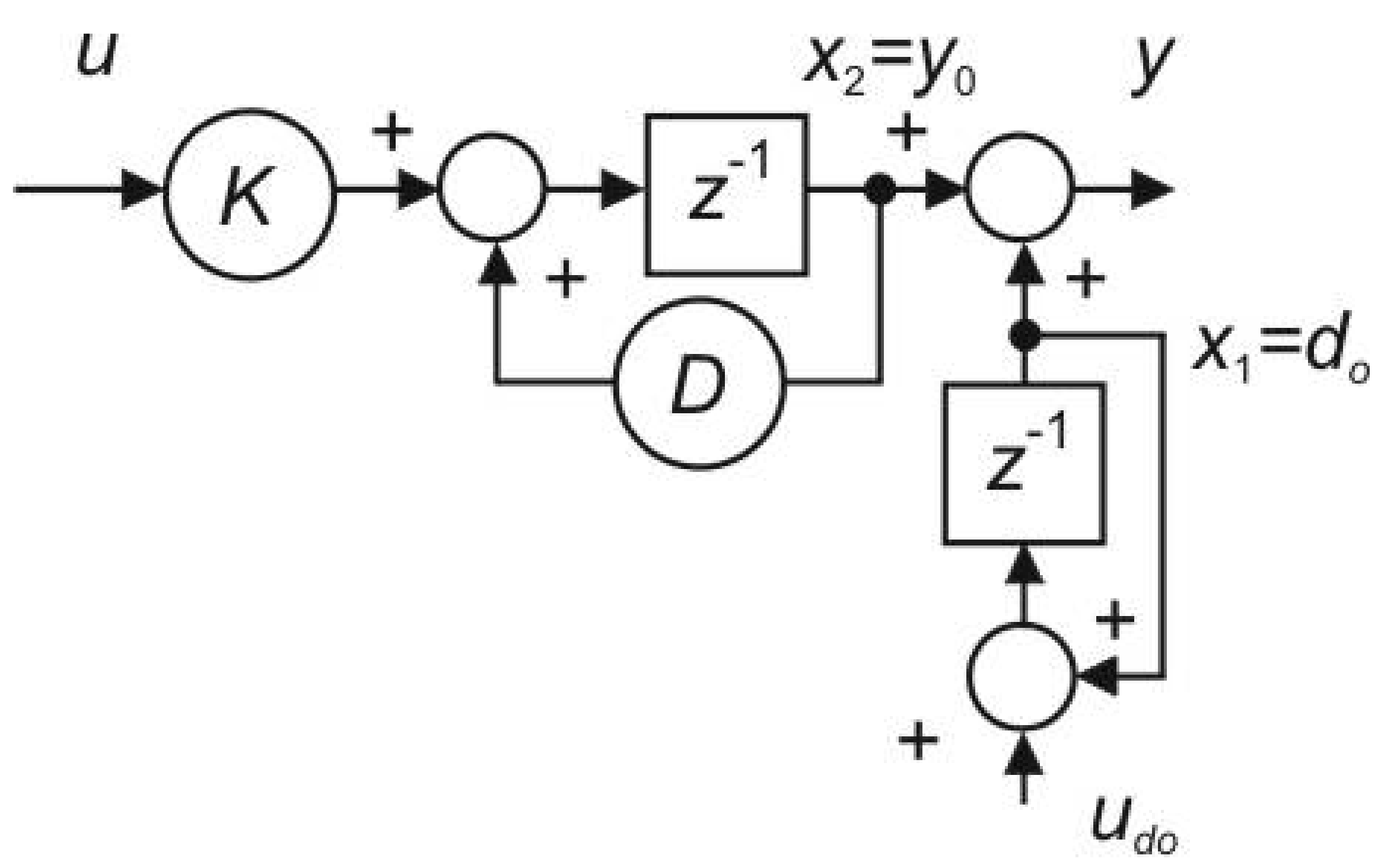
2.6. Why Not the Output Disturbance Reconstruction?

On the other hand, in a case of a piecewise constant output disturbance $d_o$ (Figure 3), it may be shown that even for a delay-free plant ($k=0$), with respect to

$$\mathbf{A}=\left[\begin{array}{cc}1& 0\\ 0& D\end{array}\right];\mathbf{b}=\left[\begin{array}{c}0\\ K\end{array}\right];{\mathbf{c}}^{\prime }=\left[\begin{array}{cc}1& 1\end{array}\right];\mathbf{W}=\left[\begin{array}{c}{\mathbf{c}}^{\prime }\\ {\mathbf{c}}^{\prime }\mathbf{A}\end{array}\right]=\left[\begin{array}{cc}\mathbf{1}& \mathbf{1}\\ \mathbf{1}& \mathbf{D}\end{array}\right],$$

(23)

such a configuration is unobservable for $D=1$. Hence, for integrating plant models it makes no sense to reconstruct and compensate output disturbances. If anyone has to use such a control scheme based on unobservable signals, the scheme has to be modified by eliminating the unobservable signal from the implementation scheme. Thus, by modifying the original structure, it can be applied, but without the reconstruction of the output disturbance. In addition, the output disturbance $d_o$, equivalent, for integrating plants, to $d_i=const$, increases over time beyond all limits, leading to overflow of the computer’s registers. As a result, the first DTCs focused on the reconstruction and compensation of input disturbances.

2.7. Polynomial Interpretation of ESO-Based Non-Delayed Signals Reconstruction

While the state-space approach is useful for the initial analysis and design yielding the observer and controller structure, for interpretation of the mentioned approaches and a modified use, it is easier to deal with a polynomial approach. From the observer Equation (19), rewritten as

$$\overline{\mathbf{x}}\left(z\right)={\left(z{\mathbf{I}-\mathbf{A}+\mathbf{hc}}^{\prime }\right)}^{-1}[\mathbf{b}u+\mathbf{h}y\left(z\right)],$$

(24)

it is possible to express the reconstructed actual plant output $y_0$ and the input disturbance $d_i$ as:

$${\overline{y}}_0\left(N\right)=\left[\begin{array}{cccc}0& 1& \cdots & 0\end{array}\right]\overline{\mathbf{x}}\left(N\right);{\overline{d}}_i\left(N\right)=\left[\begin{array}{cccc}1& 0& \cdots & 0\end{array}\right]\overline{\mathbf{x}}\left(N\right).$$

(25)

Taking into account expression (24), Equation (25) yields

$$\begin{array}{l}{\overline{y}}_0\left(N\right)=S_{uy}\left(z\right)u\left(N\right)+S_{yy}\left(z\right)y\left(N\right);\hfill \\ S_{uy}\left(z\right)={\displaystyle \frac{K(z-1)[z^k+{\beta }_{k-1}{z}^{k-1}+...+{\beta }_0]}{z^{k+2}}};S_{yy}\left(z\right)={\displaystyle \frac{{\alpha }_{1}z+{\alpha }_0}{z^2}};\hfill \\ {\beta }_{k-1}=1+D;{\beta }_{k-2}=1+D+D^2;{\beta }_0=1+D+D^2+...+D^k={\displaystyle \frac{D^{k+1}-1}{D-1}};\hfill \\ {\alpha }_1=1+D+...+D^{k+1}={\displaystyle \frac{D^{k+2}-1}{D-1}};{\alpha }_0=-(D+...+D^{k+1})=-D{\displaystyle \frac{D^{k+1}-1}{D-1}};\\ {\overline{d}}_i\left(N\right)=S_{ud}u\left(N\right)+S_{yd}y\left(N\right);\\ S_{ud}\left(z\right)=-{\displaystyle \frac{1}{z^{k+2}}};S_{yd}\left(z\right)={\displaystyle \frac{z-D}{K{z}^2}}.\end{array}$$

(26)

Given the maximum overall delay $k_t=k+2$ occurring in these relationships, it can be stated that the proposed dead-beat responses based on Equation (26) can be ideally completed in $k_t$ steps.

2.8. Controller Design for the Shortest Possible Transient Responses

The relationships (26) can also be derived by a much simpler polynomial approach, and, at the same time, use higher flexibility in determining the order of individual transfer functions, which is used by the DOB-based approach initiated in [57,58] and for the time-delayed systems applied in [46].

The input disturbance reconstruction (see Figure 4) can be based on the formula

$${\overline{d}}_i=u_a-u.$$

(27)

Using the inverse transfer function of the system, $u_a$ can be formally expressed as $u_a=S{\left(z\right)}^{-1}y$, which yields

$${\overline{d}}_i\left(N\right)={\displaystyle \frac{(z-D)z^k}{K}}y\left(N\right)-u\left(N\right).$$

(28)

By modifying this non-causal relationship, the fastest achievable causal estimate of the input disturbance $d_i$ corresponds to its value delayed by $k+1$ steps, expressed as

$${\overline{d}}_i(N-k-1)={\displaystyle \frac{(z-D)}{Kz}}y\left(N\right)-\frac{1}{z^{k+1}}u\left(N\right).$$

(29)

Hence, the polynomial interpretation of the disturbance reconstruction including the inverse plant model $S_0{\left(z\right)}^{-1}$ (in $S_{yd}\left(z\right)$) is quite simple and fully equivalent to the continuous case presented in [46]. The disturbance ${\overline{d}}_i$ delayed equally as the measured plant output may then be simply calculated by subtracting the equally delayed controller output from the reconstructed plant input signal [45,46]. Similarly as in [59], with respect to ESO, the DOB-reconstruction delay may be decreased by one step to $k_t=k+1$ steps.

In addition, the reconstruction of the actual plant output $y_0$ can be interpreted by solving the Diophantine equation resulting from an intuitive requirement of behaviour equivalent to delay-free plant [19,20]: the signal ${\overline{y}}_0$ resulting from the introduced feedback should be equivalent to the undelayed plant output $y_0$. Therefore, with respect to the control signal u it must hold

$${\displaystyle \frac{{\overline{y}}_0}{u}}=S\left(z\right)S_{yy}\left(z\right)+S_{uy}\left(z\right)=S_0\left(z\right).$$

(30)

Thereby, in order to make the output reconstruction independent from a constant disturbance $d_i$, the transfer function $S_{uy}\left(z\right)$ has to include factor $z-1$ in its numerator (the effect of feedback through $S_{uy}$ will depend on the difference of two consecutive input values, where the constant value $d_i$ does not apply).

Note that a modification of the ESO solution (26), Equation (30) may also be expressed in the form

$${\displaystyle \frac{K}{(z-D)z^{k+2}}}\left[{\alpha }_{1}z+{\alpha }_0+(z-1)(z-D)(z^k+{\beta }_{k-1}{z}^{k-1}+...+{\beta }_0)\right]={\displaystyle \frac{K}{z-D}}.$$

(31)

From Equation (31) follows

$${\alpha }_{1}z+{\alpha }_0+(z-1)(z-D)(z^k+{\beta }_{k-1}{z}^{k-1}+...+{\beta }_0)=z^{k+2}.$$

(32)

Comparison of the coefficients at the individual powers of z in Equation (32) with ${\beta }_k=1$ yields two systems of equations. The first one with a triangular matrix and ${\beta }_k=1$

$$\begin{array}{c}\left[\begin{array}{ccccccccc}1& 0& 0& 0& ...& 0& 0& 0& 0\\ -(1+D)& 1& 0& 0& ...& 0& 0& 0& 0\\ D& -(1+D)& 1& 0& ...& 0& 0& 0& 0\\ ⋮& ⋮& ⋮& ⋮& ...& ⋮& ⋮& ⋮& ⋮\\ 0& 0& 0& 0& ...& -(1+D)& 1& 0\\ 0& 0& 0& 0& ...& D& -(1+D)& 1\end{array}\right].\left[\begin{array}{c}{\beta }_k\\ {\beta }_{k-1}\\ {\beta }_{k-2}\\ ⋮\\ {\beta }_1\\ {\beta }_0\end{array}\right]=\left[\begin{array}{c}1\\ 0\\ 0\\ ⋮\\ 0\\ 0\end{array}\right]\hfill \end{array}$$

(33)

has the solution

$$\begin{array}{c}{\beta }_{k-1}=(1+D){\beta }_k=1+D\hfill \\ {\beta }_{k-2}=(1+D){\beta }_{k-1}-D{\beta }_k=1+D+D^2\hfill \\ ⋮\hfill \\ {\beta }_0=(1+D){\beta }_1-D{\beta }_2=1+D+...+D^k={\displaystyle \frac{D^k-1}{D-1}}.\hfill \end{array}$$

(34)

From the second subsystem of equations

$$\begin{array}{c}\left[\begin{array}{cc}D& -(1+D)\\ 0& D\end{array}\right].\left[\begin{array}{c}{\beta }_1\\ {\beta }_0\end{array}\right]+\begin{array}{c}\left[\begin{array}{cc}1& 0\\ 0& 1\end{array}\right].\left[\begin{array}{c}{\alpha }_1\\ {\alpha }_0\end{array}\right]=\left[\begin{array}{c}0\\ 0\end{array}\right]\hfill \end{array}\hfill \end{array}$$

(35)

follows

$$\begin{array}{c}{\alpha }_1=(1+D){\beta }_0-D{\beta }_1=1+D+...+D^{k+1}={\displaystyle \frac{D^{k+2}-1}{D-1}};\hfill \\ {\alpha }_0=-D{\beta }_0=-D(1+D+...+D^k)=-D{\displaystyle \frac{D^{k+1}-1}{D-1}}.\hfill \end{array}$$

(36)

However, similarly as in disturbance reconstruction, the polynomial approach offers flexibility also in reconstruction of the actual output $y_0$. Equations (31)–(36) can be resolved for a reduced minimal feasible delay $k_t=k+1$, thus reducing the number of steps required to reconstruct the current output. The corresponding transfer functions are:

$$\begin{array}{c}{S}_{uy}\left(z\right)={\displaystyle \frac{K(z-1)[z^{k-1}+{\beta }_{k-2}{z}^{k-2}+...+{\beta }_0]}{z^{k+1}}};\hfill \\ {\beta }_{k-2}=1+D;{\beta }_{k-3}=1+D+D^2;...{\beta }_0={\displaystyle \frac{D^k-1}{D-1}};\hfill \\ S_{yy}\left(z\right)={\displaystyle \frac{{\alpha }_{1}z+{\alpha }_0}{z}};{\alpha }_1={\displaystyle \frac{D^{k+1}-1}{D-1}};{\alpha }_0=-D{\displaystyle \frac{D^k-1}{D-1}};\hfill \\ S_{ud}\left(z\right)=-{\displaystyle \frac{1}{z^{k+1}}};S_{yd}\left(z\right)={\displaystyle \frac{z-D}{Kz}}.\end{array}$$

(37)

For the system in Figure 2, based on measuring the plant input and output with an additional filtration (with $F\left(z\right)$ (Equation (13)) defined as $F=NQ/DQ$), it possible to compile a simple scheme for the reconstruction of any of the internal variables, i.e., also the actual system output $y_0$ and its input disturbance $d_i$ (Figure 5).

2.9. Filtration Aspects—PrP-DOB Controller

Reconstruction of the input disturbance $d_i$ and the non-delayed output $y=y_0$ enables their further use within the circuit in Figure 5 inspired by Figure 1. Such a procedure, which employs simple relationships, and requires only selection of n and $\lambda$ and the calculation of $K_P$ (Equation (16)), seems more appropriate than perpetual change of the characteristic observer polynomial in Equation (21) to achieve the required filtration and then recalculation of $K_P$. With respect to elimination of delay in the output and disturbance reconstruction, including use of disturbance observer (DOB), this controller will be denoted as predictive P controller (PrP) with DOB-based disturbance reconstruction and compensation, shortly PrP-DOB controller.

2.10. Example 1

To illustrate the different possible areas of application of the proposed PrP-DOB controller and its settings, let us first consider the plant with nominal model parameters ${\overline{K}}_s=K_s=1$, $\overline{a}=a=-1$, $T_d=0.6$. This relative dead time value $T_d/T=0.6,T=1/\left|a\right|$ is significantly larger than $T_d/T=0.19$ used in an unstable chemical reactor discussed in [14] and by some other contributions to SP modifications for unstable plants. Four different tuning scenarios have been proposed:

• Dead-beat performance without additional filtration ($n=0$)—appropriate only for relatively long sampling periods (the chosen value $T_s=0.2$ gives $k=3$) and a relatively low measurement noise and model uncertainty. For $T_c\to 0$ we get $D_c=0$ and $K_p=5.5167$ (Equation (11)). This setting is important for comparing the results of the original state-space and reduced polynomial approaches;
• Transients with relatively long sampling periods ($T_s=0.2$), slowed down by selection of $T_c=1$, which is reflected in the value of the pole $D_c=0.8187$ and the reduced gain $K_p=1.8187$. This can partially reduce the effect of noise and circuit uncertainties also without an additional filtration;
• A significant increase of noise attenuation and robustness to uncertainties can only be achieved with shorter sampling periods. For larger ones, the additional filtration would threaten the stability of the control system with unstable plant. By choosing $T_s=0.01$, $n=1$ and $T_f=0.1$ yielding $\lambda =e^{-T_s/T_f}=0.9048$, we obtain $K_p=2.8936$ (Equation (16));
• A further increase in damping and robustness can be achieved by using higher-order filters, e.g., $n=2$ with $T_s=0.01$, $T_f=0.1$, $\lambda =0.9048$ and $K_p=1.8958$.

The corresponding transients are given in Figure 6. Obviously, decreasing the controller order and choosing shorter sampling period is beneficial in terms of the disturbance response for long $T_s$ without additional filtration. For the shorter sampling periods with filtration applied, the difference in the total considered delay ($k_t=k+2$ or $k_t=k+1$) is not to distinguish in the plant output and input responses, but may be important for the reconstructed disturbance response using higher-order filters.

2.11. Summary 1

Setting up the PrP-DOB controller depends on filtration. Without additional filtration, the gain $K_p$ is set by changing the parameter (required closed loop time constant) $T_c$, or the corresponding pole $D_c$. When using an additional filter, the parameters $T_c$, or $D_c$ may not be chosen independently. Instead, $K_p$ is calculated from the selected filter order n and its time constant $T_f$. The only difference between stable, integrating and unstable systems is that in the case of unstable systems it is not possible to choose arbitrarily large filter time constant and/or the sampling period. The dependence of the transients on the (possibly uncertain) setting parameters can be easily verified using the web application at http://apps.iolab.sk/advanced/mathematics2021/, accessed on 25 June 2021.

The reconstruction of output and input disturbances could also be further modified for the purpose of dynamic feedforward control within the so-called reference model control [18,60]. However, in this paper, before giving a practical demonstration of the algorithms, we are going to briefly discuss the modification of the discrete-time FSP according to [21,22].

3. Smith Predictor Inspired Controllers

If we want to explain all the conditions for successful application of Smith predictor inspired solutions, we need to start from the feedforward control dynamics [17,18]. The possibility of a discrete-time feedforward control by the closed-loop P controller immediately follows from $F_{wu}\left(z\right)$ in Equation (12).

However, let us firstly note that such an interpretation is far from common. In one of the basic contemporary control textbooks [61], the feedforward control and the Smith predictor have been presented in two completely independent chapters, without discussing their interrelationships. It indicates that these two problems are not generally known as related to each other. The same holds for numerous works on the so-called Filtered Smith predictor (FSP) published before 2013. There is no term “feedforward” in article [14] either. Thus, the third SP interpretation denoted as “Dynamical setpoint feedforward and output disturbance rejection” may present a new information for the readers. Therefore, it deserves a deeper attention. Furthermore, we believe that it has also never been mentioned that the FSP structure has the following deficiencies:

• Unobservable output disturbances $d_o$ for integrating models;
• Unlimited $d_o$ increase for unstable and integrating plant models corresponding to external or internal input disturbances;
• The problems in the presence of control constraints.

It is worth to mention that the authors of [14] added a note that the proposed schemes needed to be further modified for implementation. However, they did not sufficiently explain, why and how, and that such a change completely changes the functionality of the structure, which no longer has the ability to provide a reconstructed disturbance signal.

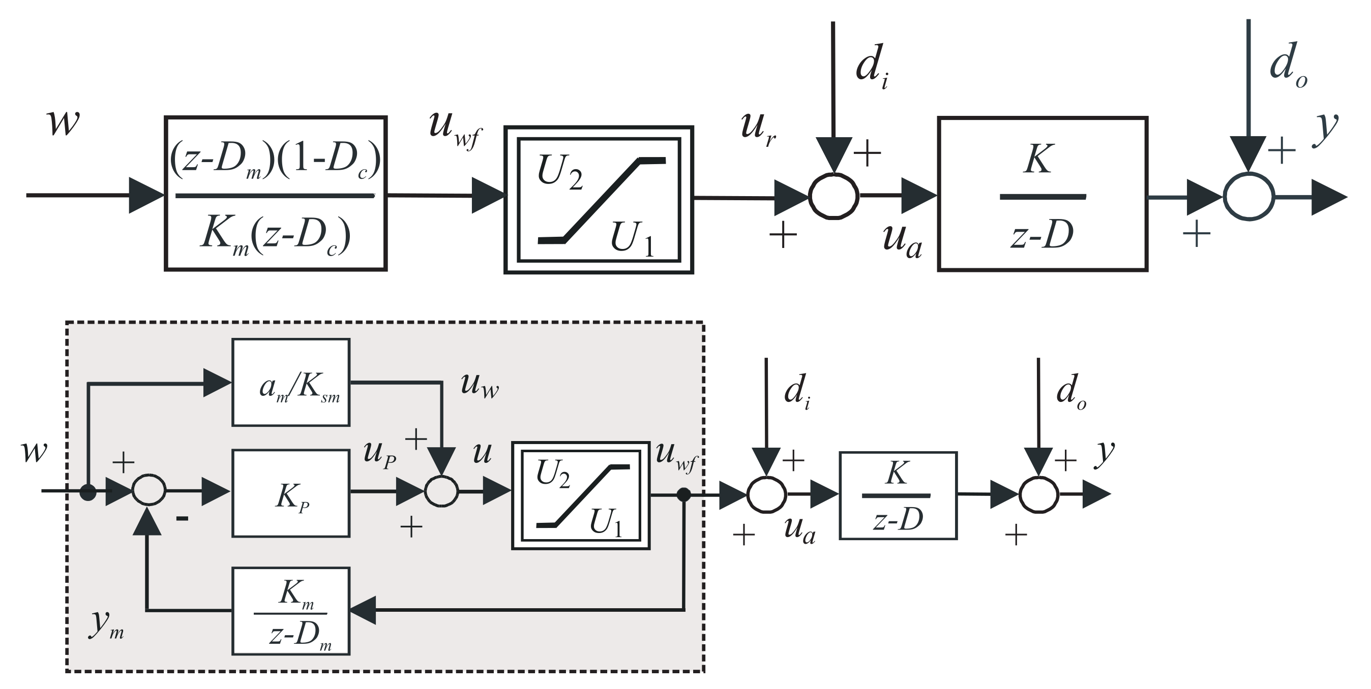
3.1. SP Structure for Constrained Control

If a feedforward has to deal effectively with impact of the control signal constraints, which are especially relevant when controlling unstable systems, its implementation by the transfer functions (5) and (6) does not represent the optimal solution. Instead, a much more effective approach is to use a primary loop (as illustrated for the continuous-time control by transients in [18]) with plant models (1)–(3) and a constrained P controller set in the continuous- and discrete-time-domains as (see Figure 7)

$$\begin{array}{c}{K}_P=(1/T_c-a_m)/K_{sm}\hfill \\ K_P=(D_m-D_c)/K_m;D_c=e^{-T_s/T_c}\hfill \end{array}$$

(38)

In the proportional zone of control, the primary loop yields the controller transfer function (5). Then, unlike the feedforward implementation by the filtered inversion by the model transfer function, it also takes into account the control signal limitations for the inverse dynamics [21,22]. Therefore, without constraints, there are no reasons to use the feedforward implementation in form of the primary loop. Hence, there are no reasons for using the traditional SP structure for linear systems. Surprisingly, in the large majority of papers devoted to SP and its modifications there are no comments mentioning the constraints. The proper realization of constrained feedforward control deals with a conditioning technique ([62], pp. 737).

Furthermore, the traditional solutions with PI control exhibit in such situations windup and make the tuning rules for different plant types unnecessarily complex [63,64,65,66,67]. These are fundamental, not sufficiently emphasized shortcomings of the traditional SP in the existing literature, which neglects the realization of an inverse dynamics by means of control. The fact that each controller [68] inherently includes the inverse plant model is known for a long time. It is then not necessary to use such complex solutions as proposed in [60].

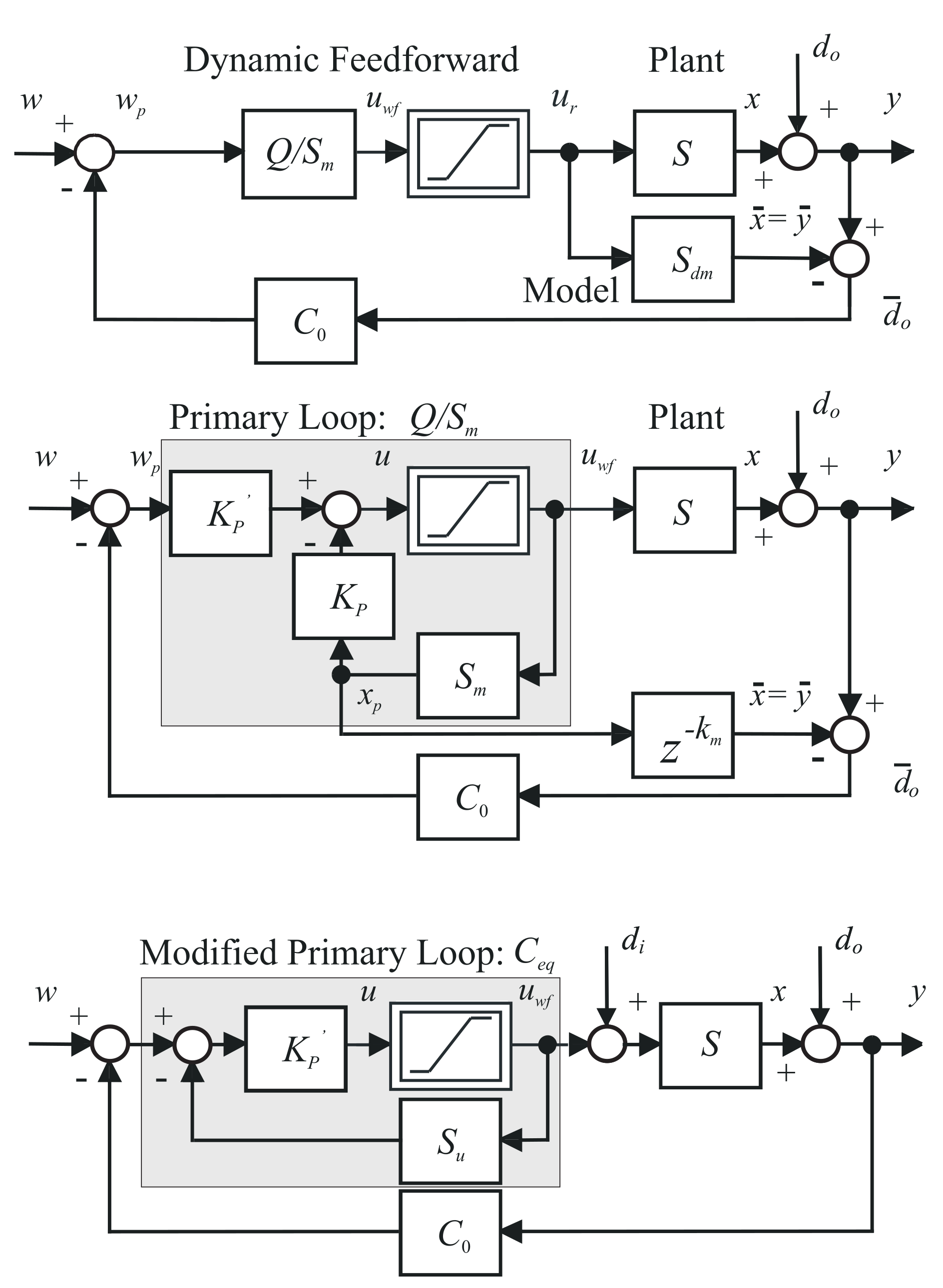
3.2. 2-DoF SP with a Stabilizing Disturbance Feedforward

Here, it will be shown, how the reference setpoint feedforward may be extended by reconstruction and compensation of non-measurable output disturbances using IMC structure with a parallel model, as given in Figure 8.

Moreover, in the case of unstable control systems, there is another strong argument for the feedforward control implementation by the primary loop that was not required in SPs for stable systems: In the transfer-functions-based IMC control with parallel plant model (as in Figure 8), one control action cannot stabilize, even identical, two parallel unstable systems. In order to extend this structure to integrating and unstable systems, the model $S_m$ has to be embedded in the (stabilizing) primary loop. In addition, in order to apply feedforward control to unstable plants (see Equation (7)), it is also necessary to stabilize their input disturbance response (by the structure called as 2-DoF SP) with the feedback controller $C_o$, which does not modify the primary loop dynamics. With respect to the properties of unstable plants, discussed in Section “Model uncertainties and setpoint feedforward”, the disturbance feedback provides zero total disturbance at the plant input. Therefore, to eliminate the (possibly unstable) plant dynamics from the disturbance response, $C_o$ composed of a stabilizing PD control

$$R_{fb}\left(z\right)=1+{\beta }_n(z-1),$$

(39)

combined with an $n\ge 1$ order low-pass filter ${(1-D_f)}^n/{(z-D_f)}^n;D_f=e^{-\frac{T_s}{T_f}}$ with a unity steady-state gain, a proper transfer function, and yields disturbance feedforward (to keep the number of tuning parameters as low as possible, the disturbance feedforward will mostly use the same time constant $T_f=T_c$ as introduced for the primary loop tuning)

$$\begin{array}{c}{C}_o\left(z\right)={\left({\displaystyle \frac{1-D_f}{z-D_f}}\right)}^n\left[1+{\beta }_n(z-1)\right].\hfill \end{array}$$

(40)

In [21,22] the low pass filter order in $C_o$ has been chosen just with respect to properness. Since the first-order filter may be associated with high noise exposure, some authors (e.g., [14]) start with evaluating the second-order filters, whereby they introduce $C_o$ with two unknown parameters, but without considering its unit steady-state gain.

In order to eliminate the possibly unstable plant pole $z=D=e^{-a{T}_s}$ from the nominal input disturbance response

$$\begin{array}{c}{F}_{iy}\left(z\right)=S\left(z\right)\left(1-Q\left(z\right)C_o\left(z\right)z^{-k}\right)\hfill \end{array}$$

(41)

the parameter ${\beta }_n$ has to be chosen as

$$\begin{array}{c}{a}_m=0;{\beta }_n=k+{\displaystyle \frac{1}{1-D_c}}+{\displaystyle \frac{n}{1-D_f}};D_f=e^{-T_s/T_f};D_c=e^{-T_s/T_c};n=1,2,...\hfill \\ a_m\ne 0;{\beta }_n={\displaystyle \frac{1-D^k{\displaystyle \frac{D-D_c}{1-D_c}}{\left({\displaystyle \frac{D-D_f}{1-D_f}}\right)}^n}{1-D}};D=e^{-a_m{T}_s}\hfill \end{array}$$

(42)

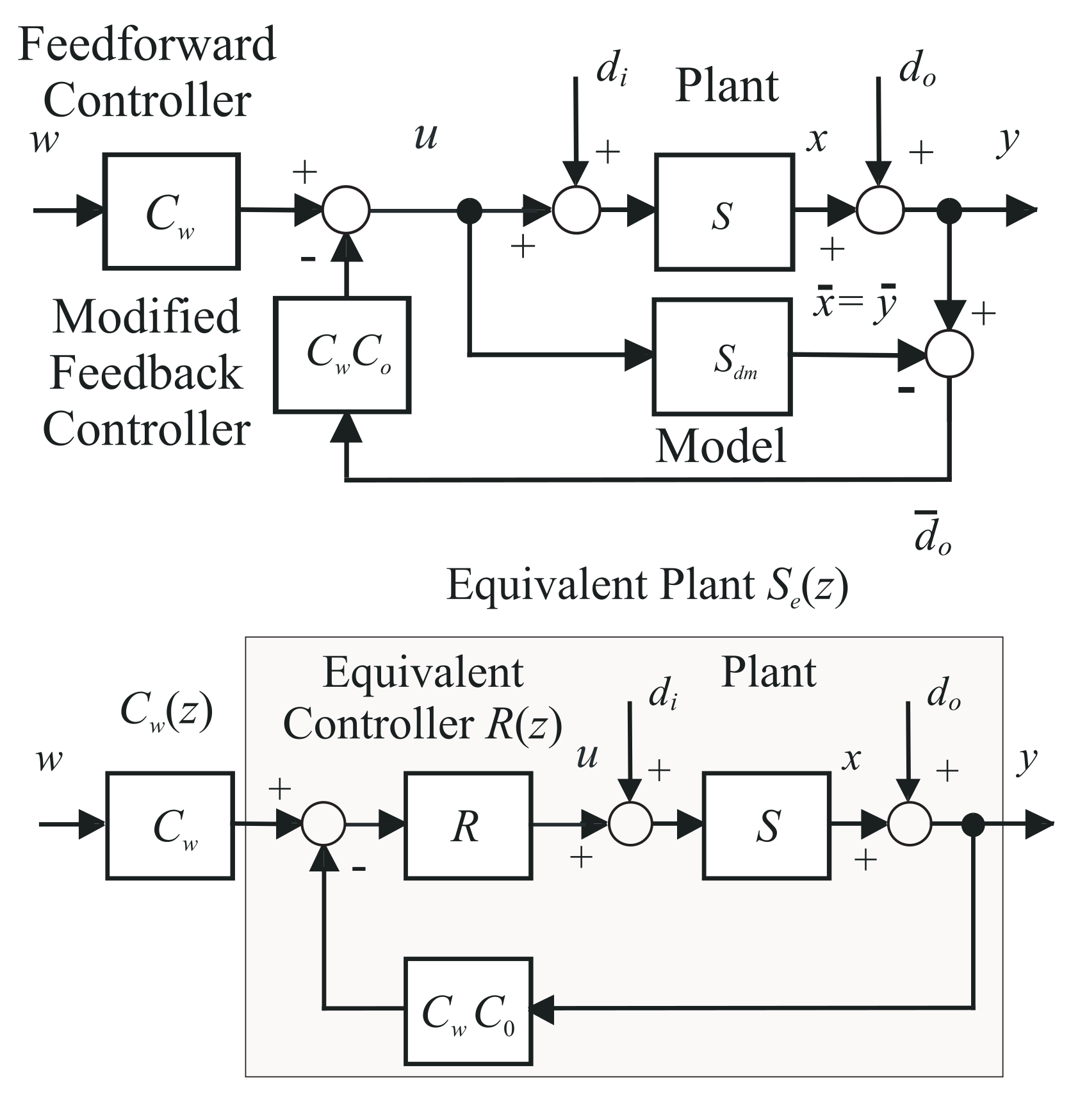
3.3. Loop Stability Versus Disturbance Response Stability

As in each disturbance observer-based control [44], disturbance feedforward makes the controlled plant to behave as the nominal model $S_m\left(z\right)$ and thus achieves invariance of the considered control to the model uncertainty. When replacing the internal positive feedback through the plant model $S_{dm}$ and the blocks $C_w\left(z\right)C_o\left(z\right)$ in Figure 9, the equivalent controller $R\left(z\right)$ is

$$\begin{array}{c}R\left(z\right)={\displaystyle \frac{1}{1-S_m{z}^{-k_m}{C}_{o}Q{S}_m^{-1}}}={\displaystyle \frac{1}{1-Q{C}_o{z}^{-k_m}}}\hfill \end{array}$$

(43)

Together with the plant $S\left(z\right)$ and the blocks $C_w\left(z\right),C_o\left(z\right)$ yields the equivalent plant dynamics $S_e\left(z\right)$

$$\begin{array}{c}{S}_e\left(z\right)={\displaystyle \frac{S_{m}S}{S_m(1-Q{C}_o{z}^{-k_m})+Q{C}_{o}S}}\hfill \end{array}$$

(44)

connected in series with the setpoint feedforward $C_w\left(z\right)$. The corresponding input disturbance response is

$$\begin{array}{c}{F}_{iy}\left(z\right)={\displaystyle \frac{S}{1+S{C}_w{C}_{o}R}}={\displaystyle \frac{S{S}_m(1-Q{C}_o{z}^{-k_m})}{S_m(1-Q{C}_o{z}^{-k_m})+Q{C}_{o}S}}\hfill \end{array}$$

(45)

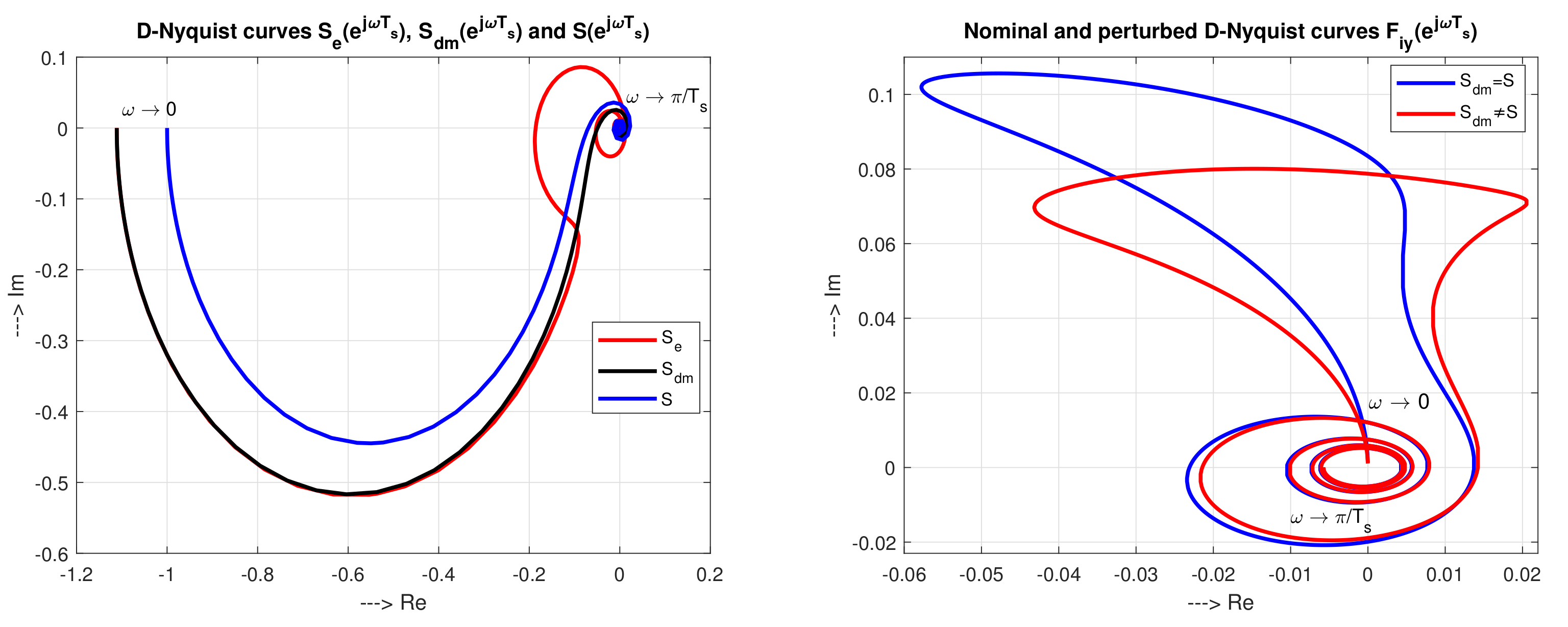
For relatively low frequencies $\omega \to 0$, when according to $z=e^{j\omega T}\to 1$ and $C_o\left(z\right)Q\left(z\right)z^{-k_m}\to 1$, $S_e\left(z\right)$ approaches the model dynamics $S_m\left(z\right)$ (Equation (46)) (see Figure 10). From $F_{iy}\left(1\right)=0$, it follows that for stable plants the loop guarantees full compensation of constant disturbances in steady state. Similarly, as in the case of compensation of input disturbances by disturbance observer [44], the following limit cases hold:

$$\begin{array}{c}z\to 1,C_o\left(z\right)Q\left(z\right)z^{-k_m}\to 1,S_e\left(1\right)\approx S_m\left(z\right),F_{iy}\left(z\right)=0\hfill \\ z\to \infty ,C_o\left(z\right)Q\left(z\right)z^{-k_m}\to 0,S_e\left(z\right)\approx S\left(z\right)\hfill \end{array}$$

(46)

At high frequencies, when $C_o\left(z\right)Q\left(z\right)z^{-k_m}\to 0$, the disturbance feedforward loses its effectiveness and $S_e\left(z\right)$ behaves as an uncontrolled plant $S\left(z\right)$.

These features, applied now to the structures based on setpoint feedforward combined with output disturbance compensation from Figure 9, may well be documented by the corresponding Nyquist curves (Figure 10). It needs to be emphasized that they lead to conflicting requirements, when with regard to the stability of the plant state, it is not possible to impose the compensation dynamics corresponding to an unstable model, but with respect to the aptness of the reconstruction, we obtain the best short term results with unstable model approximating optimally the controlled dynamics. It also led to the incorrect conclusions that the stability of disturbance responses was considered to be sufficient condition for the stability of the system state. However, this is not true, as will be shown in the following sections.

3.4. Why the Structure of FSP and Not a Compact Equivalent Controller?

Despite several modifications to the Smith predictor were suggested so far in order to control unstable systems, which are based on the above analysis, they are still not sufficient to ensure stability of the circuit in Figure 8 (middle). When being aware of the fact that the output disturbance, which is used for reconstruction, is unobservable in the case of integrating systems and that it grows infinitely due to possible constant input disturbances on unstable plants, it is straightforward that the mentioned structure is not applicable. Therefore, it is clear that the reconstruction of output disturbance should be avoided. However, the scheme can be modified so that at least some of its functional advantages related to the limitation of the control signal remain unchanged. Figure 8 below depicts such a modification, which may be fully equivalent to the structure presented in the middle with respect to the input and output signals of the saturation u and $u_{wf}$. In other words, the local feedback around the saturation (including $S_m$ and $K_P$) has to be united with the feedback including $z^{-k_m}$ and $C_o$ into the new block

$$S_u\left(z\right)=S_m\left(z\right)[{\displaystyle \frac{K_P}{K_P^{\prime }}}-C_o\left(z\right)z^{-k_m}]={\displaystyle \frac{N_{Su}\left(z\right)}{D_{Su\left(z\right)}}}$$

(47)

Such a solution avoids the unbounded output disturbance reconstruction, which could lead to overflow of computer registers.

As mentioned in [14], for a stabilizing disturbance feedforward $C_o\left(z\right)$, with ${\beta }_n$ (Equation (42)) calculated to cancel the unstable plant pole $z=D$ from the disturbance transfer function $H_{iy}\left(z\right)$, the unstable pole will also be canceled from Equation (47) and the controller will be based on internally stable blocks. From the user’s point of view, however, not only the calculation of ${\beta }_n$ parameters is important, but also the calculation of the stable transfer function (47), where the value of $k_m$ can be high for short sampling periods $T_s$. Since the derivation of $S_u$ is missing in [14] and its expression is not trivial, we will derive it here by using several approaches.

3.5. Integrating Plants

In the special case of integrating plant models with $a_m=0$, $K_P^{\prime }=K_P$ and unobservable output disturbances, besides of eliminating the pole $z=1$ [22] in

$$\begin{array}{c}{F}_{iy}\left(z\right)={\displaystyle \frac{S\left(z\right)}{1+K_P{S}_0\left(z\right)}}\left[1-{\displaystyle \frac{C_o\left(z\right)}{z^k}}\right]={\displaystyle \frac{N_{Fiy}\left(z\right)}{D_{Fiy}\left(z\right)}}\hfill \end{array}$$

(48)

it is also necessary to eliminate the reconstructed output disturbance ${\overline{d}}_o$ from the 2-DoF SP control scheme in Figure 8 (middle), according to the bottom scheme. Thus, in order to get a zero steady-state error, it must not only hold that $F_{iy}\left(1\right)=0$, but the numerator $N_{Fiy}\left(z\right)$ must have a double zero $z=1$ to also cancel the pole $z=1$ brought by the step transform $z/(z-1)$.

Secondly, in order to avoid using ${\overline{d}}_o$, but still keeping the unmodified control algorithm used for calculating the control signal (avoiding problems with control constraints [22]), one may use a loop with all internal feedbacks from the saturated controller output into block $S_u$ of the equivalent controller denoted usually as FSP. As discussed in [17,22], this controller can no longer be interpreted as a dynamic feedforward with output disturbance reconstruction and compensation—the reconstructed disturbance no longer occurs in the controller structure, in which neither feedforward can be identified. Therefore, the name used is misleading. Rather, it would be appropriate to talk about the SP-inspired solutions.

Introduction of this block, with or without further simplification of the loop by an equivalent controller $K_P/(1+K_P{S}_u)$ [21], cannot be reliably accomplished without taking into account the limitations of the control action.

In the nominal case and in addition to the calculation ${\beta }_n$, according to Equation (42), it is yet necessary to calculate $S_u\left(z\right)$ (Equation(47)). For the nth order denominator of $C_o\left(z\right)$, given by Equation (40), the numerator coefficients

$$N_{Su}\left(z\right)=f_0+...+f_{n+k}{z}^{n+k-1}$$

(49)

represent the remainder after dividing the numerator of $N_{su}\left(z\right)$ (Equation (47)) with $D_{su}\left(z\right)$ yielding

$$\begin{array}{c}G\left(z\right)=K{z}^k{(z-D_c)}^n-K[1+{\beta }_n(z-1)]{(1-D_c)}^n=\hfill \\ =g_0+g_{1}z+...+g_{n+k}{z}^{n+k};\hfill \end{array}$$

(50)

It means that they follow from equation

$$N_{Su}\left(z\right)(z-1)=G\left(z\right)$$

(51)

$$\begin{array}{c}\left[\begin{array}{cccccc}1& 0& 0& 0& ...& 0\\ -1& 1& 0& 0& ...& 0\\ 0& -1& 1& 0& ...& 0\\ ⋮& ⋮& ⋮& ⋮& ...& ⋮\\ 0& 0& 0& 0& ...& 1\\ 0& 0& 0& 0& ...& -1\end{array}\right].\left[\begin{array}{c}{f}_{n+k-1}\\ f_{n+k-2}\\ ⋮\\ f_1\\ f_0\end{array}\right]=\left[\begin{array}{c}{g}_{n+k}\\ g_{n+k-1}\\ g_{n+k-2}\\ ⋮\\ g_1\\ g_0\end{array}\right]\hfill \end{array}$$

with solution

$$f_{n+k-1}=g_{n+k}=K;f_{n+k-i}=f_{n+k-i+1}+g_{n+k-i+1};-f_0=g_0;i\in [2,n+k]$$

(52)

Analytically, the solution can also be handled, preferably with the help of computer algebra (by partial fraction decomposition). Here, the formulas will be limited to the simplest cases starting with the first order $C_o\left(z\right)$ corresponding to $n=1$ in Equation (40), when $S_{un}\left(z\right)=S_u\left(z\right)$. The results for $n=1,2,3$ are the following

$$\begin{array}{c}{S}_{u1}\left(z\right)=K{\displaystyle \frac{z^k+D_1{z}^{k-1}+...+D_{1}z-(\beta -1)D_1}{(z-D_f)z^k}};\hfill \\ S_{u2}\left(z\right)=K{\displaystyle \frac{z^{k+1}+(1-2D_f)z^k+D_2{z}^{k-1}+...+D_{2}z-(\beta -1)D_2}{{(z-D_f)}^2{z}^k}};\\ S_{u3}\left(z\right)=K\frac{z^{k+2}+(1-3D_f)z^{k+1}+(1-3D_f+3D_f^2)z^k+D_3{z}^{k-1}+...+D_{3}z-(\beta -1)D3}{{(z-D_f)}^3{z}^k};\\ Dn={(1-D_f)}^2;\hspace{1em}n=1,2,3\end{array}$$

(53)

In this way, it is a relatively easy to derive the values for any integer k and higher values of n. In order to simplify the formulas, we did not use a single general formula.

3.6. Unstable Plants

For both unstable and stable systems with the value $a_m\ne 0$, the calculation of the reduced transfer function $S_u$ (Equation (47)), resulting from canceling the unstable pole $z=D$, is even more complicated. In the nominal case with $a_m=a,K_{sm}=K_s$, $K_m=K,D_m=D$ and $k_m=k$ the result, for different values of n, may be expected in the form

$$\begin{array}{c}n=1;\kappa =K_P{K}_s;D_{f1}=1-D_f;D_1=D-1;\delta =D-D_f;\hfill \\ S_{u1}\left(z\right)=K{\displaystyle \frac{\kappa D_1\left[z^k+\delta (z^{k-1}+...+D^{i-2}{z}^{k-i}+...+D^{k-2}z)\right]+(\kappa +a)D_{f1}-\kappa D^{k-1}\delta }{(\kappa +a)D_1(z-D_f)z^k}};\hfill \\ n=2;\kappa =K_P{K}_s;D_{f2}={(1-D_f)}^2;D_1=D-1;\delta ={(D-D_f)}^2;\hfill \\ S_{u2}\left(z\right)=\hfill \\ =K{\displaystyle \frac{\kappa D_1\left[z^{k+1}+(D-2D_f)z^k+\delta (z^{k-1}+...+D^{i-2}{z}^{k-i}+...+D^{k-2}z)\right]+(\kappa +a)D_{f2}-\kappa D^{k-1}\delta }{(\kappa +a)D_1(z-D_f)z^k}};\hfill \\ n=3;\kappa =K_P{K}_s;D_{f3}={(1-D_f)}^3;D_1=D-1;\delta ={(D-D_f)}^3;\hfill \\ S_{u3}\left(z\right)=K{\displaystyle \frac{\kappa D_1{N}_3\left(z\right)+(\kappa +a)D_{f3}-\kappa D^{k-1}\delta }{(\kappa +a)D_1(z-D_f)z^k}};\hfill \\ N_3\left(z\right)=z^{k+2}+(D-3D_f)z^{k+1}+(D^2-3D_{f}D+3D_f^2)z^k+\delta (z^{k-1}+...+D^{i-2}{z}^{k-i}+...+D^{k-2}z).\hfill \end{array}$$

(54)

3.7. Equivalent Controller

At this point, we should mention again that the importance of control constraints, in terms of the FSP structure, was not mentioned in the discussed article, nor in older publications. Namely, if we consider only linear circuits, there is no reason to use the reduced transfer function [21,22], since it would be simpler to apply an equivalent controller

$$C_{eq}\left(z\right)={\displaystyle \frac{K_P^{\prime }}{1+S_u\left(z\right)K_P^{\prime }}}$$

(55)

instead. In order to show such a modification in at least one example, we derive $C_{eq}$ for the general case of unstable systems with $n=1$, when, by using the computer-aided symbolic calculations, we obtain:

$$\begin{array}{c}{C}_{eq}\left(z\right)={\displaystyle \frac{(K_P+a/K_s)D_1(z-D_f)z^k}{D_1\left[z^{k+1}+(K_{P}K-D_f)z^k+S\right]+Ka(1-D_f)-K_{P}K(D^k-1-D_f{D}^{k-1}+D_f)}}\hfill \\ S=K_{P}K\delta {\displaystyle \sum _{i-1}^{k-2}}{D}^{i-1}{z}^{k-1-i};D_1=D-1;\delta =D-D_f\hfill \end{array}$$

(56)

This transfer function, where $S_u$ poles are present in the numerator of $C_{eq}$, also depicts that the unstable pole of the system S is not canceled by the numerator of $C_{eq}$, which is a necessary condition of the loop stability.

3.8. Example 2

This example considers the unstable plant from Example 1 controlled by 2DOF SP and FSP and be implemented interactively using a http://apps.iolab.sk/advanced/mathematics2021/, accessed on 25 June 2021. To illustrate different areas of application, we chose firstly the nominal model parameters ${\overline{K}}_s=K_s=1$, $\overline{a}=a=-1$, $T_d=0.6$ and four different tuning scenarios:

• 2-DoF SP with dead-beat performance, appropriate for relatively long sampling periods ($T_s=0.2$), and a relatively low measurement noise and model uncertainty. For $T_c\to 0$, we obtain $D_c=0$, $K_p=5.5167$ (Equation(11)) and, for $n=1$, $T_f\to 0$, $D_f=0$ and the $C_o$ tuning parameter $\beta =7.7609$. The responses should be the same as in Example 1 (Figure 6) with $k_t=k+1$.
• With a relatively large sampling period and slowed down by the choice of $T_c=0.1$, which is reflected in the value of the pole $D_c=0.1353$, by the reduced gain $K_p=4.9054$ and the disturbance feedforward with $n=2$ and $D_f=0$, giving strictly proper $C_o$ with $\beta =10.9046$ (i.e., situation close to options 1 and 2 in Example 1).
• A significant increase in noise attenuation and robustness to process uncertainties can again be achieved with shorter sampling periods. For $T_s=0.01$, $k=60$, $n=2$, $T_f=0.1$, $D_f=e^{-T_s/T_f}=0.9048$ and $T_c=0.2$, $D_c=0.9512$, $K_p=5.8527$ (Equation (11)) and $K_c=K_P+a/K_s=4.8527$, the disturbance rejection is significantly improved.
• Yet, higher noise attenuation, paid by not so fast disturbance response, may be expected for the same $T_s=0.01$, $T_c=0.3$, $D_c=0.9672$ with filter time constants $T_f=0.1$ and $D_f=0.9048$ for increased $C_o$ order to $n=3$, $K_p=4.262$ and $K_c=3.262$.

In the next step, different uncertainty impacts may be examined and compared with the PrP-DOB controller.

3.9. Summary 2

Since only the courses with 2-DoF SP and a sufficiently long simulation time show the collapse of the simulation due to exponentially growing internal signals, some authors have overlooked this issue. The FSP authors responded by excluding unbounded disturbance signals from the scheme, which they achieved by merging the primary loop signal with one of the components of the reconstructed filtered disturbance. While [14] refers to 2-DoF SP and FSP as “FSP conceptual” and “FSP implementation” structures, it should be noted that these are two different controllers with different functionalities. Such misleading terminology could only have arisen due to inconsistencies in the implementation of concepts. Once we define SP as a setpoint feedforward with output disturbance reconstruction and compensation, we can no longer label the modified structure as FSP. It contains neither setpoint feedforward nor disturbance reconstruction and compensation. FSP rather resembles solutions with a stabilizing controller in the direct path. The disturbance itself is unknown, which excludes possible applications in the fields of identification (such as, e.g., discussed in [69]), diagnostics or adaptive control. As will be shown, also the structure with equivalent controller (Equation (55)) yields different functionality.

Since for unstable systems, the 2-DoF SP does not guarantee long-term stability, the only structure that can be used for disturbance reconstruction is the PrP-DOB. Although the FSP terminology is common, it can be misleading from the user’s point of view and is obscure rather than clarifying. Unlike PrP-DOB, where, both for the control of stable unstable systems, only effort should be focused on selection of settings, the use of structures inspired by the SP is completely different for stable and for integrating and unstable systems.

Next, the impact of control signal constraints on all considered control structures will be investigated.

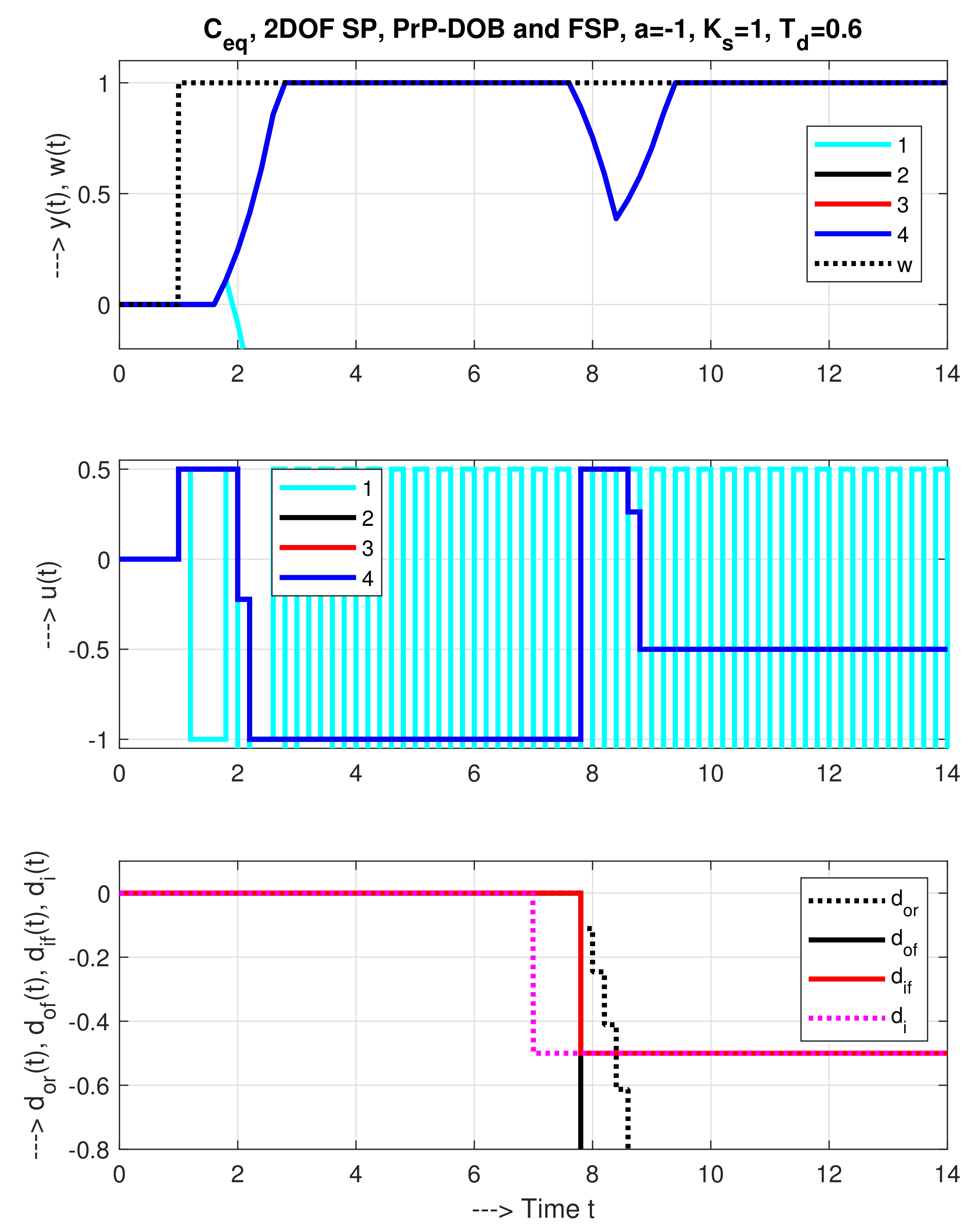
3.10. Example 3

Constrained (dead-beat) control with relatively long sampling period in Figure 11 enables to demonstrate in details some of the key characteristic properties of 2-DoF SP, FSP, of the equivalent controller $C_{eq}$ and of the PrP-DOB control. It again deals with the nominal model parameters ${\overline{K}}_s=K_s=1$, $\overline{a}=a=-1$, $T_d=0.6$ with four different situations:

• The equivalent controller $C_{eq}$ (Equation (56)) with a dead-beat tuning given by $T_s=0.2$, $T_c\to 0$, $K=0.2214$, $D=1.2214$, $D_c=0$, $K_p=5.5167$ (Equation (11)), $n=1$, $T_f\to 0$, $D_f=0$ and $\beta =7.7609$, which, in linear case, is fully equivalent to the FSP controller, yields under process input constraints $u\in [-1.1,0.5]$ fully unusable results (see Figure 11, response 1).
• In this respect, it may seem to be more suitable to apply the 2-DoF SP with dead-beat performance (Figure 11, response 2), using the same parameters. However, due to diverging reconstructed disturbance and unstable plant mode, it will be taken out of service in a short time.
• While used with the same parameter as in Example 1 for $k_t=k+1,n=0$, the disturbance response of the PrP-DOB controller with a dead-beat tuning (without additional filtration) shows the same amplitude of the disturbance rejection as the 2-DoF SP with dead-beat performance (Figure 11, response 3). However, the closed-loop response is stable.
• In Figure 11, the responses of the FSP controller (curves 4), the 2-DoF SP and the PrP-DOB controller fully overlap. The advantage is that FSP and PrP-DOB responses are internally stable. The disadvantage of FSP is that there is no reconstructed disturbance signal available.

3.11. Summary 3

In terms of the constrained dead-beat performance, the 2-DoF SP, the FSP and the PrP-DOB control may seem to be equivalent. However, the 2-DoF SP is unstable, its disturbance signal is diverging and thus giving no useful information and also the FSP does not give any information about the acting disturbances. From the practical point of view, the problem is that, despite the large number of publications on the topic of FSP, an evaluation considering control constraints, although extremely important, to the best of our knowledge, has not yet been published. In fact, without such a study, the FSP cannot be compared to simpler solutions with $C_{eq}$.

In practice, it will be necessary to work with the smallest possible sampling periods, while ensuring a sufficiently high processing speed (whether it is the suppression of noise or uncertainty).

4. Illustrative Example—Temperature Control

As for the illustration of the discussed controllers by real-time control, we do not know of an available unstable system with dominant first-order dynamics, which would allow safe experimentation in a laboratory environment. The unstable robotic arm used in the article [16] rather represents a system with unstable second-order dynamics that, in general, requires at least two pulses in the control signal course (corresponding to acceleration and braking), which should be respected in evaluating its dynamics (see, e.g., [10]). We will return to it when designing the corresponding controllers. With regard to the absence of suitable unstable processes with dominant first-order dynamics, we decided to illustrate at least the use of a simplified design of controllers based on the integrating models approximating a stable higher-order process.

For illustrating the controllers proposed, temperature control of an Arduino-based laboratory plant TOM1A [70,71,72] will be considered. Its heat channel consists of a 5 W bulb representing a heat source, a cooling fan used to generate disturbances, and a temperature sensor. Although it may be considered as a typically stable system, the marginally stable integrating models will be used here, as an DTC-based alternative to ADRC [24,39,40] and MFC [38], simplifying the plant modelling and controller design, and significantly shortening the plant model identification.

4.1. Loop Dynamics Modelling

Already in early works [19,20], the selection of the nominal model of the controlled system, based on two types of linear models (one created by the approximation of controlled dynamics by “ultra local” IPDT models and the other by “local” FOTD ones) was considered as one of the basic design steps. As other authors later confirmed [44], the basic model selection criterion should be its simplicity. So, although the controlled system is physically characterized by at least two modes of heat dissipation, one fast (radiation) and the other one slow (convection), the choice of models remains quite limited to FOTD and IPDT ones, representing just a single mode of the heat transfer. Given that this is a stable process, the approximation by the first-order model, and the rigorous evaluation of the achieved transients, do not pose any problems with regard to the permissible courses of the control signal variable.

Thereby, for the mentioned laboratory plant, the identification results from the previous papers [70,71] yield

$$K_{sm}=0.01;a_m=0.05{\mathrm{s}}^{-1};T_{dm}=0.3\mathrm{s};T_s=0.02\mathrm{s}$$

(57)

The identified plant dead time covers delay of the faster heat transfer by radiation, contribution of several possible shorter time delays and transport delay due to information processing and control signal calculation. Parameter $a_m$ corresponds to a plant time constant $T_{1m}=1/a_m\approx 20$ s, or it is chosen as $a_m=0$ (for IPDT model). The mode of slow heat conduction associated with heating the device body with a longer time constant in the range of 20 min is neglected. As a consequence of the simplified model, the results of the experiments will largely depend on whether they were obtained using a cold or already heated system. At the same time, they will also depend on the ambient temperature, which may change, especially during longer experiments (information recorded for each experiments includes both the board and the ambient temperatures). In such circumstances, the definition of a nominal system dynamics, representing frequently the cornerstone of robustness analysis, becomes questionable. Rather, it would make sense to define the interval for each considered model parameter, together with the ambient temperature value (if changed over a wider range). It should be noted here that, given the high degree of simplification, the use of both models can be considered as a robustness test for both types of controllers.

While in the simplest case the use of IPDT and FOTD models appears to differ only in the value of a single parameter $a_m$, it has a huge impact on the necessary identification experiment procedure. Obtaining a complete step-response for the FOTD model identification requires a several-hour experiment, in which the effect of variable outer (environment) disturbances must be excluded. However, to obtain a comparable IPDT model, an experiment lasting a few seconds is sufficient. In such a case, however, it is also necessary to take into account the differences in the parameters $K_{sm}$.

The situation is also complicated by a relatively high level of measurement noise. In order to achieve the best possible filtration, it is necessary to work with the smallest possible sampling period. With regard to the need for filtration in the following, we are using the design of PrP-DOB controller based on $k_t=k+2$.

4.2. Experiment Organization

The system output has been firstly brought to the temperature $w_0=31{}^{\circ }$C with the fan input set to $u_{fan}=5$ (see Figure 12). Then, a reference setpoint step change to $w_1=37{}^{\circ }$C has been applied at $t=50$ s. By increasing the fan input to $u_{fan}=15$, a disturbance step has been produced at $t=150$ s. Each measurement cycle finished with a cooling period with switched off bulb and fan set to $u_{fan}=100$ for the period of 100 s.

4.3. Performance Measures Used

When publishing the first critique of the traditional SP, concerning the unnecessary, or even harmful, inclusion of I-action in the primary feedforward loop, we thoroughly tested all claims with a number of simulations and real-time control experiments using nonlinear optical and thermal systems [63,64,65,66,67]. With regard to the possibility of immediate evaluation, we preferred time-domain performance measures (as used, for example, in [9]), namely the Integral of absolute error (IAE) of the output variable

$$IAE={\int }_0^{\infty }\left|e\left(t\right)\right|dt;e=w-y$$

(58)

and the Total Variation (TV) of the control signal

$$TVu\left(u\right)=\sum _i\left|u_{i+1}-u_i\right|$$

(59)

The Integral of Absolute Error (IAE) represents a quantitative performance measure used typically for evaluating the speed of transients [73]. It may be applied to the reference setpoint ($IA{E}_s$) and the input disturbance ($IA{E}_i$) step responses. In order to demonstrate a balanced performance view, in this paper, the loop evaluation considers the simple combined value

$$IAE=IA{E}_s+IA{E}_i$$

(60)

Of course, by weighing the individual components as in [74], we could refine the evaluation, but with respect to a number of other possible parameters, we will try to keep the evaluation as simple as possible.

Skogestad introduced $TV$ as a measure of an excessive control effort. However, as explained in [75], as the main qualitative parameters of a control design it is frequently useful to consider shapes of the resulting transient responses both at the plant input and output [72]. Among them, deviations from monotony can be used as a quantifiable measure. Since for a monotonic transient of a setpoint step response resulting into a process output change between $y_0$ and $y_1$, the total output variation $TV$ equals to the net output change $|y_1-y_0|$, an output deviation from monotonicity (MO) may be quantified by an excess of the $TV$ measure from the minimum necessary value, denoted as $T{V}_0$ (excessive variation):

$$T{V}_0\left(y_s\right)=\sum _i\left|y_{i+1}-y_i\right|-\left|y_{\infty }-y_0\right|$$

(61)

For a single integrator plant, the input corresponding to a MO output is a one-pulse (1P) signal [74]. This is formed by two MO intervals. Thus, the transient between the initial and the final input values $u_0$ and $u_{\infty }$ must be separated by an extreme point $u_m\notin (u_0,u_{\infty })$ (or an interval at a saturation limit) and the twice applied deviation from monotonicity (Equation (61)) yields together

$$T{V}_1\left(u\right)=\sum _i\left|u_{i+1}-u_i\right|-\left|2u_m-u_{\infty }-u_0\right|.$$

(62)

At the plant output, similar 1P shapes, quantified by $T{V}_1\left(y_i\right)$, occur after step-like disturbances. A well-balanced controller tuning may again consider combined values at the output and input

$$TV\left(y\right)=T{V}_0\left(y_s\right)+T{V}_1\left(y_i\right);TV\left(u\right)=T{V}_1\left(u_s\right)+T{V}_1\left(u_i\right);$$

(63)

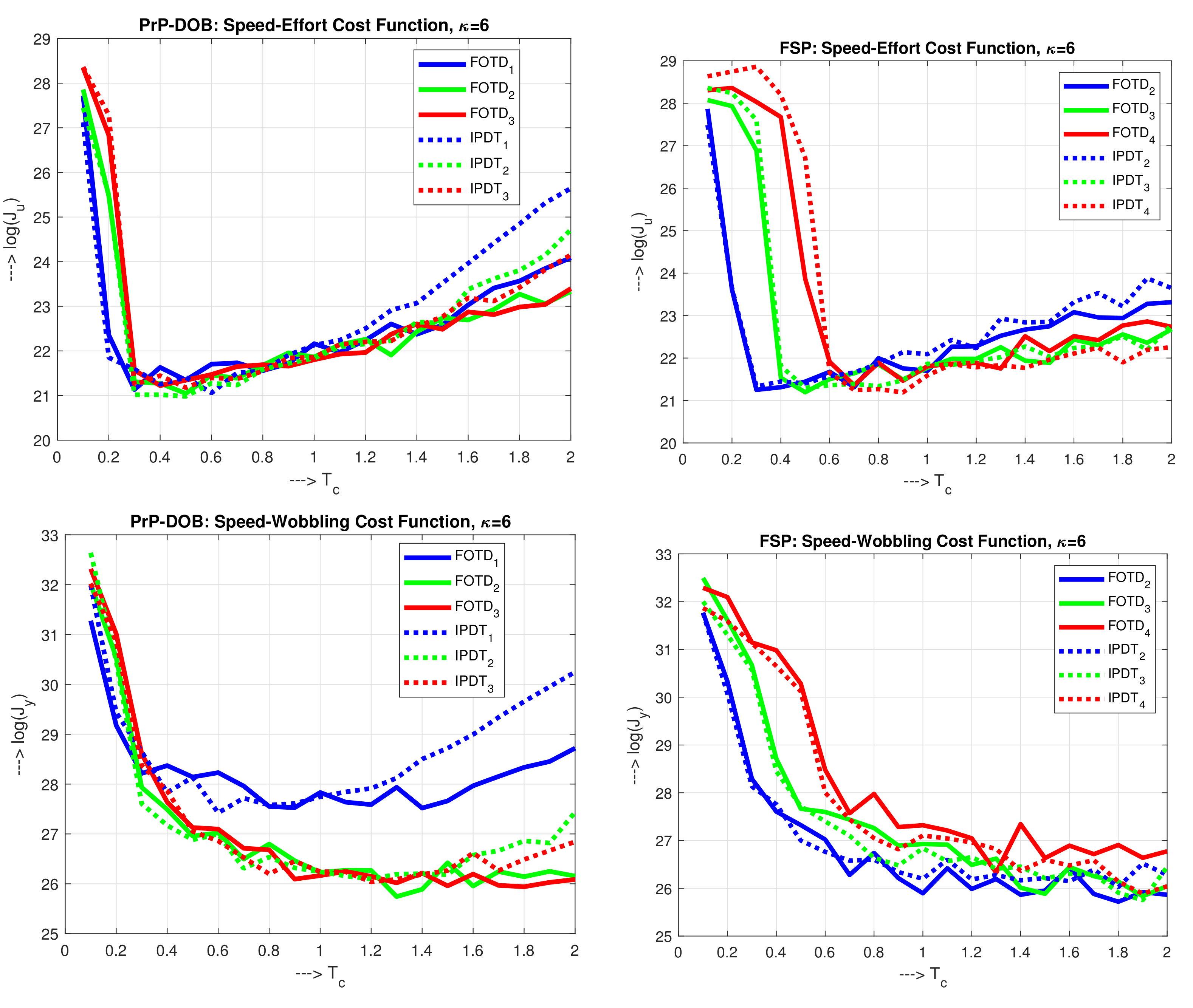
A “holistic” view (considering both the speed and shapes of responses) may be defined by the speed-effort (SE) cost function

$$J\left(u\right)=IA{E}^{\kappa }TV\left(u\right)$$

(64)

and or the speed-wobbling (SW) cost function

$$J\left(y\right)=IA{E}^{\kappa }TV\left(y\right)$$

(65)

with the parameter $\kappa$ representing the weight of $IAE$ (speed of control) in the evaluation. Besides speed of control, the SE cost function (64) focuses on smooth control signal and SW (Equation (65)) focuses on reduced output wobbling.

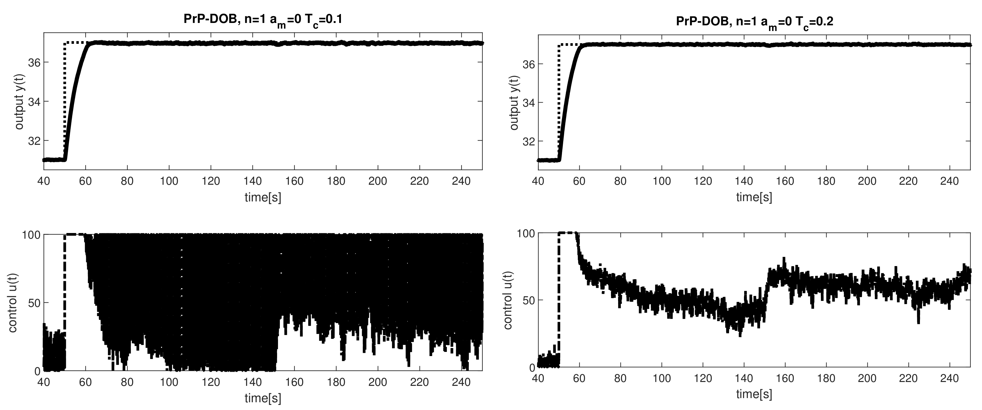
4.4. Application of the PrP-DOB Control

The first set of experiments has been carried out by PrP-DOB control structure, employing the output and disturbance reconstruction using three low pass filters ($n=1,2,3$), applied according to Figure 1. They have been tuned by the single tuning parameter $T_c\in [0.1,2]$ s, whereby the filter pole $\lambda =-n/T_c$ is chosen to yield a constant average residence time [61]$T_c=n/\left|\lambda \right|$ of the filter.

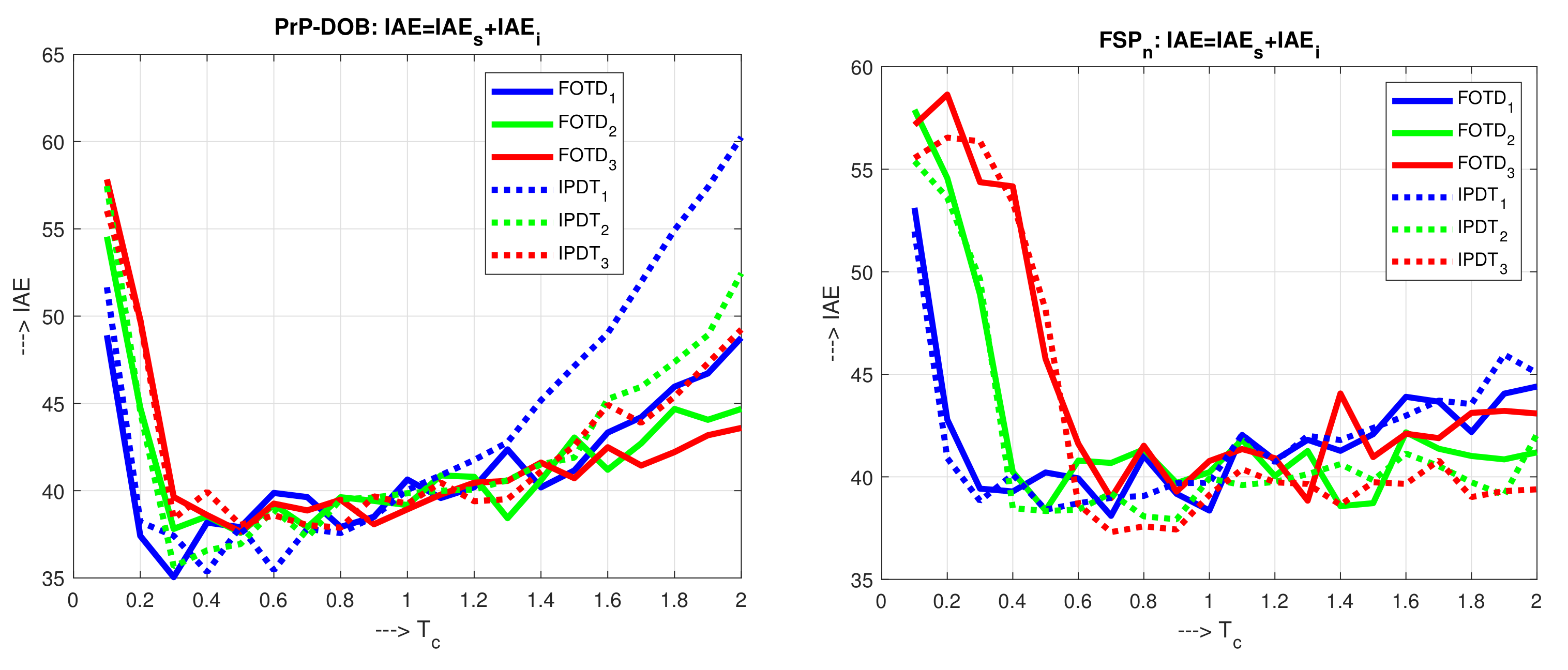
For the shortest $T_c$ values, the $IAE$ values are high due to the noisy overload plant input and output signals. By increasing $T_c$, the noise impact rapidly decreases (Figure 13). Despite the limitation of the control signal, there was no permanent control deviation at the output as discussed in [76]. Increase of $IAE$ at higher $T_c$ values appears due to slow down transients. However, the increase is not so high when increasing n. For larger $T_c$, the optimum $IAE$ values do not significantly depend on the type of model used. When applying larger $T_c$ values, $IAE$ increases more rapidly for IPDT models and for lower n (Figure 14 left).

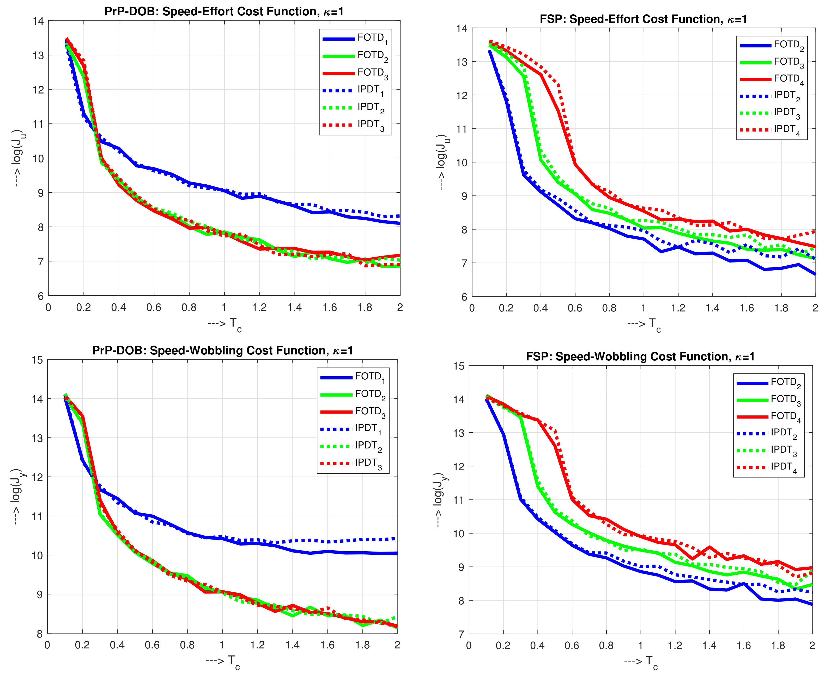
By using the “holistic” cost functions (64) and (65) considering with the weighting $\kappa =1$ both speed of the control and the shapes of transients (Figure 15 left), the achieved performance remains nearly the same for both considered models ($a_m=0$ and $a_m\ne 0$). This result again suggests that the controller is not sensitive to the accuracy of the determination of parameter $a_m$ and (similarly as in ADRC) it is enough to use simpler integrating models.

By using higher-order filters, performance may be significantly improved for longer $T_c$ (the considered cost function is displayed in a logarithmic scale). In the case of speed-wobbling cost function (Figure 15 left below), for $n=1$, the performance improvement by increasing $T_c$ is strongly limited for both models.

With increased control error weighting $\kappa =6$ in the holistic cost functions (64) and (65) (Figure 16 left), the possibilities of improving performance by increasing $T_c$ will be limited—for SE cost function significantly more than for SW one. The different positions of the optimal points with the minimum values of the individual cost functions illustrate why the optimal setting of the controllers cannot be crammed into a single optimal relationship, or rule, covering all possible requirements of practice. However, it turns out that in a large number of situations, it will be possible to suffice with the choice of IPDT model and $n=2$ regarding the filter degree.

4.5. Application of the FSP Controller

For the shortest $T_c$, the corresponding $IAE$ values (Figure 14 right) are high due to the noise at the process output. By increasing $T_c$, the $IAE$ values decrease to a minimum, from which they grow again due to slowing down the process. Surprisingly, the optimum $IAE$ values correspond to a simpler IPDT model with the highest filter order n. The minimum achievable $IAE$ values are slightly higher than with the PrP-DOB controller.

Unlike the PrP-DOB controller, the increased n increases cost functions (64) and (65) (Figure 15 right). However, it should be noted that for FSP we worked with low-pass filter degrees 2,3,4, while in the first method it was the degree one lower. With a similar choice of FSP degrees from 1 [72], the worst effect of noise for the minimum value of n was shown there as well.

As with the PrP-DOB controller, the combined functions decrease with increasing $T_c$. Effects of an increased control error weighting achieved with $k=6$ in holistic cost functions (64) and (65) (Figure 16 right) are similar to those with PrP-DOB control, just the particular minima are shifted to higher $T_c$ values.

4.6. Summary 4

Real-time experiments on a thermal plant confirmed the equivalence of the compared PrP-DOB and FSP controllers in terms of the transients performance. Although the characteristics of the selected performance indicators depending on $T_c$ have different shapes, the achieved optimal values are fully comparable.

At the same time, the results show that by not considering possibilities of the simplified process modelling given by the use of IPDT approximations, the works from the DTC area (as, e.g., [14,16]) neglect possibilities of a significant design simplification offered by ADRC and MFC control. Although, as can be verified by simulation with web applications, in unstable systems, the quality of transients based on design using integral models will decrease with a $T_d$ value much faster than in stable systems (similarly as in PID control [12]).

5. Discussion of the Results

The above results obtained by both simulation and real-time control should be reason enough to rewrite or add to some of the listed references in [14], which represent a whole body of work on FSP. Part of the problems has already been explained in the article [16]. However, since the number of papers written on FSP and based on a primary loop with a PI control is really high, see, e.g., [47,48,49,51,52,53,54,55], whereas it was not sufficiently explained why the conceptual schemes, implementation and equivalent controller differ and what are the impacts on the control task, it may take longer to correct the understanding of SP, FSP and other alternatives in DTC design. Because many explanations are still lacking in the current literature, we believe that this work helps uncover some hidden secrets.

On the other hand, problems with the control based on integrating models seem to have contributed to the fact that users of structures inspired by Smith’s predictor did not notice possible simplifications brought by their use into identification and control and which are already for long time in the focus of attention in the field of ADRC.

In our future work, we will focus more on the limitations of SP. It is not widely known that SP cannot be applied to unstable systems with larger delays because such a delay makes the whole control system unstable, but the structure could be used after introducing a stabilizing controller complemented by a disturbance reference model [18]. Or that SP becomes redundant for stable systems with larger delays and it is easier to modify the solution based on the Reswick solution [10,77]. Another direction of our research will deal with the possibility of using additional information based on the analysis of the reconstructed disturbance provided by the PrP-DOB controller.

6. Conclusions

The article has shown that several facts important for the control of simple first-order time-delayed systems are still unknown to the broad control community. Insufficiently known or clearly explained aspects then result in insufficient use of the advantages of already existing solutions and their generalization for more complex tasks. Indeed, the fact that the reader is not provided with all the information that would allow him to understand the DTCs at hand is the central aspect of the problem considered and constitutes obstacles to the further development of time-delayed systems control. To make progress, it is important to place DTCs in the broader context of control methods, combined with a clarification of the common relationships and differences. In a series of articles focused on the DTCs for stable, unstable and integrating models, we have shown that limiting this issue to FSP is very restrictive, even misleading. We have shown several new possibilities of designing alternative solutions while maintaining the full functionality of the original SP, i.e., also the signal of the reconstructed disturbance. Two different recently published designs of DTCs with stabilizing controllers have been extended with a third one based on the ESO design and extended by polynomial interpretation, providing an input disturbance signal and an undelayed plant output, which allow the stabilizing controller to increase the speed of transients. We hope that such a responsible approach to all design issues allows to find a response to articles such as “Grimholt and Skogestad: Should we forget the Smith Predictor?” from the PID2018 conference [11]. We see the starting point for improving the situation in this area as taking note of all the solutions that exist in this area, not just some of them, calling them by their proper names, respecting the essential points of their design, and considering all the important aspects in their implementation.