Dynamic Graph Learning for Session-Based Recommendation

Abstract

Session-based recommendation (SBRS) aims to make recommendations for users merely based on the ongoing session. Existing GNN-based methods achieve satisfactory performance by exploiting the pair-wise item transition pattern; however, they ignore the temporal evolution of the session graphs over different time-steps. Moreover, the widely applied cross-entropy loss with softmax in SBRS faces the serious overfitting problem. To deal with the above issues, we propose dynamic graph learning for session-based recommendation (DGL-SR). Specifically, we design a dynamic graph neural network (DGNN) to simultaneously take the graph structural information and the temporal dynamics into consideration for learning the dynamic item representations. Moreover, we propose a corrective margin softmax (CMS) to prevent overfitting in the model optimization by correcting the gradient of the negative samples. Comprehensive experiments are conducted on two benchmark datasets, that is, Diginetica and Gowalla, and the experimental results show the superiority of DGL-SR over the state-of-the-art baselines in terms of Recall@20 and MRR@20, especially on hitting the target item in the recommendation list.

1. Introduction

Recommender systems can help provide users with personalized information according to their preference reflected in the historical interactions [1,2,3], which are widely applied in e-commerce websites, web search, and so forth [4,5]. However, in some scenarios where only the user’s recent interactions are available, the general recommenders are not applicable, since the user’s inherent preference is unknown [6]. Thus, session-based recommendation (SBRS) is proposed, which aims to detect the user intent from the limited interacted items in the current session and make recommendations, where the session is defined as the user’s actions within a period of time (e.g., 24 h) [6,7].

Existing methods for SBRS mainly focus on the sequential signal [6,7,8] and the pair-wise transitions between items [9,10,11], as well as the item importance [12,13,14]. For example, traditional methods, such as Markov chains (MC) and neural models like recurrent neural networks (RNNs) can be utilized to model the sequential information between items in the current session [6,15,16]. Moreover, graph neural networks (GNNs) are recently applied to take the complex pair-wise item transition relations into consideration [9,17,18], such as adopting the gated graph neural network (GGNN) [19] to propagate the information flow between items. In addition, the attention mechanism is widely applied to focus on user’s main intent by distinguishing different items according their corresponding importances, which can be utilized individually [12,13,20] or together with the sequential models [7,8] and GNN-based methods [9,17].

Though considerable performance has been achieved, there still remains some limitations. First, it has been proven by multiple works [9,10] that RNN- or attention-based methods fail to consider the complex item transitions, leading to unsatisfying performance [9,10]. Though the GNN-based methods alleviate the problem [9,17,21], they adopt the mechanism that transforms the snapshots of the session at different timestamps into individual graphs to model the static structural information, without taking the temporal evolution of the item transition relations into consideration. On the other hand, the state-of-the-art methods for SBRS all adopt the cross-entropy loss with softmax for optimizing the model parameters, where all the items (excluding the target item) are regarded as the negative samples and treated equally for comparison during training. However, for the negative items with low prediction scores, a continued decrease of their scores may cause model overfitting and loss of generalization ability. Moreover, for the top-ranked negative items, the cross-entropy with softmax cannot provide a sufficiently large gradient for lowering their scores [16,22], limiting the convergence speed of the model.

To solve the above problems, we propose the dynamic graph learning for session-based recommendation (DGL-SR). Specifically, given an ongoing session, we transform the session into a dynamic graph which can simultaneously consider the structural information through the graph attention network (GAT) and the temporal evolution of the graph structures over different time-steps by the temporal attention. Then, we generate the dynamic user preference, which is utilized to produce the prediction scores on all candidate items. Finally, we design a corrective margin softmax (CMS) to correct the gradients of the negative items for preventing overfitting and achieving effective model optimization.

We conduct comprehensive experiments on two publicly available datasets, that is, Diginetica and Gowalla, and the experimental results show that DGL-SR can achieve a state-of-the-art performance in terms of Recall@20 and MRR@20 on the session-based recommendation task.

We summarize the main contributions in this paper as follows:

• To the best of our knowledge, we are the first to consider the dynamic temporal evolution of the item transitions in the ongoing session for a session-based recommendation;
• We propose a dynamic graph neural network (DGNN) for the item representation learning, which can simultaneously take the structural information and the temporal dynamics into consideration;
• We design a corrective margin softmax (CMS) to correct the gradients of the negative items for simultaneously achieving effective model optimization and avoiding overfitting;
• Extensive experiments conducted on two public datasets demonstrate that DGL-SR can outperform the baselines in terms of Recall@20 and MRR@20.

2. Related Work

The existing methods for SBRS mainly concentrate on the sequential signal in the session or the pair-wise item transitions between items, which correspond to the sequential methods and the GNN-based models, respectively. In this section, we first review the related work about the sequential methods in Section 2.1, and then provide more detail of the GNN-based models in Section 2.2.

2.1. Sequential Methods

For the sequential models, traditional methods like Markov Chains are widely applied to capture the sequential dependencies between adjacent items. For example, Shani et al. [23] introduced the Markov decision processes (MDPs) into recommender systems by regarding the the recommendation generation as a sequential optimization problem, and Rendle et al. [15] combined the Markov chains (MC) with the matrix factorization (MF) to capture the user’s dynamic and inherent preferences, respectively. Moreover, deep learning methods, such as RNNs, are also widely utilized to process the item sequence in the ongoing session. For instance, Hidasi et al. [6] first utilized the gated recurrent units (GRUs) to model the sequential signal in the current session; then Hidasi and Karatzoglou [16] further improved the loss functions for SBRS to solve the gradient vanishing problems. Moreover, some following studies have aimed to emphasize the user’s main intent [7], incorporate collaborative information from the neighbor sessions [8,24,25], explore the repeated consumption of user behaviors [26], and so forth to improve the recommendation accuracy.

However, the sequential methods simply regard the session as an item sequence, failing to take the complex transition pattern between items into consideration [9,10].

2.2. GNN-Based Methods

In order to take the complicated transition relationship between items into consideration, GNNs are introduced into SBRS [9,10,27]. For example, Wu et al. [9] first proposed to utilize the graph structure to process the ongoing session by adopting the gated graph neural networks (GGNNs) to generate the item representations. Then, Qiu et al. [10] designed a weighted GAT which can attentively compute the information flow between items in the information propagation, and aggregate the item representations as the user’s preference by a Readout function [28]. Moreover, Xu et al. [29] introduced the self-attention mechanism into the GNNs, and Pan et al. [17] designed a star graph neural network (SGNN) to explore the long-range dependencies between items in the session. Furthermore, Chen and Wong [21] focused on handling the information loss in GNNs for SBRS by preserving the edge order and adding shortcut connections. In addition, Wang et al. [11] proposed to enhance the representation learning of items in the current session by the global-level item transitions.

However, the existing GNN methods all transform the session into static graphs, without considering the temporal dynamic evolution of the graph structures over various time-steps. Moreover, the overfitting problem in GNNs for SBRS seriously limits the recommendation performance [9,17].

3. Approach

In this section, we first formulate the definition of the session-based recommendation task. Then, we describe our proposed dynamic graph learning for session-based recommendation (DGL-SR) in detail, which is constituted of three main components, that is, the dynamic item representation learning, the user preference generation and prediction, and the corrective model optimization.

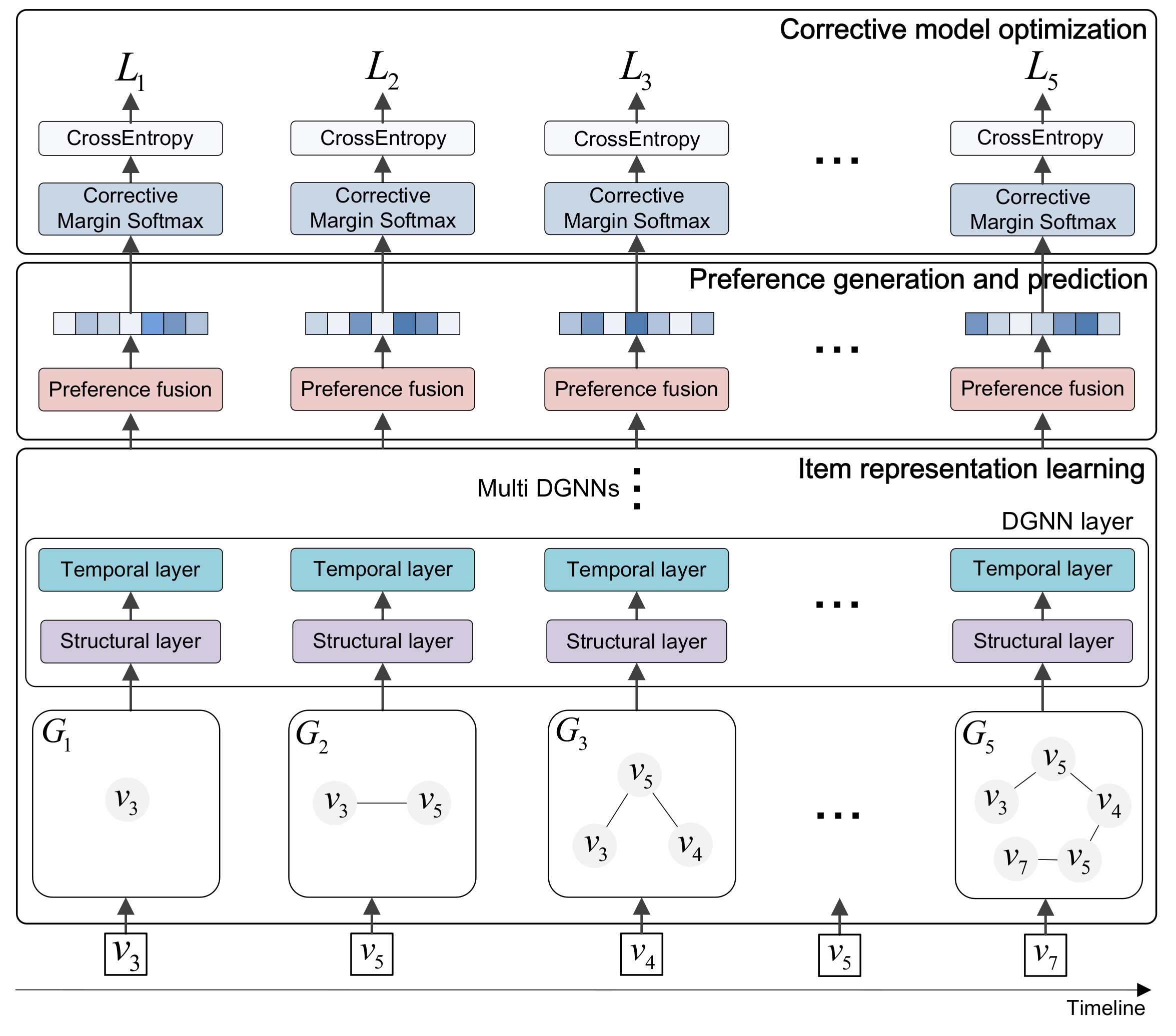
The framework of the proposed DGL-SR is plotted in Figure 1.

Given an ongoing session, we first construct a dynamic graph which contains the graphs transformed from the session snapshots at different timestamps. Then, we learn the dynamic item representations through the dynamic graph neural network (DGNN). After that, we generate the hybrid user preference, which is utilized to make predictions on all candidate items. Finally, we correct the gradients of the negative items using the corrective margin softmax (CMS) to achieve effective model optimization.

We assume the item set is $V=\{v_1,v_2,\dots ,v_{\left|V\right|}\}$, where $v_i$ indicates an item and $\left|V\right|$ is the number of all items. Giving an ongoing session denoted as $S=\{v_1,v_2,\dots ,v_n\}$, the aim of a session-based recommendation is to predict the item that the user will interact with at the next timestamp, that is, $v_{n+1}$. Specifically, we input the session S into DGL-SR to output the prediction scores on all candidate items, then the items ranked at the top K positions will be recommended to the user.

The main abbreviations used in this paper are listed in

Table 1. Main abbreviations used in this paper.

Abbreviation	Explanation
SBRS	Session-based Recommender Systems
DGL-SR	Dynamic Graph Nueral Networks for Session-based Recommendation
DGNN	Dynamic Graph Nueral Networks
CMS	Corrective Margin Softmax
MC	Markov Chains
RNNs	Recurrent Neural Networks
GNNs	Graph Neural Networks
GGNNs	Gated Graph Neural Networks
GATs	Graph Attention Networks
MF	Matrix Factorization
GRUs	Gated Recurrent Units
SGNNs	Star Graph Neural Networks
BPTT	Back-Propagation Through Time

.

3.1. Dynamic Item Representation Learning

Given a session inputted to DGL-SR, we first generate the dynamic representation of the contained items using the dynamic graph neural network (DGNN), which consists of three components, that is, the dynamic graph construction, the structural layer, and the temporal layer.

3.1.1. Dynamic Graph Construction

Given session $S=\{v_1,v_2,\dots ,v_n\}$, we first generate the snapshots of the session and their corresponding target items at different timestamps as $({\tilde{S}}_1,v_2),({\tilde{S}}_2,v_3),\dots ,({\tilde{S}}_{n-1},v_n)$ where ${\tilde{S}}_t=\{v_1,v_2,\dots ,v_t\}$. This is similar to the data augmentation method widely applied in SBRS [9,17]. However, different from the existing methods which shuffle the augmented samples and utilize them for training individually, in our DGNN we capture the temporal evolution of the session graphs over multi-time steps. Specifically, we construct a dynamic graph denoted as $G=\{G_1,G_2,\dots ,G_{n-1}\}$, where $G_t$ is the session graph constructed from the item sequence ${\tilde{S}}_t$, which includes the items that the user has interacted with till the t-th timestamp. Here, $G_t=\{V_t,E_t\}$, where $V_t$ is the items in ${\tilde{S}}_t$, that is, $V_t=\{v_1,v_2,\dots ,v_t\}$. Additionally, each edge $(v_i,v_j)\in E_t$ indicates that the items $v_i$ and $v_j$ are adjacently clicked in the item sequence ${\tilde{S}}_t$. Moreover, for the items without a self-connection, we add a self-loop to help propagate information from the item itself. In addition, note that for the items repeatedly interacted with, we learn different representations of the items for various timestamps, which can help generate dynamic item representations for accurate user preference generation, as stated in [29].

3.1.2. Structural Layer

After constructing the dynamic graph, we first utilize the structure layer to take the structural information into consideration to learn the representation of the items in session S over different time-steps. Specifically, as for the graph snapshot $G_t$, we update the item representations in $G_t$ using the graph attention network (GAT). Specifically, for an item $v_i$ where the neighbors of $v_i$ is $N\left(v_i\right)$, we propagate information from the neighbors $N\left(v_i\right)$ to update the item representation of $v_i$. First, we calculate the similarity of item $v_i$ with its neighbors to determine the importance of each neighbor using the self-attention mechanism:

$$e_{ij}=\frac{{\left({\tilde{\mathbf{W}}}_q{\mathbf{v}}_i\right)}^{\mathsf{T}}\left({\tilde{\mathbf{W}}}_k{\mathbf{v}}_j\right)}{\sqrt{d}},$$

(1)

where $v_j\in N\left(v_i\right)$ is a neighbor of $v_i$, and ${\mathbf{v}}_i,{\mathbf{v}}_j\in {\mathbb{R}}^d$ are the embeddings of item $v_i$ and $v_j$, respectively. ${\tilde{\mathbf{W}}}_q,{\tilde{\mathbf{W}}}_k\in {\mathbb{R}}^{d\times d}$ are the trainable parameters, and $\sqrt{d}$ is used to scale the attention scores.

Then, we normalize the generated scores using the softmax layer to obtain the importance score of each neighbor as follows:

$${\alpha }_{ij}=\mathrm{Softmax}\left(e_{ij}\right)=\frac{exp\left(e_{ij}\right)}{{\sum }_{v_k\in N\left(v_i\right)}exp\left(e_{ik}\right)}.$$

(2)

After that, we combine the representations of the neighbors of $v_i$ as the updated vector of item $v_i$ according to the generated importance scores:

$${\tilde{\mathbf{v}}}_i^t=\sigma \left(\sum _{v_j\in N\left(v_i\right)}{\alpha }_{ij}{\tilde{\mathbf{W}}}_v{\mathbf{v}}_j\right),$$

(3)

where ${\tilde{\mathbf{v}}}_i^t\in {\mathbb{R}}^d$ is the updated representation of item $v_i$ in $G_t$, and ${\tilde{\mathbf{W}}}_v\in {\mathbb{R}}^{d\times d}$ is the trainable parameters. Through the structural layer in DGNN, we can learn the structural representation of the items in each graph snapshot $G_t\in G$ by propagating information from the neighbors of each item.

3.1.3. Temporal Layer

To capture the temporal evolution of the session graphs over various time-steps, we propose to generate the representation with the temporal characteristics of each item using the temporal layer in DGNN. Specifically, for an item $v_i$ where the structural representations generated by the structural layer at different timestamps is $\{{\tilde{\mathbf{v}}}_i^1,{\tilde{\mathbf{v}}}_i^2,\dots ,{\tilde{\mathbf{v}}}_i^n\}$ (here, the superscript indicates the time index while the subscript denotes the item index. Moreover, note that items occurring several times in the session are denoted by different subscripts to distinguish them), we attentively combine the item vectors of $v_i$ over different time-steps to capture the evolution of the temporal characteristics of $v_i$.

To generate the temporal representation of item $v_i$ at the t-th timestamp, here we adopt the self-attention mechanism to assign different importance scores for the item vectors of $v_i$ at different timestamps, which can be denoted as follows:

$${\epsilon }_{t\tau }=\frac{{\left({\widehat{\mathbf{W}}}_q{\tilde{\mathbf{v}}}_i^t\right)}^{\mathsf{T}}\left({\widehat{\mathbf{W}}}_k{\tilde{\mathbf{v}}}_i^{\tau }\right)}{\sqrt{d}},$$

(4)

where ${\tilde{\mathbf{v}}}_i^t,{\tilde{\mathbf{v}}}_i^{\tau }\in {\mathbb{R}}^d$ are the representations of item $v_i$ at the t-th and $\tau$-th timestamps, respectively. ${\widehat{\mathbf{W}}}_q,{\widehat{\mathbf{W}}}_k\in {\mathbb{R}}^{d\times d}$ are the learnable parameters, and $\sqrt{d}$ is used for scaling the attention. Here, the vector of item $v_i$ at the current timestamp (i.e., the t-th timestamp) is deemed as the “query” to select information from the historical timestamps.

Considering that the item vectors after the t-th timestamp (i.e., $\tau >t$) are unavailable for updating the item vector of $v_i$ at the t-th timestamp, here we add a mask operation which can be denoted as follows:

$$m_{t\tau }=\left\{\begin{array}{cc}0,\hfill & \hfill \tau \le t\\ -\infty ,\hfill & \hfill \mathrm{otherwise}\end{array}\right.$$

(5)

Then we normalize the sum of the attention scores generated by Equation (4) and the mask matrix generated by Equation (5) as the importance scores, which can be noted as follows:

$$\begin{array}{cc}\hfill {\beta }_{t\tau }& =\mathrm{Softmax}\left({\epsilon }_{t\tau }^{\prime }\right),\hfill \\ \hfill {\epsilon }_{t\tau }^{\prime }& ={\epsilon }_{t\tau }+m_{t\tau }.\hfill \end{array}$$

(6)

After that, the representations of item $v_i$ over multi-time steps are attentively combined according to the importance scores as follows:

$${\widehat{\mathbf{v}}}_i^t=\sigma \left(\sum _{\tau =1}^n{\beta }_{t\tau }{\widehat{\mathbf{W}}}_v{\tilde{\mathbf{v}}}_i^{\tau }\right),$$

(7)

where ${\widehat{\mathbf{v}}}_i^t$ is the generated temporal representation of item $v_i$ at the t-th timestamp, and ${\widehat{\mathbf{W}}}_v\in {\mathbb{R}}^{d\times d}$ is the trainable parameters. Through the temporal layer in DGNN, we can capture the temporal evolution of the characteristics of items over different time-steps in G, and thus generate the dynamic item representations.

3.1.4. Multi-Layer DGNNs

Moreover, multi-layers of DGNNs can be stacked, where each DGNN layer contains a structural layer and a temporal layer. Specifically, for $G_t$, the l-layer DGNN can be formulated as:

$${\tilde{\mathbf{V}}}_l^t,{\widehat{\mathbf{V}}}_l^t=\mathrm{DGNN}({\tilde{\mathbf{V}}}_{l-1}^t,{\widehat{\mathbf{V}}}_{l-1}^t),$$

(8)

where ${\tilde{\mathbf{V}}}_l^t,{\widehat{\mathbf{V}}}_l^t$ are the respective structural and temporal representations of the items at the l-th layer of DGNNs in $G_t$.

After that, we concatenate the structural and temporal outputs of L layers of DGNNs as the final item representations as follows:

$${\overline{\mathbf{V}}}^t={\mathbf{W}}_1[{\tilde{\mathbf{V}}}_1^t;{\widehat{\mathbf{V}}}_1^t;{\tilde{\mathbf{V}}}_2^t;{\widehat{\mathbf{V}}}_2^t;\dots ;{\tilde{\mathbf{V}}}_L^t;{\widehat{\mathbf{V}}}_L^t],$$

(9)

where ${\overline{\mathbf{V}}}^t=({\overline{\mathbf{v}}}_1^t,{\overline{\mathbf{v}}}_2^t,\dots ,{\overline{\mathbf{v}}}_n^t)$ is the representations of the items at the t-th timestamp. Here, $[·]$ denotes the concatenation, L is the layer number of DGNNs, and ${\mathbf{W}}_1\in {\mathbb{R}}^{d\times 2Ld}$ is the trainable parameters.

3.2. User Preference Generation and Prediction

After obtaining the item representations at the t-th timestamp, that is, the item vectors in $G_t$ which can be denoted as $({\overline{\mathbf{v}}}_1^t,{\overline{\mathbf{v}}}_2^t,\dots ,{\overline{\mathbf{v}}}_n^t)$, we generate the hybrid preference at the t-th timestamp. Specifically, we obtain the user’s preference by combining the recent interest and the long-term preference in the ongoing session. Considering that the latest clicked item can represent the user’s instant intent, here we directly adopt the vector of the last item as the recent interest, that is, ${\mathbf{z}}_r^t={\overline{\mathbf{v}}}_t^t$, where ${\mathbf{z}}_r^t\in {\mathbb{R}}^d$.

On the other hand, since the interacted historical items have various priorities, we utilize an attention mechanism to determine the weights for combining the historical item vectors as the user’s long-term preference, which can be denoted as:

$$\begin{array}{cc}\hfill {\mathbf{z}}_l^t& =\sum _{i=1}^t{\gamma }_i{\overline{\mathbf{v}}}_i^t,\hfill \\ \hfill {\gamma }_i& =\mathrm{Softmax}\left({\omega }_i\right),\hfill \\ \hfill {\omega }_i& ={\mathbf{W}}_2\sigma ({\mathbf{W}}_3{\overline{\mathbf{v}}}_i^t+{\mathbf{W}}_4{\mathbf{z}}_r^t+\mathbf{b}),\hfill \end{array}$$

(10)

where ${\mathbf{z}}_l^t\in {\mathbb{R}}^d$ is the generated long-term preference at the t-th timestamp, ${\omega }_i$ and ${\gamma }_i$ are the importance scores of item $v_i$ before and after normalization, respectively, and ${\mathbf{W}}_2\in {\mathbb{R}}^d,{\mathbf{W}}_3,{\mathbf{W}}_4\in {\mathbb{R}}^{d\times d},\mathbf{b}\in {\mathbb{R}}^d$ are learnable parameters.

Then, we generate the dynamic hybrid user preference by taking both the long-term and recent interests into consideration, as follows:

$${\mathbf{z}}_h^t={\mathbf{W}}_5[{\mathbf{z}}_l^t;{\mathbf{z}}_r^t],$$

(11)

where ${\mathbf{z}}_h^t\in {\mathbb{R}}^d$ is the final generated user preference at the t-th timestamp, and ${\mathbf{W}}_5\in {\mathbb{R}}^{d\times 2d}$ is the trainable parameters.

After that, we can make predictions by computing a probability distribution of the candidate items to be clicked at the next timestamp through the multiplication operation between the user preference and the embeddings of each item in V:

$${\widehat{\mathbf{y}}}_i^t={\left|\right|{\mathbf{z}}_h^t\left|\right|}^{\mathsf{T}}\left|\right|{\mathbf{v}}_i\left|\right|,$$

(12)

where ${\widehat{\mathbf{y}}}^t=\{{\widehat{\mathbf{y}}}_1^t,{\widehat{\mathbf{y}}}_2^t,\dots ,{\widehat{\mathbf{y}}}_{\left|V\right|}^t\}$ are the prediction scores on all items at the t-timestamp, and $\left|\right|·\left|\right|$ denotes the L2 normalization operation.

3.3. Corrective Model Optimization

In this section, we first describe our proposed corrective margin softmax (CMS) in detail in Section 3.3.1, and then provide detailed theoretical analysis to explain why the CMS can effectively address the overfitting problem in the session-based recommendation in Section 3.3.2.

3.3.1. Corrective Margin Softmax

After obtaining the prediction scores, the existing methods for SBRS all adopt the cross-entropy with softmax to train the model, which we argue faces a serious overfitting problem, limiting the generalization ability of the model. Thus, we propose the corrective margin softmax (CMS) to correct the gradients of the negative items for simultaneously preventing overfitting and achieving effective model optimization.

Specifically, we first calculate the difference of the prediction scores between each negative item and the target item as the correction values, as follows:

$${\Delta }_i^t=\sigma ({\widehat{\mathbf{y}}}_i^t-{\widehat{\mathbf{y}}}_{+}^t)-\delta ,\forall i\in V\backslash v_{+}^t,$$

(13)

where ${\widehat{\mathbf{y}}}_i^t$ and ${\widehat{\mathbf{y}}}_{+}^t$ are the prediction scores of the negative item $v_i$ and the target item $v_{+}^t$ at the t-th timestamp, respectively, and $\sigma$ denotes the sigmoid function. $V\backslash v_{+}^t$ indicates the negative items, that is, all the items except the target item in V, where “\” indicates the set subtraction operation. $\delta$ is a hyper-parameter controlling the boundary of adjusting the gradients, which we set as 0.5, that is, the value of $\sigma ({\widehat{\mathbf{y}}}_{+}^t-{\widehat{\mathbf{y}}}_{+}^t)$.

Next, we combine the original prediction scores of the negative items with their corresponding correction values as the final scores of them:

$${\tilde{\mathbf{y}}}_i^t={\widehat{\mathbf{y}}}_i^t+\alpha {\Delta }_i^t,\forall i\in V\backslash v_{+}^t,$$

(14)

where $\alpha$ is a parameter for controlling the correction intensity. Moreover, as for the target item, we directly take the prediction score as the corrective score, that is, no correction is conducted on the target item, which can be denoted as ${\tilde{\mathbf{y}}}_{+}^t={\widehat{\mathbf{y}}}_{+}^t$.

After that, we normalize the scores on all items using the softmax layer with a temperature $\lambda$ as follows:

$${\overline{\mathbf{y}}}_i^t=\mathrm{Softmax}\left(\lambda {\tilde{\mathbf{y}}}_i^t\right),$$

(15)

where $\lambda$ is utilized for preventing the nonconvergence problem [30].

Finally, we adopt the cross-entropy as the optimization objective:

$$L=\sum _{t=1}^n{L}^t=-\sum _{t=1}^n\sum _{i=1}^{\left|V\right|}{\mathbf{y}}_i^{t}log\left({\overline{\mathbf{y}}}_i^t\right),$$

(16)

where ${\mathbf{y}}^t$ denotes the one-hot encoding vector of the ground truth at the t-timestamp, and ${\overline{\mathbf{y}}}^t$ is the corresponding corrective scores generated by Equation (15). In addition, the back-propagation through time (BPTT) algorithm [31] is utilized to train DGL-SR. In general, the trainable parameters in our proposed DGL-SR consist of three main parts, that is, the item embeddings $\mathbf{V}\in {\mathbb{R}}^{\left|V\right|\times d}$, the learnable weights in DGNNs including ${\tilde{\mathbf{W}}}_q,{\tilde{\mathbf{W}}}_k,{\tilde{\mathbf{W}}}_v,{\widehat{\mathbf{W}}}_q,{\widehat{\mathbf{W}}}_k,{\widehat{\mathbf{W}}}_v,{\mathbf{W}}_1\in {\mathbb{R}}^{d\times d}$, and the learnable weights for user preference generation, including ${\mathbf{W}}_2,{\mathbf{W}}_3,{\mathbf{W}}_4,{\mathbf{W}}_5\in {\mathbb{R}}^{d\times d}$.

3.3.2. Theoretical Analysis

In this section, we provide a detailed theoretical analysis to explain why the proposed corrective margin softmax (CMS) can simultaneously solve the overfitting problem and achieve effective model optimization. Specifically, assuming the correction value we add on, the original prediction score of the negative item $v_i$ is $m_i$. Taking the t-timestamp as an example, the gradient of the loss at the t-th timestamp, that is, $L^t$ w.r.t, the negative prediction score ${\widehat{\mathbf{y}}}_i^t$ can be formulated as:

$$\frac{\partial L^t}{\partial {\widehat{\mathbf{y}}}_i^t}=1-\frac{exp\left({\widehat{\mathbf{y}}}_{+}^t\right)+{\sum }_{v_j\in V\backslash v_{+}^t,j\ne i}exp({\widehat{\mathbf{y}}}_j^t+m_j)}{exp\left({\widehat{\mathbf{y}}}_{+}^t\right)+{\sum }_{v_j\in V\backslash v_{+}^t,j\ne i}exp({\widehat{\mathbf{y}}}_j^t+m_j)+exp({\widehat{\mathbf{y}}}_i^t+m_i)},$$

(17)

where we can see that comparing to the original softmax, that is, $m_i$ is 0, a positive $m_i$ can increase the gradient of negative item $v_i$, thus the score can be decreased faster. On the contrary, a negative value of $m_i$ will slow down the decreasing speed of ${\widehat{\mathbf{y}}}_i^t$.

Then we discuss the situations for the negative items with larger and smaller prediction scores than the target item $v_{+}^t$ separately:

• First, for the negative items with smaller prediction scores than $v_{+}^t$, from Equation (13) we can see that the correction value $m_i$ is negative, then the decreasing of the prediction score will slow down to avoid overfitting. This could be explained by the fact that there are merely positive interactions in SBRS, and we cannot conclude whether the user likes the left items $V\backslash v_{+}^t$ or not; thus, pushing the prediction scores of $V\backslash v_{+}^t$ too small in the training set will make them completely unable to be recommended in the validation and test sets. By slowing down the decreasing of the scores of items with low prediction scores, the CMS can avoid the above issue to prevent the overfitting problem.
• On the other hand, for the negative items with larger prediction scores than the target item $v_{+}^t$, the correction value $m_i$ is greater than 0; thus, our proposed CMS can provide a larger gradient than the original softmax to accelerate the decreasing of the negative item scores to make sure the target item can be ranked at an earlier position.

4. Experiments

4.1. Research Questions

To validate the effectiveness of DGL-SR, we address the following six research questions:

(RQ1)

Can our proposed DGL-SR perform better than the state-of-the-art baselines for session-based recommendation?

(RQ2)

What is the contribution of each component in DGL-SR to the recommendation accuracy?

(RQ3)

Can the corrective margin softmax alleviate the overfitting problem and what is the impact of the parameter $\alpha$ on the performance?

(RQ4)

How does DGL-SR perform with different amount of training data available for model optimization?

(RQ5)

How is the performance of DGL-SR on sessions of different lengths comparing to the baselines?

(RQ6)

What is the impact of the hyper-parameters in DGL-SR on the model performance?

4.2. Datasets and Evaluation Metrics

We choose two publicly available datasets, that is, Diginetica and Gowalla, to evaluate the performance of DGL-SR and the baselines. Diginetica is an e-commerce dataset released by the CIKM Cup 2016, and here the transaction data of each user are regarded as a session following [9,21], and the sessions of the last week are separated as the test set. Gowalla is a check-in dataset of the point-of-interest scenario; here, we keep the 30,000 most popular places and define the session as the user’s check-in records in 24 h, and the most recent 20% of the sessions is used as the test set, as in [21,32,33]. Moreover, for both Diginetica and Gowalla, we filter the sessions containing merely an item and the items appearing less than five times, as in [9,17,21]. In addition, following [9,21], the data augmentation operation is adopted for both the training and test sets. Finally, 777,029 sessions with 42,596 items constitute the Diginetica dataset, and 830,893 sessions with 29,510 items remain in the Gowalla dataset. The data statistics of the two datasets after processing are shown in

Table 2. Statistics of the datasets used in our experiments.

Statistics	Diginetica	Gowalla
No. of Clicks	981,620	1,122,788
No. of Sessions	777,029	830,893
No. of Items	42,596	29,510
Average length	4.80	3.85

.

Following previous studies [7,9], we adopt Recall@K and MRR@Kto evaluate the recommendation performance, where K is set to 20 in our experiments.

4.3. Model Summary

To validate the effectiveness of DGL-SR, we compare our proposal with the following baselines: (1) Two traditional methods, that is, Item-KNN [34] and FPMC [15]; (2) An RNN-based model NARM [7] and a CNN-based method NextItNet [35]; (3) Five GNN-based methods, that is, FGNN [10], SR-GNN [9], GC-SAN [29], GCE-GNN [11] and LESSR [21].

• Item-KNN recommends similar candidates to the items contained in the ongoing session.
• FPMC adopts the Markov Chains to model the sequential relation between adjacent items; here, each item is regarded as a basket following [9,21].
• NextItNet is a generative CNN-based recommender which captures both the short- and long-range item dependencies, and enables deep networks with the residual connections.
• NARM designs a hybrid encoder which simultaneously considers the sequential signal and the user’s main intent in the current session.
• FGNN computes the information flow using a weighted GAT and generates the session representation by a Readout function [28].
• SR-GNN adopts the gated graph neural network (GGNN) to learn the item representations on the graph transformed from the ongoing session.
• GC-SAN exploits the local and long-range dependencies between items using the GGNNs and self-attention mechanism, respectively.
• GCE-GNN enhances the representation of items in the ongoing session by the global-level item transitions.
• LESSR solves the information loss problems in GNNs of SBRS by preserving the edge order and adding shortcut connections.

4.4. Experimental Setup

We separate the last 20% subset of the training set as the validation set for tuning the hyper-parameters. Specifically, we search the GNN layer in $\{1,2,3,4\}$ and tune the parameter $\alpha$ in $\{0,0.5,1.0,\dots ,5.0\}$, respectively. The batch size and the embedding dimension are both set to 128, and the scale coefficient $\lambda$ is 9 on both datasets. Moreover, the Adam is utilized as the optimizer with an initial learning rate 0.001 and a decay factor 0.1 for every three epochs. All parameters are initialized using a Gaussian distribution with a mean of 0 and a standard deviation of 0.1.

5. Results and Discussion

5.1. Overall Performance

The results of DGL-SR as well as the baselines are presented in

Table 3. Model performance. The results of the best-performing baseline and the best performer in each column are underlined and boldfaced, respectively. ${}^{▴}$ denotes a significant improvement of DGL-SR over the best baseline using a paired t-test (p < 0.01). Moreover, we add the standard deviations of five runs for the performance of the state-of-the-art baselines, that is, GCE-GNN and LESSR, as well as our DGL-SR to make the results more convincing.

Method	Diginetica		Gowalla
	Recall@20	MRR@20	Recall@20	MRR@20
Item-KNN	39.51	11.22	38.60	16.66
FPMC	28.50	07.67	29.91	11.45
NextItNet	45.41	15.19	45.15	21.26
NARM	49.80	16.57	50.07	23.92
FGNN	50.03	17.01	50.06	24.12
SR-GNN	50.81	17.31	50.32	24.25
GC-SAN	50.90	17.63	50.68	24.67
GCE-GNN	51.66 ± 0.22	17.53 ± 0.14	51.53 ± 0.24	23.52 ± 0.16
LESSR	51.71 ± 0.18	18.15 ± 0.13	51.34 ± 0.21	25.49 ± 0.14
DGL-SR	54.36 ± 0.24 ${}^{▴}$	19.02 ± 0.15 ${}^{▴}$	53.38 ± 0.23 ${}^{▴}$	26.04 ± 0.16 ${}^{▴}$

. First, we can observe that the deep-learning-based models generally outperform the traditional methods, that is, Item-KNN and FPMC. Moreover, the GNN-based methods generally achieve better performance than the CNN and RNN based methods (i.e., NextItNet and NARM), indicating the necessity of modeling the pair-wise item transition pattern in the ongoing session. In addition, NARM beats NextItNet for all cases on two datasets, which indicates the superiority of RNN than CNN for capturing the sequential signal of items in the ongoing session.

For the GNN-based methods, first we can see that SR-GNN outperforms FGNN, which may be due to the Readout function [28] in FGNN which merely models the user’s long-term interest, failing to take the hybrid preference into consideration. Moreover, by exploring the long-term item dependencies in the session using the self-attention mechanism, GC-SAN generally shows better performance than SR-GNN. In addition, through exploiting the global-level transitions between items, GCE-GNN performs well in terms of Recall@20 on two datasets, especially on Gowalla that achieves the best performance in the baselines. However, the performance of GCE-GNN in terms of MRR@20 on two datasets is not satisfactory, which may be due to how the bias is easily introduced from the global graph. Furthermore, by handling the information loss in the GNNs for SBRS, LESSR can generally outperform the other baselines, except losing the competition to GCE-GNN in terms of Recall@20 on Gowalla. Thus, we take LESSR and GCE-GNN as the baselines for comparison in the later experiments.

Next, we zoom in on the performance of our proposed DGL-SR. First, we can observe that DGL-SR can achieve state-of-the-art performance for all cases on two datasets. We attribute the improvements of DGL-SR against the baselines to two factors: One is that DGL-SR can take the dynamic evolution of the session graph structures into consideration, and the other one is that DGL-SR solves the serious overfitting problem using the corrective margin softmax. In addition, the improvements of DGL-SR above the best baselines (i.e., LESSR and GCE-GNN) in terms of Recall@20 and MRR@20 are 5.12% and 4.79% on Diginetica, respectively, and the corresponding improvements are 3.59% and 2.16% on the Gowalla dataset. We can observe that on both datasets, the improvement rate in terms of Recall@20 is larger than that on the MRR@20 metric. This indicates that our proposal can more effectively hit the target item in the recommendation list than ranking them at an earlier position.

5.2. Ablation Study

For RQ2, to validate the effectiveness of each component in DGL-SR, we conduct an ablation study by comparing DGL-SR with its variants. The variants include w/o Structural and w/o Temporal, which remove the structural layer and the temporal layer in DGNN, respectively. Moreover, we also take the variant which removes the hybrid preference fusion, that is, w/o Hybrid, into consideration. The results are shown in

Table 4. Ablation study.

Method	Diginetica		Gowalla
	Recall@20	MRR@20	Recall@20	MRR@20
w/o Structural	53.86 ± 0.21	18.24 ± 0.14	53.27 ± 0.22	26.06 ± 0.14
w/o Temporal	54.32 ± 0.23	18.93 ± 0.16	53.19 ± 0.22	25.84 ± 0.15
w/o Hybrid	53.77 ± 0.22	18.66 ± 0.15	51.84 ± 0.24	24.94 ± 0.14
DGL-SR	54.36 ± 0.22	19.02 ± 0.14	53.38 ± 0.23	26.04 ± 0.16

.

From Table 4, we can observe that removing each component in DGL-SR will generally decrease the recommendation performance. Moreover, by comparing DGL-SR with the variants w/o Structural and w/o Temporal, we can observe that both the structural information and temporal dynamics contribute to the accurate item representation learning. Moreover, their influence varies in different scenarios. Specifically, on Diginetica, removing the structural layer will cause a more obvious performance drop than removing the temporal layer in terms of both Recall@20 and MRR@20. However, differently, as for Gowalla, we can see that the phenomenon is the opposite, that is, the temporal layer has a larger impact on the recommendation accuracy than the structural layer on both Recall@20 and MRR@20 metrics. Our analysis is that the difference may be caused by how the influence of the structural and temporal factors in the e-commerce and check-in scenarios varies. Specifically, in the e-commerce platforms, the structural information is relatively more important, since the transition relation between items is much more complicated than the simple sequential signal [9,10]. However, the temporal dynamics play a more important role than the item transitions in the check-in scenario. In addition, removing the hybrid preference fusion layer will obviously decrease the recommendation performance, especially on Gowalla, indicating the necessity of considering both the user’s long-term and recent interests in the current session.

5.3. Analysis on Corrective Margin Softmax

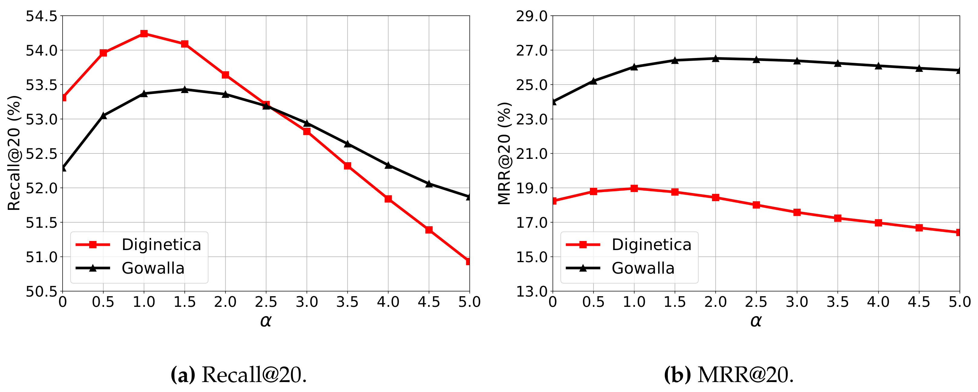
To answer RQ3, we evaluate the performance of DGL-SR with various $\alpha$ in the corrective margin softmax (CMS) on both Diginetica and Gowalla. Specifically, we tune the parameter $\alpha$ in $\{0,0.5,1.0,\dots ,5.0\}$, where the results are shown in Figure 2. Note that when the parameter $\alpha$ is 0, the CMS is the original softmax.

First, from Figure 2, we can observe that the peak value in each performance curve on two datasets can obviously exceed the corresponding performance with the $\alpha$ of 0. This indicates that our proposed corrective margin softmax can address the overfitting problem and improve the recommendation accuracy in terms of Recall@20 and MRR@20 on both datasets. Moreover, when comparing to the performance with the $\alpha$ of 0, we can observe that the improvements brought by the CMS in terms of Recall@20 and MRR@20 are 1.74% and 4.00% on Diginetica, respectively, and the corresponding improvement rates are 2.18% and 10.45% on the Gowalla dataset. We can observe that on both datasets, the improvement is more obvious in terms of MRR@20 than that on Recall@20, indicating that the CMS contributes relatively more to ranking the target items at the right positions.

Moreover, on Diginetica, with $\alpha$ increasing, the performance of DGL-SR in terms of both Recall@20 and MRR@20 first increases and achieves the best performance with the $\alpha$ of 1.0, then begins to consistently decrease. The phenomenon on Gowalla is similar, except that the peak performances are achieved at the $\alpha$ of 1.5 in terms of Recall@20 and 2.0 in terms of MRR@20, respectively. This indicates that the overfitting problem is more serious on Gowalla than that on Diginetica, and the gradient correction is especially necessary for the MRR@20 metric.

5.4. Impact of Training Data Scale

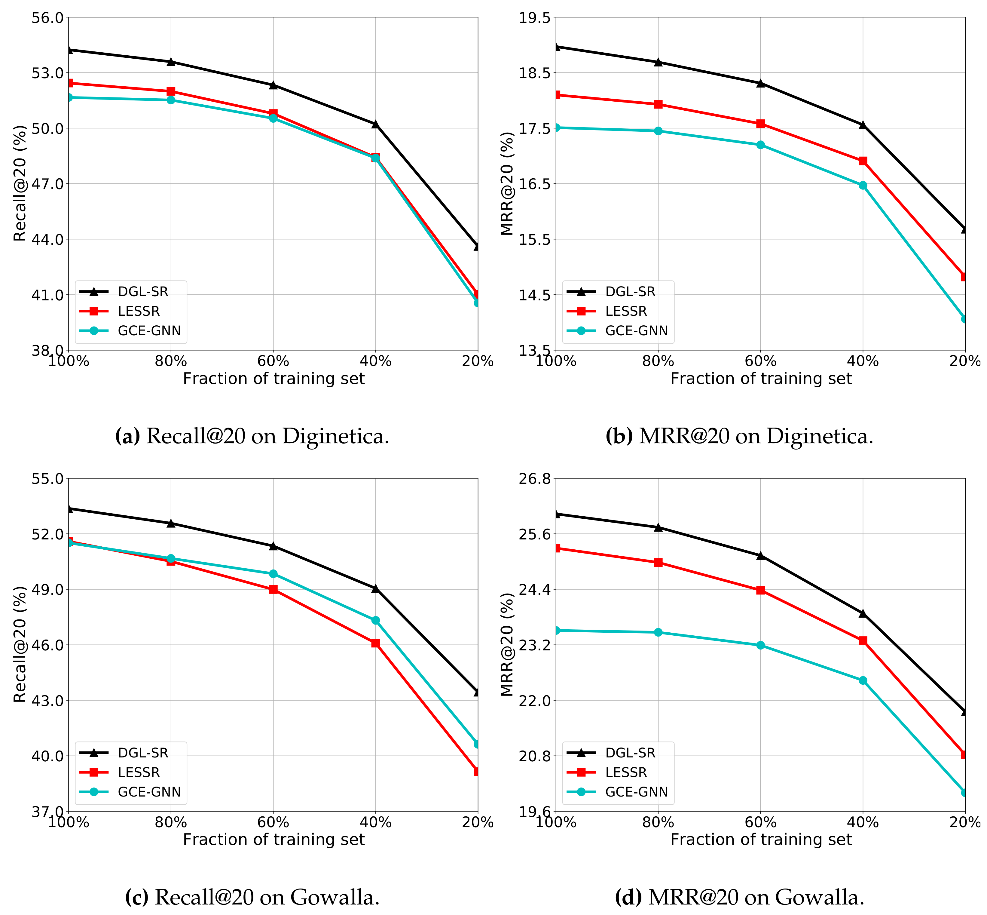
For RQ4, in order to investigate the effectiveness of DGL-SR with different scales of training data available, we compare the performance of DGL-SR with the baselines LESSR and GCE-GNN by using a different fraction of the training set for model optimization. Specifically, we range the fraction in terms of $\{100\%,80\%,60\%,40\%,20\%\}$, and the results are presented in Figure 3.

As for Diginetica, from Figure 3a,b, we can see that our proposed DGL-SR can consistently outperform the baselines on various fractions. Moreover, with the fraction decreasing, the performance of all models in terms of both Recall@20 and MRR@20 consistently decreases, since the transition relation between items is unable to be effectively captured from limited training data. In addition, on the MRR@20 metric, we can observe that the gap between DGL-SR and the best baseline LSEER is relatively more obvious in the large fractions, indicating the utility of our proposal on datasets of a large scale.

On Gowalla, we can observe that the phenomenon is similar to that on the Diginetica dataset. Moreover, comparing the baselines LSEER and GCE-GNN, we can find that GCE-GNN consistently underperforms LESSR in terms of MRR@20 on all fractions; however, the performance gap decreases when the fraction decreases. This may be due to the fact that by exploiting the global transition relation between items, GCE-GNN can effectively slow down the drop in performance when the data fraction decreases. In addition, on the Recall@20 metric, LESSR slightly outperforms GCE-GNN on the “100%” fraction. However, the performance of GCE-GNN begins to exceed LESSR with the deceasing fraction, which means that the static graph constructed from only the ongoing session in LESSR cannot make accurate recommendations with relatively less data for training. On the contrary, our DGL-SR can consistently achieve the best performance on various fractions in terms of both Recall@20 and MRR@20, validating the utility of the dynamic graph learning in scenarios with different amounts of training data.

5.5. Impact of the Session Length

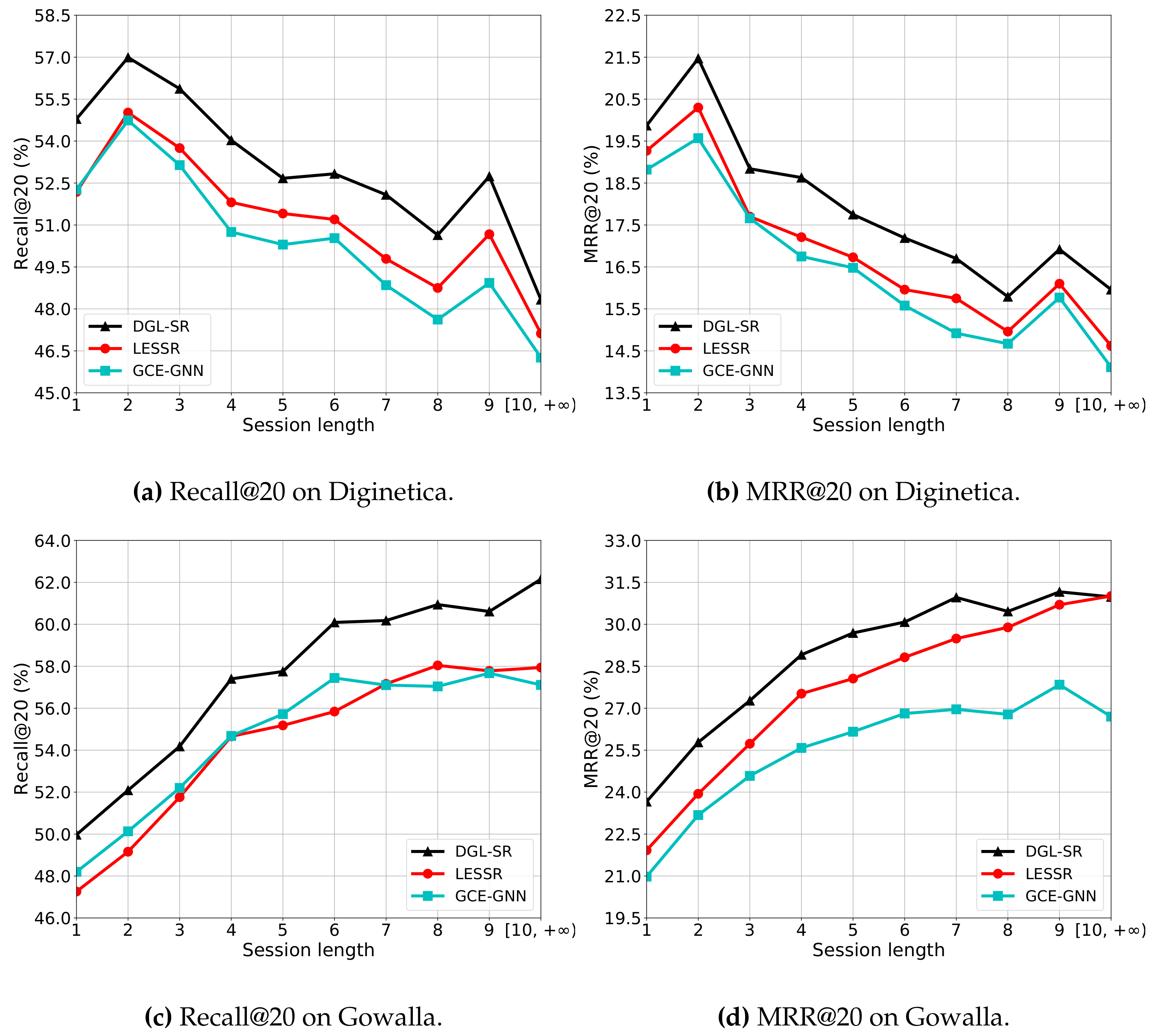
To answer RQ5, we compare the performance of DGL-SR and the baselines LESSR and GCE-GNN on two datasets. Specifically, we evaluate the performance of the models on various session lengths, and the results are shown in Figure 4. First, we can observe that DGL-SR can generally beat the baselines on different lengths in terms of both Recall@20 and MRR@20 on both datasets. This indicates that our proposed DGL-SR can effectively detect the user intent from sessions containing various numbers of items.

For the Diginetica dataset, we can see that the performance of all models in terms of both Recall@20 and MRR@20 first increase from length 1 to 2, and then show consistent decreasing trends. This may be due to the fact that long sessions are likely to include the unrelated items, disturbing the accurate user preference modeling. However, differently on Gowalla, we can see that the performance of all models keep increasing when the session length increases. This indicates that in the check-in scenario, relatively more items can help detect the user intent in the session. Moreover, on the Gowalla dataset, the performance improvements of DGL-SR above the baselines in terms of Recall@20 and MRR@20 are similar on short sessions, however it is more obvious in terms of Recall@20 than that on MRR@20 on long sessions. This indicates that for active users in the check-in scenario, our proposal is relatively more effective on hitting the target item in the recommendation list.

5.6. Hyper-Parameter Study

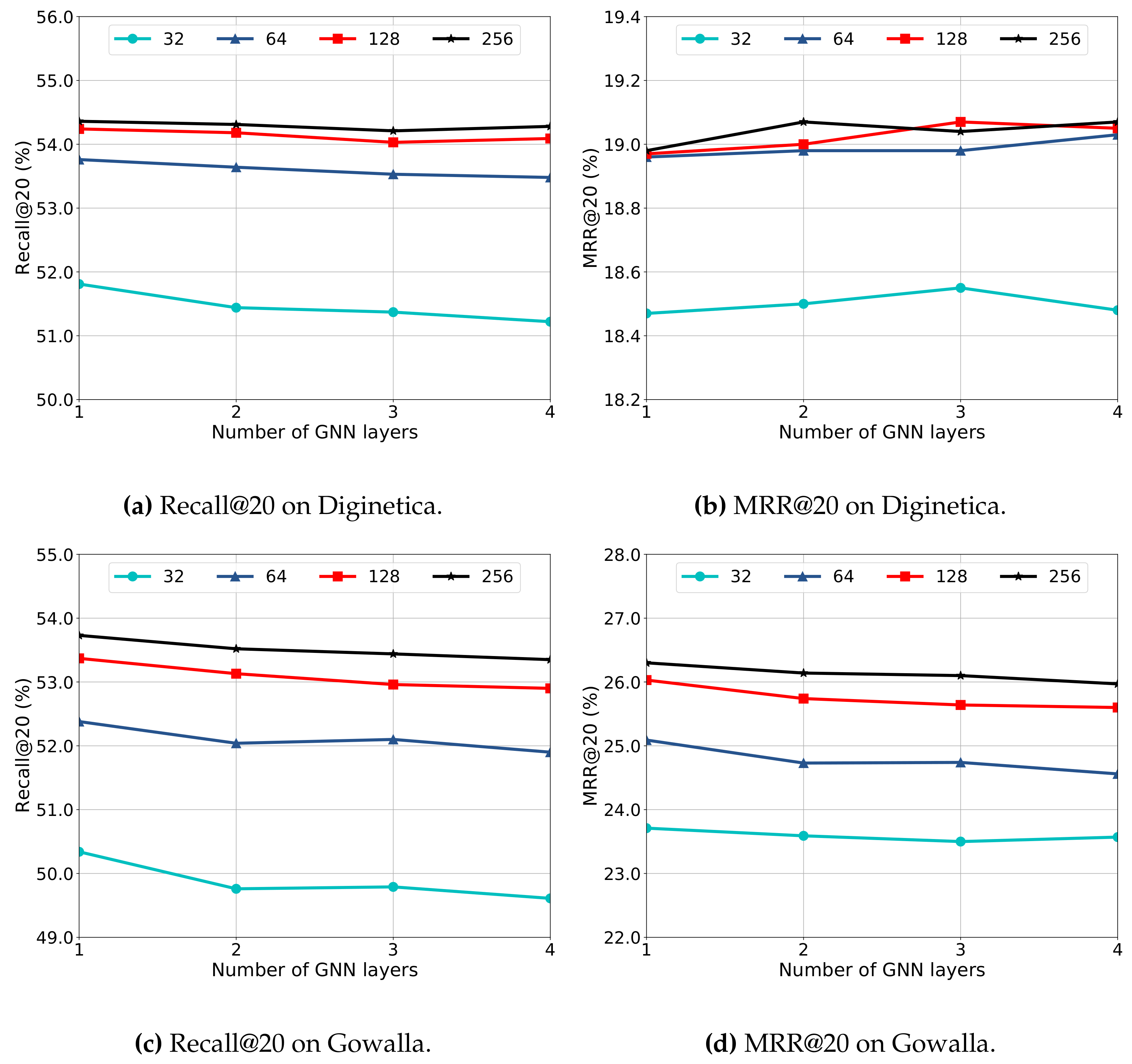
To answer RQ6, we conduct experiments to study the sensitivity of DGL-SR on the GNN layer and the embedding dimension. Specifically, we tune the layer of GNNs in $\{1,2,3,4\}$ and search the embedding dimension in $\{32,64,128,256\}$, respectively. The performance of DGL-SR with different hyper-parameters is presented in Figure 5.

First, as shown in Figure 5, we can observe that increasing the embedding dimension can generally increase the recommendation performance, especially from dimensions 32 to 64. This is because a large embedding dimension has a relatively better representation ability of item characteristics. However, there is a merely limited promotion of the performance when the dimension increases from 128 to 256. Moreover, increasing the embedding dimension will consume more computation resources; thus, the dimension 128 is a proper choice considering both the effectiveness and efficiency of the recommender. Moreover, increasing the GNN layer will generally decrease the model performance on various embedding dimensions in most cases on two datasets, except that the performance slightly increases from layer numbers 1 to 3 on dimensions 32 and 128 in terms of MRR@20 on Diginetica. This could be explained by how the GNNs in session-based recommendation face a serious overfitting problem, as indicated in multiple works [9,17].

5.7. Temporal Attention Visualization

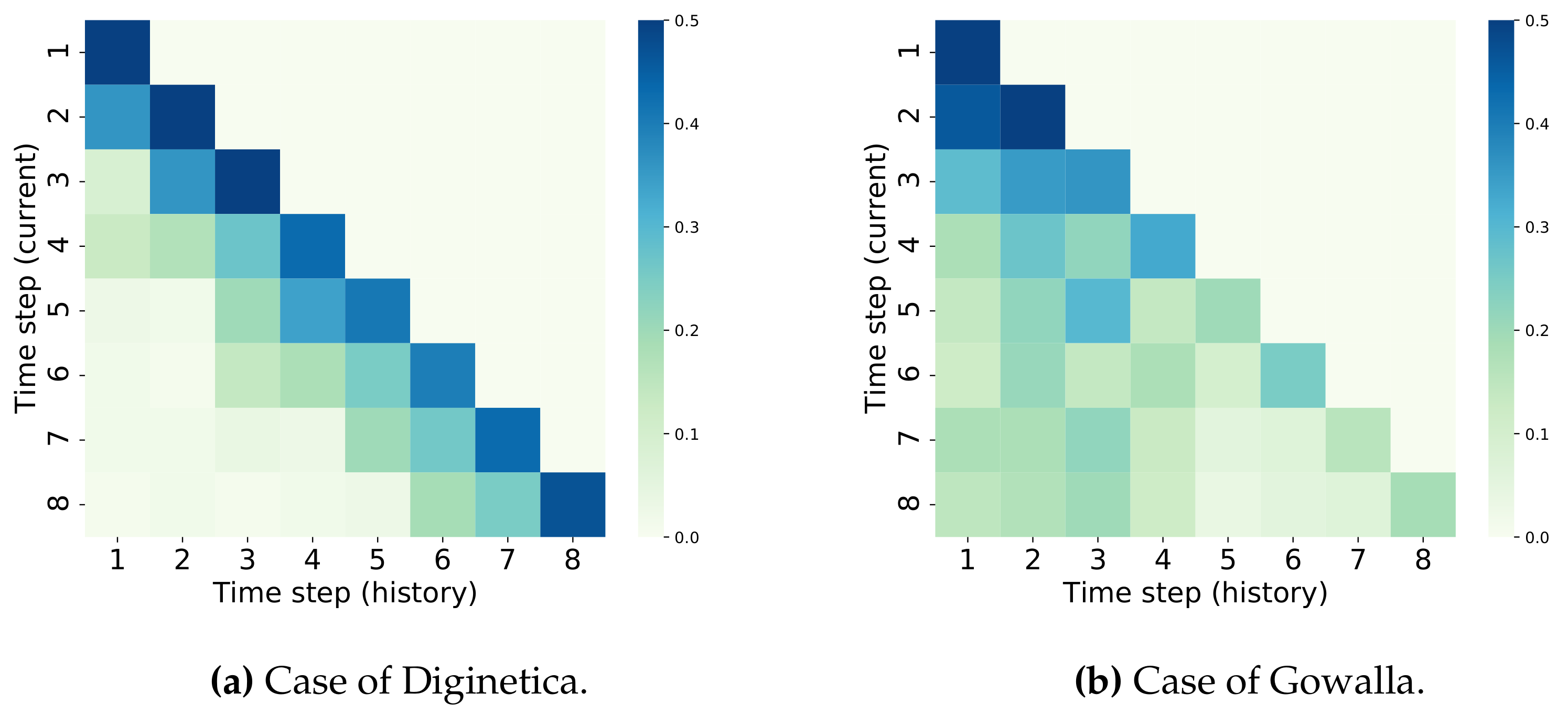
To provide a deep insight into the temporal dynamics in the graph structures over various time-steps of the ongoing session, we conducted a case study which randomly selects a session from Diginetica and Gowalla, respectively. We focus on the eighth item of the two sessions, and show their respective temporal attention weights obtained by Equation (6) in Figure 6. Each row of the attention scores indicates the similarity of the item representation at the current timestamp to that at the historical timestamps, where a deep color indicates a relatively large similarity.

From Figure 6, we can observe that the attention weights in Diginetica tend to be assigned to the recent timestamps; however, it is relatively more uniformly distributed in Gowalla. This may be due to how the impact of the temporal dynamics on the recommendation performance is more obvious on Gowalla than that on Diginetica, which is consistent with the finding in Section 5.2. Moreover, on Gowalla, from the sixth timestamp, the attention weights are larger in the former time-steps than the latter ones, which may be due to how the unrelated items interact after the sixth timestamp, introducing bias into item representation learning. However, through the temporal layer, our proposed DGNN can capture the temporal evolution of the graph structures and dynamically assign weights to the item representations at historical time-steps. Thus, the bias introduced by unrelated items in the ongoing session can be filtered in the user interest detection, so as to accurately learn the user preference.

6. Conclusions and Future Work

In this paper, we proposed a novel approach, that is, dynamic graph learning for session-based recommendation (DGL-SR). DGL-SR applies the dynamic graph neural network (DGNN) to learn the dynamic item representations by taking both the structural information and temporal dynamics of the session graphs at different timestamps into consideration. In addition, we designed a corrective margin softmax (CMS) for the model optimization, which corrects the gradients of the negative samples to alleviate the serious overfitting problem in GNNs for SBRS. Extensive experiments on two benchmark datasets validate the effectiveness of DGL-SR in terms of Recall@20 and MRR@20, especially on hitting the target item in the recommendation list.

As to future work, we would like to investigate the influence of the dwell time between different timestamps of the session graphs on the recommendation accuracy. Moreover, we are also interested in optimizing the model with a limited number of negative samples to reduce the computational cost and speed up the training.

References

- He, X.; Liao, L.; Zhang, H.; Nie, L.; Hu, X.; Chua, T. Neural Collaborative Filtering. In Proceedings of the International World Wide Web Conference (WWW’17), Perth, Australia, 3–7 April 2017; ACM: New York, NY, USA, 2017; pp. 173–182. [Google Scholar]
- Wang, X.; He, X.; Wang, M.; Feng, F.; Chua, T. Neural Graph Collaborative Filtering. In Proceedings of the International ACM SIGIR Conference on Research and Development in Information Retrieval (SIGIR’19), Paris, France, 21–25 July 2019; ACM: New York, NY, USA, 2019; pp. 165–174. [Google Scholar]
- Bhaskaran, S.; Marappan, R.; Santhi, B. Design and Analysis of a Cluster-Based Intelligent Hybrid Recommendation System for E-Learning Applications. Mathematics 2021, 9, 197. [Google Scholar] [CrossRef]
- Zhang, S.; Yao, L.; Sun, A.; Tay, Y. Deep Learning Based Recommender System: A Survey and New Perspectives. ACM Comput. Surv. 2019, 52, 5:1–5:38. [Google Scholar] [CrossRef]
- Wang, S.; Hu, L.; Wang, Y.; Cao, L.; Sheng, Q.Z.; Orgun, M.A. Sequential Recommender Systems: Challenges, Progress and Prospects. In Proceedings of the International Joint Conference on Artificial Intelligence (IJCAI’19), Macao, China, 10–16 August 2019; pp. 6332–6338. [Google Scholar]
- Hidasi, B.; Karatzoglou, A.; Baltrunas, L.; Tikk, D. Session-based Recommendations with Recurrent Neural Networks. In Proceedings of the International Conference on Learning Representations (ICLR’16), San Juan, Puerto Rico, 2–4 May 2016. [Google Scholar]
- Li, J.; Ren, P.; Chen, Z.; Ren, Z.; Lian, T.; Ma, J. Neural Attentive Session-based Recommendation. In Proceedings of the International Conference on Information and Knowledge Management (CIKM’17), Singapore, 6–10 November 2017; ACM: New York, NY, USA, 2017; pp. 1419–1428. [Google Scholar]
- Wang, M.; Ren, P.; Mei, L.; Chen, Z.; Ma, J.; de Rijke, M. A Collaborative Session-based Recommendation Approach with Parallel Memory Modules. In Proceedings of the International ACM SIGIR Conference on Research and Development in Information Retrieval (SIGIR’19), Paris, France, 21–25 July 2019; ACM: New York, NY, USA, 2019; pp. 345–354. [Google Scholar]
- Wu, S.; Tang, Y.; Zhu, Y.; Wang, L.; Xie, X.; Tan, T. Session-Based Recommendation with Graph Neural Networks. In Proceedings of the AAAI Conference on Artificial Intelligence (AAAI’19), Honolulu, HI, USA, 27–28 January 2019; AAAI Press: Palo Alto, CA, USA, 2019; pp. 346–353. [Google Scholar]
- Qiu, R.; Li, J.; Huang, Z.; Yin, H. Rethinking the Item Order in Session-based Recommendation with Graph Neural Networks. In Proceedings of the International Conference on Information and Knowledge Management (CIKM’19), Beijing, China, 3–7 November 2019; ACM: New York, NY, USA, 2019; pp. 579–588. [Google Scholar]
- Wang, Z.; Wei, W.; Cong, G.; Li, X.; Mao, X.; Qiu, M. Global Context Enhanced Graph Neural Networks for Session-based Recommendation. In Proceedings of the International ACM SIGIR Conference on Research and Development in Information Retrieval (SIGIR’20), Virtual Event, China, 25–30 July 2020; ACM: New York, NY, USA, 2020; pp. 169–178. [Google Scholar]
- Liu, Q.; Zeng, Y.; Mokhosi, R.; Zhang, H. STAMP: Short-Term Attention/Memory Priority Model for Session-based Recommendation. In Proceedings of the International Conference on Knowledge Discovery and Data Mining (KDD’18), London, UK, 19–23 August 2018; ACM: New York, NY, USA, 2018; pp. 1831–1839. [Google Scholar]
- Pan, Z.; Cai, F.; Ling, Y.; de Rijke, M. Rethinking Item Importance in Session-based Recommendation. In Proceedings of the International ACM SIGIR Conference on Research and Development in Information Retrieval (SIGIR’20), Virtual Event, China, 25–30 July 2020; ACM: New York, NY, USA, 2020; pp. 1837–1840. [Google Scholar]
- Luo, A.; Zhao, P.; Liu, Y.; Zhuang, F.; Wang, D.; Xu, J.; Fang, J.; Sheng, V.S. Collaborative Self-Attention Network for Session-based Recommendation. In Proceedings of the International Joint Conference on Artificial Intelligence (IJCAI’20), Yokohama, Japan, 11–17 July 2020; pp. 2591–2597. [Google Scholar]
- Rendle, S.; Freudenthaler, C.; Schmidt-Thieme, L. Factorizing personalized Markov chains for next-basket recommendation. In Proceedings of the International World Wide Web Conference (WWW’10), Raleigh, NC, USA, 26–30 April 2010; ACM: New York, NY, USA, 2010; pp. 811–820. [Google Scholar]
- Hidasi, B.; Karatzoglou, A. Recurrent Neural Networks with Top-k Gains for Session-based Recommendations. In Proceedings of the International Conference on Information and Knowledge Management (CIKM’18), Turin, Italy, 22–26 October 2018; ACM: New York, NY, USA, 2018; pp. 843–852. [Google Scholar]
- Pan, Z.; Cai, F.; Chen, W.; Chen, H.; de Rijke, M. Star Graph Neural Networks for Session-based Recommendation. In Proceedings of the International Conference on Information and Knowledge Management (CIKM’20), Virtual Event, Ireland, 19–23 October 2020; ACM: New York, NY, USA, 2020; pp. 1195–1204. [Google Scholar]
- Ma, X.; Dong, L.; Wang, Y.; Li, Y.; Sun, M. AIRC: Attentive Implicit Relation Recommendation Incorporating Content Information for Bipartite Graphs. Mathematics 2020, 8, 2132. [Google Scholar] [CrossRef]
- Li, Y.; Tarlow, D.; Brockschmidt, M.; Zemel, R.S. Gated Graph Sequence Neural Networks. In Proceedings of the International Conference on Learning Representations (ICLR’16), San Juan, Puerto Rico, 2–4 May 2016. [Google Scholar]
- Kang, W.; McAuley, J.J. Self-Attentive Sequential Recommendation. In Proceedings of the IEEE International Conference on Data Mining (ICDM’18), Singapore, 17–20 November 2018; IEEE Computer Society: Washington, DC, USA, 2018; pp. 197–206. [Google Scholar]
- Chen, T.; Wong, R.C. Handling Information Loss of Graph Neural Networks for Session-based Recommendation. In Proceedings of the International Conference on Knowledge Discovery and Data Mining (KDD’20), Virtual Event, CA, USA, 6–10 July 2020; ACM: New York, NY, USA, 2020; pp. 1172–1180. [Google Scholar]
- Li, A.; Huang, W.; Lan, X.; Feng, J.; Li, Z.; Wang, L. Boosting Few-Shot Learning With Adaptive Margin Loss. In Proceedings of the IEEE/CVF Conference on Computer Vision and Pattern Recognition (CVPR’20), Seattle, WA, USA, 13–19 June 2020; IEEE: Piscataway, NJ, USA, 2020; pp. 12573–12581. [Google Scholar]
- Shani, G.; Heckerman, D.; Brafman, R.I. An MDP-Based Recommender System. J. Mach. Learn. Res. 2005, 6, 1265–1295. [Google Scholar]
- Jannach, D.; Ludewig, M. When Recurrent Neural Networks meet the Neighborhood for Session-Based Recommendation. In Proceedings of the ACM Conference on Recommender Systems (RecSys’17), Como, Italy, 27–31 August 2017; ACM: New York, NY, USA, 2017; pp. 306–310. [Google Scholar]
- Pan, Z.; Cai, F.; Ling, Y.; de Rijke, M. An Intent-guided Collaborative Machine for Session-based Recommendation. In Proceedings of the International ACM SIGIR Conference on Research and Development in Information Retrieval (SIGIR’20), Virtual Event, China, 25–30 July 2020; ACM: New York, NY, USA, 2020; pp. 1833–1836. [Google Scholar]
- Ren, P.; Chen, Z.; Li, J.; Ren, Z.; Ma, J.; de Rijke, M. RepeatNet: A Repeat Aware Neural Recommendation Machine for Session-Based Recommendation. In Proceedings of the AAAI Conference on Artificial Intelligence (AAAI’19), Honolulu, HI, USA, 27–28 January 2019; AAAI Press: Palo Alto, CA, USA, 2019; pp. 4806–4813. [Google Scholar]
- Wang, B.; Cai, W. Attention-Enhanced Graph Neural Networks for Session-Based Recommendation. Mathematics 2020, 8, 1607. [Google Scholar] [CrossRef]
- Vinyals, O.; Bengio, S.; Kudlur, M. Order Matters: Sequence to sequence for sets. In Proceedings of the International Conference on Learning Representations (ICLR’16), San Juan, Puerto Rico, 2–4 May 2016. [Google Scholar]
- Xu, C.; Zhao, P.; Liu, Y.; Sheng, V.S.; Xu, J.; Zhuang, F.; Fang, J.; Zhou, X. Graph Contextualized Self-Attention Network for Session-based Recommendation. In Proceedings of the International Joint Conference on Artificial Intelligence (IJCAI’19), Macao, China, 10–16 August 2019; pp. 3940–3946. [Google Scholar]
- Gupta, P.; Garg, D.; Malhotra, P.; Vig, L.; Shroff, G.M. NISER: Normalized Item and Session Representations with Graph Neural Networks. arXiv 2019, arXiv:1909.04276. [Google Scholar]
- Rumelhart, D.E.; Hinton, G.E.; Williams, R.J. Learning representations by back-propagating errors. Nature 1986, 323, 533–536. [Google Scholar] [CrossRef]
- Guo, L.; Yin, H.; Wang, Q.; Chen, T.; Zhou, A.; Hung, N.Q.V. Streaming Session-based Recommendation. In Proceedings of the International Conference on Knowledge Discovery and Data Mining (KDD’19), London, UK, 4–8 August 2019; ACM: New York, NY, USA, 2019; pp. 1569–1577. [Google Scholar]
- Qiu, R.; Yin, H.; Huang, Z.; Chen, T. GAG: Global Attributed Graph Neural Network for Streaming Session-based Recommendation. In Proceedings of the International ACM SIGIR Conference on Research and Development in Information Retrieval (SIGIR’20), Virtual Event, China, 25–30 July 2020; ACM: New York, NY, USA, 2020; pp. 669–678. [Google Scholar]
- Davidson, J.; Liebald, B.; Liu, J.; Nandy, P.; Vleet, T.V.; Gargi, U.; Gupta, S.; He, Y.; Lambert, M.; Livingston, B.; et al. The YouTube video recommendation system. In Proceedings of the ACM Conference on Recommender Systems (RecSys’10), Barcelona, Spain, 26–30 September 2010; ACM: New York, NY, USA, 2010; pp. 293–296. [Google Scholar]
- Yuan, F.; Karatzoglou, A.; Arapakis, I.; Jose, J.M.; He, X. A Simple Convolutional Generative Network for Next Item Recommendation. In Proceedings of the International Conference on Web Search and Data Mining (WSDM’19), Melbourne, Australia, 11–15 February 2019; ACM: New York, NY, USA, 2019; pp. 582–590. [Google Scholar]