Formalizing Calculus without Limit Theory in Coq

Abstract

Formal verification of mathematical theory has received widespread concern and grown rapidly. The formalization of the fundamental theory will contribute to the development of large projects. In this paper, we present the formalization in Coq of calculus without limit theory. The theory aims to found a new form of calculus more easily but rigorously. This theory as an innovation differs from traditional calculus but is equivalent and more comprehensible. First, the definition of the difference-quotient control function is given intuitively from the physical facts. Further, conditions are added to it to get the derivative, and define the integral by the axiomatization. Then some important conclusions in calculus such as the Newton–Leibniz formula and the Taylor formula can be formally verified. This shows that this theory can be independent of limit theory, and any proof does not involve real number completeness. This work can help learners to study calculus and lay the foundation for many applications.

1. Introduction

As proof assistants Coq [1,2,3], Isabelle [4] and HOL [5] and so on [6,7,8,9] develop, formal mathematics has achieved considerable progress [10,11,12,13]. In 2005, Gonthier and Werner proved the famous “Four Color theorem” [11] in a fully formal way. Further, Gonthier presented the formal proof of the “Odd Order Theorem” [12] in 2012. In 2017, Hales et al. formalized “Kepler Conjecture” [13] to verify his previous proof [14]. In 2019, Cruz-Filipe et al. completed the formalization of the “Boolean Pythagorean Triples Problem” [10], which checked the development of Marijn et al. [15]. Those achievements make formal mathematics recognized and advocated by mathematicians [16,17]. Moreover, the formalizations require mathematical understanding and familiarity with tools, and the use of developed libraries in a variety of proof assistants. Formalizing the fundamental theory will contribute to the development of large projects.

As one of the milestone accomplishments in mathematics history, calculus was founded more than 300 years ago. It greatly promoted the development of mathematics and other scientific fields, and solved many problems in practical engineering. Newton and Leibniz first created calculus, which settled many historical mathematical problems at that time and made a profound influence. Due to the concept of vague infinitesimal, however, it was questioned and this caused the second mathematical crisis.

Lagrange endeavored to establish the whole calculus theory on Taylor formula to avoid dealing with Newton’s “fluxion”, and Leibniz’s “infinitesimal”, but the convergence of infinite series still could not avoid the concept of limit. Until the 19th century, the progress of analysis led mathematicians to establish a rigorous limit theory [18]. The landmark work was mainly conducted by Cauchy [19], Bolzano [20] and Weierstrass [21], and defined the limit strictly by “$ϵ$-N”. This theory fundamentally solves the second mathematical crisis and has become a solid foundation of modern analysis. Because of complicated concepts and reasoning, however, it is hard for some beginners to absorb and understand.

In order to enable learners to study calculus theory with less time and energy, several scholars [22,23,24,25,26,27] constantly strive to establish a new theory. By researching calculus in depth, this idea became a reality and considerable progress has been made [23,26,28,29]. “The limit theory is not a prerequisite for learning calculus, and high school students with knowledge of function can understand the majority of calculus topics” [30]. The calculus without limit theory can help beginners to learn more quickly, more easily, and more effectively, by the relationship between calculus concepts and the physical world, to rapidly master the most critical skills in calculus and settle some problems in mathematics and real life [30,31,32].

The calculus without limit theory can be founded rigorously and comprehensibly. Moreover, most propositions whose proof needs to involve completeness, continuity and limit in traditional calculus can be proved directly in this theory. This does not mean, however, that limit theory should never be learned [30,33]. Calculus relying on real number theory and limit theory is undoubtedly a qualitative leap in the history of mathematics. Actually, it is beneficial to learn limit theory to grasp some calculus knowledge much better and much more deeply. Thus, formalizing the calculus without limit theory has particular significance for teaching and research.

Our formalization draws lessons from all the former works and sorts out a more complete and systematic version. This work is based on the formal system of Landau’s “Foundations of Analysis” [34] developed by ourselves. There is very little preparatory knowledge required in this monograph. Starting from the Peano axioms, the whole theory of the number system from natural numbers to complex numbers is given in turn. As an application of our system, we formally completed the cyclic proof of eight completeness theorems and the proof of properties of a continuous function on closed intervals [35,36]. It should be noted that we only use the contents before Section 4.4 which do not involve completeness (Dedekind fundamental theorem) yet.

In this work, the concept of difference-quotient control function is first introduced from motion law. Next, the elementary definitions of uniform derivative and strong derivative can be naturally obtained. Then, the integral system and definite integral are given by axiomatization. At the same time, we discuss the relationship between them. Furthermore, we present the related concept of higher order derivative. At last, some important theorems in calculus can be directly proved, and this suggests that this theory does not rely on real number completeness and limit theory. On the one hand, every proof is verified by Coq to show rigor and correctness. On the other hand, we make up for missing proof details to make it more complete. In addition, there are some innovations of formal methods in the proof process. The proofs are checked formally using the Coq proof assistant, and the machine proving progress is rigorous and reliable.

The paper is organized in the following way. Section 2 is dedicated to related work. Section 3 briefly states the necessary background needed for understanding this work. Section 4 introduces some definitions and consequences concerning them needed in establishing the theory. Section 5 presents the formalization of calculus without limit theory. Section 6 describes the definition of higher order derivative and related properties. Section 7 discusses the proof of critical theorems in calculus. Finally, we draw our conclusions and discuss some potential further work in Section 8.

2. Related Work

In the 1960s, Ljusternik et al. [25] proposed the concept of uniformly derivable, which can be proved to be equivalent to the concept of continuously derivable. They used this concept to simplify the calculus reasoning, but the process still depended on the limit. In 1999, Dovermann [22] introduced the concept of differentiability without limit based on the Lipschitz condition so that his students could quickly learn the calculus theory. At the same time, he admitted that the differentiability introduced by him was not rigorous compared to traditional calculus theory. Later, Lin [23,28] pointed out that the fundamental theorem of calculus can be simplified by consistent derivative. Further he explicitly put forward the uniform inequality as the primary definition of derivative, which can be used as a new guide to calculus without limit theory. In 2005, Sparks [26] avoided the limit concept in his book “Calculus Without Limits”, where the basic concepts and calculus formulas are explained with simple examples. This is an outstanding progression of calculus without limit theory; however, he did not form a systematic and complete theory. After that, Livshits [24,37] proposed a method to directly define differential and integral without depending on real number completeness, limit and continuity. This work is also based on the concept of the differentiability of the Lipschitz function. On the other hand, Zhang [27,29,38,39,40] introduced the concept that the difference quotient of one function is the median of another function, which shows the relationship between a function and its derivative and the integral in essence. This theory gives the intuitive definition of an integral system and reveals the necessary and sufficient conditions for uniform derivative and strong derivative. Thus the calculus system without limit can be established wholly and rigorously. In recent years, Zhang and Tong [30] proposed the difference-quotient control function based on the previous concept, and they gave a new concept of macro derivative. Together with them, Lin [31,32,33] supplements the real number axioms and function continuity to enrich the theory.

There already exist some formalizations of Landau’s “Foundations of Analysis” [41,42,43]. A little different from them, we implement the formalizations strictly following the monograph based on Coq. On the other hand, Cruz-Filipe et al. developed the Constructive Coq repository, C-CoRN [44,45], and Boldo et al. developed the excellent real analysis library—Coquelicot [46]—as an extension of the standard library. Both developments are based on real number completeness and limit theory.

Our previous paper [47] formalized all definitions and theorems of the paper [39], and the development completely corresponds to the structure of the paper. Compared with this work, there are innovations in the following aspects that have been made. We systematically formalize calculus without limit theory based on the existing research results [27,29,30,31,39,47]. The development is built on our system rather than the standard library. Moreover, it only uses the contents before Section 4.4 [34], which does not involve completeness (Dedekind fundamental theorem) yet. Consequently, this does verify that the calculus without limit theory does not need to introduce a completeness theorem. Starting from the difference-quotient control function, we introduce derivative and integral and discuss the relationship between them, which is more natural and clear. Besides adding some properties that have not been proved before, the theorems in calculus for uniform derivative can be obtained, and further these theorems for strong derivative can be easily deduced. At last, we use several notations to improve readability and optimize the size of the proofs.

3. Preliminary

3.1. Coq

The Coq system uses a very expressive variation on typed $\lambda$-calculus, the Calculus of Inductive Constructions [48,49,50]. For the sake of readability, we use “$\forall ,\exists$” to represent universal quantifiers and existential quantifiers, and “$\lambda t,\dots$” to represent anonymous function “fun $t=>\dots$” in Coq. It is based on intuitionism, and some logical axioms can be introduced in developments without contradiction (The key axioms of Coq is available at https://github.com/coq/coq/wiki/CoqAndAxioms accessed on 15 May 2019). In the formalization of “Foundations of Analysis”, three logical axioms are introduced, and they are described in Coq as follows:

Axiom classicT : ∀ P, {P} + {~P}.
		Axiom prop_ext : ∀ P Q, P <-> Q -> P = Q.
		Axiom fun_ext : ∀ {T1 T2 :Type} (P Q :T1 -> T2), (∀ m, P m = Q m) -> P = Q.
		

The first one can be used to build the piecewise function according to the correctness of the proposition, and the definition of real addition uses it first. The second one states that equivalent propositions can be replaced by each other, and further, we can derive proof irrelevance which is necessary to substitute equivalent types in proofs. The last one [51] that is similar to the equality of functions in set theory [52] is used to prove the equality of functions in type theory, and it can combine with the second axiom to prove the predicate extensionality as follows:

		∀ {A :Type} {P :A -> Prop}, (∀ a, P a ↔ Q a) → P = Q.
		

In addition, more details are discussed in Section 3.2 of our paper [36].

In the formalization of calculus without limit theory, another axiom needs to be introduced to instantiate an existing variable that cannot be constructed. This axiom called “cid” is short for “constructive_indefinite_description” in the standard library, and we can define the function to get an element satisfying a specific property by it. This function appears only in definitions or theorem statements because in propositional proofs we “elim” the existential to get an existential witness. The formal descriptions are as follows:

Axiom cid : ∀ {A :Type} {P :A -> Prop}, (∃ x, P x) -> { x :A | P x }.
        Definition Getele {A :Type} {P :A -> Prop} (Q :∃ x, P x) ≔ proj1_sig (cid Q).

3.2. Real Number Theory System

Landau’s “Foundations of Analysis” [34] is based on set theory [52] and some basic logic. Starting from the Peano axioms, the whole theory of the number system from natural numbers to complex numbers is given in turn. It should be noted that we only use the contents before Section 4.4, which does not involve completeness (Dedekind fundamental theorem) yet.

This system formalizes the set of strictly positive natural numbers, i.e., natural numbers without zero. For readability, “1” means One, and “x”’ means the successor of x. The formalization of the set of strictly positive natural numbers is as follows:

Inductive Nat : Type ≔
		  | One
          | Successor : Nat -> Nat.
        Notation "1" ≔ One.
        Notation " x ‘ " ≔ (Successor x)(at level 0).
		

Then the whole formalization strictly follows Landau’s “Foundations of Analysis”, and we do not discuss it in detail. If you are interested, the complete source is available online

https://github.com/coderfys/Analysis/tree/main/Foundations_of_Analysis/, accessed on 10 June 2021

The definitions of some operations are different from the traditional ones. For example, natural number subtraction is a partial function; the definition of subtraction needs three input parameters: Two natural numbers and a proof that the second one is less than the first one. For example, “$x-y$ l” represents “x minus y” and “l” is a proof of “$x>y$”. Meanwhile, we can add the notations to real number operations, which automatically override and invalidate the previous notations. Thus the operation symbol in this paper refers to real number operation, and a code like “operation_type” represents the naming rule for different types of operations.

Table 1. The meaning of the code in real number theory system.

Code	Meanning
$a\in A$	a is an element of the set A
Minus_N $xyl$	x minus y, l is proof “$x>y$” , x and y are natural numbers
$a+b$	a plus b
$a-b$	a minus b
$\left|a\right|$	absolute value of a
$a·b$	a times b
factorial n	$n!$, n is a natural number
$a^{\wedge }n$	$a^n$, n is a natural number
$(a/b)l$	a divide into b, l is proof “b <> 0”
RdiN $rN$	$\frac{r}{N}$, N is a natural number
Rdifa $rN$	$\frac{r}{N!}$, N is a natural number
$\left[a\right|b],(a\left|b\right]$	$[a,b]$, $(a,b]$
maxfun $fg$	$max\left\{f\right(x),g(x\left)\right\}$

below is convenient for understanding the system, and the variables are real numbers without a particular description.

4. Basic Definitions and Properties

The formal definition of the real valued function is as follows:

Definition RFun ≔ Real -> Real.
      

We define a conversion from a univariate function to a bivariate function like this: $F\#(u,v)=F\left(v\right)-F\left(u\right)$. This function can be used to get the fact that $F\left(x\right)=G\left(x\right)+C$ if and only if $F\#(u,v)=G\#(u,v)$. It is formally defined is as follows:

Definition input2Mi (F :Rfun) ≔ λ u v, F(v) - F(u).
      Notation "F #" ≔ (input2Mi F)(at level 5).
      

The identical function and constant function are represented by $\Delta ,\mathrm{\Phi }\left(C\right)$. They are defined in Coq as follows:

Definition Δ :Rfun ≔ λ x, x.
	  Definition ϕ :Real -> Rfun ≔ λ C, (λ _, C).
      

Here are the formalizations of function operations ($cf\left(x\right)$, $f\left(cx\right)$, $f(cx+d)$, $-f\left(x\right)$, $f\left(x\right)+g\left(x\right)$, $f\left(x\right)-g\left(x\right)$, $f\left(x\right)·g\left(x\right)$, max$\left\{f\right(x),g(x\left)\right\}$) as follows:

Definition mult_fun c (f :Rfun) ≔ λ x, c · f(x).
        Definition multfun_ (f :Rfun) c ≔ λ x, f(c · x).
        Definition multfun_pl (f :Rfun) c d ≔ λ x, f(c · x + d).
        Definition minus_fun (f :Rfun) ≔ λ x, - f(x).
        Definition Plus_Fun (f g :Rfun) ≔ λ x, f(x) + g(x).
        Definition Minus_Fun (f g :Rfun) ≔ λ x, f(x) - g(x).
        Definition Mult_Fun (f g :Rfun) ≔ λ x, f(x) · g(x).
        Definition maxfun (f g :Rfun) ≔
          λ x, match (Rcase (f x)(g x)) with
                | left _ => g x
                | right _ => f x
               end.
      

The formalizations of increasing (strictly) function and decreasing (strictly) function are as follows:

Definition fun_inc f I ≔ ∀ x y, x ∈ I -> y ∈ I -> x < y -> f x ≤ f y.
      Definition fun_sinc f I ≔ ∀ x y, x ∈ I -> y ∈ I -> x < y -> f x < f y.
      Definition fun_dec f I ≔ ∀ x y, x ∈ I -> y ∈ I -> x < y -> f y ≤ f x.
      Definition fun_sdec f I ≔ ∀ x y, x ∈ I -> y ∈ I -> x < y -> f x > f y.
      Definition convexdown f I ≔ ∀ x1 x2, x1 ∈ I -> x2 ∈ I ->
        ∀ c, c > O -> c < 1 -> f(c·x1+(1-c)·x2) ≤ c·f(x1) + (1-c)·f(x2).
      Definition convexup f I ≔ ∀ x1 x2, x1 ∈ I -> x2 ∈ I ->
        ∀ c, c > O -> c < 1 -> c·f(x1) + (1-c)·f(x2) ≤ f(c·x1+(1-c)·x2).
      

Here are the formalizations of positive value increasing function, unbounded reciprocal function and bounded function as follows.

Definition fun_pinc f I ≔ (∀ z, z ∈ I -> f z > O) /\ fun_inc f I.
        Definition unbRecF (f :Rfun) I ≔ ∀ M, ∃ z l, z ∈ I /\ M < |(1/(f z)) l|.
        Definition bound_ran f a b ≔ ∃ A, A > O /\ ∀ x, x ∈ [a|b] -> |f x| < A.
      

We can get some propositions from the above definitions. The identical mapping is a positive value increasing function and an unbounded reciprocal function. If both $d_1$ and $d_2$ are positive value increasing functions, then max$\{d_1,d_2\}$ is a positive value increasing function, and further, if both $d_1$ and $d_2$ are also unbounded reciprocal functions, then max$\{d_1,d_2\}$ is an unbounded reciprocal function. Additionally, if d is a positive value increasing function and a function f such that $\forall x,x+h\in [a,b],\left|f\right(x+h)-f(x\left)\right|\le d\left(\right|h\left|\right)$, then f is a bounded function.

Fact fpcp1 : ∀ a b, fun_pinc Δ (O|b-a].
        Fact fpcp2 : ∀ {d1 d2 R},
          fun_pinc d1 R -> fun_pinc d2 R -> fun_pinc (maxfun d1 d2) R.
        Fact ubrp1 : ∀ {a b}, a~< b -> unbRecF Δ (O|b-a].
        Fact ubrp2 : ∀ {d1 d2 R}, fun_pinc d1 R -> fun_pinc d2 R ->
          unbRecF d1 R -> unbRecF d2 R -> unbRecF (maxfun d1 d2) R.
        Fact brp1 : ∀ {f d a b}, fun_pinc d (O|b-a] ->
          (∀ x h, x ∈ [a|b] -> (x+h) ∈ [a|b] -> |f(x+h) - f(x)| ≤ d(|h|)) ->
          bound_ran f a b.
      

Moreover, we define a uniformly continuous function by two definitions above. It is defined in Coq as follows:

Definition uniform_continuous f a b ≔
          ∃ d, fun_pinc d (O|b-a] /\ unbRecF d (O|b-a] /\
          ∀ x h, x ∈ [a|b] -> (x+h) ∈ [a|b] -> |f(x+h) - f(x)| ≤ d(|h|).
      

Furthermore, we can get that if f is uniformly continuous on $[a,b]$, then $a<b$ and f is bounded.

Fact uclt : ∀ {f a b}, uniform_continuous f a b -> a < b.
        Fact ucbound : ∀ {f a b}, uniform_continuous f a b -> bound_ran f a b.
		

Here is the formalization of a Lipschitz function as follows.

Definition Lipschitz f a b ≔
          ∃ M, M > O /\ ∀ x h, x ∈ [a|b] -> (x+h) ∈ [a|b] -> |f(x+h) - f(x)| ≤ M·|h|.
      

Further, we can prove that a function is bounded.

Fact lipbound : ∀ {f a b}, Lipschitz f a b -> bound_ran f a b.
      

5. Differential and Integral

“Calculus without limit theory is founded upon two physical facts: (1) an average velocity is always between two instantaneous velocities; (2) the motion of an object is determined once its velocity has been determined” [30]. So we first give the concept of difference-quotient control function, which can reflect the motion law directly. Further, we can define the uniform derivative and the strong derivative that are both closely related to the difference-quotient control function. At last, we present the integral system and the definite integral, and further, we discuss the relationship between difference-quotient control function and them. These embody the importance of the difference-quotient control function in this theory.

5.1. Difference-Quotient Control Function

Let functions F and f be defined on $[a,b]$. If $\forall u<v\in [a,b]$, there exist $p,q\in [u,v]$ such that

$$f\left(p\right)\le \frac{F\left(v\right)-F\left(u\right)}{v-u}\le f\left(q\right)$$

then the function f is called the difference-quotient control function (DCF) of F on $[a,b]$.

Its formalization is as follows (as shown in Table 1, “uneqOP l” is the proof of “$v-u\ne 0$” where “l” is the proof of “$v-u>0$” and the “uneqOP” function represents that no positive number is zero):

Definition diff_quo_median F f a b ≔
            ∀ u v l, u ∈ [a|b] -> v ∈ [a|b] -> ∃ p q, p ∈ [u|v] /\ q ∈ [u|v] /\
            f p ≤ ((F v - F u)/(v-u))(uneqOP l) /\ ((F v - F u)/(v-u))(uneqOP l) ≤ f q.
        

Let f be the DCF of F on $[a,b]$, then we can obtain some conclusions as follows:

• $\mathrm{\Phi }\left(0\right)$ is the DCF of a constant function,
• $\mathrm{\Phi }\left(C\right)$ is the DCF of a linear function,
• $cf\left(x\right)$ is the DCF of $cF\left(x\right)$ on $[a,b]$,
• $-f(-x)$ is the DCF of $F(-x)$ on $[-b,-a]$,
• $cf(cx+d)$ is the DCF of $F(cx+d),c>0$ on $[\frac{a-d}{c},\frac{b-d}{c}]$.

Their formalizations are as follows:

Fact medC : ∀ a b C, diff_quo_median (ϕ(C)) (ϕ(O)) a b.
          Fact medCx : ∀ a b C, diff_quo_median (λ x, C·x) (ϕ(C)) a b.
          Fact medfMu : ∀ {a b F f} c, diff_quo_median F f a b ->
            diff_quo_median (mult_fun c F) (mult_fun c f) a b.
          Fact medf_mi : ∀ {F f a b}, diff_quo_median F f a b ->
            diff_quo_median (λ x, F(-x)) (λ x, -f(-x)) (-b) (-a).
          Fact medf_cd : ∀ {F f a b} c d l,
            diff_quo_median F f a b -> diff_quo_median (multfun_pl F c d)
            (mult_fun c (multfun_pl f c d))(((a-d)/c) (uneqOP l))(((b-d)/c) (uneqOP l)).
        

Next, we can get the relation between DCF and monotonicity, concavity.

• If $f\left(x\right)\ge 0\left(f\right(x)\le 0)$ in I, then F is increasing(decreasing) in I,
• If $f\left(x\right)>0\left(f\right(x)<0)$ in I, then F is strictly increasing(decreasing) in I,
• If f is increasing(decreasing) in I, then F is convex down(convex up) in I.

Their formalizations are as follows:

Fact medpos_inc : ∀ F f a b,
            diff_quo_median F f a b -> (∀ x, x ∈ [a|b] -> f(x) ≥ O) -> fun_inc F [a|b].
          Fact medneg_dec : ∀ F f a b,
            diff_quo_median F f a b -> (∀ x, x ∈ [a|b] -> f(x) ≤ O) -> fun_dec F [a|b].
          Fact medpos_sinc : ∀ F f a b,
            diff_quo_median F f a b -> (∀ x, x ∈ [a|b] -> f(x) > O) -> fun_sinc F [a|b].
          Fact medneg_sdec : ∀ F f a b,
            diff_quo_median F f a b -> (∀ x, x ∈ [a|b] -> f(x) < O) -> fun_sdec F [a|b].
          Fact medconc :
            ∀ {F f a b}, diff_quo_median F f a b -> fun_inc f [a|b] -> convexdown F [a|b].
          Fact medconv :
            ∀ {F f a b}, diff_quo_median F f a b -> fun_dec f [a|b] -> convexup F [a|b].
        

The proof of the first four propositions can be easily obtained, and we discuss the proof of the last two propositions in detail. Let f be the DCF of F on $[a,b]$.

Supposing f is increasing on $[a,b]$. We first prove the lemma whose formalization is as follows:

Lemma medccpre : ∀ {F f a b}, diff_quo_median F f a b ->
            fun_inc f [a|b] -> ∀ {x1 x2}, x1 < x2 -> x1 ∈ [a|b] -> x2 ∈ [a|b] ->
            ∀ c, c > O -> c < 1 -> F(c·x1+(1-c)·x2) ≤ c·F(x1) + (1-c)·F(x2).
        

Proof. 

Let “y” be equal to “$c{x}_1+(1-c)x_2$”. We can prove that $y-x_1>0,x_2-y>0$, then $y\in [a,b]$. From the definition of DCF, there exist $p_1,q_1\in [x_1,y],p_2,q_2\in [y,x_2]$, such that

$$f\left(p_1\right)\le \frac{F\left(y\right)-F\left(x_1\right)}{(1-c)(x_2-x_1)}\le f\left(q_1\right),f\left(p_2\right)\le \frac{F\left(x_2\right)-F\left(y\right)}{c(x_2-x_1)}\le f\left(q_2\right)$$

We multiply the two sides of the inequalities by $c(1-c)(x_2-x_1)$, and we get

$$c(F\left(y\right)-F\left(x_1\right))\le c(1-c)(x_2-x_1)f\left(q_1\right),$$

$$c(1-c)(x_2-x_1)f\left(p_2\right)\le (1-c)(F\left(x_2\right)-F\left(y\right))$$

We can obtain $c(F\left(y\right)-F\left(x_1\right))\le (1-c)(F\left(x_2\right)-F\left(y\right))$ since $q_1\le p_2\in [x_1,x_2]$ and f is increasing. Then we can get $F\left(y\right)\le cF\left(x_1\right)+(1-c)F\left(x_2\right)$ by transposition; so this case is proved.

If $x_1=x_2$, the inequality is reduced to “$F\left(x_1\right)\le F\left(x_1\right)$”, which is obviously true. If $x_2<x_1$, we can get that $F(c{x}_2+(1-c)x_1)\le cF\left(x_2\right)+(1-c)F\left(x_1\right)$ from case “$x_1<x_2$”. We just let “d” be equal to “$1-c$”; then $F(d{x}_1+(1-d)x_2)\le dF\left(x_1\right)+(1-d)F\left(x_2\right)$. So the proposition is proved.

Supposing f is decreasing on $[a,b]$. First, we can get that $-f\left(x\right)$ is increasing, and further, by the conclusion above, we can prove that

$$-F(c{x}_1+(1-c)x_2)\le -cF\left(x_1\right)-(1-c)F\left(x_2\right)$$

We multiply the two sides of the inequalities by $-1$, and the proposition is proved. □

5.2. Uniform Derivative

Let functions F and f be defined on $[a,b]$. If there exist a positive increasing function d with unbounded reciprocals on $(0,b-a]$ and a positive real number M, for any two points $x,x+h$ in $[a,b]$, such that

$$\left|F\right(x+h)-F(x)-f(x\left)h\right|\le M\left|h\right|d\left(\right|h\left|\right),$$

then f is called the uniform derivative function (UnD) of F on $[a,b]$, and the F has uniform derivability on $[a,b]$. Here are the formal descriptions as follows:

Definition uni_derivative F f a b ≔
            ∃ d, pos_inc d (O|b-a] /\ unbRecF d (O|b-a] /\ ∃ M, O < M /\
            ∀ x h, x ∈ [a|b] -> (x+h) ∈ [a|b] -> |F(x+h) - F(x) - f(x)·h| ≤ M·|h|·d(|h|).
          Definition uni_derivability F a b ≔ ∃ f, uni_derivative F f a b.
        

From the definition of UnD, we can prove that f is a UnD of F on $[a,b]$ implies $a<b$. This shows that uniform derivability holds on $[a,b]$ only when $a<b$. The formalization is as follows:

Fact der_lt : ∀ {F f a b}, uni_derivative F f a b -> a < b.
        

According to the definition, there exist d with unbounded reciprocals on $(0,b-a]$. Obviously, we can get that $(0,b-a]$ is not empty, so $a<b$.

Moreover, f is a UnD of F on $[a,b]$, and also on any strict subinterval of $[a,b]$. The formalization is as follows:

Fact dersub : ∀ {F f u v a b}, u ∈ [a|b] -> v ∈ [a|b] -> v-u > O ->
            uni_derivative F f a b -> uni_derivative F f u v.
        

Furthermore, if f is a UnD of F on $[a,b]$, then f is uniformly continuous and is bounded on $[a,b]$ and F is a Lipschitz function and bounded on $[a,b]$. The formalizations are as follows:

Fact ucderf : ∀ {F f a b}, uni_derivative F f a b -> uniform_continuous f a b.
          Fact boundderf : ∀ {F f a b}, uni_derivative F f a b -> bound_ran f a b.
          Fact lipderF : ∀ {F f a b}, uni_derivative F f a b -> Lipschitz F a b.
          Fact boundderF : ∀ {F f a b}, uni_derivative F f a b -> bound_ran F a b.
        

On the other hand, we can prove the uniqueness of the UnD. Let both $f_1,f_2$ be UnD of F on $[a,b]$, then $\forall x\in [a,b],f_1\left(x\right)=f_2\left(x\right)$. The formalization is as follows:

Fact unider : ∀ {F f1 f2 a b}, uni_derivative F f1 a b ->
            uni_derivative F f2 a b -> ∀ x, x ∈ [a|b] -> f1 x = f2 x.
        

Proof. 

Both $f_1,f_2$ are UnD of F on $[a,b]$, then there exist the positive increasing functions $d_1,d_2$ with unbounded reciprocals on $(0,b-a]$ and the positive numbers $M_1,M_2$ such that

$$\forall x,x+h\in [a,b],|F(x+h)-F\left(x\right)-f_1\left(x\right)h|\le M_1\left|h\right|d_1\left(\right|h\left|\right),$$

$$\forall x,x+h\in [a,b],|F(x+h)-F\left(x\right)-f_2\left(x\right)h|\le M_2\left|h\right|d_2\left(\right|h\left|\right).$$

Let M be max($M_1,M_2$), and d be max$\{d_1,d_2\}$. It is easy to prove that

$$\forall x,x+h\in [a,b]\wedge h\ne 0,|f_1\left(x\right)-f_2\left(x\right)|\le 2Md(\left|h\right|).$$

Assume to the contrary that it is. There exist $x\in [a,b]$ and $f_1\left(x\right)\ne f_2\left(x\right)$. Due to $a<b$, there exists $h\ne 0$ such that $(x+h)\in [a,b]$. By the lemmas fpcp2 and ubrp2, we get that d is a positive monotone increasing function with unbounded reciprocals on $(0,b-a]$, and further, the reciprocals of d are unbounded on $(0,|h\left|\right]$. Then there exists $z\in (0,|h]$ such that $\frac{2M}{|f_1\left(x\right)-f2\left(x\right)|}<\frac{1}{d\left(z\right)}$ according to the definition. When $h>0$, then $(x+z)\in [a,b]$ and $|f_1\left(x\right)-f_2\left(x\right)|\le 2Md\left(z\right),$ which contradicts $\frac{2M}{|f_1\left(x\right)-f2\left(x\right)|}<\frac{1}{d\left(z\right)}$. Similarly, we can deduce the contradiction when $h<0$.Thus, the proposition is proved. □

Besides the properties of DCF, there are some conclusions of UnD about binary operations. Let $f,g$ be UnD of $F,G$ on $[a,b]$; then

• $\mathrm{\Phi }\left(0\right)$ is the UnD of a constant function if $a<b$,
• $\mathrm{\Phi }\left(C\right)$ is the UnD of a linear function if $a<b$,
• $cf\left(x\right)$ is the UnD of $cF\left(x\right)$ on $[a,b]$,
• $-f(-x)$ is the UnD of $F(-x)$ on $[-b,-a]$,
• $cf(cx+d)$ is the UnD of $F(cx+d),c>0$ on $[\frac{a-d}{c},\frac{b-d}{c}]$,
• $f\left(x\right)+g\left(x\right)$ is the UnD of $F\left(x\right)+G\left(x\right)$ on $[a,b]$,
• $f\left(x\right)-g\left(x\right)$ is the UnD of $F\left(x\right)-G\left(x\right)$ on $[a,b]$,
• $f\left(x\right)·G\left(x\right)+F\left(x\right)·g\left(x\right)$ is the UnD of $F\left(x\right)·G\left(x\right)$ on $[a,b]$.

Their formalizations are as follows:

Fact derC : ∀ {a b} C, a~< b -> uni_derivative (ϕ(C)) (ϕ(O)) a b.
          Fact derCx : ∀ {a b} C, a~< b -> uni_derivative (λ x, C·x) (ϕ(C)) a b.
          Fact derfMu : ∀ {a b F f} c,
            uni_derivative F f a b -> uni_derivative (mult_fun c F) (mult_fun c f) a b.
          Fact derf_mi : ∀ {F f a b},
            uni_derivative F f a b -> uni_derivative (λ x, F(-x)) (λ x, -f(-x)) (-b) (-a).
          Fact derf_cd : ∀ {F f a b} c d l,
            uni_derivative F f a b -> uni_derivative (multfun_pl F c d)
            (mult_fun c (multfun_pl f c d))(((a-d)/c) (uneqOP l))(((b-d)/c) (uneqOP l)).
          Fact derFPl : ∀ {F G f g a b},
            uni_derivative F f a b -> uni_derivative G g a b ->
            uni_derivative (Plus_Fun F G) (Plus_Fun f g) a b.
          Fact derFMi : ∀ {F G f g a b},
            uni_derivative F f a b -> uni_derivative G g a b ->
            uni_derivative (Minus_Fun F G) (Minus_Fun f g) a b.
          Fact derFMu : ∀ {F G f g a b},
            uni_derivative F f a b -> uni_derivative G g a b ->
            uni_derivative (Mult_Fun F G) (λ x, (f x)·(G x) + (F x)·(g x)) a b.
        

Next, we present the proof details of how to get the UnD of function multiplication.

Proof. 

Let $f,g$ be UnD of $F,G$ on $[a,b]$. By the lemma lipderF, there exist the positive numbers $M_1,M_2$ such that

$$\forall x,x+h\in [a,b],|F(x+h)-F\left(x\right)|\le M_1\left|h\right|,$$

$$\forall x,x+h\in [a,b],|G(x+h)-G\left(x\right)|\le M_2\left|h\right|.$$

By the lemma boundderF, there exist the positive numbers $A_1,A_2$ such that $\forall x\in [a,b],\left|F\left(x\right)\right|\le A_1$ and $\forall x\in [a,b],\left|G\left(x\right)\right|\le A_2$.

By the definition of UnD, there exist the positive increasing functions $d_1,d_2$ with unbounded reciprocals on $(0,b-a]$ and the positive numbers $M_3,M_4$ such that

$$\forall x,x+h\in [a,b],|F(x+h)-F\left(x\right)-f\left(x\right)h|\le M_3\left|h\right|d_1\left(\right|h\left|\right),$$

$$\forall x,x+h\in [a,b],|G(x+h)-G\left(x\right)-g\left(x\right)h|\le M_4\left|h\right|d_2\left(\right|h\left|\right).$$

Let d be max$\{d_1,d_2,\Delta \}$, and M be $(M_1{M}_2+A_2{M}_3+A_1{M}_4)$. We can see that d is a positive increasing function with unbounded reciprocals on $(0,b-a]$ by lemmas fpcp1, fpcp2, ubrp1 and ubrp2. Next, we prove $\forall x,x+h\in [a,b]$, then

$$\left|F\right(x+h\left)G\right(x+h)-F(x\left)G\right(x)-(f\left(x\right)G\left(x\right)+F\left(x\right)g\left(x\right)\left)h\right|\le M\left|h\right|d\left(\right|h\left|\right).$$

It is easy to prove when $h=0$, so we discuss the proposition for $h\ne 0$. By the known conditions, if $x,x+h\in [a,b]$ we have

$$\left|G\left(x\right)(F(x+h)-F\left(x\right)-f\left(x\right)h)\right|\le \left|G\left(x\right)\right|M_3\left|h\right|d_1\left(\right|h\left|\right),$$

$$\left|F\left(x\right)(G(x+h)-G\left(x\right)-g\left(x\right)h)\right|\le \left|F\left(x\right)\right|M_4\left|h\right|d_2\left(\right|h\left|\right),$$

$$\left|(F(x+h)-F\left(x\right))(G(x+h)-G\left(x\right))\right|\le M_1{M}_2{h}^2.$$

By the conversion, we can get

$$\left|F\right(x+h\left)G\right(x+h)-F(x\left)G\right(x)-(f\left(x\right)G\left(x\right)+F\left(x\right)g\left(x\right)\left)h\right|\le$$

$$M_1{M}_2\left|h\right|\Delta \left(\right|h\left|\right)+\left|G\left(x\right)\right|M_3\left|h\right|d_1\left(\right|h\left|\right)+\left|F\left(x\right)\right|M_4\left|h\right|d_2\left(\right|h\left|\right)\le$$

$$M_1{M}_2\left|h\right|\Delta \left(\right|h\left|\right)+A_2{M}_3\left|h\right|d_1\left(\right|h\left|\right)+A_1{M}_4\left|h\right|d_2\left(\right|h\left|\right)\le$$

$$M_1{M}_2\left|h\right|d\left(\right|h\left|\right)+A_2{M}_3\left|h\right|d\left(\right|h\left|\right)+A_1{M}_4\left|h\right|d\left(\right|h\left|\right)=$$

$$(M_1{M}_2+A_2{M}_3{A}_1{M}_4)\left|h\right|d\left(\right|h\left|\right).$$

Thus the proposition is proved. □

In addition, we can prove the relation between UnD and monotonicity.

Fact derpos_inc : ∀ {F f a b},
            uni_derivative F f a b -> (∀ x, x ∈ [a|b] -> f(x) ≥ O) -> fun_inc F [a|b].
          Fact derneg_dec : ∀ {F f a b},
            uni_derivative F f a b -> (∀ x, x ∈ [a|b] -> f(x) ≤ O) -> fun_dec F [a|b]
          Fact derpos_sinc : ∀ {F f a b},
            uni_derivative F f a b -> (∀ x, x ∈ [a|b] -> f(x) > O) -> fun_sinc F [a|b].
          Fact derneg_sdec : ∀ {F f a b},
            uni_derivative F f a b -> (∀ x, x ∈ [a|b] -> f(x) < O) -> fun_sdec F [a|b].
        

The second and fourth propositions can be derived from the first and third propositions by the inverse function, so we present the proof of the first and third propositions.

Proof. 

Let f be a UnD of F and nonnegative on $[a,b]$, then there exists a positive increasing function d with unbounded reciprocals on $(0,b-a]$. We prove the fact $\forall x,y\in [a,b],x<y\to F\left(x\right)\le F\left(y\right)$. Conversely, we suppose $F\left(x\right)>F\left(y\right)$. Let u be $y-x$, and V be $F\left(y\right)-F\left(x\right)$. By the definition of function with unbounded reciprocals, there exists $r\in (0,b-a]$ such that $M\frac{u}{\left|V\right|}<|\frac{1}{d\left(r\right)}\left(\right|Mud\left(r\right)|<|V\left|\right)$, and we can get $\exists n>\frac{u}{r}(\frac{u}{n}<r)$ by the Archimedes theorem. The interval $[a,b]$ is divided into n equal parts, and there must be a part so that $F(v+\frac{u}{n})-F\left(v\right)\le \frac{V}{n}$. Due to $V<0,f\left(v\right)\ge 0$, so $|\frac{V}{n}|\le |F(v+\frac{u}{n})-F\left(v\right)-f\left(v\right)\frac{u}{n}|$.

On the other hand, we can get $|F(v+\frac{u}{n})-F\left(v\right)-f\left(v\right)\frac{u}{n}|\le M|\frac{u}{n}\left|d\right(|\frac{u}{n}\left|\right)$ by definition; thus $|\frac{V}{n}|\le M|\frac{u}{n}\left|d\right(|\frac{u}{n}\left|\right)\le M|\frac{u}{n}\left|d\right(\left|r\right|)$. By transposition, we obtain $\left|V\right|\le Mud\left(r\right)$, which is in contradiction with the above results.

Let f be a UnD of F and positive on $[a,b]$, and we can get that the F is an increasing function by the conclusion above. Supposing $F\left(x\right)=F\left(y\right)$ we can prove

$$\forall u\in [x,y]\to x\le u\le y\to F\left(x\right)\le F\left(u\right)\le F\left(y\right)$$

Hence $\mathrm{\Phi }\left(O\right)$ is the UnD of F on $[x,y]$. Due to the uniqueness of UnD, it being in contradiction with f is positive on $[a,b]$. □

Consequently, we can obtain three corollaries:

• If $\mathrm{\Phi }\left(O\right)$ is the UnD of F on $[a,b]$, then F is the constant function on $[a,b]$.
• If f is a UnD of $F_1,F_2$ on $[a,b]$, then $\forall x,y\in [a,b],F_1\#(x,y)=F_2\#(x,y)$.
• Let $f,g$ be UnD of $F,G$ on $[a,b]$ and $F\left(a\right)=G\left(a\right)$. If $\forall x\in [a,b],f\left(x\right)\le g\left(x\right)$, then we have $\forall x\in [a,b],F\left(x\right)\le G\left(x\right)$.

Their formalizations are as follows:

Corollary derFC : ∀ {F a b},
            uni_derivative F (ϕ(O)) a b -> ∀ {x y}, x ∈ [a|b] -> y ∈ [a|b] -> F x = F y.
          Corollary derF2MiC : ∀ {F1 F2 f a b},
            uni_derivative F1 f a b -> uni_derivative F2 f a b ->
            ∀ {x y}, x ∈ [a|b] -> y ∈ [a|b] -> F1# x y = F2# x y.
          Corollary derVle : ∀ {F G f g a b},
            uni_derivative F f a b -> uni_derivative G g a b ->
            F a = G a -> (∀ x, x ∈ [a|b] -> f x ≤ g x) -> ∀ x, x ∈ [a|b] -> F x ≤ G x.
        

Furthermore, we deduce a crucial conclusion. Valuation theorem: If f is a UnD of F, there must exist $u,v\in [a,b]$ such that $f\left(u\right)(b-a)\le F\left(b\right)-F\left(a\right)\le f\left(v\right)(b-a)$. The formalization is as follows:

Theorem derValT :∀ {F f a b}, uni_derivative F f a b -> ∃ u v, u ∈ [a|b] /\
            v ∈ [a|b] /\ f(u)·(b-a) ≤ F(b) - F(a) /\ F(b) - F(a) ≤ f(v)·(b-a).
        

Proof. 

Assume to the contrary that it is. We have $\forall x\in [a,b],F\left(b\right)-F\left(a\right)>f\left(x\right)(b-a)$. Then let $G\left(x\right):=\left(F\right(b)-F(a\left)\right)x-F\left(x\right)(b-a)$ and $g\left(x\right):=F\left(b\right)-F\left(a\right)-f\left(x\right)(b-a)$, and it is easy to prove that g is a UnD of G and positive on $[a,b]$, then $G\left(a\right)<G\left(b\right)$, which is in contradiction with $G\left(a\right)=G\left(b\right)$. Thus, $\exists u\in [a,b],F\left(b\right)-F\left(a\right)\le f\left(u\right)(b-a)$. On the other hand, $-f\left(x\right)$ is a UnD of $-F\left(x\right)$ on $[a,b]$. Through the above conclusion we have $\exists v\in [a,b],-F\left(b\right)-(-F(a\left)\right)>-f\left(x\right)(b-a)$, so $F\left(b\right)-F\left(a\right)<f\left(v\right)(b-a)$ and the proposition is proved. □

Finally, we can prove that f is a UnD of F on $[a,b]$ if and only if f is a DCF of F on $[a,b]$ and f is uniformly continuous on $[a,b]$.

Theorem Med_der : ∀ {F f a b},
            uni_derivative F f a b <-> diff_quo_median F f a b /\ uniform_continuous f a b.
        

Proof. 

Sufficiency: According to the definition of UnD, there exists the positive increasing function d with unbounded reciprocals on $(0,b-a]$. On the one hand, we can prove f is a DCF of F on $[a,b]$ by the valuation theorem. On the other hand, let

$$D\left(x\right)=\left\{\begin{array}{cc}0\hfill & \mathrm{x}=0\hfill \\ 2Md\left(x\right)\hfill & \mathrm{x}\ne 0\hfill \end{array}\right.$$

It is not difficult to prove that D is positive increasing with unbounded reciprocals on $(0,b-a]$. For $\forall x,(x+h)\in [a,b]$, we have $\left|F\right(x+h)-F(x)-f(x\left)h\right|\le M\left|h\right|d\left(\right|h\left|\right)$ and $\left|F\right(x)-F(x+h)-f(x+h\left)\right(-h\left)\right|\le M|-h|d\left(\right|-h\left|\right)$. Furthermore, we can obtain $\left|f\right(x+h)-f(x\left)\right|\left|h\right|\le 2Md\left(\right|h\left|\right)\left|h\right|$. If $\left|h\right|=0$, then the inequality holds on; otherwise, if $\left|h\right|>0$, then $\left|f\right(x+h)-f(x\left)\right|\le 2Md\left(\right|h\left|\right)=D\left(\right|h\left|\right)$. Thus f is uniformly continuous on $[a,b]$.

Necessity: By uniform continuity, there exists the positive increasing function d with unbounded reciprocals on $(0,b-a]$ and $\forall x,(x+h)\in [a,b],\left|f\right(x+h)-f(x\left)\right|\le d\left(\right|h\left|\right)$. Then we prove the inequality as follows:

$$\forall uv\in \left[a\right|b],v>0,\forall z\in [u|u+v]\to \left|F\right(u+v)-F(u)-f(z\left)v\right|\le \left|v\right|d\left(\right|v\left|\right)$$

By the DCF, there exists $p,q\in [u,u+v]$ such that $f\left(p\right)\le \frac{F(u+v)-F\left(u\right)}{v}\le f\left(q\right)$; thus, we have

$$|\frac{F(u+v)-F\left(u\right)}{v}-f\left(z\right)|\le max\{|f\left(q\right)-f\left(z\right)|,|f\left(p\right)-f\left(z\right)|\}$$

We can prove that $max\left(\right|f\left(p\right)-f\left(z\right)|,|f\left(q\right)-f\left(z\right)\left|\right)\le d\left(v\right)$ because f is uniformly continuous and $|q-z|,|p-z|\le v$. Hence, the inequality holds.

Furthermore, we prove $\forall x,(x+h)\in [a,b],\left|F\right(x+h)-F(x)-f(x\left)h\right|\le \left|h\right|d\left(\right|h\left|\right)$. It is easy to prove in the case $h=0$. If $h>0$, then $u\to x,v\to h,z\to x$; thus, this case is proved. If $h<0$, then $u\to x+h,v\to -h,z\to x$, and the inequality becomes $\left|F\right(x)-F(x+h)-f(x\left)\right(-h\left)\right|\le |-h|d\left(\right|-h\left|\right)$, so $\left|F\right(x+h)-F(x)-f(x\left)h\right|\le \left|h\right|d\left(\right|h\left|\right)$. In summary, the proposition is proved. □

5.3. Strong Derivative

Let functions F and f be defined on $[a,b]$. If there exists a positive real number M, for any two points $x,x+h$ in $[a,b]$, such that

$$|F(x+h)-F\left(x\right)-f\left(x\right)h|\le M{h}^2,$$

then f is called a strong derivative function (StD) of F on $[a,b]$, and F has strong derivability on $[a,b]$. Obviously, if d in UnD is taken as $\Delta$, then UnD becomes StD. Here are the formal descriptions:

Definition str_derivative F f a b ≔ ∃ M, O < M /\
            ∀ x h, x ∈ [a|b] -> (x+h) ∈ [a|b] -> |F(x+h) - F(x) - f(x)·h| ≤ M·h^2.
          Definition str_derivability F a b ≔ ∃ f, str_derivative F f a b.
        

From the definition of StD, we can prove the proposition: Every function f is the StD of F on $[a,b]$ when $b\le a$. This shows that, to prove the strong derivability on $[a,b]$, we only need to consider the case of $a<b$. Here are the formal descriptions:

Fact std_le : ∀ F a b, b ≤ a -> ∀ f, str_derivative F f a b.
          Fact std_lt : ∀ {F f a b},
            (a < b -> str_derivative F f a b) -> str_derivative F f a b.
        

Moreover, we can get the relation between StD and UnD. If f is an StD of F on $[a,b]$ and $a<b$, then f is a UnD of F on $[a,b]$. The formalization is as follows:

Fact std_imply_der : ∀ {F f a b},
            a < b -> str_derivative F f a b -> uni_derivative F f a b.
        

Furthermore, we can deduce that if f is an StD of F on $[a,b]$, then $f,F$ are Lipschitz functions and bounded on the $[a,b]$.

Fact lipstdf : ∀ {F f a b}, str_derivative F f a b -> Lipschitz f a b.
          Fact boundstdf : ∀ {F f a b}, str_derivative F f a b -> bound_ran f a b.
          Fact lipstdF : ∀ {F f a b}, str_derivative F f a b -> Lipschitz F a b.
          Fact boundstdF : ∀ {F f a b}, str_derivative F f a b -> bound_ran F a b.
        

As for UnD, there are several properties of StD we would state. Since most of these properties are similar, we only show the formal descriptions to avoid redundancy. While some proposition cannot be obtained directly, it can refer to the proof methods of UnD’s related proposition.

Fact stdC : ∀ {a b} C, str_derivative (ϕ(C)) (ϕ(O)) a b.
          Fact stdCx : ∀ {a b} C, str_derivative (λ x, C·x) (ϕ(C)) a b.
          Fact stdfMu : ∀ {a b F f} c,
            str_derivative F f a b -> str_derivative (mult_fun c F) (mult_fun c f) a b.
          Fact stdf_mi : ∀ {F f a b},
            str_derivative F f a b -> str_derivative (λ x, F(-x)) (λ x, -f(-x)) (-b) (-a).
          Fact stdf_cd : ∀ {F f a b} c d l,
            str_derivative F f a b -> str_derivative (multfun_pl F c d)
            (mult_fun c (multfun_pl f c d))(((a-d)/c) (uneqOP l))(((b-d)/c) (uneqOP l)).
          Fact stdFPl : ∀ {F G f g a b},
            str_derivative F f a b -> str_derivative G g a b ->
            str_derivative (Plus_Fun F G) (Plus_Fun f g) a b.
          Fact stdFMi : ∀ {F G f g a b},
            str_derivative F f a b -> str_derivative G g a b ->
            str_derivative (Minus_Fun F G) (Minus_Fun f g) a b.
          Fact stdFMu : ∀ {F G f g a b},
            str_derivative F f a b -> str_derivative G g a b ->
            str_derivative (Mult_Fun F G) (λ x, (f x)·(G x) + (F x)·(g x)) a b.
        

Some propositions for StD can be proved directly by the conclusions of UnD’s related propositions, such as uniqueness, monotonicity, concavity.

Corollary unistd : ∀ {F f1 f2 a b}, a~< b -> str_derivative F f1 a b ->
            str_derivative F f2 a b -> ∀ x, x ∈ [a|b] -> f1 x = f2 x.
          Corollary stdpos_inc : ∀ {F f a b},
            str_derivative F f a b -> (∀ x, x ∈ [a|b] -> f(x) ≥ O) -> fun_inc F [a|b].
          Corollary stdneg_dec : ∀ {F f a b},
            str_derivative F f a b -> (∀ x, x ∈ [a|b] -> f(x) ≤ O) -> fun_dec F [a|b].
          Corollary stdpos_sinc : ∀ {F f a b},
            str_derivative F f a b -> (∀ x, x ∈ [a|b] -> f(x) > O) -> fun_sinc F [a|b].
          Corollary stdneg_sdec : ∀ {F f a b},
            str_derivative F f a b -> (∀ x, x ∈ [a|b] -> f(x) < O) -> fun_sdec F [a|b].
          Corollary stdconc : ∀ {F f a b},
            str_derivative F f a b -> fun_inc f [a|b] -> convexdown F [a|b].
          Corollary stdconv : ∀ {F f a b},
            str_derivative F f a b -> fun_dec f [a|b] -> convexup F [a|b].
        

Further, we can prove that f is an StD of F on $[a,b]$ if and only if f is a DCF of F and f is a Lipschitz function.

Theorem Med_std : ∀ {F f a b},
            str_derivative F f a b <-> diff_quo_median F f a b /\ Lipschitz f a b.
        

Proof. 

Sufficiency: Let f be an StD of F on $[a,b]$. On the one hand, f is a DCF of F on $[a,b]$ because StD implies UnD and UnD implies DCF. On the other hand, we suppose $x,x+h\in [a,b]$. According to the definition of StD, there exists a positive real number M such that

$$|F(x+h)-F\left(x\right)-f\left(x\right)h|\le M{h}^2,$$

$$|F\left(x\right)-F(x+h)-f\left(x\right)(-h)|\le M{(-h)}^2$$

By adding the two inequalities, we can get that $|f(x+h)-f\left(x\right)|\left|h\right|\le M{h}^2.$ This is easy to prove when $h=0$. When $\left|h\right|\ne 0$, the inequalities become $\left|f\right(x+h)-f(x\left)\right|\le M\left|h\right|$. So f is a Lipschitz function on $[a,b]$ due to the arbitrariness of $x,h$.

Necessity: Let f be a DCF of F and a Lipschitz function on $[a,b]$. Next, we prove the inequality:

$$\forall uv\in [a,b],v>0,\forall z\in [u,u+v]\to |F(u+v)-F\left(u\right)-f\left(z\right)v|\le M{v}^2$$

According to the definition of DCF, there exists $p,q\in [u,u+v]$ such that

$$f\left(p\right)\le \frac{F(u+v)-F\left(u\right)}{v}\le f\left(q\right)$$

$$\downarrow$$

$$|\frac{F(u+v)-F\left(u\right)}{v}-f\left(z\right)|\le max\{|f\left(q\right)-f\left(z\right)|,|f\left(p\right)-f\left(z\right)|\}$$

We can get that $max\left(\right|f\left(p\right)-f\left(z\right)|,|f\left(q\right)-f\left(z\right)\left|\right)\le Mv$ because f is a Lipschitz function on $[a,b]$ and $|p-z|\le v,|q-z|\le v$. Hence the inequality holds.

Furthermore, we prove $\forall x,(x+h)\in [a,b],|F(x+h)-F\left(x\right)-f\left(x\right)h|\le M{h}^2$. This is easy to prove in the case $h=0$. If $h>0$, then $u\to x,v\to h,z\to x$, so this case is proved. If $h<0$, then $u\to x+h,v\to -h,z\to x$, so the inequality becomes $|F\left(x\right)-F(x+h)-f\left(x\right)(-h)|\le M{(-h)}^2$, and further $|F(x+h)-F\left(x\right)-f\left(x\right)h|\le M{h}^2$. In summary, the proposition is proved. □

The last theorem in this section and the previous one show the close relationship between DCF, UnD and StD.

5.4. Integral System and Definite Integral

Let I be an interval and S be a binary function. If the following properties hold:

Additivity: $u,v,w\in I,S(u,v)+S(v,w)=S(u,w)$;

Intermediate Value Property: $\forall u<v\in I,\exists p,q\in [u,v]$ such that

$$f\left(p\right)(v-u)\le S(u,v)\le f\left(q\right)(v-u)$$

then S is called an integral system of f on I. If f has a unique integral system S on I, then f is said to be integrable on I, and the value of $S(u,v)$ is called the definite integral of f on $[u,v]$, denoted $S(u,v)={\int }_u^{v}f\left(x\right)dx$.

Here are the formal descriptions:

Definition additivity S a b≔
            ∀ u v w, u ∈ [a|b] -> v ∈ [a|b] -> w ∈ [a|b] -> S u v + S v w = S u w.
          Definition intermed S f a b ≔
            ∀ u v, u ∈ [a|b] -> v ∈ [a|b] -> v > u ->
            ∃ p q, p ∈ [u|v] /\ q ∈ [u|v] /\ f(p)·(v-u) ≤ S u v /\ S u v ≤ f(q)·(v-u).
          Definition integralsystem S f a b ≔ additivity S a b /\ intermed S f a~b.
          Definition integrable S f a b ≔ ∀ S’, integralsystem S’ f a b ->
            (∀ x y, x ∈ [a|b] -> y ∈ [a|b] -> S x y = S’ x y).
          Definition definiteiInt S f a b ≔ integralsystem S f a b /\ integrable S f a b.
          Notation " S =∫ f " ≔ (definiteiInt S f)(at level 10).
        

Next, we can prove two propositions to show the relation between DCF and the integral system.

1. If S is the integral system of f on $[a,b]$, then f is the DCF of $S\left(c\right)$ on $[a,b]$ for $\forall c\in [a,b]$.

Proof. 

Suppose $u<v\in [a,b]$. By the intermediate value property we can get that there exists $p,q\in [u,v]$ such that $f\left(p\right)(v-u)\le S(u,v)\le f\left(q\right)(v-u)$. Due to the additivity, $S(c,u)+S(u,v)=S(c,v)$, and further $f\left(p\right)(v-u)\le S(c,v)-S(c,u)\le f\left(q\right)(v-u)$; thus the proposition is proved. □

2. If f is the DCF of F on $[a,b]$, then $F\#$ is the integral system of f on $[a,b]$.

Proof. 

On the one hand, it is easy to prove that $F\#$ satisfies additivity by the definition. On the other hand, suppose $u<v\in [a,b]$; then there exists $p,q\in [u,v]$ such that $f\left(p\right)(v-u)\le F\left(v\right)-F\left(u\right)\le f\left(q\right)(v-u)$ by the definition of DCF. So $F\#$ satisfies the intermediate value property. □

The formalizations are as follows:

Theorem Int_med : ∀ {S f a b},
            integralsystem S f a b -> ∀ c, c ∈ [a|b] -> diff_quo_median (S c) f a b.
          Theorem Med_Int : ∀ {F f a b}, diff_quo_median F f a b -> integralsystem F# f a b.
        

Furthermore, we can get the relation between DCF and definite integral by these propositions.

1. Let S be the definite integral of f on $[a,b]$ and $c\in [a,b]$, then $S\#\left(c\right)=F\#$ where F is any function with f as its DCF on $[a,b]$.

Proof. 

By the Int_med, we can get that $S\left(c\right)$ is the DCF of f on $[a,b]$. By the Med_Int, we can get that $F\#$ is the integral system of f on $[a,b]$. By the integrability and additivity, the proposition is proved. □

2. Let f be the DCF of F on $[a,b]$, and $F\#=G\#$ where G is any function with f as its DCF on $[a,b]$, then $F\#$ is the definite integral of f on $[a,b]$.

Proof. 

By the Med_Int, we can get that $F\#$ is the integral system of f on $[a,b]$. Let S be the integral system of f on $[a,b]$ and $x,y\in [a,b]$, then f is the DCF of $S\left(x\right)$ on $[a,b]$. By the condition, we can get that $S(x,y)-S(x,x)=S(x,y)$. Due to the additivity, thus the proposition is proved. □

The formalizations are as follows:

Theorem Int_DefInt : ∀ {S f a b},
            S =∫ f a b -> ∀ c, c ∈ [a|b] -> ∀ F, diff_quo_median F f a b ->
            ∀ u v, u ∈ [a|b] -> v ∈ [a|b] -> (S c)# u v = F# u v.
          Theorem DefInt_Int : ∀ {F f a b} ,
            diff_quo_median F f a b -> (∀ F’, diff_quo_median F’ f a b ->
            ∀ u v, u ∈ [a|b] -> v ∈ [a|b] -> F# u v = F’# u v) -> F# =∫ f a b.
        

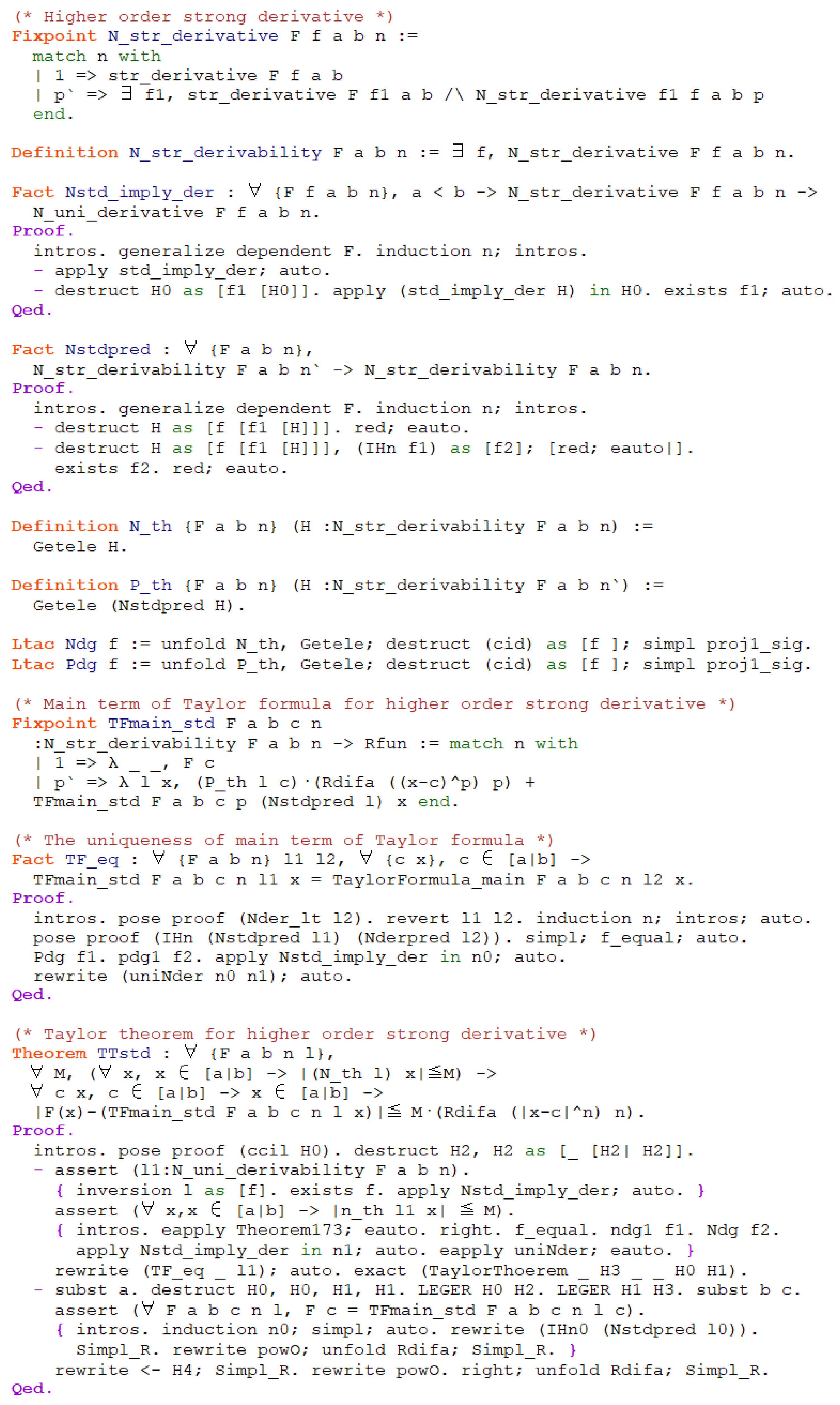
6. Higher Order Derivative

In view of the importance and independent meaning of higher order derivative in calculus, we will focus on it in this section. Specifically, we only consider the higher order form of UnD because it is more applicable than StD. Moreover, some essential contents about higher order strong derivative are shown in Appendix A.

f is the n order derivative of F on $[a,b]$; if $n=1$, then f is the UnD of F on $[a,b]$; otherwise, there exists $f_1$ as the UnD of F on $[a,b]$ and f is the $n-1$ order derivative of $f_1$ on $[a,b]$. Moreover, this is expressed by $F^{\left(n\right)}=f$. If F has the n order derivability, then there exists f as the n order derivative of F on $[a,b]$. Here are the formalizations:

Fixpoint N_uni_derivative F f a b n ≔
          match n with
          | 1 => uni_derivative F f a b
          | p‘ => ∃ f1, uni_derivative F f1 a b /\ N_uni_derivative f1 f a b p
          end.
        Definition N_uni_derivability F a b n ≔ ∃ f, N_uni_derivative F f a b n.
      

We can prove the equivalent definition of higher order derivative.

Fact NderNec : ∀ {F f a b n}, N_uni_derivative F f a b n‘ ->
          ∃ f1, N_uni_derivative F f1 a b n /\ uni_derivative f1 f a b.
        Fact NderSuf : ∀ {F f a b n},
          (∃ f1, N_uni_derivative F f1 a b n /\ uni_derivative f1 f a b) ->
          N_uni_derivative F f a b n‘.
      

Then, we can prove the uniqueness of higher order derivative.

Fact uniNder : ∀ {F f1 f2 a b k},
           N_uni_derivative F f1 a b k -> N_uni_derivative F f2 a b k ->
           ∀ x, x ∈ [a|b] -> f1 x = f2 x.
      

Further, we can prove the following facts by the uniqueness of higher order derivative.

• $F^{\left(n\right)}=f_1$, $f_1^{\left(k\right)}=f_2$, then $F^{(n+k)}=f_2$.
• $F^{\left(n\right)}=f_1$, $F^{(n+k)}=f_2$, then $f_1^{\left(k\right)}=f_2$.

In particular, when $k=1$, these become

• $F^{\left(n\right)}=f_1$, $F^{(n+1)}=f_2$, then $f_2$ is the UnD of $f_1$.
• $F^{\left(n\right)}=f_1$ and $f_2$ is the UnD of $f_1$, then $F^{(n+1)}=f_2$.

The formalizations are as follows:

Fact NderOrdPl : ∀ {F f1 f2 a b n k}, N_uni_derivative F f1 a b n ->
          N_uni_derivative f1 f2 a b k -> N_uni_derivative F f2 a b (Plus_N n k).
        Fact NderOrdMi : ∀ {F f1 f2 a b n k}, N_uni_derivative F f1 a b n ->
          N_uni_derivative F f2 a b (Plus_N n k) -> N_uni_derivative f1 f2 a b k.
        Fact Nderp1 : ∀ {F f1 f2 a b n}, N_uni_derivative F f1 a b n ->
          N_uni_derivative F f2 a b n‘ -> uni_derivative f1 f2 a b.
        Fact Nderp2 : ∀ {F f1 f2 a b n}, N_uni_derivative F f1 a b n ->
          uni_derivative f1 f2 a b -> N_uni_derivative F f2 a b n‘.
      

Like the UnD, higher order derivative has two properties as follows:

Fact Fact_lt : ∀ {F a b k}, N_uni_derivability F a b k -> a < b.
        Fact Nderin : ∀ {F f a b c n},
          c ∈ [a|b] -> c < b -> N_uni_derivative F f a b n -> N_uni_derivative F f c b n.
      

Next, we define four functions ($k=n,k=n-1,k<n,k\le n$) to get the higher order derivative through the n order derivability and the three propositions. They are defined in Coq as follows:

Fact Nderpred : ∀ {F a b n},
          N_uni_derivability F a b n‘ -> N_uni_derivability F a b n.
        Fact Nderltn : ∀ {F a b n k},
          ILT_N k n -> N_uni_derivability F a b n -> N_uni_derivability F a b k.
        Fact Nderlen : ∀ {F a b n m} l,
          N_uni_derivability F a b n -> N_uni_derivability F a b (Minus_N n‘ m (Le_Lt l)).
        Definition n_th {F a b n} (H :N_uni_derivability F a b n) ≔ Getele H.
        Definition p_th {F a b n} (H :N_uni_derivability F a b n‘) ≔ Getele (Nderpred H).
        Definition k_th {F a b n} k (H :ILT_N k n)
          (H0 :N_uni_derivability F a b n) ≔ Getele (Nderltn H H0).
        Definition m_th {F a b n} k (H :ILE_N k n)
          (H0 :N_uni_derivability F a b n) ≔ Getele (Nderlen H H0).
      

We can get the conclusion that if F has the n order derivability, then $F^{\left(k\right)}$ has the $(n-k)$ order derivability where $k<n$.

Fact NderCut : ∀ {F a b n} k l1 (l :N_uni_derivability F a b n),
          N_uni_derivability (k_th k l1 l) a b (Minus_N n k l1).
      

There are several propositions about the higher order derivative operation.

Fact NderfMu : ∀ {F f a b c n}, N_uni_derivative F f a b n ->
          N_uni_derivative (mult_fun c F) (mult_fun c f) a b n.
        Fact NderFPl : ∀ {F f G g a b n},
          N_uni_derivative F f a b n -> N_uni_derivative G g a b n ->
          N_uni_derivative (Plus_Fun F G) (Plus_Fun f g) a b n.
        Fact NderFMi : ∀ {F f G g a b n},
          N_uni_derivative F f a b n -> N_uni_derivative G g a b n ->
          N_uni_derivative (Minus_Fun F G) (Minus_Fun f g) a b n.
        Fact Nderf_mi : ∀ {F f a b n}, N_uni_derivative F f a b n ->
          N_uni_derivative (λ x, F(-x)) (λ x, (-(1))^n · f(-x)) (-b) (-a) n.
      

7. Important Theorems in Calculus

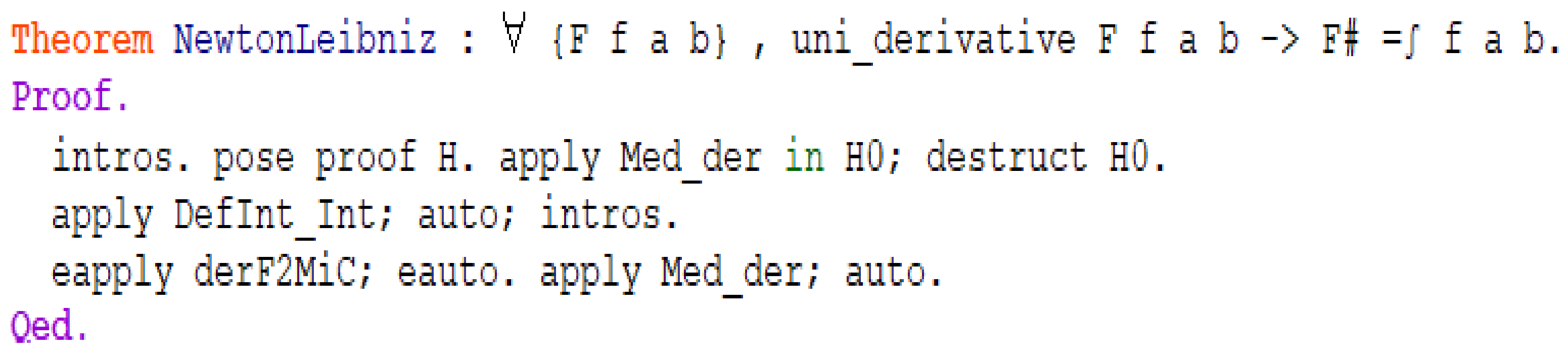
7.1. Newton Leibniz Formula

Let f be the UnD of F, then

$${\int }_a^{b}f\left(x\right)dx=F\left(b\right)-F\left(a\right)$$

The formalization is as follows:

Theorem NewtonLeibniz : ∀ {F f a b} , uni_derivative F f a b -> F# =∫ f a b.
        

Proof. 

Since f is a UnD of F on $[a,b]$, then f is a DCF of F and is uniformly continuous on $[a,b]$. By DefInt_Int, we only need prove that $F\#=G\#$ where G is any function with f as its DCF on $[a,b]$ Since f is the DCF of $F,G$ on $[a,b]$ and f is continuous uniformly on $[a,b]$, then f is UnD of $F,G$. By derF2MiC, the proposition is proved. □

As shown in Figure 1, the formal proof process is very simple.

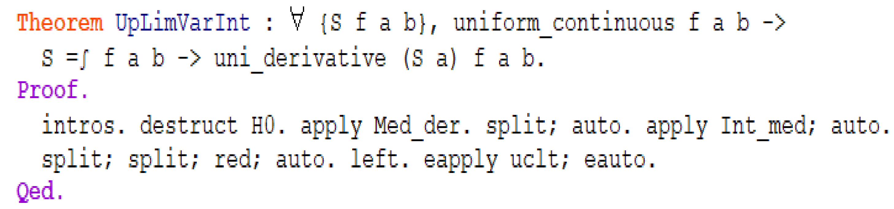
7.2. Upper Limit-Variable Integral

If f is a uniformly continuous function and f has the definite integral on $[a,b]$, and $G\left(x\right):={\int }_a^{x}f\left(t\right)dt$, then f is the UnD of G on $[a,b]$. The formalization is as follows:

Theorem UpLimVarInt : ∀ {S f a b},
            uniform_continuous f a b -> S =∫ f a b -> uni_derivative (S a) f a b.
        

Proof. 

Due to the uniform continuity, we can get $a<b$ then $a\in [a,b]$. By Med_der and Int_med, the proposition is proved. □

As shown in Figure 2, the formal proof process is highly readable in Coq.

7.3. Taylor Formula

The Taylor formula is an important conclusion in calculus, and it has a far-reaching meaning. As it involves much content, we will divide it into four parts to present it.

7.3.1. Taylor Lemma

Let H have the n order derivability on $[a,b]$, if

• $\forall k<n,H^{\left(k\right)}\left(a\right)=0$ and $H\left(a\right)=0$,
• $\forall x\in [a,b],m\le H^{\left(n\right)}\left(x\right)\le M$.

then $\forall x\in [a,b],m\frac{{(x-a)}^n}{n!}\le H\left(x\right)\le M\frac{{(x-a)}^n}{n!}$.

The formalization is as follows:

Theorem TaylorLemma : ∀ {H a b n m M} (l :N_uni_derivability H a b n),
              H a = O -> (∀ k l1, (k_th k l1 l) a = O) ->
              (∀ x, x ∈ [a|b] -> m ≤ (n_th l) x) -> (∀ x, x ∈ [a|b] -> (n_th l) x ≤ M) ->
              ∀ x, x ∈ [a|b] -> m·(Rdifa ((x-a)^n) n) ≤ H x /\ H x ≤ M·(Rdifa ((x-a)^n) n).
          

First, we need to prove a lemma:

$$\forall x\in [a,b],m\frac{{(x-a)}^{k-1}}{(k-1)!}\le H^{(n\prime -k)}\left(x\right)\le M\frac{{(x-a)}^{k-1}}{(k-1)!},1<k\le n$$

The formalization is as follows:

Fact tlp : ∀ {m n} l, ILE_N (Minus_N n‘ m (Le_Lt l)) n.
            Lemma TLpre : ∀ {H a b n m M}
              (l :N_uni_derivability H a b n), (∀ k l1, (k_th k l1 l) a = O) ->
              (∀ x, x ∈ [a|b] -> m ≤ (n_th l) x) -> (∀ x, x ∈ [a|b] -> (n_th l) x ≤ M) ->
              ∀ k l1 l2, let j≔(Minus_N k 1 l2) in  let i≔ (Minus_N n‘ k (Le_Lt l1)) in
              ∀ x, x ∈ [a|b] -> m·(Rdifa ((x-a)^j) j) ≤ (m_th i (tlp l1) l) x /\
              (m_th i (tlp l1) l) x  ≤  M·(Rdifa ((x-a)^j) j).
          

Proof. 

Using the incomplete mathematical induction for k.

When $k=2$, then we prove

$$\forall x\in [a,b],m(x-a)\le H^{(n-1)}\left(x\right)\le M(x-a)$$

Let $f_1\left(x\right):=m(x-a)$ and $f_2\left(x\right):=M(x-a)$. It is obviously seen that $f_1^{\left(1\right)}=m$, $f_2^{\left(1\right)}=M$, and $\forall x\in [a,b],m\le H^{\left(n\right)}\left(x\right)\le M$ from known conditions. Since we have $H^{(n-1)}\left(a\right)=f_1\left(a\right)=f_2\left(a\right)=0$, thus this case is proved by derVle.

Suppose case $k+1$ is true, that is

$$\forall x\in [a,b],m\frac{{(x-a)}^k}{k!}\le H^{(n-k)}\left(x\right)\le M\frac{{(x-a)}^k}{k!}$$

we prove the $k+2$ is true that is

$$\forall x\in [a,b],m\frac{{(x-a)}^{k\prime }}{k\prime !}\le H^{(n-k\prime )}\left(x\right)\le M\frac{{(x-a)}^{k\prime }}{k\prime !}$$

Let $f_1\left(x\right):=m\frac{{(x-a)}^{k\prime }}{k\prime !}$, $f_2\left(x\right):=M\frac{{(x-a)}^{k\prime }}{k\prime !}$ and $F:=H^{(n-k\prime )}$. It is not difficult to prove the propositions: $f_1^{\left(1\right)}=m\frac{{(x-a)}^k}{k!},f_2^{\left(1\right)}=M\frac{{(x-a)}^k}{k!}$, and $F^{\left(1\right)}=H^{(n-k)}$. This case is proved by derVle because $F\left(a\right)=f_1\left(a\right)=f_2\left(a\right)=0$ and the known conditions. □

Next we prove the Taylor Lemma.

Proof. 

When $n=1$. Let $f_1\left(x\right):=m(x-a)$ and $f_2\left(x\right):=M(x-a)$. We can get that $f_1^{\left(1\right)}=m,f_2^{\left(1\right)}=M$, and $\forall x\in [a,b],m\le H^{\left(1\right)}\left(x\right)\le M$. Since $H\left(a\right)=f_1\left(a\right)=f_2\left(a\right)$, thus this case is proved by derVle.

When $n>1$. Let n be the k in TLpre, and we have that

$$m\frac{{(x-a)}^{n-1}}{(n-1)!}\le H^{\left(1\right)}\left(x\right)\le M\frac{{(x-a)}^{n-1}}{(n-1)!}$$

Let $f_1\left(x\right):=m\frac{{(x-a)}^n}{n!}$, $f_2\left(x\right):=M\frac{{(x-a)}^n}{n!}$. Then $f_1^{\left(1\right)}=m\frac{{(x-a)}^{n-1}}{(n-1)}$, $f_2^{\left(1\right)}=M\frac{{(x-a)}^{n-1}}{n-1}$. Since $H\left(a\right)=f_1\left(a\right)=f_2\left(a\right)$, thus this case is proved by derVle. □

7.3.2. Main Term of Taylor Formula

Supposing F has the n order derivability on $[a,b]$,

$$T_{F,c,n}\left(x\right):=F\left(c\right)+\sum _{i=1}^{n-1}\frac{F^{\left(i\right)}\left(c\right){(x-c)}^i}{i!}$$

represents the main term of the n order Taylor formula about F on c, that is, the Taylor formula without remainder.

It is defined in Coq as follows:

Fixpoint TaylorFormula_main F a b c n :N_uni_derivability F a b n -> Rfun ≔
              match n with
              | 1 => λ _ _, F c
              | p‘ => λ l x, (p_th l c)·(Rdifa ((x-c)^p) p) +
                      TaylorFormula_main F a b c p (Nderpred l) x
              end.
          

These two properties can be obtained directly from the expression:

1. $T_{F,c,n}\left(c\right)=F\left(c\right)$;

2. $T_{F,c,n}^{\left(n\right)}=\mathrm{\Phi }\left(0\right),c\in [a,b]$.

Here are the formalizations.

Fact tayp1 : ∀ F a b c n l, TaylorFormula_main F a b c n l c = F c.
            Fact tayp2 : ∀ {F a b c n} l,
              c ∈ [a|b] -> N_uni_derivative (TaylorFormula_main F a b c n l) (ϕ(O)) a b n.
          

7.3.3. Derivative of Main Term of Taylor Formula

Supposing F has the n order derivability on $[a,b]$,

$$D_{F,c,n,k}:=T_{F,c,n}^{\left(k\right)}=\left\{\begin{array}{cc}{T}_{F^{\left(k\right)},c,(n-k)}\hfill & \mathrm{if}k<n\hfill \\ \mathrm{\Phi }\left(0\right)\hfill & \mathrm{if}k\ge n\hfill \end{array}\right.$$

represents the k-th derivative of the main term of the n order Taylor formula about F on c.

It is defined in Coq as follows:

Fact Ndec : ∀ n m, {ILT_N n m} + {ILE_N m n}.
            Definition TFmain_kthd F a b c n k (l :N_uni_derivability F a b n) :Rfun ≔
              match Ndec k n with
              | left l1 =>
                TaylorFormula_main (k_th k l1 l) a b c (Minus_N n k l1) (NderCut k l1 l)
              | right _ => ϕ(O)
              end.
          

These properties can be obtained directly from the expression:

1.$D_{F,c,n\prime ,k}:=\frac{F^{\left(n\right){(x-1)}^{n-1}}}{(n-1)!}+D_{F,c,n,k}$;

2.$D_{F,c,n\prime ,n}:=\mathrm{\Phi }\left(F^{\left(n\right)}\left(c\right)\right)$;

3.$D_{F,c,n,k}\left(c\right):=F^{\left(k\right)}\left(c\right),c\in [a,b]$.

Here are the formalizations.

Fact taykdp1 : ∀ {F a b c k n l} l0, c ∈ [a|b] ->
              let m≔Minus_N n k l0 in (TFmain_kthd F a b c n‘ k l) = Plus_Fun
              (λ x, p_th l c · Rdifa ((x-c)^m) m) (TFmain_kthd F a b c n k (Nderpred l)).
            Fact taykdp2 : ∀ F a b c n l,
              TaylorFormula_kder F a b c n‘ n l = ϕ(n_th (Nderpred l) c).
            Fact taykdp3 : ∀ F a b c n l k l1,
              c ∈ [a|b] -> TaylorFormula_kder F a b c n k l c = k_th k l1 l c.
          

At last, we can verify the correctness of the definition, i.e., $T_{F,c,n}^{\left(k\right)}=D_{F,c,n,k}$.

Fact tayder : ∀ {F a b n} k l c, c ∈ [a|b] -> N_uni_derivative
              (TaylorFormula_main F a b c n l) (TFmain_kthd F a b c n k l) a b k.
          

7.3.4. Taylor Theorem

Let F have the n order derivability on $[a,b]$, and $\forall x\in [a,b],|F^{\left(n\right)}\left(x\right)|\le M$; then for any two points $x,c\in [a,b]$, we have

$$|F\left(x\right)-T_{F,c,n}\left(x\right)|\le M\frac{{(x-c)}^n}{n!}$$

The formalization of this theorem is as follows:

Theorem TaylorThoerem : ∀ {F a b n l},
              ∀ M, (∀ x, x ∈ [a|b] -> |(n_th l) x|≤M) -> ∀ c x, c ∈ [a|b] -> x ∈ [a|b] ->
              |F(x)-(TaylorFormula_main F a b c n l x)|≤ M·(Rdifa (|x-c|^n) n).
          

First, we prove the lemma: If $x\in [c,b]$, the proposition holds. The formalization of the lemma is as follows:

Lemma TTpre : ∀ {F a b n M l},
              (∀ x, x ∈ [a|b] -> |(n_th l) x| ≤ M) -> ∀ c x, c ∈ [a|b] -> x ∈ [c|b] ->
              |F(x)-(TaylorFormula_main F a b c n l x)|≤ M·(Rdifa (|x-c|^n) n).
          

Proof. 

When $c=b$, the left side of the inequality is 0 by tayp1; then this case is proved.

When $c<b$, let $H:=F-T_{F,c,n}$. We can get that H has the n order derivability on $[a,b]$ by tayp2, and further, H also has the n order derivability on $[c,b]$ due to $c<b$. Then, $H\left(c\right)=F\left(c\right)-T_{F,c,n}\left(c\right)=0$ by tayp1. Next, $\forall k<n,H^{\left(k\right)}\left(c\right)=F^{\left(k\right)}\left(c\right)-D_{F,c,n,k}\left(c\right)=0$ by taykdp3. In addition, we have $\forall x\in [c,b],|H^{\left(n\right)}\left(x\right)|\le M$ by tayp2. Therefore, we have $\forall x\in [c,b],H\left(x\right)\le M\frac{{(x-c)}^n}{n!}$ by Taylor Lemma. Because of $|x-c|=x-c$, the lemma is proved. □

Next we prove: If $x\in [a,c]$, the proposition holds on.

Proof. 

If $x\in [a,c]$, then $-x\in [-c,-a],-c\in [-b,-a]$. Let $G\left(x\right):=F(-x)$. We can get that G has the n order derivability on $[-b,-a]$ by Nderf_mi and $\forall x\in [-b,-a],|F^{\left(n\right)}(-x)|\le M$. By the first case, we have

$$\forall x\in [-c,-a],|G\left(x\right)-T_{G,-c,n}\left(x\right)|\le M\frac{{|x-(-c)|}^n}{n!}$$

$$\downarrow u=-x$$

$$\forall u\in [a,c],|F\left(u\right)-T_{G,-c,n}(-u)|\le M\frac{{|u-c|}^n}{n!}$$

As long as $T_{G,-c,n}(-u)=T_{F,c,n}\left(u\right)$, this case is proved.

$$T_{G,-c,n}(-u)=G(-c)+\sum _{i=1}^{n-1}\frac{G^{\left(i\right)}(-c){(-u-(-c))}^i}{i!}$$

$$=F\left(c\right)+\sum _{i=1}^{n-1}\frac{{(-1)}^i{F}^{\left(i\right)}\left(c\right){(-1)}^i{(u-c)}^i}{i!}=T_{F,c,n}\left(u\right)$$

So the proposition is proved. We can deduce that the Taylor formula for strong derivative also holds; the details can be found in the appendix. □

8. Conclusions and Future Work

The calculus without limit theory starts from the physical facts. Then, the concept of the difference-quotient control function is introduced, which corresponds to but is not equivalent to the mean value theorem in traditional calculus. The conclusions drawn from it are amazing, but it is not necessarily the derivative. On the one hand, it can become a strong derivative with a Lipschitz function, which is enough for practical application in the field of science and engineering. On the other hand, it can become a uniform derivative with a uniformly continuous function to relax the too restrictive condition of a Lipschitz function. Both of them have all the properties of a difference-quotient control function and have uniqueness and can carry out binary operations. Furthermore, the integral system and definite integral are naturally defined by axiomatization and are closely related to the difference-quotient control function. With these basic concepts, some important theorems in calculus can be proved. Compared with derivative in the generic sense, the strong derivative also satisfies that the derivative is a Lipschitz function and the uniform derivative also satisfies that the derivative is continuous. In summary, the condition of the derivative in this theory is indeed stronger than that of the traditional derivative, but there is no difference in practical application.

We are formalizing the calculus without limit theory on the basis of a system without real number completeness. It is feasible and rigorous to verify this theory by the proof assistant Coq. Moreover, we obtain some facts which are not pointed out in previously developed paper proofs. Uniform derivability only holds on a strict interval. To prove the strong derivability, we only need to consider whether it holds on a strict interval. So strong derivability implies uniform derivability only on a strict interval. The complete source files containing the Coq formalization and proofs are accessible at:

https://github.com/coderfys/Analysis/tree/main/Calculus_without_limt, accessed on 10 June 2021

In the future, we will complete the formalization of deeper contents of this theory. At the same time, this theory can also be applied to calculus teaching. Furthermore, we can supplement the real number completeness to enrich the theory and unify it with traditional calculus in a formal way.

References

1. Bertot, Y.; Castéran, P. Interactive Theorem Proving and Program Development. Coq’Art: The Calculus of Inductive Constructions; Texts in Theoretical Computer Science; Springer: Berlin/Heidelberg, Germany, 2004. [Google Scholar]
2. Chlipala, A. Certified Programming with Dependent Types: A Pragmatic Introduction to the Coq Proof Assistant; MIT Press: Cambridge, MA, USA, 2013. [Google Scholar]
3. The Coq Development Team. The Coq Proof Assistant Reference Manual (Version 8.9.1). 2019. Available online: https://coq.inria.fr/distrib/8.9.1/refman/ (accessed on 4 August 2019).
4. Nipow, T.; Paulson, L.; Wenzel, M. Isabelle/HOL: A Proof Assistant for Higher-Order Logic; Springer: Berlin/Heidelberg, Germany, 2002. [Google Scholar]
5. Harrision, J. The HOL Light Theorem Prover. 2020. Available online: http://www.cl.cam.ac.uk/~jrh13/hol-light/ (accessed on 18 May 2018).
6. Beeson, M. Mixing computations and proofs. J. Formaliz. Reason. 2016, 9, 71–99. [Google Scholar]
7. Hales, T. Formal proof. Not. Am. Math. Soc. 2008, 55, 1370–1380. [Google Scholar]
8. Harrision, J. Formal proof—Theory and practice. Not. Am. Math. Soc. 2008, 55, 1395–1406. [Google Scholar]
9. Wiedijk, F. Formal proof—Getting started. Not. Am. Math. Soc. 2008, 55, 1408–1414. [Google Scholar]
10. Cruz-Filipe, L.; Marques-Silva, J.; Schneider-Kamp, P. Formally verifying the solution to the Boolean Pythagorean triples problem. J. Autom. Reason. 2019, 63, 695–722. [Google Scholar] [CrossRef]
11. Gonthier, G. Formal proof—The Four Color Theorem. Not. Am. Math. Soc. 2008, 55, 1382–1393. [Google Scholar]
12. Gonthier, G.; Asperti, A.; Avigad, J.; Bertot, Y.; Cohen, C.; Garillot, F.; Roux, S.L.; Mahboubi, A.; O’Connor, R.; Biha, S.O.; et al. Machine-checked proof of the Odd Order Theorem. In Lecture Notes in Computer Science, Proceedings of the Interactive Theorem Proving 2013 (ITP 2013), Rennes, France, 22–26 July 2013; Blazy, S., Paulin-Mohring, C., Pichardie, D., Eds.; Springer: Berlin/Heidelberg, Germany, 2013; Volume 7998, pp. 163–179. [Google Scholar]
13. Hales, T.; Adams, M.; Bauer, G.; Dang, T.D. A Formal Proof of the Kepler Conjecture. Forum of Mathematics, Pi; Cambridge University Press: Cambridge, UK, 2017; Volume 5, pp. 1–29. [Google Scholar]
14. Hales, T. A proof of the Kepler conjecture. Ann. Math. 2005, 162, 1065–1183. [Google Scholar] [CrossRef] [Green Version]
15. Heule, M.; Kullmann, O.; Marek, V. Solving and Verifying the Boolean Pythagorean Triples Problem via Cube-and-Conquer. In Lecture Notes in Computer Science, Proceedings of the Theory and Applications of Satisfiability Testing 2016(SAT 2016), Bordeaux, France, 5–8 July 2016; Creignou, N., Le Berre, D., Eds.; Springer: Cham, Switzerland, 2016; Volume 9710, pp. 228–245. [Google Scholar]
16. Vivant, C. Thèoréme Vivamt; Grasset: Prais, France, 2012. [Google Scholar]
17. Voevodsky, V. Univalent Foundations of Mathematics; Beklemishev, L., De Queiroz, R., Eds.; Springer: Berlin/Heidelberg, Germany, 2011; Volume 6642, p. 4. [Google Scholar]
18. Katz, V. A History of Mathematics: An Introduction; Pearson Addison-Wesley: Boston, MA, USA, 2009. [Google Scholar]
19. Grabiner, J.V. Who gave you the epsilon? Cauchy and the origins of rigorous calculus. Am. Math. Mon. 1983, 90, 185–194. [Google Scholar] [CrossRef]
20. Rusnock, P.; Kerr-Lawson, A. Bolzano and uniform continuity. Hist. Math. 2005, 32, 303–311. [Google Scholar] [CrossRef] [Green Version]
21. Courant, R.; Robbins, H.; Stewart, I. What Is Mathematics? An Elementary Approach to Ideas and Methods; Oxford University Press: Oxford, UK, 1996. [Google Scholar]
22. Dovermann, K.H. Applied Calculus. 1999. Available online: https://math.hawaii.edu/~heiner/calculus.pdf (accessed on 20 December 2019).
23. Lin, Q. Free Calculus: A Liberation from Concepts and Proofs; World Scientific: Singapore, 2008. [Google Scholar]
24. Livshits, M. Simplifying Calculus by Using Uniform Estimates. 2004. Available online: https://www.mathfoolery.com/talk-2004.pdf (accessed on 15 March 2020).
25. Lusternik, L.A.; Sobolev, V.J. Elements of Functional Analysis, 3rd ed.; John Wiley & Sons: New York, NY, USA, 1975. [Google Scholar]
26. Sparks, J.C. Calculus without Limits-Almost; AuthorHouse: Bloomington, IN, USA, 2005. [Google Scholar]
27. Zhang, J. Let calculus more elementary. J. Cent. China Norm. Univ. (Nat. Sci.) 2006, 45, 475–484. [Google Scholar]
28. Lin, Q. Fast Calculus; Science Press: Beijing, China, 2009. [Google Scholar]
29. Zhang, J. Straightforward Calculus; Science Press: Beijing, China, 2010. [Google Scholar]
30. Zhang, J.; Tong, Z. Calculus without Limit Theory. 2018. Available online: https://arxiv.org/abs/1802.03029 (accessed on 10 September 2020).
31. Lin, Q.; Zhang, J. What Can Be Done Prior to Calculus. Stud. Coll. Math. 2019, 22, 1–15. [Google Scholar]
32. Lin, Q.; Zhang, J. Calculus prior to limits. Stud. Coll. Math. 2020, 23, 1–16. [Google Scholar]
33. Lin, Q.; Tong, Z.; Zhang, J. Introducing continuity in calculus before limits. Stud. Coll. Math. 2020, 23, 1–10. [Google Scholar]
34. Landau, E. Foundations of Analysis: The Arithmetic of Whole, Rational, Irrational, and Complex Numbers; Chelsea Publishing Company: New York, NY, USA, 1966. [Google Scholar]
35. Fu, Y.; Yu, W. A Formalization of Properties of Continuous Functions on Closed Intervals. In Lecture Notes in Computer Science, Proceedings of the International Congress on Mathematical Software (ICMS 2020), Braunschweig, Germany, 13–16 July 2020; Bigatti, A., Carette, J., Joswig, M., de Wolff, T., Eds.; Springer: Cham, Switzerland, 2020; Volume 12097, pp. 272–280. [Google Scholar]
36. Fu, Y.; Yu, W. Formalization of the Equivalence among Completeness Theorems of Real Number in Coq. Mathematics 2021, 9, 38. [Google Scholar] [CrossRef]
37. Livshits, M. You Could Simplify Calculus. 2009. Available online: https://arxiv.org/abs/0905.3611 (accessed on 15 March 2020).
38. Zhang, J. Axiomatic method for the definition of definite integral. J. Guangzhou Univ. 2007, 6, 1–5. [Google Scholar]
39. Zhang, J.; Feng, Y. A new way viewing the foundation of calculus. Sci. China Ser. A 2009, 39, 247–256. [Google Scholar]
40. Zhang, J.; Feng, Y. The third generation calculus. Chin. J. Nat. 2010, 32, 67–71. [Google Scholar]
41. Van Benthem Jutting, L.S. Checking Landau’s “Grundlagen” in the AUTOMATH System. Ph.D. Thesis, Eindhoven University of Technology, Eindhoven, The Netherlands, 1977. [Google Scholar]
42. Brown, C.E. Faithful Reproductions of the Automath Landau Formalization. Technical Report. 2011. Available online: https://www.ps.uni-saarland.de/Publications/documents/Brown2011b.pdf (accessed on 28 July 2018).
43. Guidi, F. Verified Representations of Landau’s “Grundlagen” in the lambda-delta Family and in the Calculus of Constructions. J. Formaliz. Reason. 2016, 8, 93–116. [Google Scholar]
44. Cruz-Filipe, L. A Constructive Formalization of the Fundamental Theorem of Calculus. In Lecture Notes in Computer Science, Proceedings of the International Workshop on Types for Proofs and Programs (TYPES 2002), Bergen Dal, The Netherlands, 24–28 April 2002; Springer: Berlin/Heidelberg, Germany, 2002; Volume 2646, pp. 108–126. [Google Scholar]
45. Cruz-Filipe, L.; Geuvers, H.; Wiedijk, F. C-CoRN, the Constructive Coq Repository at Nijmegen. In Lecture Notes in Computer Science, Proceedings of the International Conference on Mathematical Knowledge Management (MKM 2004), Białowieża, Poland, 19–21 September 2004; Springer: Berlin/Heidelberg, Germany, 2004; Volume 3119, pp. 88–103. [Google Scholar]
46. Boldo, S.; Lelay, C.; Melquiond, G. Coquelicot: A User-Friendly Library of Real Analysis. Math. Comput. Sci. 2015, 9, 41–62. [Google Scholar] [CrossRef] [Green Version]
47. Guo, L.; Fu, Y.; Yu, W. A Mechanized Proof System of The Third Generation Calculus in Coq. Sci. China Ser. A 2021, 51, 115–136. [Google Scholar]
48. Coquand, T.; Paulin, C. Inductively Defined Types. In Lecture Notes in Computer Science, Proceedings of the International Conference on Computer Logic (COLOG 1988), 12–16 December 1988; Springer: Berlin/Heidelberg, Germany, 1990; Volume 417, pp. 50–66. [Google Scholar]
49. Coquand, T.; Huet, G. The calculus of constructions. Inf. Comput. 1988, 76, 95–120. [Google Scholar] [CrossRef] [Green Version]
50. Luo, Z. ECC, an extended calculus of constructions. In Proceedings of the Fourth Annual Symposium on Logic in Computer Science, Pacific Grove, CA, USA, 5–8 June 1989; IEEE Press: Piscataway, NJ, USA, 1989; pp. 386–395. [Google Scholar]
51. Boulier, S.; Pédrot, P.; Tabareau, N. The next 700 syntactical models of type theory. In Proceedings of the 6th ACM SIGPLAN Conference on Certified Programs and Proofs, Paris, France, 16–17 January 2017; ACM: New York, NY, USA, 2017; pp. 182–194. [Google Scholar]
52. Yu, W.; Sun, T.; Fu, Y. Machine Proof System of Axiomatic Set Theory; Science Press: Beijing, China, 2020. [Google Scholar]
Figure 1. The formalization of Newton Leibniz formula.
Mathematics 09 01377 g001
Figure 2. The formalization of differentiability of upper limit-variable integral.
Mathematics 09 01377 g002