1. Introduction
In the fields of advanced equipment manufacturing for example aerospace and new energy, hard and brittle materials such as beryllium, fused silica, and diamond are widely used to manufacture products and devices. Generally, when machining (drilling or cutting) brittle and hard materials, it is pretty easy to cause damage on the processed material. Therefore, at present, laser is commonly used to irradiate the surface of the processed material, after which the processed materials obtain heat through the interaction between light and itself, and the processing quality is significantly improved by heating and modification. In order to find the optimal laser intensity and distribution, it is necessary to calculate the propagation state of light and heat in three-dimensional object. Common numerical methods are the finite element method (FEM) and the finite difference method (FDM) [
1,
2], but they all require large amounts of computation.
For the purpose, some numerical methods had been proposed [
3,
4,
5,
6,
7,
8,
9,
10,
11,
12,
13,
14], such as the alternating direction implicit (ADI) finite-difference time-domain method (FDTD) and its convolution perfect matching layer (CPML). The implementation of the ADI-FDTD and its CPML is divided into three steps. Firstly, transform the finite difference time domain method in the traditional three-dimensional cylindrical coordinate system into a matrix expression. Secondly, matrix expression of ADI-FDTD method in three-dimensional cylindrical coordinate system is proposed by matrix transformation. Finally, the influence parameters of the marching layer are added to the method in the form of auxiliary variables.
The existing methods directly give a three-dimensional cylindrical coordinate model in the electromagnetic environment, combined with the unconditionally stable ADI algorithm. However, we propose a three-dimensional heat conduction model of laser processing in the rectangular coordinate system, which is then discretely transformed, simplified, and solved in three steps. Firstly, a three-dimensional heat conduction model in a rectangular coordinate system is developed, and it is transformed into a three-dimensional heat conduction model in the cylindrical coordinate system. Secondly, since the heat conduction discussed in this article is irrelevant with the angle in the cylindrical coordinate system, the three-dimensional problem in cylindrical coordinates is simplified to a two-dimensional problem. Finally, we use the backward Euler method and Crank–Nicolson method, combined with the unconditionally stable ADI method for discretization.
In order to solve this problem, we first develop the heat conduction equation and boundary conditions. According to the characteristics of laser beam, the heat conduction equation solving problem in three-dimensional rectangular coordinate system is transformed into the heat conduction equation solving problem in two-dimensional cylindrical coordinate system by using cylindrical coordinate transformation. Finally, an alternate implicit scheme algorithm is constructed. In conclusion, the heat conduction distribution can be solved quickly and stably, which provides an effective calculation method for the optimization of related parameter.
2. Mathematical Model
The problem model discussed in this article is first proposed in a rectangular coordinate system, and then converted to a corresponding cylindrical coordinate system for discretization and solution. The significance of this chapter is to give the origin of the cylindrical coordinate equation model in the article and connect it to the original equation model in the rectangular coordinate system.
Suppose
is a cylinder with the origin of the coordinates as the center, then the model of the problem for three-dimensional heat conduction is as follows:
where
.
Boundary value conditions of the first kind are:
Boundary value conditions of the third kind are:
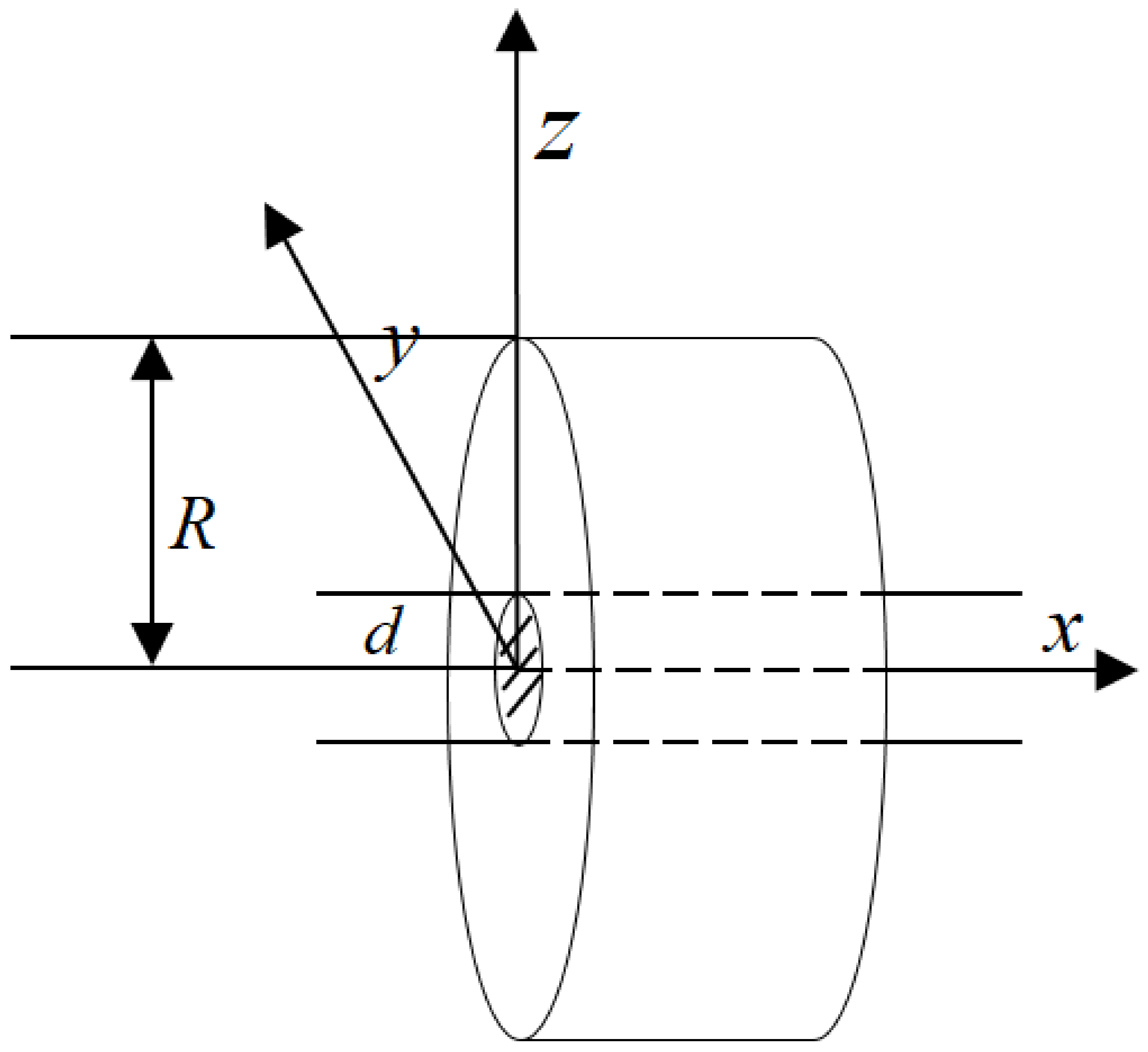
where
is the laser irradiation area,
is the laser radius,
is the material’s absorption rate of laser energy,
is the heat dissipation coefficient, and
is the initial environmental temperature, as shown in
Figure 1.
Consider the problem model under the column coordinates and make the following coordinate transformation:
Then, Equation (1) is transformed into the following form:
where
.
When the temperature distribution
is independent of the
, Equation (6) is transformed into the simpler form:
Transforming Equation (1) into Equation (7) is equivalent to transforming three-dimensional problems into two-dimensional problems. Compared with the direct solution of three-dimensional problems, we have simplified the problem, saved time, and improved the efficiency.
Consider the transformed two-dimensional problem model as follows:
Boundary value conditions of the first kind are as follows:
Boundary value conditions of the third kind are as follows:
The alternate direction implicit format (abbreviated as ADI format) is an unconditionally stable format which can be solved by the catch-up method. This method is also called the P-R method, which was proposed by Peaceman and Rachford in 1955, and will be used to calculate the matrix form under the column coordinate.
3. Establishment of Differential Approximation
In the case of , the space step is set to be and the time step is set to be Where and are positive integers, we have , , and So we get a grid subdivision of the interval, and is a node.
3.1. Difference Scheme for the Backward Euler Method
At node
, Equation (8) is considered as:
Using the backward Euler method to discretize Equation (12), we obtain [
2]:
where the total truncation error is as follow:
The difference equation can be obtained by replacing the exact solution
with an approximate numerical solution
and discarding the truncation error
:
3.2. Difference Scheme for Crank–Nicolson Method
Let
, and at node
, homogeneous form of Equation (8) is considered as the following form:
Using Crank–Nicolson method to discretize Equation (16), we obtain [
2]:
where the total truncation error is:
The difference equation is obtained by replacing the exact solution
with a numerical solution
and discarding the truncation error
:
3.3. Difference Scheme for the First Kind of Boundary Value
3.3.1. Difference Scheme for ADI with the Backward Euler Method
The difference scheme can be obtained by synthesizing the initial value condition and the boundary value condition as follows:
The difference equation is written as:
There exists a normal number
independent of
and
that causes the total truncation error:
In Equation (23), adding the minor term
leads to:
To facilitate the calculation, the transition layer variable
is introduced, and the above equation becomes:
Denote
and
then the vector form of the above two equations is:
Denote
then we have:
Denote
then we have:
The transition layer variable
should satisfy:
There exists a normal number
, independent of
and
, so that the minor term is:
Therefore, Equations (24) and (38), show that a normal number
is independent of
and
, so the total error
of difference schemes for ADI with the backward Euler method of the first kind of boundary value is:
3.3.2. Difference Scheme for ADI with Crank–Nicolson Method
The difference scheme is obtained by synthesizing the initial value condition and the boundary value condition:
The difference equation is written as:
There exists a normal number
independent of
and
that causes the total truncation error:
In Equation (43), adding the minor term
leads to:
To facilitate the calculation, the transition layer variable
is introduced, and the above equation becomes:
Denote
, then the vector forms of the above two equations are as follows:
Denote
then we derive following forms:
Denote
then we get:
The transition layer variable
should satisfy:
There exists a normal number
, independent of
and
, so the minor term is:
Therefore, Equations (44) and (56), demonstrate that the normal number
is independent of
and
, so the total error
of difference schemes for ADI with Crank–Nicolson method of the first kind of boundary value is:
3.4. Difference Scheme for the Third Kind of Boundary Value
3.4.1. Difference Scheme for ADI with the Backward Euler Method
Based on the initial value condition, the boundary value condition and Equation (25), the difference scheme is obtained:
It is the same as the difference scheme under the boundary values of the first kind, and finally discretized into the corresponding ADI scheme. Therefore, the rest are consistent, except that boundary value of the third type enjoys a separate center discretization, and that the approaches to process discrete ADI scheme for and in the inner point vary widely. Therefore, only the discretization of the third type of boundary value and the processing mode of the discrete ADI format when and are discussed.
According to Equation (39), the total error
of the internal point is:
For
, it is discretized as the center at
,
where
is the virtual symmetric point of
about
, and is estimated to be [
3]:
According to Equations (62) and (63), we obtain:
For
, it is discretized as the center at
,
where
is the virtual symmetric point of
about
, and is estimated to be [
3]:
According to Equations (64)–(66), we have:
For
, it is discretized as the center at
,
where
is the virtual symmetric point of
about
, and is estimated to be [
3]:
According to Equations (67)–(69), we have:
For
, it is discretized as the center at
,
where
is the virtual symmetric point of
about
, and is estimated to be [
3]:
According to Equations (70) and (71), we have:
If
, the vector form of ADI with the backward Euler format is:
The third kind of boundary discrete
are substituted into the above two equations to obtain the final discrete format for
. The processing method for
performs the same as the one when
. Therefore, the final matrix form of the difference scheme for the third kind of boundary value is:
where,
The other matrices, , and are the same as the case of the first kind of boundary value.
The discretization of the third kind of boundary value is all the central difference quotient discretization, so there exists a normal number
independent of
and
, so that the total error
of boundary value discretization be:
Therefore, Equations (61) and (78) represent that the normal number
is independent of
and
, so the total error
of difference schemes for ADI with the backward Euler method of the third kind of boundary value is:
3.4.2. Difference Scheme for ADI with Crank–Nicolson Method
Based on the initial value condition, the boundary value condition and Equation (45), the difference scheme is obtained:
The discrete processing of interior points and boundary values is the same as that of ADI with the backward Euler method for the third kind of boundary value. Therefore, the final matrix form of the difference scheme for the third kind of boundary value is:
where,
The other matrices, , and are the same as the case of the first kind of boundary value.
Therefore, Equations (57) and (78) show that the normal number
is independent of
and
, so the total error
of difference schemes for ADI with Crank–Nicolson method of the third kind of boundary value is:
4. Stability and Convergence of Difference Scheme Solutions
4.1. Stability of Difference Scheme Solutions
The following will prove that ADI format with the backward Euler method and ADI format with Crank–Nicolson method are unconditionally stable whether for the first kind of boundary value or the third kind of boundary value.
Definition 1. A functionis defined on. Ifthen there exists:where is an imaginary unit and the above transformation is called the Fourier transform.
Definition 2. Themodule refers to the Euclidean module, and thestable refers to the stability under the second norm [2]. Theorem 1. The difference Equation (25) under the first kind of the boundary value and the boundary value of the third kind is unconditionallystable.
Proof. From the total error of the differential format for the first kind of boundary value and the total error of the differential format for the third kind of boundary value, the total error is . □
Let
be the grid ratio and use the Fourier method to analyze the stability of Equation (25):
Since the stability of homogeneous equations and non-homogeneous equations are consistent, the stability of homogeneous equations can be discussed. The difference equation of ADI with the backward Euler method corresponding to the homogeneous equation is:
Substituting
and
into the Equation (90), we get
where the growth factor
is represented as:
then,
where
. Obviously,
means that the difference scheme Equation (90) is unconditionally
stable. Therefore, the difference Equation (25) is unconditionally
stable.
Theorem 2. The difference Equation (45) for the first kind of the boundary value and the third kind of boundary value is unconditionallystable.
Proof. From the total error of the differential format for the first kind of the boundary value and the total error of the differential format for the third kind of the boundary value, the total error is . □
Let
be the grid ratio and use the Fourier method to analyze the stability of Equation (45):
Substituting
and
into Equation (45), we get
where the growth factor
of Equation (45) is as the following form:
then,
where
. Obviously,
means that the difference scheme Equation (45) is unconditionally
stable.
4.2. Convergence of Difference Scheme Solutions
The following will prove that ADI format with the backward Euler method and ADI format with Crank–Nicolson method are convergent whether for the first kind of boundary value or the third kind of boundary value.
Definition 3. For a sufficiently smooth function, if the time step and the space step both approach 0, the truncation error of the difference equation approaches 0 for each node, it is said that the difference equation approximates the differential equation, that is, the difference equation is consistent with differential equations [2]. Theorem 3. If the difference equation satisfies the consistency condition and is stable according to the initial value, the difference solution converges to the solution of the original equation [2]. Theorem 4. The difference Equation (25) in the case of boundary value of the first kind and boundary value of the third kind is consistent.
Proof. The consistency of the difference equation can be proved by the Taylor expansion method. □
For the difference scheme Equation (25):
is expanded at node
for
,
and
are expanded at node
and
for
, respectively,
and
are expanded at node
and
for
, respectively. We have obtained:
In the above equation, when , all the terms at the right-hand side of the above equation are close to 0, and the difference equation approaches to the original differential equation. Therefore, the difference Equation (25) is consistent with the original equation.
Theorem 5. The difference Equation (25) in the case of boundary value of the first kind and the third kind of boundary value is convergent.
Proof. Order error is , and according to Theorems 3, 4, and 1, the difference scheme Equation (25) in the case of boundary value of the first kind and the third kind of boundary value is convergent. □
Theorem 6. The difference scheme Equation (45) in the case of the first kind of boundary value and the third kind of boundary value is consistent.
Proof. The consistency of the difference equation can be proved by the Taylor expansion method. □
For the difference Equation (45):
and
is expanded at node
for
,
and
are expanded at node
and
for
, respectively,
and
are expanded at node
and
for
, respectively. We have obtained:
In the above equation, when , all the terms at the right-hand side of the above equation are close to 0, and the difference equation approaches to the original differential equation. Therefore, the difference Equation (45) is consistent with the original equation.
Theorem 7. The difference Equation (45) in the case of the first kind of boundary value and the third kind of boundary value is convergent.
Proof. Order error is , and according to theorems 3, 6, and 2, the difference scheme Equation (45) in the case of the first kind of boundary value and the third kind of boundary value is convergent. □
5. Examples
5.1. Verification of Convergence of Algorithm
5.1.1. Example of ADI with the Backward Euler Method
Using the difference scheme for ADI with the backward Euler method of the first kind of boundary value to solve the following definite solution problems, we can verify the convergence of the algorithm.
Example 1. the exact solution of the above fixed solution problem is .
Space interval is uniformly divided into blocks. Denote , , , Time interval is uniformly divided into blocks. Denote , and call as a network node.
The calculation formula of the maximum error
of the numerical solution is given by:
The absolute error is the absolute value of the distinction between the exact solution and numerical solution.
Table 1 shows the numerical solution, the exact solution, and the absolute error at some nodes when
and
.
Table 2 shows the maximum error of the numerical solution when the asynchronous step length is taken. It performs that when the space step is reduced to 1/2 and the time step is reduced to 1/4, the maximum error is approximately reduced by about 3/4.
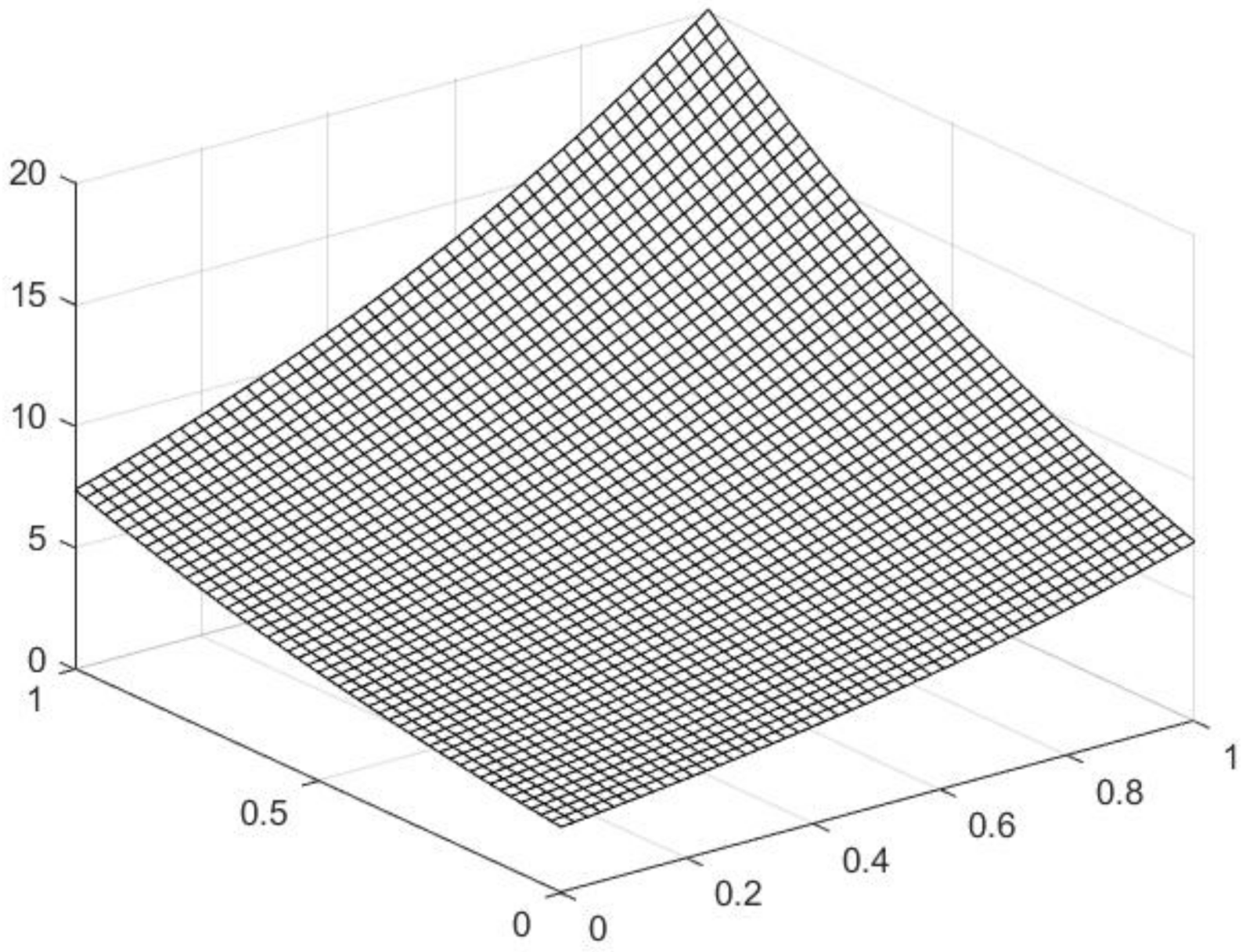
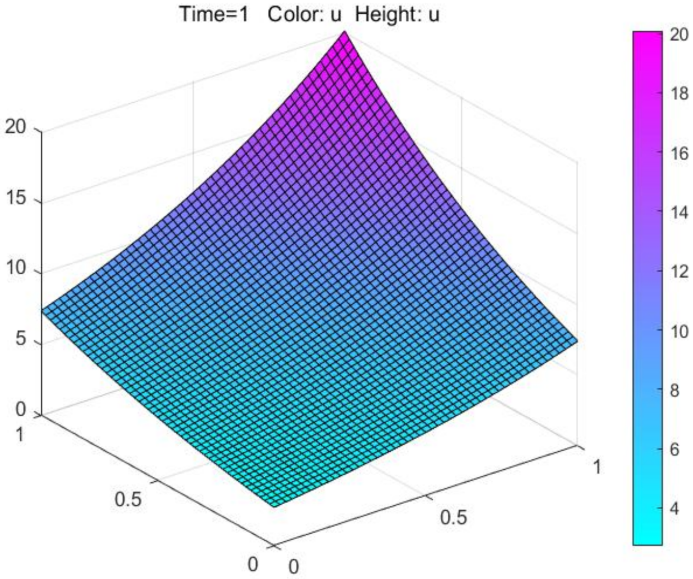
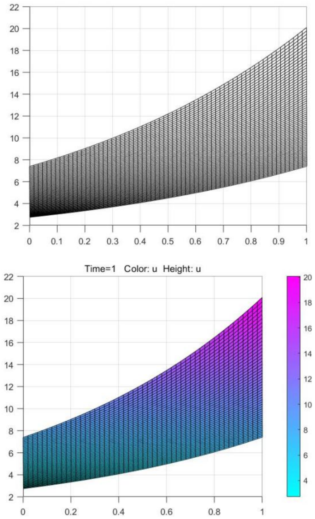
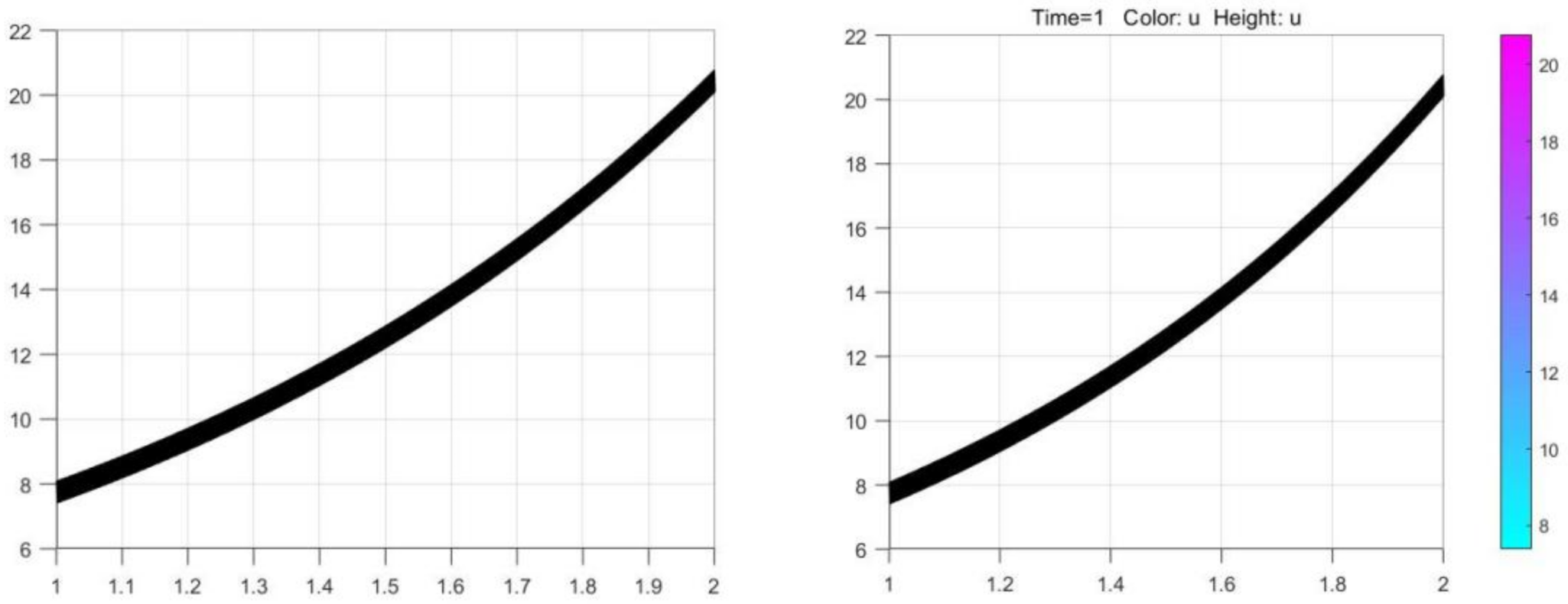
Figure 2 shows the three-dimensional image of the approximate solution of the difference equation when
and
.
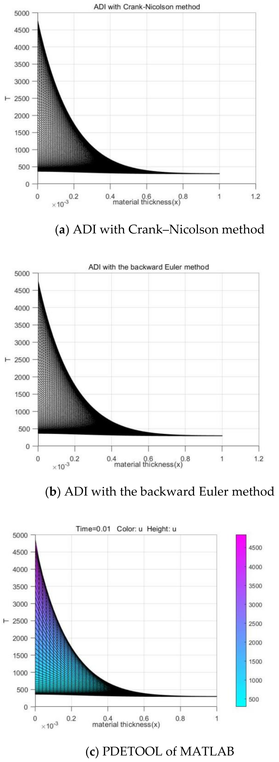
Figure 3 shows the numerical solutions obtained by PDETOOL of MATLAB.
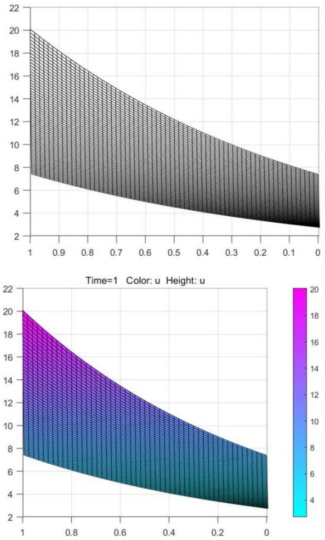
Compare the longitudinal section and the cross section of
Figure 2 and
Figure 3. If the similarity is high, it means that the numerical solution obtained by the algorithm is basically consistent with the numerical solution given by PDETOOL of MATLAB. It shows that the algorithm is more accurate.
It shows from
Figure 2,
Figure 3,
Figure 4 and
Figure 5 that the numerical solution obtained by the ADI with the backward Euler method for the first kind of boundary value is in good agreement with the numerical solution given by the PDETOOL of MATLAB in the same environment.
5.1.2. Example of ADI with Crank–Nicolson Method
Using the difference scheme for ADI with Crank–Nicolson method of the first kind of boundary value to solve the following definite solution problems, we verify the convergence of the algorithm.
Example 2. the exact solution of the above fixed solution problem is .
Space interval is uniformly divided into blocks. Denote , , , Time interval is uniformly divided into blocks. Denote , and call as a network node.
The calculation formula of the maximum error
of the numerical solution is given by:
Table 3 shows the numerical solution, the exact solution, and the absolute error at some nodes when
and
.
Table 4 shows the maximum error of the numerical solution when the asynchronous step length is taken. It represents that when the space step is reduced to 1/2 and the time step is decreased to 1/2, the maximum error is approximately dropped to about 3/4.
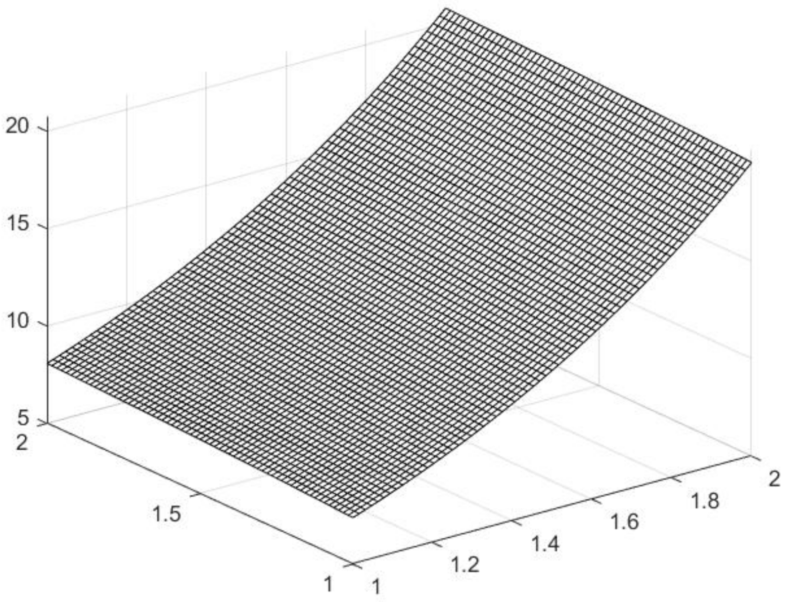
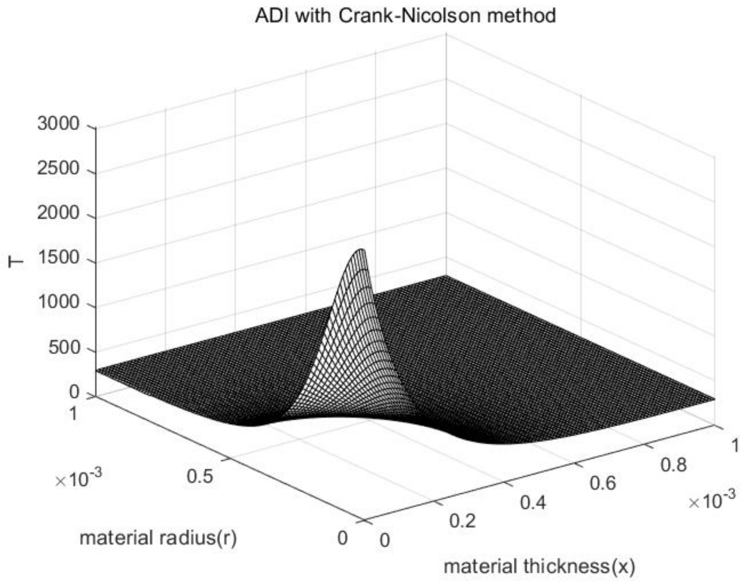
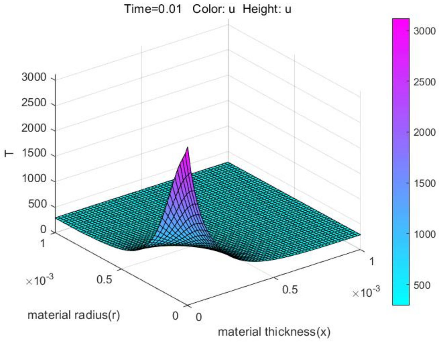
Figure 6 shows the three-dimensional image of the approximate solution of the difference equation when
and
.
Figure 7 shows the numerical solutions obtained by PDETOOL of MATLAB.
Compare the longitudinal section and the cross section of
Figure 6 and
Figure 7. If the comparison is highly similar, the numerical solution obtained by the algorithm is basically consistent with the numerical solution given by PDETOOL of MATLAB, which shows that the algorithm is much accurate.
From
Figure 6,
Figure 7,
Figure 8 and
Figure 9, the numerical solution obtained by the ADI with Crank–Nicolson method for the first kind of boundary value is in good agreement with the numerical solution given by the PDETOOL of MATLAB in the same environment.
5.2. Laser Machining Simulation
We now use the difference scheme of the third kind of boundary value to solve the laser machining problem.
Example 3. Let a laser beam irradiate the surface of the material vertically under the ambient temperature of
. For simplicity, we consider that the input of laser energy acts on the material surface in the form of Gaussian heat flux. In this way, the center of the laser can reach the heat peak, and the temperature of the material boundary tends to the initial temperature. Therefore, the laser radius is equal to the material radius.
Table 5 shows the thermal property parameters of 316 stainless steel.
The input of laser energy acts on the material surface in the form of Gaussian heat flux, specifically:
In the laser irradiation area
, the moving laser beam is loaded through the boundary conditions of the surface heat source:
The boundary outside the laser irradiation area
is in contact with air, and the boundary conditions are as following:
The initial temperature of the substrate is the ambient temperature, that is, the initial conditions of the substrate are:
Cylindrical coordinates should be adopted to this three-dimensional problem. Since the temperature distribution along the depth is symmetric after the laser beam irradiates the surface of the material, it can be converted into a two-dimensional problem with coordinates
. The heat conduction format in cylindrical coordinates is rewritten as:
where
is the thermal diffusivity.
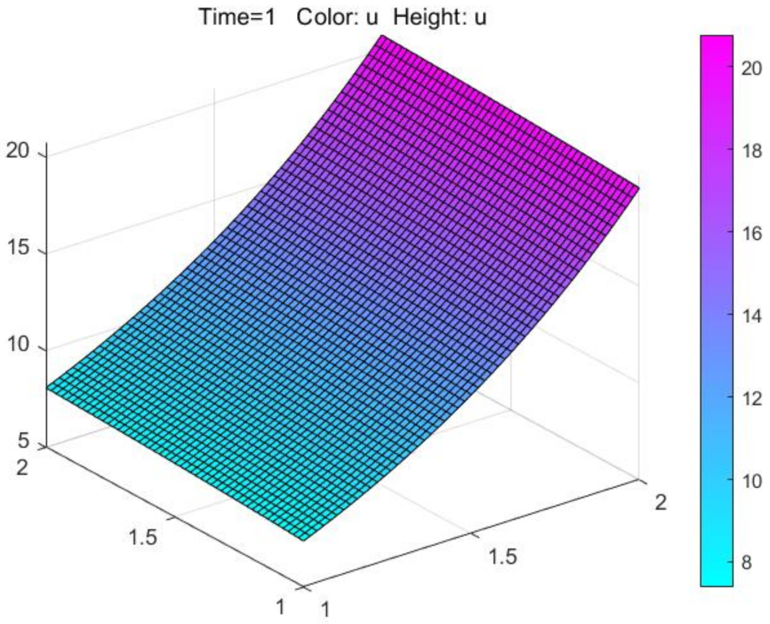
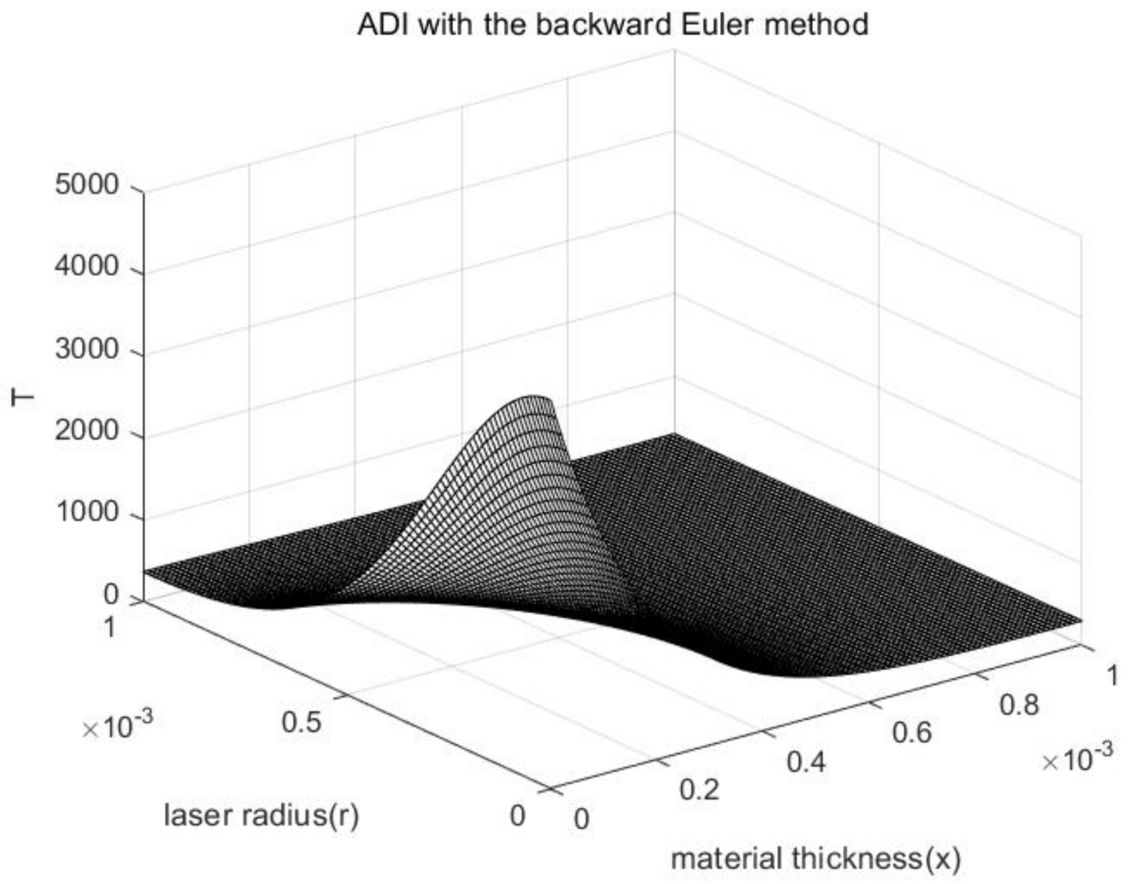
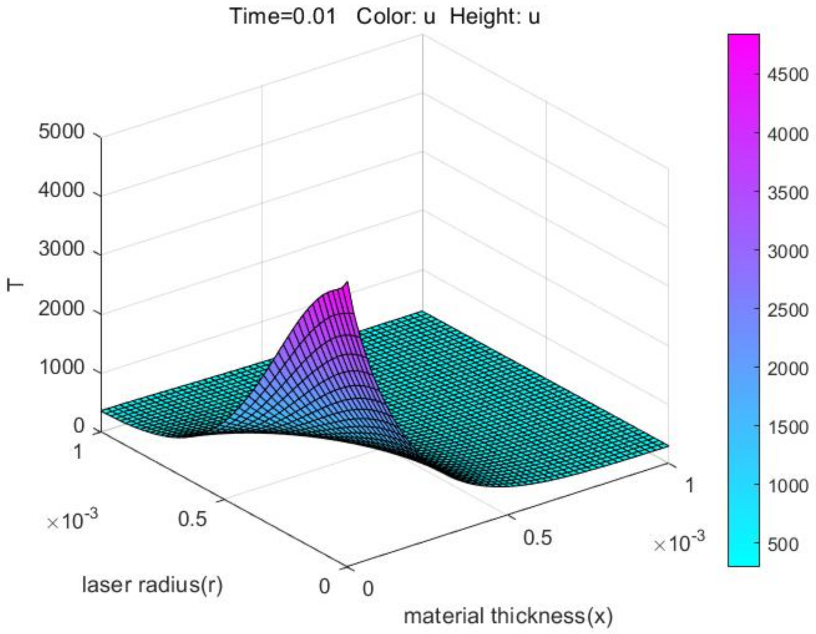
Using ADI with the backward Euler method and ADI with Crank–Nicolson method to solve the problem on MATLAB, we can obtain
Figure 10 and
Figure 11.
Figure 10 shows the numerical solutions of difference equations by ADI with the backward Euler method when
,
and
.
Figure 11 shows the numerical solutions of difference equations by ADI with Crank-Nicolson method when
,
and
.
The laser source is a function of , and the temperature is symmetrically distributed along the radius of the material. Therefore, the temperature becomes lower in the direction, distributed along the laser source function in the direction.
Table 6 is the maximum error and the maximum relative error between the numerical solutions of the ADI with the backward Euler method and the exact solutions of ADI with Crank–Nicolson method when the asynchronous step length is taken.
The maximum relative error is the maximum error divided by the corresponding exact solution.
From
Table 6, when
gets smaller, the maximum error and the maximum relative error of the two algorithms gets smaller. The smaller
, the less the maximum error and the maximum relative error of the two algorithms when
comes the same.
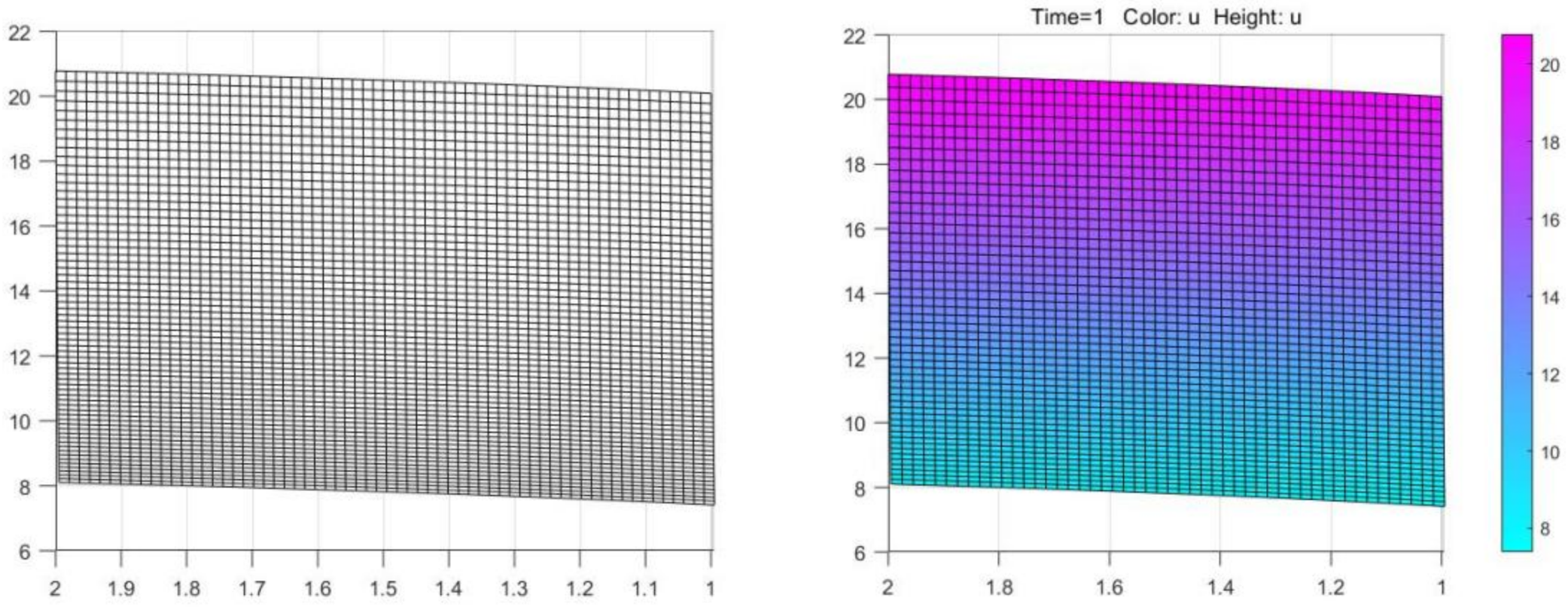
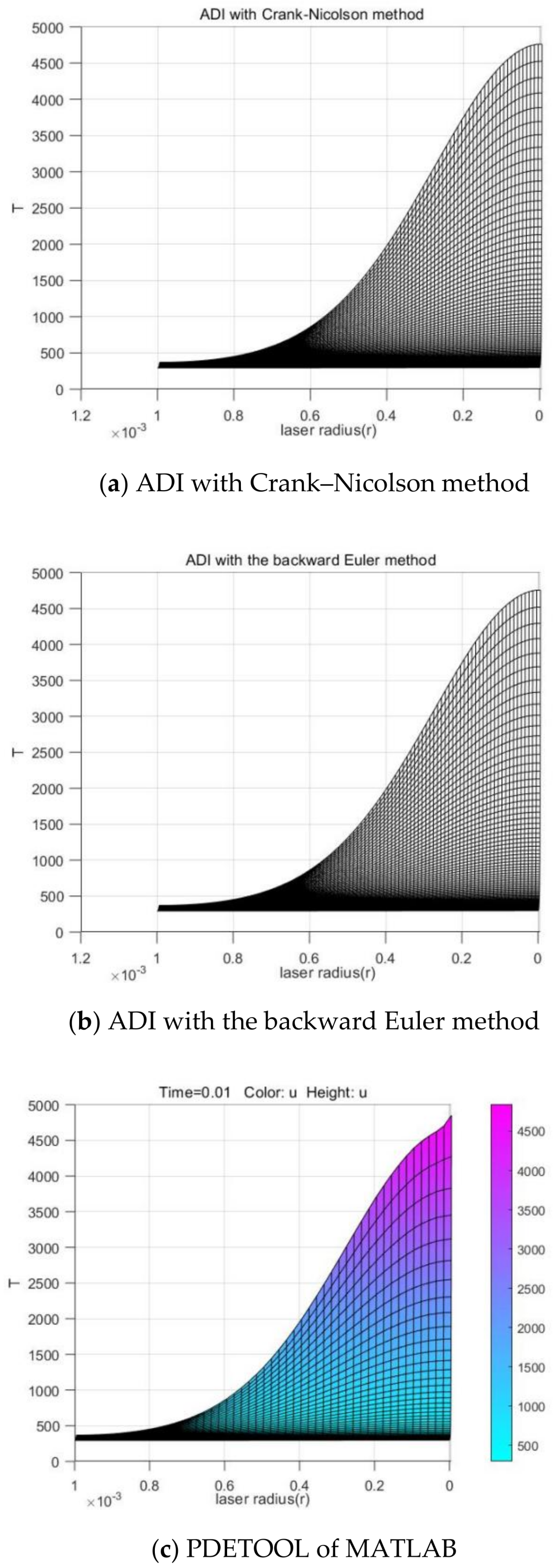
Use the PDETOOL of MATLAB to simulate Example 3. The results are shown in
Figure 12.
From
Figure 10,
Figure 11,
Figure 12,
Figure 13 and
Figure 14, both numerical solutions obtained by the ADI with the backward Euler method and with Crank–Nicolson method for the third kind of boundary value are in good agreement with the numerical solutions given by the PDETOOL of MATLAB in the same environment within a certain small error, which shows that these methods are feasible and effective in laser processing.
Example 4. To be compared with Example 3, we take the laser radius asso that the laser radius is smaller than the material radius under the same environmental conditions.
- (1)
In the laser irradiation surface, we have:
- (2)
The input of laser energy acts on the material surface in the form of Gaussian heat flux, specifically:
Other parameters and environmental conditions behavior the same as Example 3.
Using the ADI with Crank–Nicolson method to solve the problem on MATLAB, we can obtain
Figure 15.
Figure 15 shows the numerical solutions of difference equations by ADI with Crank-Nicolson method when
,
and
.
Use the PDETOOL of MATLAB to simulate Example 4. The results are shown in
Figure 16.
We consider combining the
of Example 4 and the rest of the environmental conditions of Example 3 to form a new problem. This new problem and Example 4 vary from the laser irradiation area. Using ADI with Crank–Nicolson method to solve this new problem on MATLAB, we can attain
Figure 17.
Figure 17 shows the numerical solutions of difference equations by ADI with Crank-Nicolson method when
,
and
.
From
Figure 15 and
Figure 17, the maximum error and the maximum relative error obviously appear on the boundary. Since the maximum error and the maximum relative error respectively is 8.5667 K and 0.0284, and the melting point of the material is relatively high, the temperature distinction in the interior point is negligible in
Figure 15 and
Figure 17.
6. Conclusions
In this article, the effective computation of the heat distribution of the material is studied when the laser beam is irradiated on the section of the cylinder material, where the laser beam is expressed as a Gaussian distribution. The mathematical model—three-dimensional heat conduction equation, is converted into a two-dimensional parabolic equation. Based on the symmetry of the heat distribution, the three-dimensional equation in the rectangular coordinate system can be changed to the simplified two-dimensional equation in the cylindrical coordinate system, which raises the work efficiency, but also saves the storage space.
Subsequently, to solve the simplified equation, the unconditionally stable ADI scheme is developed with the classic backward Euler method or Crank–Nicolson method in the cylindrical coordinate system, and then the simulation results are obtained, where the first kind of boundary value condition or the third kind of boundary value condition is considered. Further, these two methods have been proved to be unconditionally stable and convergent, and their accuracies are verified by Examples 1 and 2. Examples 3 and 4 demonstrate that these two methods are feasible, stable, and efficient to solve the laser processing problem model. Example 4 also verifies that under certain conditions and errors, the entire laser irradiation can be used to replace the partial laser irradiation, thereby simplifying the boundary heat dissipation problem.
Comparison between the results obtained by these two methods and the results obtained by PDETOOL of MATLAB in each example, shows that our results are more convincing, and our treatment has two advantages. Firstly, self-programming can use different methods to discretize distinct problems, which improves the flexibility of the algorithm, saves running space and time and raises efficiency. Secondly, in the absence of an exact solution, our approach can check whether the algorithm is correct or not by comparing with the numerical solution of PDETOOL.
The three-dimensional heat conduction problem model of the article is also universal. The material irradiated by the laser is not necessarily cylindrical. As long as a circle is set at the center of the laser spot, the problem model in this article is still applicable. The only difference is the processing of the boundary, that is, the expression and discretization of the boundary conditions may need to be processed separately.


