A New Hybrid Three-Term Conjugate Gradient Algorithm for Large-Scale Unconstrained Problems

Abstract

Three-term conjugate gradient methods have attracted much attention for large-scale unconstrained problems in recent years, since they have attractive practical factors such as simple computation, low memory requirement, better descent property and strong global convergence property. In this paper, a hybrid three-term conjugate gradient algorithm is proposed and it owns a sufficient descent property, independent of any line search technique. Under some mild conditions, the proposed method is globally convergent for uniformly convex objective functions. Meanwhile, by using the modified secant equation, the proposed method is also global convergence without convexity assumption on the objective function. Numerical results also indicate that the proposed algorithm is more efficient and reliable than the other methods for the testing problems.

1. Introduction

In this paper, we consider the following unconstrained problem:

$$\underset{x\in R^n}{min}f\left(x\right),$$

(1)

where function $f:R^n\to R$ is continuously differentiable and bounded below. There are many methods for solving (1). such as the Levenberg–Marquardt methods [1], Newton methods [2] and quasi-Newton methods [3,4]. However, these methods are efficient for small and medium-sized problems and are not suitable for large scale problems in terms of the storage of a matrix for second order information or its approximation. Conjugate gradient (CG) methods [4,5,6,7,8,9,10,11,12] are much more effective for unconstrained problems, especially for large-scale cases by low memory requirements and strong convergence properties [6,8,9,10,11], etc. Meanwhile, CG methods have been applied to image restoration problems, optimal control problems and optimal problems in machine learning [13,14,15], etc. In this paper, we design a CG method for (1).

The nonlinear CG method was first proposed by Hestenes and Stiefel [16] for linear equations $Ax=b$. In 1964, Fletcher and Reeves [17] extended the CG method in [16] to unconstrained optimization problems. After that, many researchers proposed various CG methods [6,7,8,9,10,12,18]. In CG methods, a sequence of iterative point $\left\{x_k\right\}$ is generated by an initial point $x_0$ and:

$$x_{k+1}=x_k+{\alpha }_k{d}_k,\forall k\ge 0,$$

(2)

where ${\alpha }_k$ is the step size which is determined by some line search technique and $d_k$ is the search direction. In a traditional CG method, the direction is usually defined by

$$\begin{array}{c}\hfill d_k=\left\{\begin{array}{cc}-g_k,\hfill & \mathrm{if}k=0,\hfill \\ -g_k+{\beta }_k{d}_{k-1},\hfill & \mathrm{if}k\ge 1.\hfill \end{array}\right.\end{array}$$

(3)

Different conjugate parameter ${\beta }_k$ generates a different CG method which may be significantly different in theoretical properties and numerical performance. The Hestenes–Stiefel (HS) method [16] and Polak–Ribière–Polyak (PRP) method [19,20] have nice numerical performance and their conjugate parameters are:

$${\beta }_{k+1}^{HS}=\frac{g_{k+1}^T{y}_k}{d_k^T{y}_k},{\beta }_{k+1}^{PRP}=\frac{g_{k+1}^T{y}_k}{\parallel g_k{\parallel }^2},$$

where $g_k=\nabla f\left(x_k\right)$, $g_{k+1}=\nabla f\left(x_{k+1}\right)$ and $y_k=g_{k+1}-g_k$. Note that the HS method automatically satisfies the conjugate condition $d_{k+1}^T{y}_k=0$, independently of any line search technique. Dai and Liao [18] extended the above conjugate condition to:

$$d_{k+1}^T{y}_k=-t{g}_{k+1}^T{s}_k,\forall k\ge 1.$$

(4)

where $t\ge 0$ and $s_k=x_{k+1}-x_k$. The new condition (4) gives a more accurate approximation for the Hessian matrix of the original objective function. Based on the condition (4), Dai and Liao [18] presented a new conjugate parameter:

$${\beta }_{k+1}^{DL}\left(t\right)=\frac{g_{k+1}^T(y_k-t{s}_k)}{y_k^T{d}_k}=\frac{g_{k+1}^T{y}_k}{y_k^T{d}_k}-t\frac{g_{k+1}^T{s}_k}{y_k^T{d}_k}.$$

(5)

In order to have global convergence, they selected the non-negative conjugate parameter, meaning that:

$${\beta }_{k+1}^{DL+}\left(t\right)=max\{0,{\beta }_{k+1}^{DL}\left(t\right)\}.$$

Under some mild conditions, the global convergence was established. However, the selection of the parameter t strongly affects the numerical performance, thus many scholars have focused on the choices for the parameter t, as can be seen in [21,22,23,24,25,26] etc.

Compared with the traditional two-term CG method, three-term CG methods [27,28,29,30,31] always have good numerical performance and nice theoretical properties, such as the sufficient descent property, independently of the accuracy of line search, i.e., it is always holds that:

$$g_k^T{d}_k\le -c{\parallel g_k\parallel }^2,$$

where $c>0$. Specifically, Zhang et al. [29] proposed a descent three-term PRP CG method in which the direction has the form:

$$d_0=-g_0,d_{k+1}=-g_{k+1}+{\beta }_{k+1}^{PRP}{d}_k+{\delta }_{k+1}^{PRP}{y}_k,{\delta }_{k+1}^{PRP}=-\frac{g_{k+1}^T{d}_k}{\parallel g_k{\parallel }^2},k\ge 0.$$

(6)

and Zhang et al. [28] presented a descent three-term HS CG method in which the direction is:

$$d_0=-g_0,d_{k+1}=-g_{k+1}+{\beta }_{k+1}^{HS}{d}_k+{\delta }_{k+1}^{HS}{y}_k,{\delta }_{k+1}^{HS}=-\frac{g_{k+1}^T{d}_k}{d_k^T{y}_k},k\ge 0.$$

(7)

and Babaie-Kafaki and Ghanbari [31] gave a modified three-term HS/DL method in which the direction owns the form:

$$d_0=-g_0,d_{k+1}=-g_{k+1}+{\beta }_{k+1}^{HS}{d}_k-t\frac{g_{k+1}^T{s}_k}{|y_k^T{d}_k|}{d}_k+{\delta }_{k+1}^{HS}{y}_k,{\delta }_{k+1}^{HS}=-\frac{g_{k+1}^T{d}_k}{d_k^T{y}_k},k\ge 0.$$

(8)

For the above three directions, the sufficient descent property is always satisfied, i.e., $g_k^T{d}_k\le -{\parallel g_k\parallel }^2$. Note that the sufficient descent property is stronger that the descent property and may greatly improve the numerical performance of the corresponding methods.

Motivated by the above discussions, in this paper, we propose a new descent hybrid three-term CG algorithm. Under some mild conditions, the direction in this descent hybrid three-term CG algorithm may reduce the directions in [28,29,31], respectively, and another new three-term direction which also satisfies the sufficient descent property with $c=1$ (which is why we call our method as the hybrid three-term CG method). The new method owns the sufficient descent property independent of the accuracy of the line search technique. Under some mild conditions, the global convergence is established for uniformly convex objective functions. For general functions without convexity assumption, the global convergence is also established by using the modified secant condition in [32]. Numerical results indicate that the proposed algorithm is effective and reliable.

The paper is organized as follows. In Section 2, we firstly present the motivation for the hybrid three-term CG method and then propose the new hybrid three-term direction and prove some properties of the new direction and give the global convergence for uniformly convex objective functions at last. In Section 3, the global convergence for the general nonlinear functions is established with the help of the modified secant condition. Numerical tests are given in Section 4 to show the efficient and reliable nature of the proposed algorithm. Finally, the conclusions are presented in Section 5.

2. Motivation and Algorithm

In this section, we firstly present the motivation and give the form of the new direction.

It should be noted that if the exact line search technique is adopted, which implies $g_{k+1}^T{d}_k=0$, then it holds that:

$${\beta }_{k+1}^{HS}={\beta }_{k+1}^{PRP}={\beta }_{k+1}^{DL}\left(t\right).$$

If the inexact line search technique is adopted, these three methods may be different in theoretical property and numerical performance and the HS method and DL method may be not well defined (the denominator $y_k^T{d}_k$ may be 0). Zhang [33] present a hybrid conjugate parameter ${\beta }_{k+1}^{hybrid}$ for the traditional two-term Dai–Liao CG method:

$${\beta }_{k+1}^{hybrid}=\frac{g_{k+1}^T(y_k-t{s}_k)}{max\{y_k^T{d}_k,\parallel g_k{\parallel }^2\}}.$$

The numerical results for general nonlinear equations show that the hybrid two-term conjugate residual method is effective and reliable.

Motivated by the above discussions and the nice properties of three-term CG methods, in the following, we propose a new hybrid descent three-term direction which has the following form: $d_0=-g_0$ and:

$$d_{k+1}^N=-g_{k+1}+{\beta }_{k+1}^N{\mathbf{s}}_{\mathbf{k}}-{\delta }_{k+1}^N{y}_k,$$

(9)

where:

$${\beta }_{k+1}^N=\frac{g_{k+1}^T(y_k-t{s}_k)}{max\{{\mathbf{y}}_{\mathbf{k}}^{\mathbf{T}}{\mathbf{s}}_{\mathbf{k}},\parallel g_k{\parallel }^2\}},{\delta }_{k+1}^N=\frac{g_{k+1}^T{s}_k}{max\{{\mathbf{y}}_{\mathbf{k}}^{\mathbf{T}}{\mathbf{s}}_{\mathbf{k}},\parallel g_k{\parallel }^2\}}.$$

Note that the direction $d_{k+1}^N$ is well defined. In fact, if $y_k^T{s}_k={\parallel g_k\parallel }^2=0$ holds, the condition $\parallel g_k{\parallel }^2=0$ indicates that the method stops and the optimal solution ($x_k$) is obtained.

In the following, we give some remarks for the above direction. Note that if $t=0$ and $y_k^T{s}_k\ge {\parallel g_k\parallel }^2$ hold, the direction $d_{k+1}^N$ reduces the direction $d_{k+1}^{TTHS}$ in [28], and $t=0$ and $y_k^T{s}_k\le {\parallel g_k\parallel }^2$ hold, the direction $d_{k+1}^N$ reduces to the direction $d_{k+1}^{TTPRP}$ in [29]. Note also that if $y_k^T{s}_k\ge {\parallel g_k\parallel }^2$ holds, then the parameter ${\beta }_{k+1}^N$ reduces to the conjugate parameter ${\beta }_{k+1}^{DL}$ and the direction $d_{k+1}^N$ reduces to a modified vision of the direction $d_{k+1}^{TTDL}$ in [31]. If $y_k^T{s}_k<{\parallel g_k\parallel }^2$ holds, the direction $d_{k+1}^N$ reduces to a new three-term direction which also satisfies the sufficient descent property with $c=1$. Overall, we regard the direction $d_{k+1}^N$ as the hybrid direction of the HS direction, the Dai–Liao direction and the PRP direction.

2.1. Algorithm for Uniformly Convex Functions

Now, based on the above analyses, we state the steps of our algorithm as follows:

Algorithm 1: New hybrid three-term conjugate gradient method (HTTCG).

1  Step 0. Select the initial point $x_0\in {\mathbb{R}}^n$. Compute $g\left(x_0\right)$ and set $d_0=-g_0$. Let $k:=0$. 2  Step 1. If $\parallel g_k\parallel \le \epsilon$, then stop, otherwise go to next step; 3  Step 2. Compute the step size ${\alpha }_k$ along the direction $d_k$ by the line search strategy technique; 4  Step 3. Let $x_{k+1}=x_k+{\alpha }_k{d}_k$; 5  Step 4. Compute the search direction $d_{k+1}$ by (9); 6  Step 5. Set $k:=k+1$ and go to Step 1.

Remark 1.

Note that in Algorithm 1, the line search technique is not explicitly given. In fact, any line search technique is accepted.

In the following, we show that Algorithm 1 owns the sufficient descent property independent of any line search technique.

Lemma 1.

For any line search technique, the sequence $\left\{d_k^N\right\}$ is generated by Algorithm 1, and it always holds that:

$$g_k^T{d}_k^N\le -{\parallel g_k\parallel }^2,\forall k\ge 0.$$

(10)

Proof. 

If $k=0$, we have $d_0=-g_0$, then it holds $g_0^T{d}_0=-{\parallel g_0\parallel }^2$. For $k\ge 0$, by the definition of $d_{k+1}^N$, we have the following inequality:

$$\begin{array}{ccc}{g}_{k+1}^T{d}_{k+1}^N\hfill & =\hfill & -\parallel g_{k+1}{\parallel }^2+\frac{g_{k+1}^T(y_k-t{s}_k)}{max\{y_k^T{s}_k,\parallel g_k{\parallel }^2\}}{g}_{k+1}^T{s}_k-\frac{g_{k+1}^T{s}_k}{max\{y_k^T{s}_k,\parallel g_k{\parallel }^2\}}{g}_{k+1}^T{y}_k\hfill \\ \hfill & =\hfill & -\parallel g_{k+1}{\parallel }^2+\frac{g_{k+1}^T{s}_k{g}_{k+1}^T{y}_k}{max\{y_k^T{s}_k,\parallel g_k{\parallel }^2\}}-\frac{t{\left(g_{k+1}^T{s}_k\right)}^2}{max\{y_k^T{s}_k,\parallel g_k{\parallel }^2\}}-\frac{g_{k+1}^T{s}_k{g}_{k+1}^T{y}_k}{max\{y_k^T{s}_k,\parallel g_k{\parallel }^2\}}\hfill \\ \hfill & =\hfill & -\parallel g_{k+1}{\parallel }^2-\frac{t{\left(g_{k+1}^T{s}_k\right)}^2}{max\{y_k^T{s}_k,\parallel g_k{\parallel }^2\}}\hfill \\ \hfill & \le \hfill & -\parallel g_{k+1}{\parallel }^2,\hfill \end{array}$$

(11)

where the last inequality holds by $t\ge 0$. Then, (10) holds. This completes the proof. □

Lemma 1 means that the new direction satisfies the sufficient descent property independent of the line search technique. A conjugate condition also plays an important role in numerical performance. In the HS method, it automatically satisfies the condition $d_{k+1}^T{y}_k=0$; in Dai–Liao method, the modified condition $d_{k+1}^T{y}_k=-t{g}_{k+1}^T{s}_k$ is always satisfied. In our part, by the design of the direction $d_{k+1}^N$, we have:

$$\begin{array}{ccc}{\left(d_{k+1}^N\right)}^T{y}_k\hfill & =\hfill & -g_{k+1}^T{y}_k+\frac{g_{k+1}^T(y_k-t{s}_k)}{max\{y_k^T{s}_k,\parallel g_k{\parallel }^2\}}{y}_k^T{s}_k-\frac{g_{k+1}^T{s}_k}{max\{y_k^T{s}_k,\parallel g_k{\parallel }^2\}}{\parallel y_k\parallel }^2\hfill \\ \hfill & =\hfill & -g_{k+1}^T{y}_k+\frac{y_k^T{s}_k}{max\{y_k^T{s}_k,\parallel g_k{\parallel }^2\}}{g}_{k+1}^T{y}_k-\frac{y_k^T{s}_k\left(t{g}_{k+1}^T{s}_k\right)}{max\{y_k^T{s}_k,\parallel g_k{\parallel }^2\}}-\frac{\parallel y_k{\parallel }^2\left(g_{k+1}^T{s}_k\right)}{max\{y_k^T{s}_k,\parallel g_k{\parallel }^2\}}\hfill \\ \hfill & \le \hfill & -\frac{t{y}_k^T{s}_k+{\parallel y_k\parallel }^2}{max\{y_k^T{s}_k,\parallel g_k{\parallel }^2\}}{g}_{k+1}^T{s}_k.\hfill \end{array}$$

(12)

From (12), it holds that the new direction $d_{k+1}^N$ also satisfies the DL conjugate condition (4) in an extent form, i.e., ${\left(d_{k+1}^N\right)}^T{y}_k\le -t_1{g}_{k+1}^T{s}_k$ where $t_1=\frac{t{y}_k^T{s}_k+{\parallel y_k\parallel }^2}{max\{y_k^T{s}_k,\parallel g_k{\parallel }^2\}}$. In fact, if we adopt the line search technique which results in $y_k^T{s}_k\ge 0$, then it holds that $t_1=\frac{t{y}_k^T{s}_k+{\parallel y_k\parallel }^2}{max\{y_k^T{s}_k,\parallel g_k{\parallel }^2\}}>0$.

2.2. Convergence for Uniformly Convex Functions

In the following, we present the global convergence analysis of the HTTCG method under the following assumptions.

Assumption 1.

The level set $\mathbb{T}:=\{x\in {\mathbb{R}}^n:f\left(x\right)\le f\left(x_0\right)\}$ is bounded where $x_0$ is the starting point, namely, there exists a constant $X>0$ such that:

$$\parallel x\parallel \le X,\forall x\in \mathbb{T}.$$

(13)

Assumption 2.

In some neighborhood $\mathbb{N}$ of $\mathbb{T}$, the gradient of function $f\left(x\right)$, $g\left(x\right)$, is Lipschitz continuous, which means there exists a constant $L>0$ such that:

$$\parallel g\left(x\right)-g\left(y\right)\parallel \le L\parallel x-y\parallel ,\forall x,y\in \mathbb{N}.$$

(14)

Note that based on Assumptions 1 and 2, there exists a positive constant G such that:

$$\parallel g\left(x\right)\parallel \le G,\forall x\in \mathbb{T}.$$

(15)

In the following, we show that the sequence $\left\{d_k^N\right\}$ generated by Algorithm 1 is bounded.

Lemma 2.

Assume $0<t\le T$ and Assumptions 1 and 2 hold. For any line search technique, the sequence $\left\{d_k^N\right\}$ is generated by Algorithm 1. If the objective function f is uniformly convex on the set $\mathbb{N}$, then $\left\{d_k^N\right\}$ is bounded.

Proof. 

Since function f is uniformly convex on the set $\mathbb{N}$, then for any $x,y\in \mathbb{N}$, we have

$${(\nabla f\left(x\right)-\nabla f\left(y\right))}^T(x-y)\ge \mu {\parallel x-y\parallel }^2,$$

where $\mu >0$ is the uniformly convex parameter. Especially, if we take $x=x_{k+1}$ and $y=x_k$, then it holds that:

$$y_k^T{s}_k\ge \mu {\parallel s_k\parallel }^2>0.$$

(16)

In the following, we prove the boundedness of parameters ${\beta }_{k+1}^N$ and ${\delta }_{k+1}^N$. In fact, by their definitions, we have:

$$\begin{array}{ccc}|{\beta }_{k+1}^N|\hfill & =\hfill & \left|\frac{g_{k+1}^T(y_k-t{s}_k)}{max\{y_k^T{s}_k,\parallel g_k{\parallel }^2\}}\right|\le \frac{\parallel g_{k+1}\parallel (\parallel y_k\parallel +t\parallel s_k\parallel )}{|max\{y_k^T{s}_k,\parallel g_k{\parallel }^2\left\}\right|}\le \frac{\parallel g_{k+1}\parallel (\parallel y_k\parallel +t\parallel s_k\parallel )}{y_k^T{s}_k}\hfill \\ \hfill & \le \hfill & \frac{(L+T)\parallel s_k\parallel }{\mu \parallel s_k{\parallel }^2}\parallel g_{k+1}\parallel =\frac{L+T}{\mu }\frac{\parallel g_{k+1}\parallel }{\parallel s_k\parallel },\hfill \end{array}$$

(17)

$$\begin{array}{ccc}|{\delta }_{k+1}^N|\hfill & =\hfill & \left|\frac{g_{k+1}^T{s}_k}{max\{y_k^T{s}_k,\parallel g_k{\parallel }^2\}}\right|\le \frac{\parallel g_{k+1}\parallel \parallel s_k\parallel }{|max\{y_k^T{s}_k,\parallel g_k{\parallel }^2\left\}\right|}\le \frac{\parallel g_{k+1}\parallel \parallel s_k\parallel }{y_k^T{s}_k}\hfill \\ \hfill & \le \hfill & \frac{\parallel g_{k+1}\parallel \parallel s_k\parallel }{\mu \parallel s_k{\parallel }^2}=\frac{1}{\mu }\frac{\parallel g_{k+1}\parallel }{\parallel s_k\parallel },\hfill \end{array}$$

(18)

By the definition of $d_{k+1}^N$, we have:

$$\begin{array}{ccc}\parallel d_{k+1}^N\parallel \hfill & \le \hfill & \parallel g_{k+1}\parallel +|{\beta }_{k+1}^N|\parallel s_k\parallel +|{\delta }_{k+1}^N|\parallel y_k\parallel \hfill \\ \hfill & \le \hfill & \parallel g_{k+1}\parallel +\frac{L+T}{\mu }\frac{\parallel g_{k+1}\parallel }{\parallel s_k\parallel }\parallel s_k\parallel +\frac{1}{\mu }\frac{\parallel g_{k+1}\parallel }{\parallel s_k\parallel }\parallel y_k\parallel \hfill \\ \hfill & \le \hfill & \parallel g_{k+1}\parallel +\frac{L+T}{\mu }\parallel g_{k+1}\parallel +\frac{L}{\mu }\parallel g_{k+1}\parallel \hfill \\ \hfill & =\hfill & \left(1+\frac{2L+T}{\mu }\right)\parallel g_{k+1}\parallel \le \left(1+\frac{2L+T}{\mu }\right)G,\hfill \end{array}$$

(19)

where the last inequality holds by (15). This completes the proof. □

The standard Wolfe line search technique is often referred to in CG methods (see [6,7,11] etc.). It has the following form:

$$\left\{\begin{array}{c}f(x_k+{\alpha }_k{d}_k)\le f\left(x_k\right)+{\sigma }_1{\alpha }_k{g}_k^T{d}_k,\hfill \\ g{(x_k+{\alpha }_k{d}_k)}^T{d}_k\ge {\sigma }_2{g}_k^T{d}_k,\hfill \end{array}\right.$$

(20)

where $0<{\sigma }_1<{\sigma }_2<1$.

The following lemma plays an essential role for the global convergence theorem of our method. It can be seen in Lemma 3.1 in [34]. Hence, we only state it here and omit its proof.

Lemma 3.

Suppose that Assumptions 1 and 2 hold. Consider any iterative method with the form (2) where $d_k$ satisfies the sufficient descent property and ${\alpha }_k$ is computed by Wolfe line search technique (20). If the following relationship holds:

$$\sum _{k\ge 0}\frac{1}{\parallel d_k{\parallel }^2}=+\infty ,$$

(21)

then the method globally converges in the sense that:

$$\underset{k\to +\infty }{lim\; inf}\parallel g_k\parallel =0.$$

(22)

Now, we establish the global convergence of Algorithm 1 for the uniformly convex objective functions.

Theorem 1.

Suppose that Assumptions 1 and 2 hold. Consider Algorithm 1 in which step size ${\alpha }_k$ is computed by the line search technique (20). If the objective function f is uniformly convex on set $\mathbb{N}$, then Algorithm 1 globally converges in the sense that:

$$\underset{k\to +\infty }{lim}\parallel g_k\parallel =0.$$

(23)

Proof. 

From Lemma 1, we have that the direction $d_{k+1}^N$ satisfies the sufficient descent property with $c=1$. By the first inequality in the line search technique (20), we have the sequence ${\left\{f\left(x_k\right)\right\}}_{k\ge 0}$ is non-increasing and ${\left\{x_k\right\}}_{k\ge 0}\subseteq \mathbb{N}$. By the boundedness of $\left\{d_k^N\right\}$ in Lemma 2, we have that (21) holds. Then, (22) holds. Since f is uniformly convex, then we have (23). This completes the proof. □

3. Convergence for General Nonlinear Functions

In order to achieve the global convergence without convexity assumption for the general function, we adopt the modified secant condition in [32] (similar modified secant conditions can also be founded in [35,36] etc.). Concretely, the modified secant condition is:

$${\nabla }^{2}f\left(x_{k+1}\right)s_k=z_k,$$

where $p>0$ and $C>0$ and:

$$z_k=y_k+h_k\parallel g_k{\parallel }^p{s}_k,h_k=C+max\left\{0,-\frac{y_k^T{s}_k}{\parallel s_k{\parallel }^2}\right\}{\parallel g_k\parallel }^{-p}.$$

(24)

Based on the modified secant condition, we present the direction: $d_0=-g_0$ and:

$$d_{k+1}^{NN}=-g_{k+1}+{\beta }_{k+1}^{NN}{s}_k-{\delta }_{k+1}^{NN}{z}_k,$$

(25)

where:

$${\beta }_{k+1}^{NN}=\frac{g_{k+1}^T(z_k-t{s}_k)}{max\{z_k^T{s}_k,\parallel g_k{\parallel }^2\}},{\delta }_{k+1}^{NN}=\frac{g_{k+1}^T{s}_k}{max\{z_k^T{s}_k,\parallel g_k{\parallel }^2\}}.$$

Now, based on the above discussions, we state our algorithm as follows:

Algorithm 2: Hybrid three-term CG method using modified secant condition (HTTCGSC).

1  Step 0. Select $x_0\in {\mathbb{R}}^n$, constants $C>0$ and $r>0$. Compute $g\left(x_0\right)$ and set $d_0=-g_0$. Let $k:=0$. 2  Step 1. If $\parallel g_k\parallel \le \epsilon$, then stop, otherwise go to next step; 3  Step 2. Compute the step size ${\alpha }_k$ along the direction $d_k$ by the line search technique; 4  Step 3. Let $x_{k+1}=x_k+{\alpha }_k{d}_k$; 5  Step 4. Compute the search direction $d_{k+1}$ by (25); 6  Step 5. Set $k:=k+1$ and go to Step 1.

Note also that in Algorithm 2, the line search technique is not explicitly given. Similar to Lemma 1, we also have the following lemma. Here, we omit its proof.

Lemma 4.

For any line search technique, the sequence $\left\{d_k^{NN}\right\}$ is generated by Algorithm 2, then it always holds that:

$$g_k^T{d}_k^{NN}\le -{\parallel g_k\parallel }^2,\forall k\ge 0.$$

(26)

Lemma 5.

The sequences $\left\{z_k\right\}$ and $\left\{s_k\right\}$ are generated by Algorithm 2, then for any line search technique, we have:

$$z_k^T{s}_k\ge C{\parallel g_k\parallel }^p{\parallel s_k\parallel }^2,$$

(27)

and:

$$\parallel z_k\parallel \le (2L+C{G}^p)\parallel s_k\parallel .$$

(28)

Proof. 

In fact, for any line search technique, we consider two cases:

Case (i) $y_k^T{s}_k\ge 0$ holds. In this case, we have $h_k=C$ and $z_k=y_k+C{\parallel g_k\parallel }^p{s}_k$. Then, we have:

$$z_k^T{s}_k=y_k^T{s}_k+C{\parallel g_k\parallel }^p{\parallel s_k\parallel }^2\ge C{\parallel g_k\parallel }^p{\parallel s_k\parallel }^2.$$

(29)

Case (ii) $y_k^T{s}_k<0$ holds. In this case, it holds that $h_k=C-\frac{y_k^T{s}_k}{\parallel s_k{\parallel }^2}{\parallel g_k\parallel }^{-p}$ and $z_k=y_k+C{\parallel g_k\parallel }^p{s}_k-\frac{y_k^T{s}_k}{\parallel s_k{\parallel }^2}{s}_k$. Then, we have:

$$z_k^T{s}_k=y_k^T{s}_k+C{\parallel g_k\parallel }^p{\parallel s_k\parallel }^2-y_k^T{s}_k\ge C{\parallel g_k\parallel }^p{\parallel s_k\parallel }^2.$$

(30)

Based on the above discussions, we have that for any line search technique, (27) always holds.

By the definition of $z_k$, we have:

$$\parallel z_k\parallel \le \parallel y_k\parallel +|h_k|{\parallel g_k\parallel }^p\parallel s_k\parallel \le L\parallel s_k\parallel +\left(C+\frac{|y_k^T{s}_k|}{\parallel s_k{\parallel }^2}{\parallel g_k\parallel }^{-p}\right){\parallel g_k\parallel }^p\parallel s_k\parallel \le (2L+C{G}^p)\parallel s_k\parallel ,$$

where the last inequality holds by $\parallel g_k\parallel \le G$. Then, (28) holds. This completes the proof. □

In the following, we assume that the limit (22) does not hold, otherwise Algorithm 2 converges. This means that there exists a positive constant $\eta$ such that:

$$\parallel g_k\parallel \ge \eta ,\forall k\ge 0.$$

(31)

Now, we give the global convergence of Algorithm 2 for general nonlinear problems without convex assumption.

Theorem 2.

Suppose that Assumptions 1 and 2 hold. Consider Algorithm 2 in which step size ${\alpha }_k$ is computed by line search technique (20). Then, Algorithm 2 globally converges in the sense that (22) holds.

Proof. 

We proceed by contradiction. Suppose that (22) is not true. Then, the inequality (31) holds.

In the following, we firstly prove that the sequence ${\left\{d_k^{NN}\right\}}_{k\ge 0}$ is bounded. Similarly, due to the analyses in (17) and (18), we have that:

$$\begin{array}{ccc}|{\beta }_{k+1}^{NN}|\hfill & =\hfill & \left|\frac{g_{k+1}^T(z_k-t{s}_k)}{max\{z_k^T{s}_k,\parallel g_k{\parallel }^2\}}\right|\le \frac{\parallel g_{k+1}\parallel (\parallel z_k\parallel +t\parallel s_k\parallel )}{z_k^T{s}_k}\hfill \\ \hfill & \le \hfill & \frac{(2L+C{G}^p+T)\parallel s_k\parallel }{C\parallel g_k{\parallel }^p{\parallel s_k\parallel }^2}\parallel g_{k+1}\parallel \le \frac{2L+C{G}^p+T}{C{\eta }^p}\frac{\parallel g_{k+1}\parallel }{\parallel s_k\parallel },\hfill \end{array}$$

(32)

where the third inequality holds by Assumption 1 and (28), the last inequality holds by $\parallel g_k\parallel \ge \eta$.

$$\begin{array}{ccc}|{\delta }_{k+1}^{NN}|\hfill & =\hfill & \left|\frac{g_{k+1}^T{s}_k}{max\{z_k^T{s}_k,\parallel g_k{\parallel }^2\}}\right|\le \frac{\parallel g_{k+1}\parallel \parallel s_k\parallel }{|max\{z_k^T{s}_k,\parallel g_k{\parallel }^2\left\}\right|}\le \frac{\parallel g_{k+1}\parallel \parallel s_k\parallel }{z_k^T{s}_k}\hfill \\ \hfill & \le \hfill & \frac{\parallel g_{k+1}\parallel \parallel s_k\parallel }{C\parallel g_k{\parallel }^p{\parallel s_k\parallel }^2}\le \frac{1}{C{\eta }^p}\frac{\parallel g_{k+1}\parallel }{\parallel s_k\parallel },\hfill \end{array}$$

(33)

where the last inequality holds by $\parallel g_k\parallel \ge \eta$. Then, by (25), it holds that:

$$\begin{array}{ccc}\parallel d_{k+1}^{NN}\parallel \hfill & \le \hfill & \parallel g_{k+1}\parallel +|{\beta }_{k+1}^{NN}|\parallel s_k\parallel +|{\delta }_{k+1}^{NN}|\parallel z_k\parallel \hfill \\ \hfill & \le \hfill & \parallel g_{k+1}\parallel +\frac{2L+C{G}^p+T}{C{\eta }^p}\frac{\parallel g_{k+1}\parallel }{\parallel s_k\parallel }\parallel s_k\parallel +\frac{1}{C{\eta }^p}\frac{\parallel g_{k+1}\parallel }{\parallel s_k\parallel }\parallel z_k\parallel \hfill \\ \hfill & \le \hfill & \parallel g_{k+1}\parallel +\frac{2L+C{G}^p+T}{C{\eta }^p}\parallel g_{k+1}\parallel +\frac{2L+C{G}^p}{C{\eta }^p}\parallel g_{k+1}\parallel \hfill \\ \hfill & =\hfill & \left(1+\frac{4L+2C{G}^p+T}{C{\eta }^p}\right)\parallel g_{k+1}\parallel \le \left(1+\frac{4L+2C{G}^p+T}{C{\eta }^p}\right)G.\hfill \end{array}$$

(34)

That means the sequence ${\left\{d_k^{NN}\right\}}_{k\ge 0}$ is bounded. Hence, (21) holds. From Lemmas 3 and 4, we have ${lim\; inf}_{k\to +\infty }\parallel g_k\parallel =0$, which contradicts (31). Then, (22) holds. This completes the proof. □

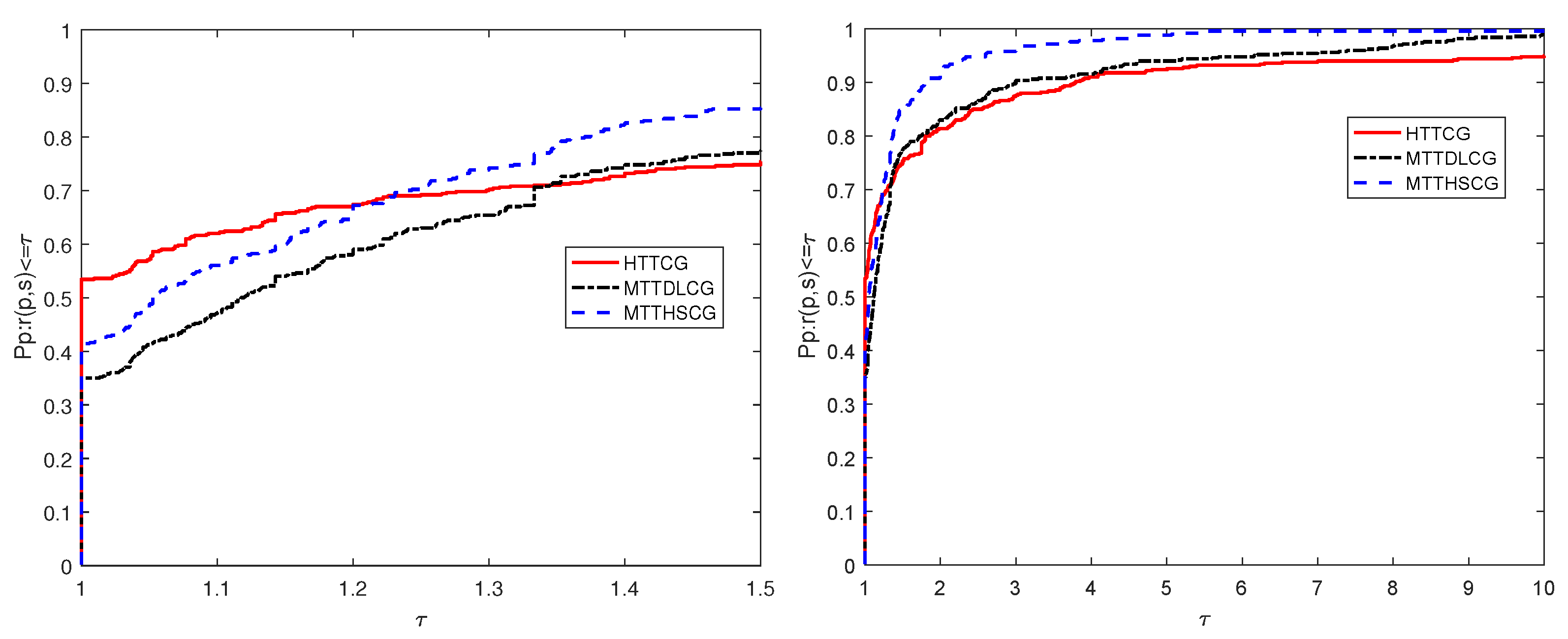
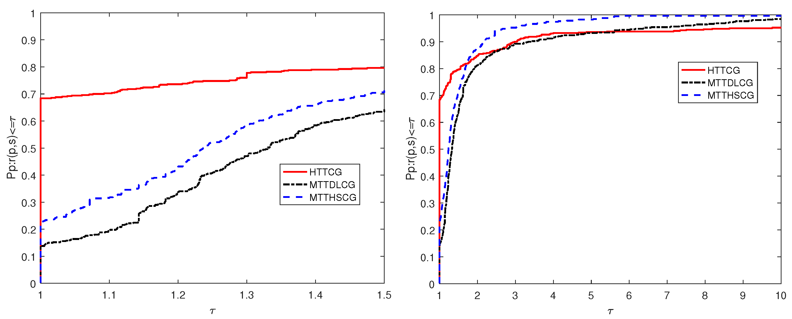
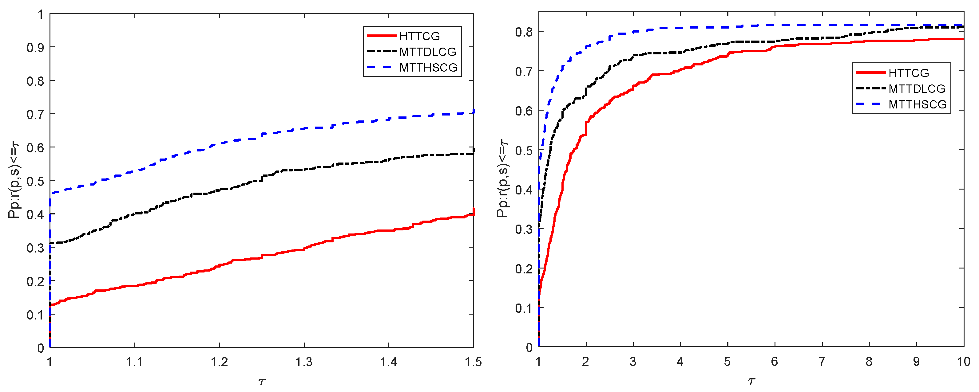
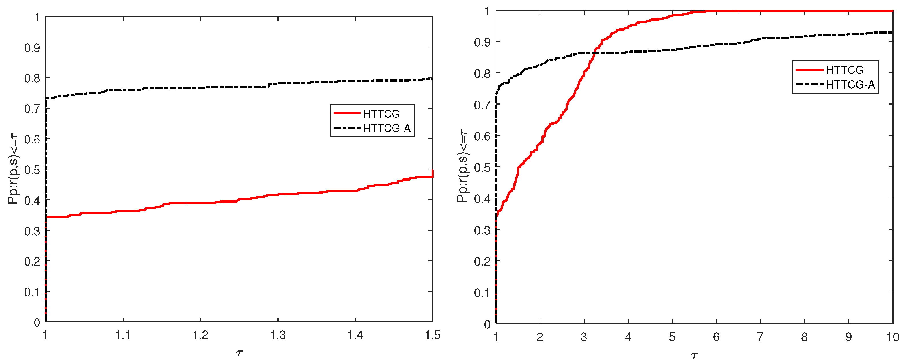
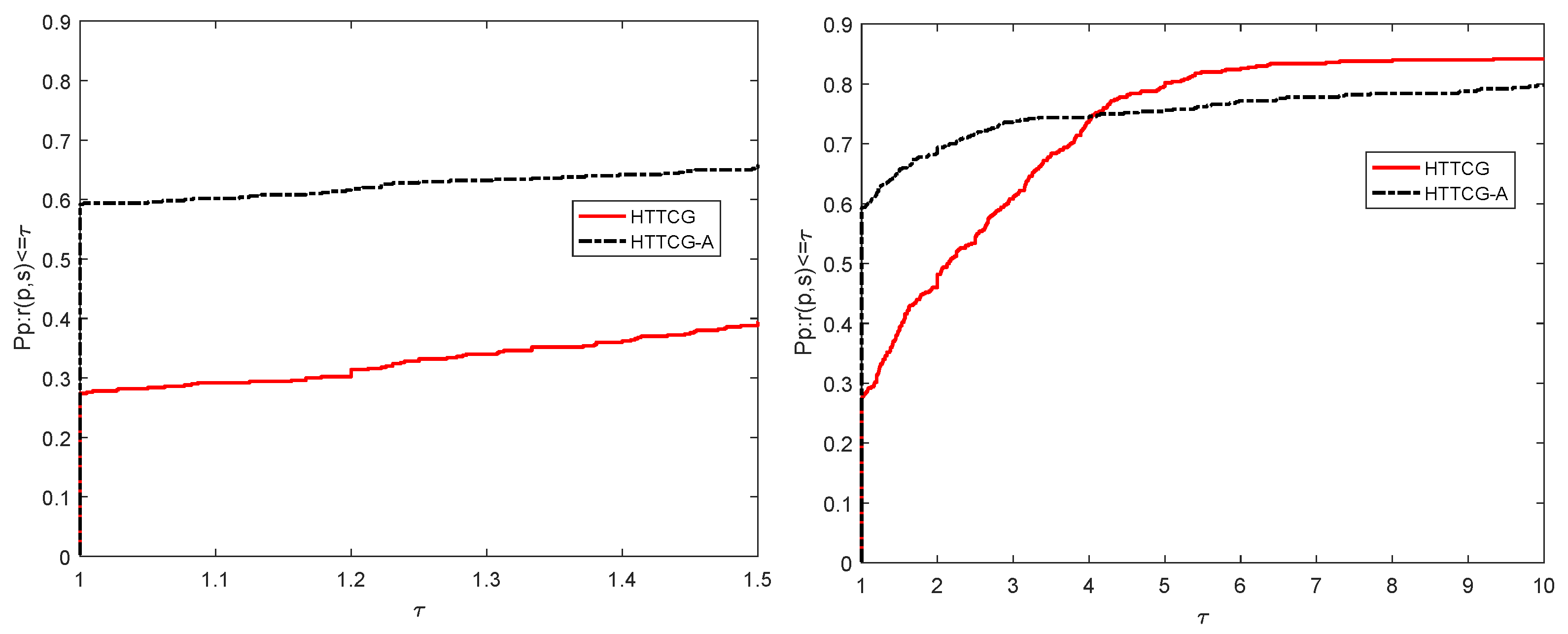
4. Numerical Results

In this section, we firstly present the numerical performance of Algorithm 2 and compare it with other methods in [28,31]. Then, an accelerated technique is applied in our method.

4.1. Numerical Performance of Algorithm 2

In this subsection, we focus on the numerical performance of Algorithm 2 and compare it with the MTTDLCG method in [31] and the MTTHSCG method in [28]. For the MTTDLCG method and the MTTHSCG method, we take their settings for parameters. For the value of parameter t, authors in [37] point out that $t=\frac{\parallel y_k{\parallel }^2}{y_k^T{s}_k}$ is a good choice for the Dai–Liao method and the authors in [18] suggest $t=0.1$ is a good choice. In this paper, we take $t=max\{0.1,\frac{\parallel z_k{\parallel }^2}{max\{z_k^T{s}_k,\parallel g_k{\parallel }^2\}}\}$.

We execute the tests on a personal computer with the Windows 10 operating system, AMD CPU with $@2.1$ GHz, 16.00 GB of RAM. Meanwhile, the corresponding codes are written in MATLAB R2016b. The parameters referred are that: ${\sigma }_1=0.20$, ${\sigma }_2=0.85$, $C=0.1$, $r=1$ if $\parallel s_k{\parallel }^2<1$, $r=3$ otherwise. In the following, we present the stopping rules:

Stopping rules (Himmeblau rule): During the testing, if $|f\left(x_k\right)|>{ϵ}_1$, set $\mathsf{\Delta }=\frac{|f\left(x_k\right)-f\left(x_{k+1}\right)|}{\left|f\right(x_k\left)\right|},$ or let $\mathsf{\Delta }=|f\left(x_k\right)-f\left(x_{k+1}\right)|$. Testing stops if $\parallel g\left(x\right)\parallel <\epsilon$ or Tem $<{\epsilon }_2$ holds. The values of these parameters are ${\epsilon }_1={\epsilon }_2={10}^{-5}$ and $ϵ={10}^{-6}$. Meanwhile, the testing also stops if the total iteration number is larger than 10,000.

For the step size, ${\alpha }_k$ will be chosen when the search number of the WWP line search is more than 6. Testing problems with initial points considered here are from [38], which are listed in

Table 1. The testing problems.

N0	Problem	N0	Problem
1	Extended Trigonometric Function	26	BDQRTIC (CUTE)
2	Extended Rosenbrock Function	27	ARWHEAD (CUTE)
3	Extended White and Holst Function	28	NONDIA (Shanno-78) (CUTE)
4	Extended Beale Function U63 (MatrixRom)	29	DQDRTIC (CUTE)
5	Extended Penalty Function	30	EG2 (CUTE)
6	Raydan 1 Function	31	DIXMAANA (CUTE)
7	Raydan 2 Function	32	DIXMAANB (CUTE)
8	Diagonal 3 Function	33	DIXMAANC (CUTE)
9	Generalized Tridiagonal-1 Function	34	DIXMAANE (CUTE)
10	Extended Tridiagonal-1 Function	35	Broyden Tridiagonal
11	Extended Three Exponential Terms	36	EDENSCH Function (CUTE)
12	Generalized Tridiagonal-2 Function	37	VARDIM Function (CUTE)
13	Diagonal 4 Function	38	DIAGONAL 6
14	Diagonal 5 Function (MatrixRom)	39	DIXMAANF (CUTE)
15	Extended Himmelblau Function	40	DIXMAANG (CUTE)
16	Generalized PSC1 Function	41	DIXMAANH (CUTE)
17	Extended PSC1 Function	42	DIXMAANI (CUTE)
18	Extended Maratos Function	43	DIXMAANJ (CUTE)
19	Extended Cliff Function	44	DIXMAANK (CUTE)
20	Extended Wood Function	45	DIXMAANL (CUTE)
21	Extended Quadratic Penalty QP1 Function	46	DIXMAAND (CUTE)
22	Extended Quadratic Penalty QP2 Function	47	ENGVAL1 (CUTE)
23	A Quadratic Function QF2	48	COSINE (CUTE)
24	Extended EP1 Function	49	Extended DENSCHNB (CUTE)
25	Extended Tridiagonal-2 Function	50	Extended DENSCHNF (CUTE)

. Meanwhile, for each problem, ten large-scale dimensions with 1500, 3000, 6000, 7500, 9000, 15,000, 30,000, 60,000, 75,000 and 90,000 variables are considered.

To approximately assess the corresponding numerical performances, the performance profile introduced by Dolan and Moré in [39] is adopted. That is, for each method, we plot the fraction P of the testing problems for which the method is within a factor $\tau$ of the best time. The left side of the figure presents the percentage of the test problems for which a method is the fastest; the right side gives the percentage of the test problems that are successfully solved by each of the methods. Figure 1 presents the performance profile of the three methods in iterations.

From Figure 1, we have that Algorithm 2 (the HTTCG method) in $53\%$, the MTTDLCG method in $35\%$ and the MTTHSCG method in $41\%$ solve the test problems with the least iteration number. This indicates that Algorithm 2 performs best. Figure 2 presents the performance profile of the three methods in the function-gradient number case:

From Figure 2, we have that Algorithm 2 at $69\%$, the MTTDLCG method at $14\%$ and the MTTHSCG method at $22\%$ solve the test problems with the least number of computing functions and gradients. This also indicates that Algorithm 2 performs best. Figure 3 presents the performance profile of the three methods in CPU time consumed.

From Figure 3, we have that Algorithm 2 at $12\%$, the MTTDLCG method at $31\%$ and the MTTHSCG method at $46\%$ solve the test problems with the least CPU time consumed. This indicates that the MTTHSCG method performs best in terms of CPU time consumed. From Figure 1, Figure 2 and Figure 3, we have that Algorithm 2 is effective and comparable with the MTTDLCG method and the MTTHSCG method for the test problems in Table 1.

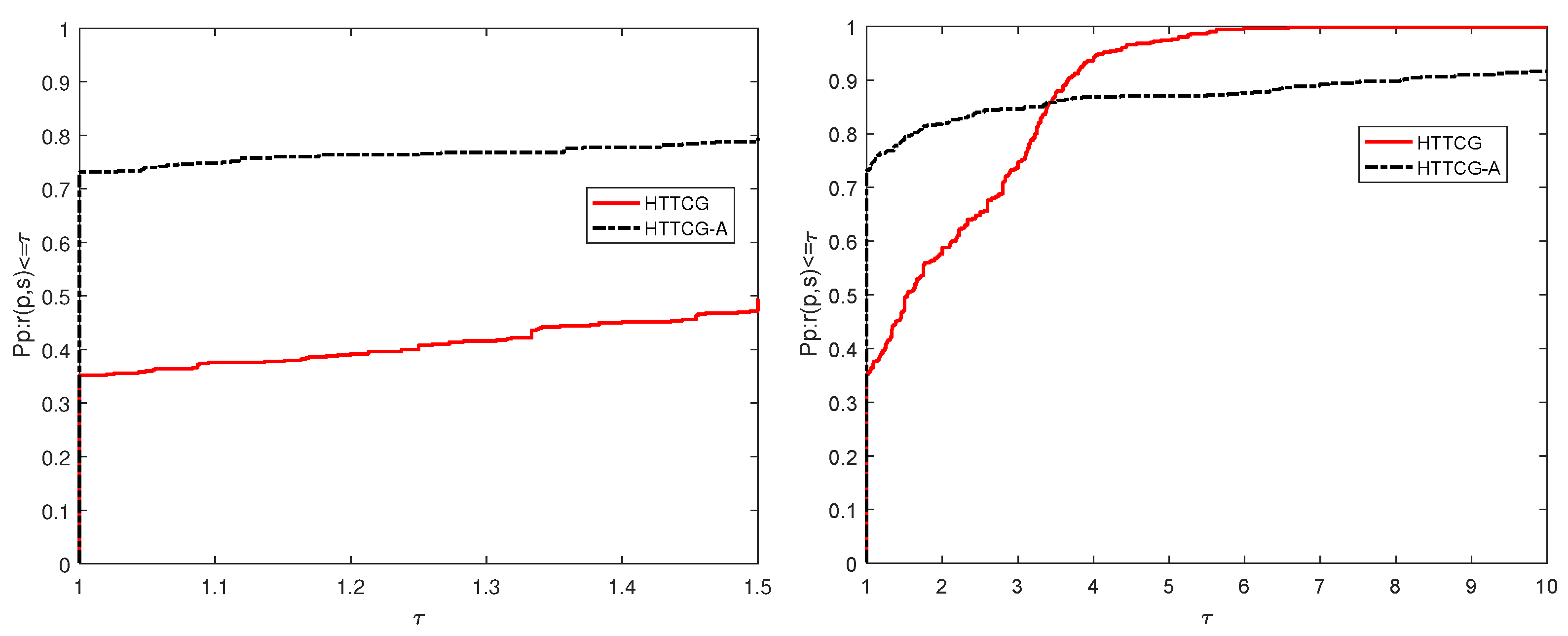
4.2. Accelerated Strategy for Algorithm 2

In order to improve the numerical performances of Algorithm 2, in this subsection, we utilize the acceleration strategy in [40], which modifies the step in a multiplicative manner along iterations. Concretely, the iterative form (2) reduces to:

$$x_{k+1}=x_k+{\rho }_k{\alpha }_k{d}_k,$$

(35)

where ${\theta }_k={\alpha }_k{g}_k^T{d}_k$ and ${\xi }_k={\alpha }_k{[g(x_k+{\alpha }_k{d}_k)-g_k]}^T{d}_k$ and if ${\xi }_k<0$, ${\rho }_k=\frac{{\theta }_k}{{\xi }_k}$, otherwise, ${\rho }_k=1$.

We also test the problems in Table 1 and compare Algorithm 2 with the acceleration strategy with Algorithm 2. The corresponding parameters remain unchanged. The performance profiles can be founded in Figure 4, Figure 5 and Figure 6.

From Figure 4, we find that the Algorithm 2 with the acceleration strategy (HTTCG-A method) in $73\%$ and HTTCG method in $36\%$ solve the testing problems with the least iteration number. From Figure 5, we see that the HTTCG-A method in $72\%$ and HTTCG method in $35\%$ solve the testing problems with the least number of computing functions and gradient. From Figure 6, we see that the HTTCG-A method in $59\%$ and HTTCG method in $28\%$ solve the testing problems with the least CPU time consumed. These all indicate that the acceleration strategy works and can reduce the number of iterations, the number of computing functions and gradients and the time consumed.

5. Conclusions

Unconstrained smooth optimization problems can be found in many problems such as optimal control problems and machine learning problems, etc. In this paper, a hybrid three-term descent conjugate gradient algorithm is proposed. This hybrid three-term conjugate gradient algorithm owns the sufficient descent property independent of any line search technique. Meanwhile, it also satisfies the extent Dai–Liao conjugate condition. Under some mild conditions, this algorithm is globally convergent for the uniformly convex functions. For general nonlinear function, the hybrid method is also globally convergent by using some modified secant conditions. Numerical results indicate that the hybrid method is effective and reliable. Meanwhile, an acceleration strategy is adopted to improve the numerical performances. In the future, we will apply our conjugate gradient methods to some non-smooth problems by smoothing strategy and Moreau–Yosida regularization technique and to image restoration problems.

References

1. Fan, J.; Zeng, J. A Levenberg–Marquardt algorithm with correction for singular system of nonlinear equations. Appl. Math. Comput. 2013, 219, 9438–9446. [Google Scholar] [CrossRef]
2. Yerina, M.; Izmailov, A. The Gauss–Newton method for finding singular solutions to systems of nonlinear equations. Comp. Math. Math. Phys. 2007, 47, 748–759. [Google Scholar] [CrossRef]
3. Yuan, G.; Wei, Z.; Wang, Z. Gradient trust region algorithm with limited memory BFGS update for nonsmooth convex minimization. Comput. Optim. Appl. 2013, 54, 45–64. [Google Scholar] [CrossRef]
4. Yuan, G.; Wei, Z.; Lu, X. Global convergence of BFGS and PRP methods under a modified weak Wolfe–Powell line search. Appl. Math. Model. 2017, 47, 811–825. [Google Scholar] [CrossRef]
5. Yuan, G.; Lu, J.; Wang, Z. The PRP conjugate gradient algorithm with a modified WWP line search and its application in the image restoration problems. Appl. Numer. Math. 2020, 152, 1–11. [Google Scholar] [CrossRef]
6. Dai, Y.; Han, J.; Liu, G.; Sun, D.; Yin, H.; Yuan, Y. Convergence properties of nonlinear conjugate gradient methods. SIAM J. Optim. 2000, 10, 345–358. [Google Scholar] [CrossRef]
7. Yuan, G.; Wang, X.; Sheng, Z. Family weak conjugate gradient algorithms and their convergence analysis for nonconvex functions. Numer. Algorithms 2020, 84, 935–956. [Google Scholar] [CrossRef]
8. Hager, W.; Zhang, H. A survey of nonlinear conjugate gradient methods. Pac. J. Optim. 2006, 2, 35–58. [Google Scholar]
9. Andrei, N. Numerical comparison of conjugate gradient algorithms for unconstrained optimization. Stud. Inform. Control. 2007, 16, 333–352. [Google Scholar]
10. Li, X.; Wang, X.; Sheng, Z.; Duan, X. A modified conjugate gradient algorithm with backtracking line search technique for large-scale nonlinear equations. Int. J. Comput. Math. 2018, 95, 382–395. [Google Scholar] [CrossRef]
11. Wang, X.; Hu, W.; Yuan, G. A Modified Wei-Yao-Liu Conjugate Gradient Algorithm for Two Type Minimization Optimization Models; Springer: Cham, Switzerland, 2018. [Google Scholar]
12. Yuan, G.; Meng, Z.; Li, Y. A modified Hestenes and Stiefel conjugate gradient algorithm for large-scale nonsmooth minimizations and nonlinear equations. J. Optim. Theory Appl. 2016, 168, 129–152. [Google Scholar] [CrossRef]
13. Cao, J.; Wu, J. A conjugate gradient algorithm and its applications in image restoration. Appl. Numer. Math. 2020, 152, 243–252. [Google Scholar] [CrossRef]
14. Møller, F. A scaled conjugate gradient algorithm for fast supervised learning. Neural Netw. 1993, 6, 525–533. [Google Scholar]
15. Zhou, Y.; Wu, Y.; Li, X. A New Hybrid PRPFR Conjugate Gradient Method for Solving Nonlinear Monotone Equations and Image Restoration Problems. Math. Probl. Eng. 2020, 2020, 1–13. [Google Scholar] [CrossRef]
16. Hestenes, R.; Stiefel, L. Methods of conjugate gradients for solving linear systems. J. Res. Natl. Bur. Stand. 1952, 49, 409–436. [Google Scholar] [CrossRef]
17. Fletcher, R.; Reeves, C.M. Function minimization by conjugate gradients. Comput. J. 1964, 2, 149–154. [Google Scholar] [CrossRef] [Green Version]
18. Dai, Y.; Liao, L. New conjugacy conditions and related nonlinear conjugate gradient methods. Appl. Math. Opt. 2001, 43, 87–101. [Google Scholar] [CrossRef]
19. Polak, E. The conjugate gradient method in extreme problems. USSR Comput. Math. Math. Phys. 1969, 9, 94–112. [Google Scholar] [CrossRef]
20. Polak, E.; Ribière, G. Note sur la convergence de directions conjugees. Rev. Fr. Informat Rech. Opertionelle 1969, 16, 35–43. [Google Scholar]
21. Zhang, K.; Liu, H.; Liu, Z. A new Dai-Liao conjugate gradient method with optimal parameter choice. Numer. Funct. Anal. Optim. 2019, 40, 194–215. [Google Scholar] [CrossRef]
22. Andrei, N. A Dai-Liao conjugate gradient algorithm with clustering of eigenvalues. Numer. Algorithms 2018, 77, 1273–1282. [Google Scholar] [CrossRef]
23. Babaie-kafaki, S.; Ghanbari, R. The Dai-Liao nonlinear conjugate gradient method with optimal parameter choices. Eur. J. Oper. Res. 2014, 234, 625–630. [Google Scholar] [CrossRef]
24. Zheng, Y.; Zheng, B. Two new Dai-Liao-type conjugate gradient methods for unconstrained optimization problems. J. Optim. Theory Appl. 2017, 175, 502–509. [Google Scholar] [CrossRef]
25. Peyghami, M.; Ahmadzadeh, H.; Fazli, A. A new class of efficient and globally convergent conjugate gradient methods in the Dai-Liao family. Optim. Method. Softw. 2015, 30, 843–863. [Google Scholar] [CrossRef]
26. Yuan, G.; Wang, X.; Sheng, Z. The projection technique for two open problems of unconstrained optimization problems. J. Optim. Theory Appl. 2020, 186, 590–619. [Google Scholar] [CrossRef]
27. Narushima, Y.; Yabe, H.; Ford, J. A three-term conjugate gradient method with sufficient descent property for unconstrained optimization. SIAM J. Optim. 2011, 21, 212–230. [Google Scholar] [CrossRef] [Green Version]
28. Zhang, L.; Zhou, W.; Li, D. Some descent three-term conjugate gradient methods and their global convergence. Optim. Method. Softw. 2007, 22, 697–711. [Google Scholar] [CrossRef]
29. Zhang, L.; Zhou, W.; Li, D. A descent modified Polak-Ribière-Polyak conjugate gradient method and its global convergence. IMA J. Numer. Anal. 2006, 26, 629–640. [Google Scholar] [CrossRef]
30. Andrei, N. A simple three-term conjugate gradient algorithm for unconstrained optimization. J. Comput. Appl. Math. 2013, 241, 19–29. [Google Scholar] [CrossRef]
31. Babaie-Kafaki, S.; Ghanbari, R. Two modified three-term conjugate gradient methods with sufficient descent property. Optim. Lett. 2014, 8, 2285–2297. [Google Scholar] [CrossRef]
32. Li, D.; Fukushima, M. A modified BFGS method and its global convergence in nonconvex minimization. J. Comput. Appl. Math. 2001, 129, 15–35. [Google Scholar] [CrossRef] [Green Version]
33. Zhang, L. A derivative-free conjugate residual method using secant condition for general large-scale nonlinear equations. Numer. Algorithms 2020, 83, 1277–1293. [Google Scholar] [CrossRef]
34. Sugiki, K.; Narushima, Y.; Yabe, H. Globally convergent three-term conjugate gradient methods that use secant conditions and generate descent search directions for unconstrained optimization. J. Optim. Theory Appl. 2012, 153, 733–757. [Google Scholar] [CrossRef]
35. Wei, Z.; Li, G.; Qi, L. New quasi-Newton methods for unconstrained optimization problems. Appl. Math. Comput. 2006, 175, 1156–1188. [Google Scholar] [CrossRef]
36. Yuan, G.; Wei, Z. Convergence analysis of a modified BFGS method on convex minimizations. Comput. Optim. Appl. 2010, 47, 237–255. [Google Scholar] [CrossRef]
37. Dai, Y.; Kou, C. A nonlinear conjugate gradient algorithm with an optimal property and an improved wolfe line search. SIAM J. Optim. 2013, 23, 296–320. [Google Scholar] [CrossRef] [Green Version]
38. Andrei, N. An unconstrained optimization test functions collection. Adv. Model Optim. 2008, 10, 147–161. [Google Scholar]
39. Dolan, E.; Moré, J. Benchmarking optimization software with performance profiles. Math. Program 2002, 91, 201–213. [Google Scholar] [CrossRef]
40. Andrei, N. An acceleration of gradient descent algorithm with backtracking for unconstrained optimization. Numer. Algorithms 2006, 42, 63–73. [Google Scholar] [CrossRef]
Figure 1. Performance profiles of the numerical results for these methods in number of iterations case.
Mathematics 09 01353 g001
Figure 2. Performance profiles of the numerical results for these methods in a number of function and gradient evaluations.
Mathematics 09 01353 g002
Figure 3. Performance profiles of the numerical results for these methods in CPU time consumed case.
Mathematics 09 01353 g003
Figure 4. Performance profiles of Algorithm 2 and the acceleration form in NI case.
Mathematics 09 01353 g004
Figure 5. Performance profiles of Algorithm 2 and the acceleration form in NFG case.
Mathematics 09 01353 g005
Figure 6. Performance profiles of Algorithm 2 and the acceleration form in CPU Time case.
Mathematics 09 01353 g006