
An Improved Slime Mould Algorithm for Demand Estimation of Urban Water Resources

Abstract
1. Introduction
2. An Improved Slime Mould Algorithm
2.1. Slime Mould Algorithm
2.1.1. Initialization
2.1.2. Approach Food
2.1.3. Wrap Food
| Algorithm 1. Slime mould algorithm |
| Input: Slime mould population Xi (i = 1,2,…,n) and related parameters such as n, dim, max_t; |
| Output: Optimal fitness value best_fitness and the corresponding optimal position Xb. |
| While (t < max_t) |
| Check if solutions go outside the search space and bring them back |
| Calculate fitness values of all individuals, update the best and worst fitness value |
| Calculate the weight W according to Equation (6) |
| Record the best fitness best_fitness and the corresponding Xb |
| For each search agent |
| Update the value of vb, vc, and p |
| Update the individual position according to Equation (8) |
| End For |
| t = t + 1 |
| End While |
2.2. The Proposed Improved Slime Mould Algorithm
2.2.1. Opposition-Based Learning
2.2.2. Elite Chaotic Searching Strategy
2.2.3. The Improved Slime Mould Algorithm Combining the Two Strategies
| Algorithm 2. Pseudo-code of the ESMA |
| Initialize related parameters such asn, dim, max_t, and Slime mould populationXi (i = 1,2,...,n); |
| Calculate opposition population of current population Xi (i = 1,2,…,n) by Equation (9) |
| Calculate the fitness of population , pick n individuals with better fitness value as the current population |
| While (t < max_t) |
| Calculate fitness values of all individuals, update the best and worst fitness value |
| Calculate the weight W according to Equation (6) |
| Record the best fitness best_fitness and the corresponding Xb |
| For i = 1: n |
| Update the value of vb, vc, and p |
| Update the population position according to Equation (8) |
| End For |
| Calculate by Equation (9), pick n individuals with better fitness value as the current population based on the fitness values of population |
| Select the first m individuals as elite individuals EXi |
| Calculate new elite individuals obtained by chaotic iteration through Equations (10)–(13) |
| Update the elite individuals’ position according to Equation (14) |
| Check if solutions go outside the search space and bring them back |
| t = t + 1 |
| End While |
| Return optimal fitness value best_fitness and the corresponding optimal position Xb |
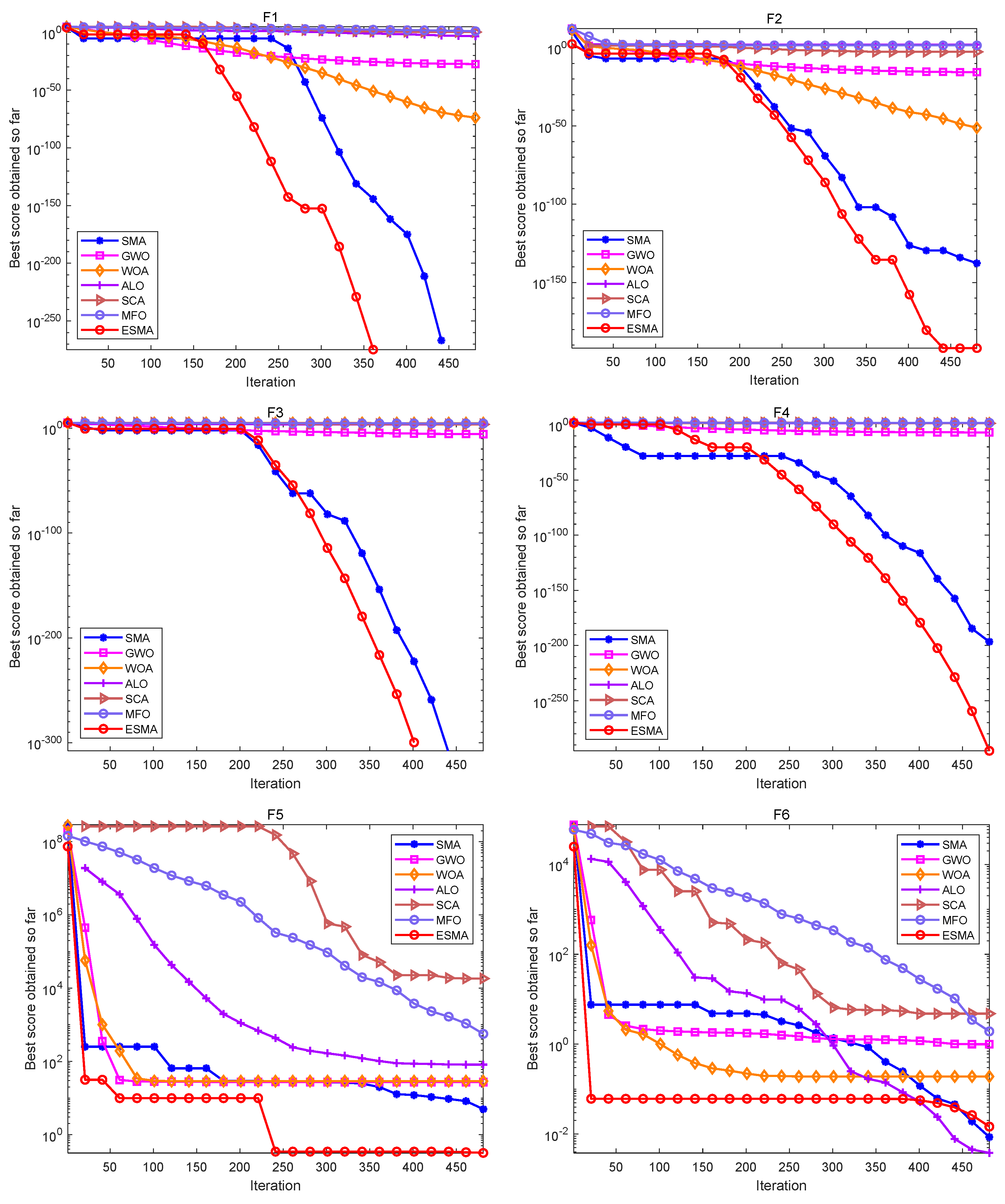
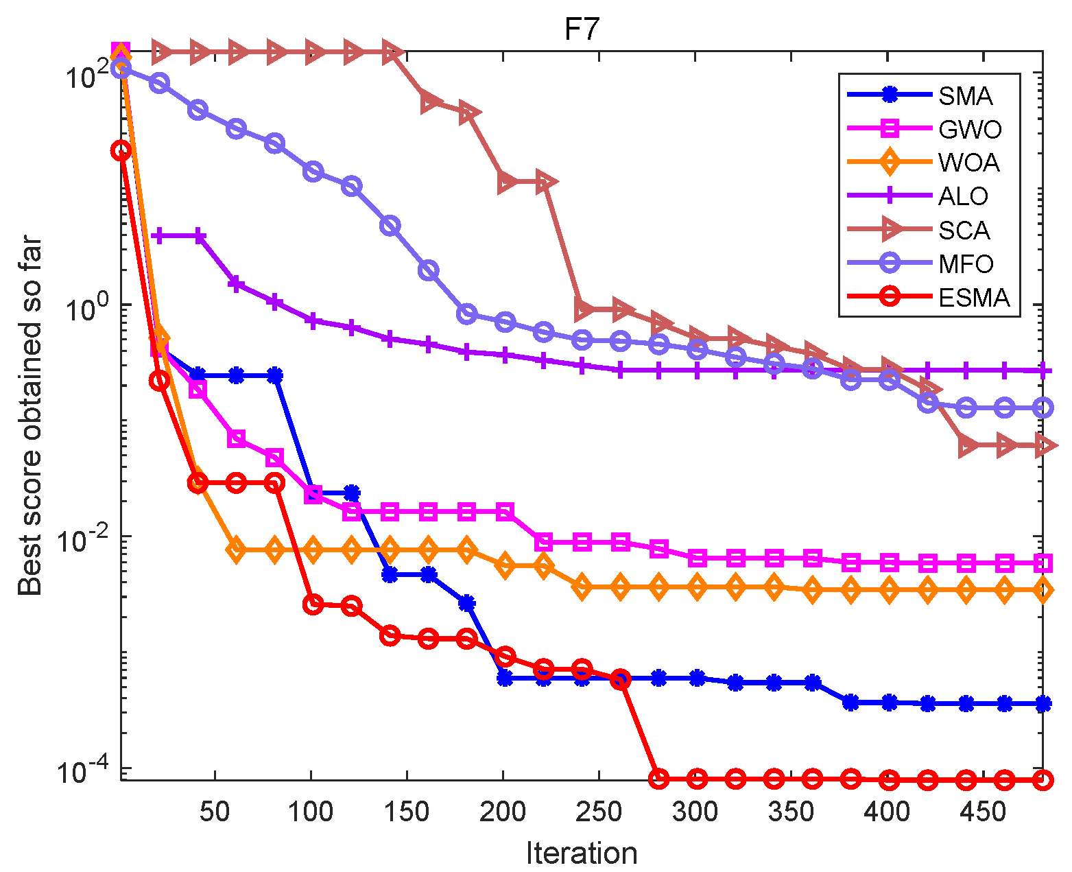
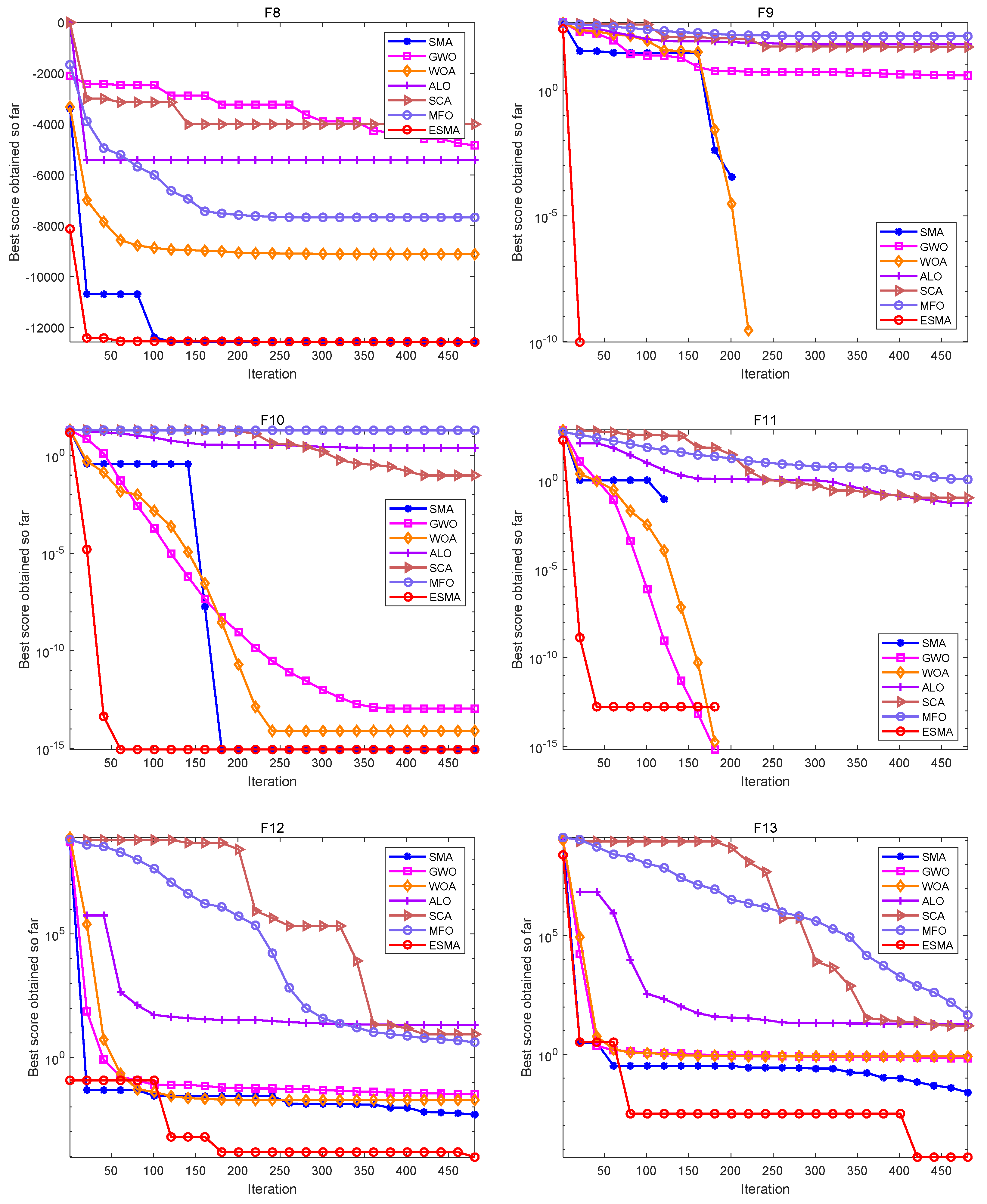
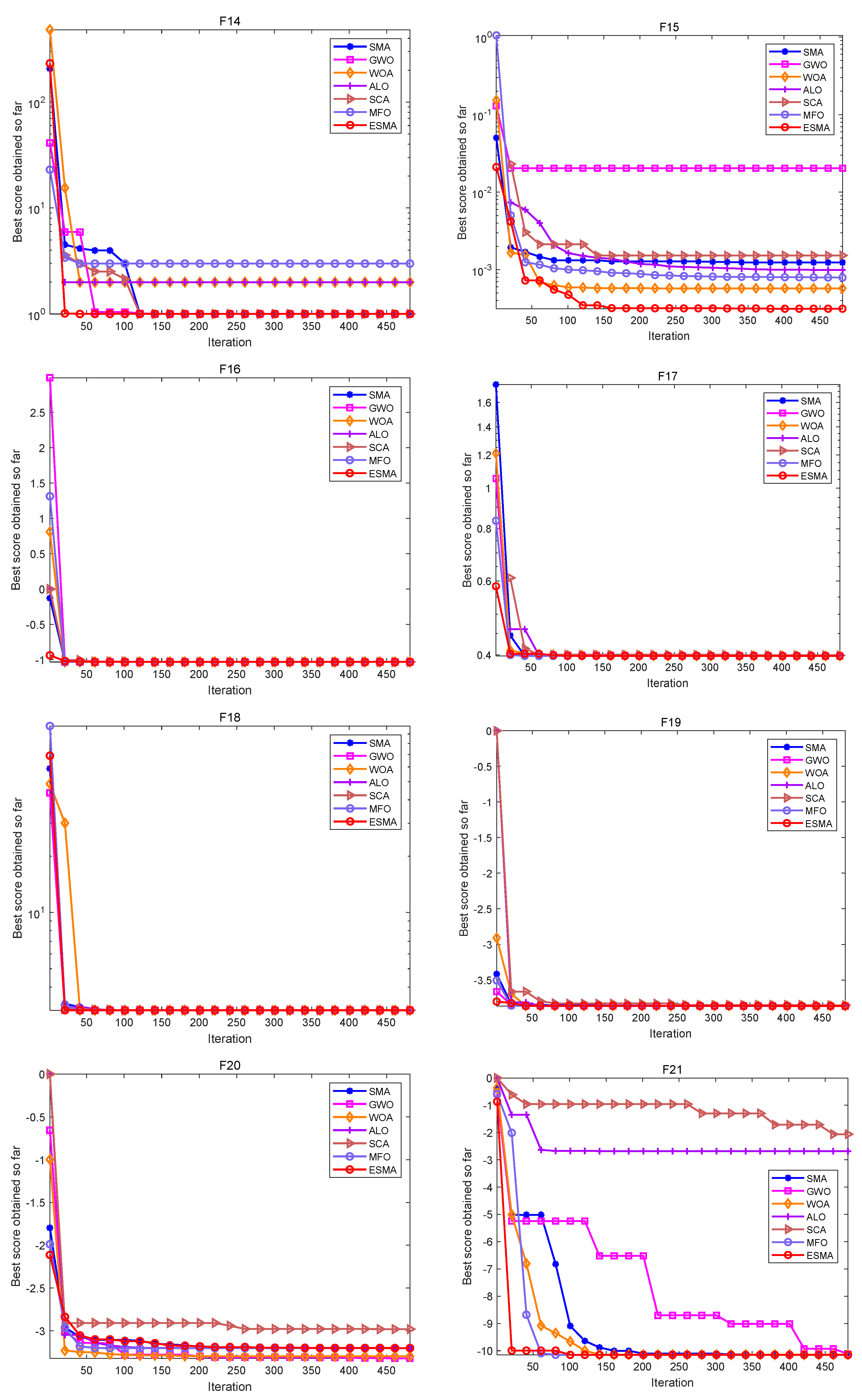
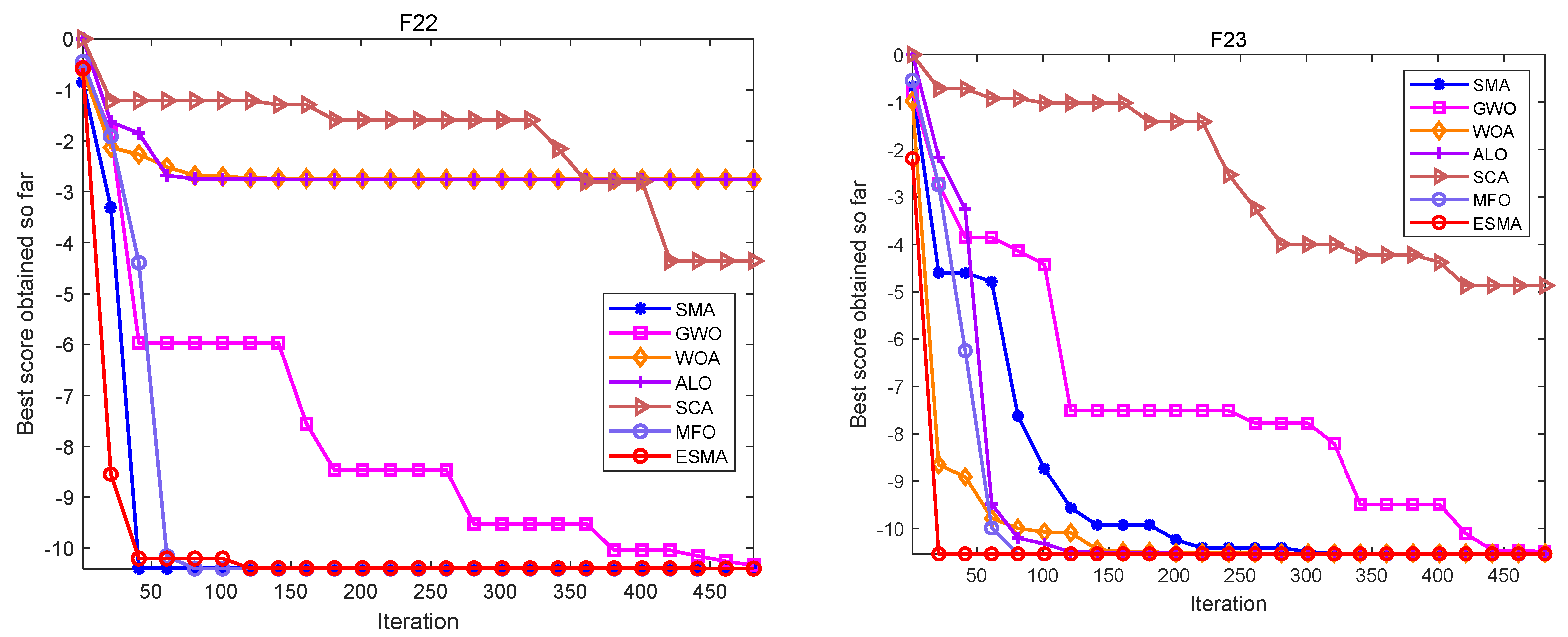
3. Comparison of the ESMA with Other Algorithms
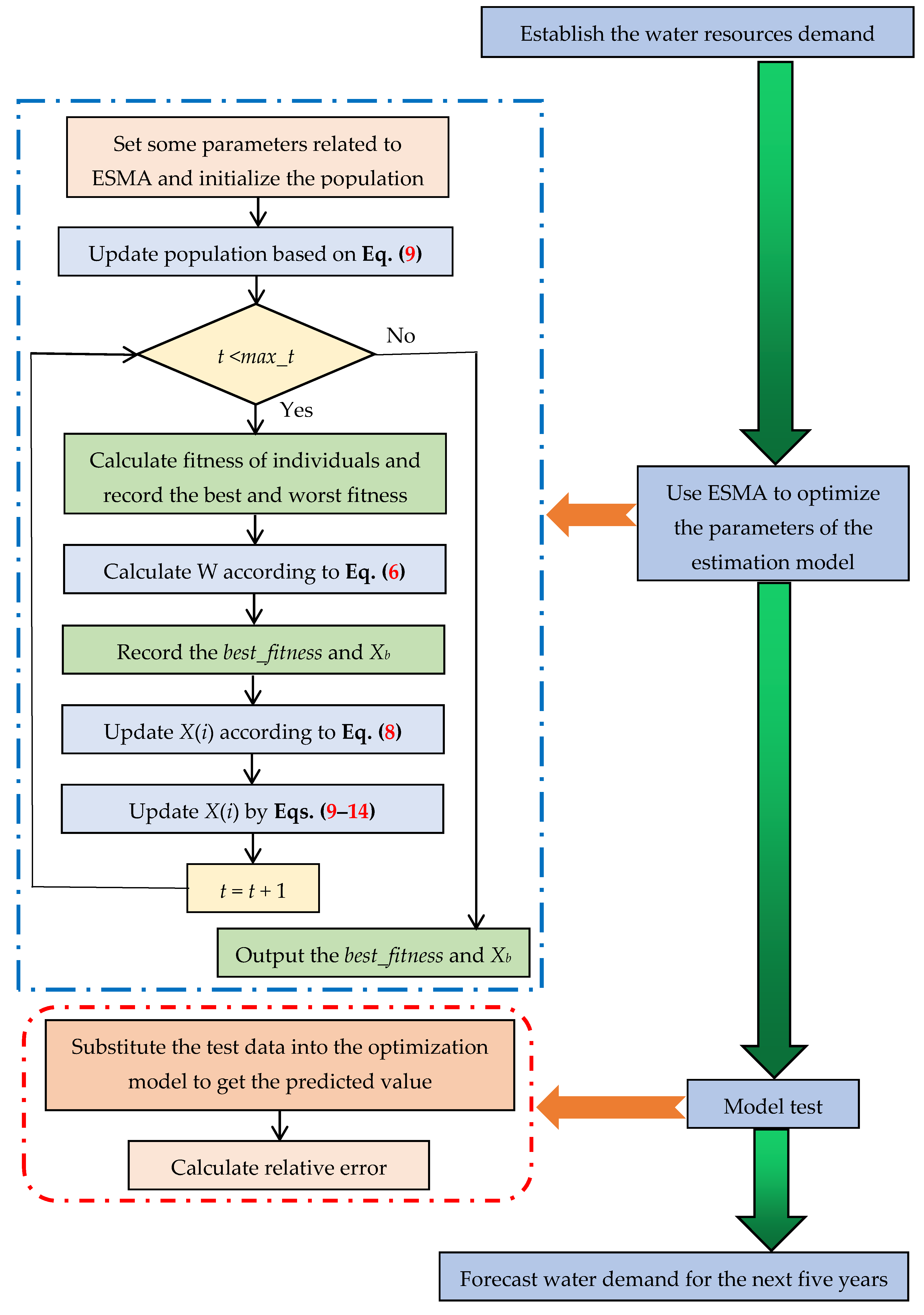
4. The ESMA for Demand Estimation of Water Resources
4.1. Establishment of Water Resources Demand Estimation Model
4.2. Optimization of Water Resources Demand Estimation Model
4.3. The ESMA Solves the Parameters of Water Demand Estimation Model
4.4. The Experiment and Analysis of Water Resources Demand Estimation Model
4.4.1. Data Preprocessing
4.4.2. Algorithm Parameters Setting
4.4.3. Performance Evaluation Criteria of the Algorithms
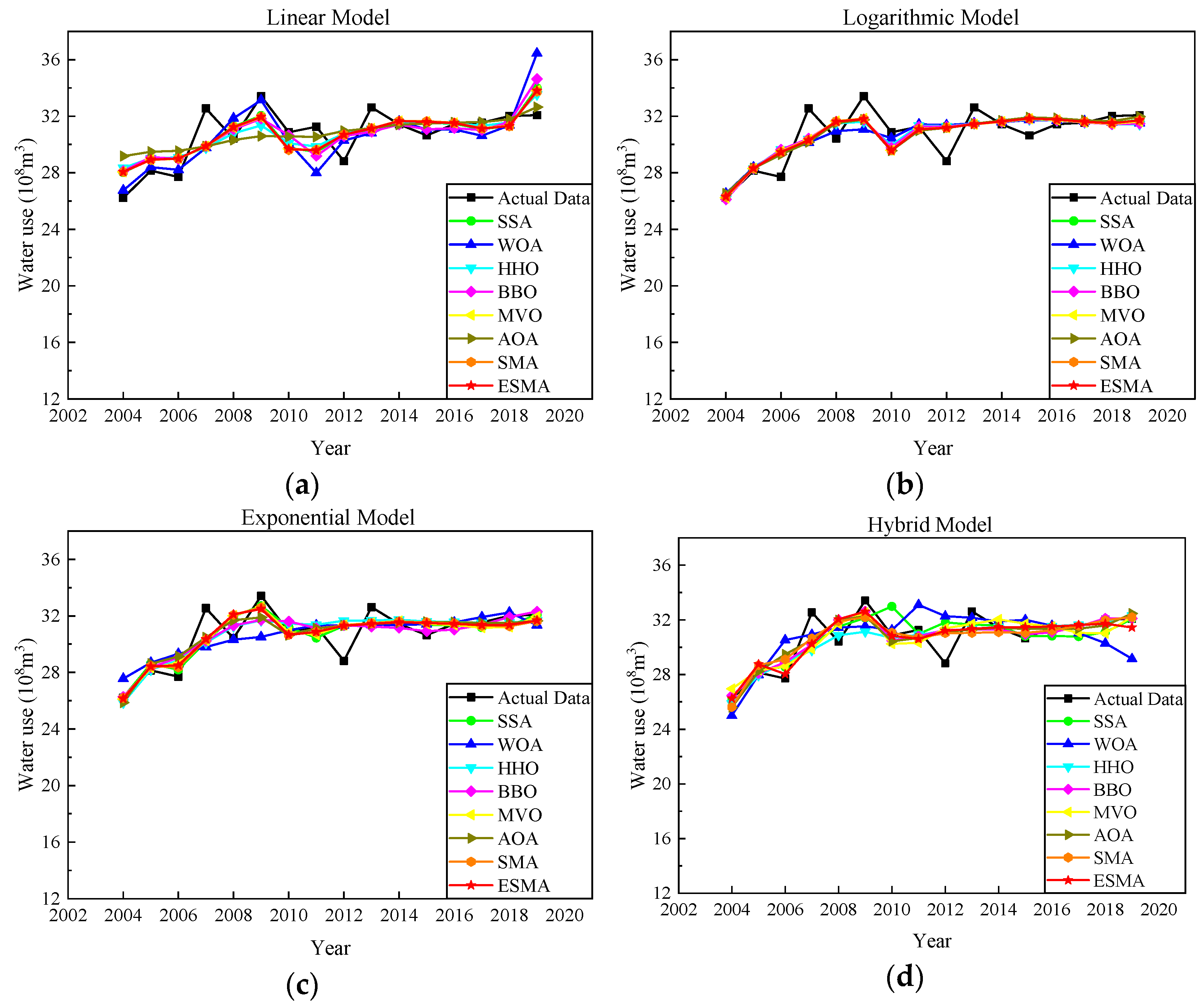
4.4.4. Result and Analysis
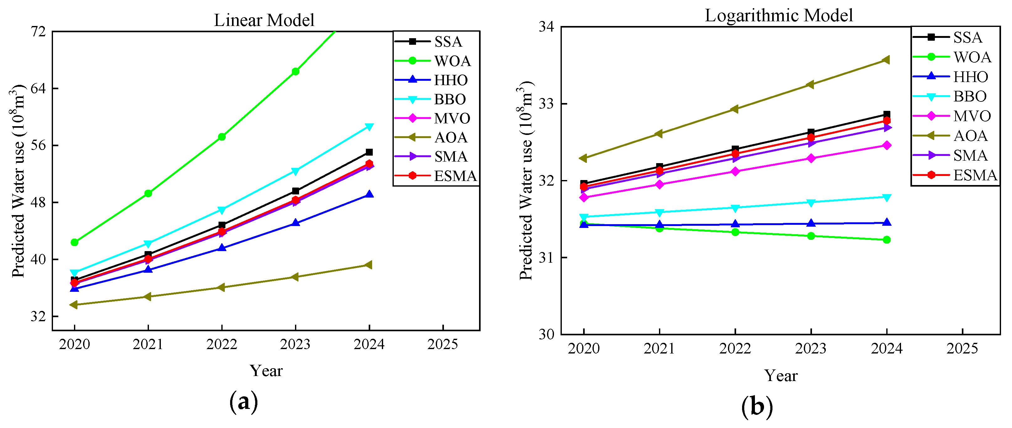
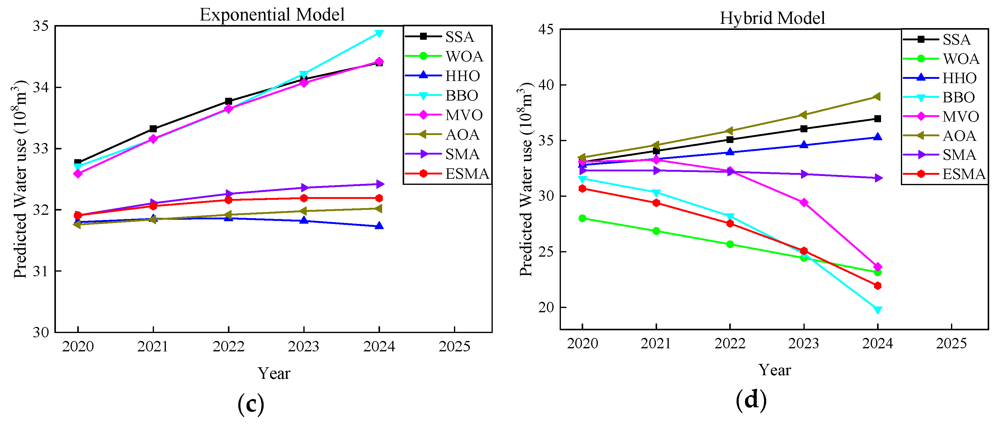
4.5. Forecast of Water Resources Demand for 2020–2024
5. Conclusions
Author Contributions
Funding
Institutional Review Board Statement
Informed Consent Statement
Data Availability Statement
Conflicts of Interest
References
- Davijani, M.H.; Banihabib, M.E.; Anvar, A.N.; Hashemi, S.R. Optimization model for the allocation of water resources based on the maximization of employment in the agriculture and industry sectors. J. Hydrol. 2016, 533, 430–438. [Google Scholar] [CrossRef]
- Arbués, F.; García-Valiñas, M.Á.; Martínez-Espiñeira, R. Estimation of residential water demand: A state-of-the-art review. J. Soc. Econ. 2003, 32, 81–102. [Google Scholar] [CrossRef]
- Hang, L.; Chi, Z.; Dong, M.; Ming, Z. Water demand prediction of Grey Markov model based on GM(1,1). In Proceedings of the 2016 3rd International Conference on Mechatronics and Information Technology, Shenzhen, China, 9–10 April 2016. [Google Scholar]
- Brentan, B.M.; Luvizotto, E., Jr.; Herrera, M.; Lzquierdo, J.; Pérez-García, R. Hybrid regression model for near real-time urban water demand forecasting. J. Comput. Appl. Math. 2017, 309, 532–541. [Google Scholar] [CrossRef]
- Al-Zahrani, M.A.; Abo-Monasar, A. Urban Residential Water Demand Prediction Based on Artificial Neural Networks and Time Series Models. Water Resour. Manag. 2015, 29, 3651–3662. [Google Scholar] [CrossRef]
- Bai, Y.; Wang, P.; Li, C.; Xie, J.J.; Wang, Y. A multi-scale relevance vector regression approach for daily urban water demand forecasting. J. Hydrol. 2014, 517, 236–245. [Google Scholar] [CrossRef]
- Pulido-Calvo, I.; Gutiérrez-Estrada, J.C. Improved irrigation water demand forecasting using a soft-computing hybrid model. Biosyst. Eng. 2009, 102, 202–218. [Google Scholar] [CrossRef]
- Romano, M.; Kapelan, Z. Adaptive water demand forecasting for near real-time management of smart water distribution systems. Environ. Modell. Softw. 2014, 60, 265–276. [Google Scholar] [CrossRef]
- Oliveira, P.J.; Steffen, J.L.; Cheung, P. Parameter estimation of seasonal arima models for water demand forecasting using the harmony search algorithm. Procedia Eng. 2017, 186, 177–185. [Google Scholar] [CrossRef]
- Kennedy, J.; Eberhart, R.C. Particle swarm optimization. In Proceedings of the IEEE International Conference on Neural Networks, Perth, WA, Australia, 27 November–1 December 1995; pp. 1942–1948. [Google Scholar]
- Mirjalili, S.; Lewis, A. The whale optimization algorithm. Adv. Eng. Soft. 2016, 95, 51–67. [Google Scholar] [CrossRef]
- Mirjalili, S.; Mirjalili, S.M.; Lewis, A. Grey wolf optimizer. Adv. Eng. Soft. 2014, 69, 46–61. [Google Scholar] [CrossRef]
- Heidari, A.; Mirjalili, S.; Farris, H.; Aljarah, I.; Mafarja, M.; Chen, H. Harris hawks optimization: Algorithm and applications. Future Gener. Comput. Syst. 2019, 97, 849–872. [Google Scholar] [CrossRef]
- Yang, X.S. Firefly algorithm, stochastic test functions and design optimization. Int. J. Bio Inspir. Comput. 2010, 2, 78–84. [Google Scholar] [CrossRef]
- Zhao, W.G.; Zhang, Z.X.; Wang, L.Y. Manta ray foraging optimization: An effective bio-inspired optimizer for engineering applications. Eng. Appl. Artif. Intell. 2020, 87, 103300. [Google Scholar] [CrossRef]
- Faramarzi, A.; Heidarinejad, M.; Mirjalil, S.; Gandomi, A.H. Marine Predators Algorithm: A nature-inspired metaheuristic. Expert Syst. Appl. 2020, 152, 113377. [Google Scholar] [CrossRef]
- Li, S.M.; Chen, H.L.; Wang, M.J.; Heidari, A.A.; Mirjalili, S. Slime mould algorithm: A new method for stochastic optimization. Future Gener. Comput. Syst. 2020, 111, 300–323. [Google Scholar] [CrossRef]
- Vashishtha, G.; Chauhan, S.; Singh, M.; Kumar, R. Bearing defect identification by swarm decomposition considering permutation entropy measure and opposition-based slime mould algorithm. Measurement 2021, 178, 109389. [Google Scholar] [CrossRef]
- Mostafa, M.; Rezk, H.; Aly, M.; Ahmed, E.M. A new strategy based on slime mould algorithm to extract the optimal model parameters of solar PV panel. Sustain. Energy Techn. 2020, 42, 100849. [Google Scholar] [CrossRef]
- Abdel-Basset, M.; Mohamed, R.; Chakrabortty, R.K.; Ryan, M.J.; Mirjalili, S. An efficient binary slime mould algorithm integrated with a novel attacking-feeding strategy for feature selection. Comput. Ind. Eng. 2021, 153, 107078. [Google Scholar] [CrossRef]
- Kumar, C.; Raj, T.D.; Premkumar, M.; Raj, T.D. A new stochastic slime mould optimization algorithm for the estimation of solar photovoltaic cell parameters. Optik 2020, 223, 165277. [Google Scholar] [CrossRef]
- Rizk-Allah, R.M.; Hassanien, A.E.; Song, D.R. Chaos-opposition-enhanced slime mould algorithm for minimizing the cost of energy for the wind turbines on high-altitude sites. ISA Trans. 2021, in press. [Google Scholar] [CrossRef]
- Abdel-Basset, M.; Chang, V.; Mohamed, R. HSMA_WOA: A hybrid novel Slime mould algorithm with whale optimization algorithm for tackling the image segmentation problem of chest X-ray images. Appl. Soft Comput. 2020, 95, 106642. [Google Scholar] [CrossRef]
- Houssein, E.H.; Mahdy, M.A.; Blondin, M.J.; Shebl, D.; Mohamed, W.M. Hybrid slime mould algorithm with adaptive guided differential evolution algorithm for combinatorial and global optimization problems. Expert Syst. Appl. 2021, 174, 114689. [Google Scholar] [CrossRef]
- Djekidel, R.; Bentouati, B.; Javaid, M.S.; Bouchekara, H.R.E.H.; Bayoumi, A.S.; El-Sehiemy, R.A. Mitigating the effects of magnetic coupling between HV Transmission Line and Metallic Pipeline using Slime Mould Algorithm. J. Magn. Magn. Mater. 2021, 529, 167865. [Google Scholar] [CrossRef]
- El-Fergany, A.A. Parameters identification of PV model using improved slime mould optimizer and Lambert W-function. Energy Rep. 2021, 7, 875–887. [Google Scholar] [CrossRef]
- Tizhoosh, R.H. Opposition-based learning: A new scheme for machine intelligence. In Proceedings of the International Conference on Computational Intelligence for Modelling, Control & Automation and International Conference on Intelligent Agents, Vienna, Austria, 28–30 November 2005; pp. 695–701. [Google Scholar]
- Muthusamy, H.; Ravindran, S.; Yaacob, S.; Polat, K. An improved elephant herding optimization using sine-cosine mechanism and opposition based learning for global optimization problems. Expert Syst. Appl. 2021, 172, 114607. [Google Scholar] [CrossRef]
- Mirjalili, S. The ant lion optimizer. Adv. Eng. Soft. 2015, 83, 80–98. [Google Scholar] [CrossRef]
- Mirjalili, S. SCA: A Sine Cosine Algorithm for solving optimization problems. Knowl. Based Syst. 2016, 96, 120–133. [Google Scholar] [CrossRef]
- Mirjalili, S. Moth-flame optimization algorithm: A novel nature-inspired heuristic paradigm. Knowl. Based Syst. 2015, 89, 228–249. [Google Scholar] [CrossRef]
- Mirjalili, S.; Gandomi, A.H.; Mirjalili, S.Z.; Saremi, S.; Faris, H.; Mirjalili, S.M. Salp swarm algorithm: A bio-inspired optimizer for engineering design problems. Adv. Eng. Soft. 2017, 114, 163–191. [Google Scholar] [CrossRef]
- Xing, B.; Gao, W.J. Biogeography—Based Optimization Algorithm; Springer: Berlin/Heidelberg, Germany, 2014. [Google Scholar]
- Mirjalili, S.; Mirjalili, S.M.; Hatamlou, A. Multi-Verse Optimizer: A nature-inspired algorithm for global optimization. Neural Comput. Appl. 2015, 27, 495–513. [Google Scholar] [CrossRef]
- Hashim, F.A.; Hussain, K.; Houssein, E.H.; Mai, S.M.; Ai-Atabany, W. Archimedes optimization algorithm: A new metaheuristic algorithm for solving optimization problems. Appl. Intell. 2021, 51, 1531–1551. [Google Scholar] [CrossRef]


| Algorithm | Parameter Value | Popsize | Iterations of Number |
|---|---|---|---|
| SMA | z = 0.03 | 30 | 500 |
| ESMA | z = 0.03, selected elite proportion pr = 0.1 | 30 | 500 |
| GWO | Component of coefficient vectors: = [2, 0] | 30 | 500 |
| WOA | value of coefficient vectors : = [2, 0] | 30 | 500 |
| ALO | NA | 30 | 500 |
| SCA | The value of constant = 2 | 30 | 500 |
| MFO | b = 1 | 30 | 500 |
| Classification | Name | Detailed Settings |
|---|---|---|
| Hardware | CPU | Intel(R) Core(TM) i5-8625U |
| Frequency | 1.60 GHz 1.80 GHz | |
| RAM | 8.00 GB | |
| Hard drive | 512 GB | |
| Software | Operating system | Windows 10 |
| Language | MATLAB R2018a |
| Function | D | Range | fopt |
|---|---|---|---|
| 30 | [−100, 100]n | 0 | |
| 30 | [−10, 10]n | 0 | |
| 30 | [−100, 100]n | 0 | |
| 30 | [−100, 100]n | 0 | |
| 30 | [−30, 30]n | 0 | |
| 30 | [−100, 100]n | 0 | |
| 30 | [−1.28, 1.28]n | 0 |
| Function | D | Range | fopt |
|---|---|---|---|
| 30 | [−500, 500]n | −12,569.5 | |
| 30 | [−5.12, 5.12]n | 0 | |
| 30 | [−32, 32]n | 0 | |
| 30 | [−600, 600]n | 0 | |
| 30 | [−50, 50]n | 0 | |
| 30 | [−50, 50]n | 0 |
| Function | D | Range | fopt |
|---|---|---|---|
| 2 | [−65.536, 65.536]n | 0.998 | |
| 4 | [−5, 5]n | 3.075 × 10⁻⁴ | |
| 2 | [−5, 5]n | −1.0316 | |
| 2 | [−5, 5]n | 0.398 | |
| 2 | [−2, 2]n | 3 | |
| 3 | [0, 1]n | −3.86 | |
| 6 | [0, 1]n | −3.322 | |
| 4 | [0, 10]n | −10.1532 | |
| 4 | [0, 10]n | −10.4028 | |
| 4 | [0, 10]n | −10.5363 |
| Algorithms | ||||||||
|---|---|---|---|---|---|---|---|---|
| GWO | WOA | ALO | SCA | MFO | SMA | ESMA | ||
| F1 | Best | 4.31E-29 | 7.16E-82 | 2.00E-4 | 4.41E-3 | 7.01E-1 | 0 | 0 |
| Worst | 6.38E-27 | 7.28E-75 | 5.01E-3 | 4.52E+1 | 2.00E+4 | 0 | 0 | |
| Mean | 1.48E-27 | 9.44E-76 | 1.57E-3 | 1.09E+1 | 3.03E+3 | 0 | 0 | |
| Std | 2.01E-27 | 1.84E-75 | 1.21E-3 | 1.32E+1 | 5.70E+3 | 0 | 0 | |
| Rank | 3 | 2 | 4 | 5 | 6 | 1 | 1 | |
| F2 | Best | 3.37E-17 | 2.71E-55 | 2.3137 | 7.20E-6 | 4.07E-1 | 1.54E-284 | 0 |
| Worst | 4.36E-16 | 3.54E-50 | 1.20E+2 | 6.19E-2 | 8.00E+1 | 3.58E-151 | 0 | |
| Mean | 1.31E-16 | 1.87E-51 | 4.73E+1 | 1.23E-2 | 3.04E+1 | 1.79E-152 | 0 | |
| Std | 1.09E-16 | 7.88E-51 | 4.72E+1 | 1.78E-2 | 2.44E+1 | 8.04E-152 | 0 | |
| Rank | 4 | 3 | 7 | 5 | 6 | 2 | 1 | |
| F3 | Best | 2.84E-9 | 1.49E+4 | 1.22E+3 | 2.74E+3 | 1.72E+3 | 0 | 0 |
| Worst | 5.78E-4 | 5.90E+4 | 9.89E+3 | 2.28E+4 | 5.39E+4 | 6.47E-295 | 0 | |
| Mean | 3.37E-5 | 3.75E+4 | 4.12E+3 | 9.45E+3 | 2.08E+4 | 3.24E-296 | 0 | |
| Std | 1.28E-4 | 1.07E+4 | 2.03E+3 | 5.15E+3 | 1.25E+4 | 0 | 0 | |
| Rank | 3 | 7 | 4 | 5 | 6 | 2 | 1 | |
| F4 | Best | 9.21E-8 | 1.6832 | 7.3298 | 1.99E+1 | 5.56E+1 | 3.82E-288 | 0 |
| Worst | 2.10E-6 | 8.93E+1 | 2.71E+1 | 5.30E+1 | 8.48E+1 | 4.17E-156 | 0 | |
| Mean | 6.73E-7 | 5.18E+1 | 1.68E+1 | 3.74E+1 | 6.76E+1 | 2.09E-157 | 0 | |
| Std | 5.89E-7 | 2.81E+1 | 5.1065 | 9.5060 | 8.9481 | 9.33E-157 | 0 | |
| Rank | 3 | 6 | 4 | 5 | 7 | 2 | 1 | |
| F5 | Best | 2.61E+1 | 2.77E+1 | 2.70E+1 | 1.00E+2 | 2.36E+1 | 4.30E-1 | 2.48E-2 |
| Worst | 2.87E+1 | 2.88E+1 | 2.05E+3 | 1.10E+5 | 8.00E+7 | 2.83E+1 | 6.2473 | |
| Mean | 2.73E+1 | 2.82E+1 | 3.24E+2 | 1.69E+4 | 7.80E+6 | 8.8490 | 1.0764 | |
| Std | 8.32E-1 | 1.61E-1 | 2.99E+5 | 7.23E+8 | 5.75E+14 | 1.30E+2 | 2.0468 | |
| Rank | 3 | 4 | 5 | 6 | 7 | 2 | 1 | |
| F6 | Best | 8.26E-5 | 1.19E-1 | 2.68E-4 | 4.9784 | 3.56E-1 | 1.64E-3 | 3.53E-4 |
| Worst | 1.5139 | 1.0976 | 4.22E-3 | 1.68E+2 | 1.01E+4 | 2.08E-2 | 1.01E-2 | |
| Mean | 6.72E-1 | 3.68E-1 | 1.10E-3 | 1.96E+1 | 1.00E+3 | 6.67E-3 | 4.01E-3 | |
| Std | 1.44E-1 | 6.18E-2 | 1.45E-6 | 1.32E+3 | 9.47E+6 | 1.59E-5 | 6.64E-6 | |
| Rank | 5 | 4 | 1 | 6 | 7 | 3 | 2 | |
| F7 | Best | 8.91E-4 | 2.37E-4 | 1.56E-1 | 1.36E-2 | 9.39E-2 | 1.01E-05 | 1.95E-6 |
| Worst | 6.99E-3 | 4.02E-3 | 4.93E-1 | 1.8531 | 2.8949 | 6.07E-4 | 1.86E-4 | |
| Mean | 2.56E-3 | 1.54E-3 | 2.79E-1 | 1.98E-1 | 7.07E-1 | 2.23E-4 | 7.38E-5 | |
| Std | 1.34E-3 | 1.14E-3 | 8.70E-2 | 3.97E-1 | 9.82E-1 | 1.46E-4 | 5.19E-5 | |
| Rank | 4 | 3 | 6 | 5 | 7 | 2 | 1 | |
| F8 | Best | −7729.0907 | −12568.933 | −7095.6123 | −4391.8124 | −9972.9113 | −12,569.38 | −12,569.49 |
| Worst | −3476.3214 | −8256.6973 | −5417.6748 | −3425.6876 | −7105.0606 | −12,568.52 | −12,568.31 | |
| Mean | −5941.1712 | −10,238.026 | −5556.2584 | −3851.2001 | −8482.0979 | −12,569.01 | −12,569.11 | |
| Std | 1.07E+6 | 2.91E+6 | 1.37E+5 | 8.53E+4 | 5.48E+5 | 5.59E-2 | 1.38E-1 | |
| Rank | 5 | 3 | 6 | 7 | 4 | 2 | 1 | |
| F9 | Best | 5.68E-14 | 0 | 4.38E+1 | 4.51E-1 | 1.04E+2 | 0 | 0 |
| Worst | 1.44E+1 | 0 | 1.17E+2 | 1.06E+1 | 2.52E+2 | 0 | 0 | |
| Mean | 3.6616 | 0 | 7.91E+1 | 4.59E+1 | 1.62E+2 | 0 | 0 | |
| Std | 4.1227 | 0 | 1.84E+1 | 2.84E+1 | 3.33E+1 | 0 | 0 | |
| Rank | 2 | 1 | 4 | 3 | 5 | 1 | 1 | |
| F10 | Best | 7.55E-14 | 8.88E-16 | 1.7783 | 1.41E-2 | 1.3811 | 8.88E-16 | 8.88E-16 |
| Worst | 1.22E-13 | 7.99E-15 | 9.7666 | 2.04E+1 | 2.00E+1 | 8.88E-16 | 8.88E-16 | |
| Mean | 9.93E-14 | 3.91E-15 | 4.8695 | 1.52E+1 | 1.38E+1 | 8.88E-16 | 8.88E-16 | |
| Std | 1.33E-14 | 3.11E-15 | 2.5083 | 8.5952 | 7.7738 | 0 | 0 | |
| Rank | 3 | 2 | 4 | 6 | 5 | 1 | 1 | |
| F11 | Best | 0 | 0 | 3.55E-3 | 4.36E-1 | 6.15E-1 | 0 | 0 |
| Worst | 4.11E-2 | 1.10E-1 | 1.27E-1 | 1.3327 | 1.81E+2 | 0 | 0 | |
| Mean | 9.28E-3 | 7.82E-3 | 5.47E-2 | 8.52E-1 | 1.90E+1 | 0 | 0 | |
| Std | 1.33E-2 | 2.62E-2 | 2.87E-2 | 2.60E-1 | 4.71E+1 | 0 | 0 | |
| Rank | 3 | 2 | 4 | 5 | 6 | 1 | 1 | |
| F12 | Best | 1.93E-2 | 8.79E-3 | 7.8128 | 1.2833 | 3.4831 | 4.07E-5 | 1.38E-6 |
| Worst | 1.05E-1 | 4.51E-2 | 3.69E+1 | 1.28E+6 | 2.60E+1 | 1.51E-2 | 9.67E-3 | |
| Mean | 4.25E-2 | 2.13E-2 | 1.56E+1 | 6.44E+4 | 1.00E+1 | 4.91E-3 | 1.29E-3 | |
| Std | 5.75E-4 | 1.18E-4 | 5.44E+1 | 8.25E+10 | 5.31E+1 | 2.23E-5 | 5.61E-6 | |
| Rank | 4 | 3 | 6 | 7 | 5 | 2 | 1 | |
| F13 | Best | 4.46E-1 | 5.88E-2 | 8.49E-2 | 3.0307 | 9.4540 | 4.91E-4 | 2.30E-5 |
| Worst | 1.1132 | 1.1252 | 5.44E+1 | 2.25E+5 | 3.62E+2 | 7.06E-2 | 1.41E-2 | |
| Mean | 7.66E-1 | 4.68E-1 | 2.29E+1 | 1.24E+4 | 4.13E+1 | 1.14E-2 | 3.79E-3 | |
| Std | 3.57E-2 | 8.03E-2 | 3.64E+2 | 2.50E+9 | 5.83E+3 | 2.64E-4 | 1.41E-5 | |
| Rank | 4 | 3 | 5 | 7 | 6 | 2 | 1 | |
| F14 | Best | 0.998 | 0.998 | 0.998 | 0.998 | 0.998 | 0.998 | 0.998 |
| Worst | 12.6705 | 10.7632 | 6.9033 | 10.7632 | 7.874 | 0.998 | 0.998 | |
| Mean | 5.3046 | 3.7499 | 2.7291 | 2.0828 | 3.1201 | 0.998 | 0.998 | |
| Std | 1.95E+1 | 1.11E+1 | 3.0575 | 5.0233 | 5.3292 | 7.86E-24 | 3.30E-25 | |
| Rank | 7 | 6 | 4 | 3 | 5 | 2 | 1 | |
| F15 | Best | 3.075E-4 | 3.078E-4 | 6.404E-4 | 4.884E-4 | 7.295E-4 | 3.075E-4 | 3.077E-4 |
| Worst | 2.036E-2 | 2.194E-3 | 2.036E-2 | 1.535E-3 | 1.655E-3 | 1.227E-3 | 1.231E-3 | |
| Mean | 2.51E-3 | 8.72E-4 | 1.94E-3 | 9.78E-4 | 1.02E-3 | 5.93E-4 | 5.29E-4 | |
| Std | 3.74E-5 | 3.46E-7 | 1.89E-5 | 1.27E-7 | 1.32E-7 | 1.25E-7 | 7.58E-8 | |
| Rank | 7 | 3 | 6 | 4 | 5 | 2 | 1 | |
| F16 | Best | −1.0316 | −1.0316 | −1.0316 | −1.0316 | −1.0316 | −1.0316 | −1.0316 |
| Worst | −1.0316 | −1.0316 | −1.0316 | −1.0316 | −1.0316 | −1.0316 | −1.0316 | |
| Mean | −1.0316 | −1.0316 | −1.0316 | −1.0316 | −1.0316 | −1.0316 | −1.0316 | |
| Std | 5.53E-16 | 5.53E-19 | 5.94E-27 | 2.37E-9 | 5.19E-32 | 1.25E-18 | 3.97E-19 | |
| Rank | 6 | 4 | 2 | 7 | 1 | 5 | 3 | |
| F17 | Best | 0.39789 | 0.39789 | 0.39789 | 0.39789 | 0.39789 | 0.39789 | 0.39789 |
| Worst | 0.39791 | 0.39792 | 0.39789 | 0.40907 | 0.39789 | 0.39789 | 0.39789 | |
| Mean | 0.39789 | 0.39789 | 0.39789 | 0.40037 | 0.39789 | 0.39789 | 0.39789 | |
| Std | 2.62E-11 | 1.00E-10 | 1.17E-26 | 1.11E-5 | 0 | 9.22E-16 | 5.23E-16 | |
| Rank | 5 | 6 | 2 | 7 | 1 | 4 | 3 | |
| F18 | Best | 3 | 3 | 3 | 3 | 3 | 3 | 3 |
| Worst | 3 | 3.0006 | 3 | 3.0004 | 3 | 3 | 3 | |
| Mean | 3 | 3.0001 | 3 | 3.0001 | 3 | 3 | 3 | |
| Std | 1.66E-9 | 2.04E-8 | 6.35E-26 | 1.62E-8 | 7.71E-30 | 1.16E-20 | 1.84E-21 | |
| Rank | 5 | 7 | 4 | 6 | 1 | 3 | 2 | |
| F19 | Best | −3.8628 | −3.8626 | −3.8628 | −3.8549 | −3.8628 | −3.8628 | −3.8628 |
| Worst | −3.8549 | −3.8215 | −3.8628 | −3.8518 | −3.8628 | −3.8628 | −3.8628 | |
| Mean | −3.8611 | −3.852 | −3.8628 | −3.854 | −3.8628 | −3.8628 | −3.8628 | |
| Std | 7.17E-6 | 1.70E-4 | 3.18E-26 | 1.08E-6 | 5.19E-30 | 2.43E-13 | 6.37E-15 | |
| Rank | 5 | 7 | 2 | 6 | 1 | 4 | 3 | |
| F20 | Best | −3.322 | −3.3216 | −3.322 | −3.1454 | −3.322 | −3.322 | −3.322 |
| Worst | −3.1365 | −2.4512 | −3.2018 | −1.9187 | −3.1327 | −3.1974 | −3.1997 | |
| Mean | −3.2502 | −3.1889 | −3.2683 | −2.9488 | −3.2347 | −3.2559 | −3.2142 | |
| Std | 5.84E-3 | 4.05E-2 | 3.70E-3 | 7.15E-2 | 3.68E-3 | 3.76E-3 | 1.36E-3 | |
| Rank | 3 | 6 | 1 | 7 | 5 | 2 | 4 | |
| F21 | Best | −10.1528 | −10.1502 | −10.1532 | −7.7535 | −10.1532 | −10.1532 | −10.1532 |
| Worst | −2.6826 | −2.6271 | −2.6305 | −0.4982 | −2.6305 | −10.152 | −10.1521 | |
| Mean | −7.632 | −7.4809 | −6.3745 | −3.155 | −5.1376 | −10.1527 | −10.1529 | |
| Std | 8.6401 | 9.6374 | 1.09E+1 | 4.1255 | 9.8474 | 1.17E-7 | 1.30E-7 | |
| Rank | 3 | 4 | 5 | 7 | 6 | 2 | 1 | |
| F22 | Best | −10.4028 | −10.4016 | −10.4029 | −6.555 | −10.4029 | −10.4029 | −10.4029 |
| Worst | −10.3969 | -3.7181 | −1.8376 | −0.5239 | −2.7519 | −10.402 | −10.4017 | |
| Mean | −10.4012 | −8.197 | −5.9837 | −3.1307 | −7.5086 | −10.4025 | −10.4026 | |
| Std | 1.73E-6 | 7.6414 | 1.17E+1 | 3.37 | 1.35E+1 | 6.59E-8 | 9.85E-8 | |
| Rank | 3 | 4 | 6 | 7 | 5 | 2 | 1 | |
| F23 | Best | −10.5363 | −10.5357 | −10.5364 | −6.7648 | −10.5364 | −10.5364 | −10.5364 |
| Worst | −2.4217 | −2.4173 | −1.6766 | −0.94237 | −2.8711 | −10.5354 | −10.5351 | |
| Mean | −9.8612 | −7.3348 | −7.2174 | −3.6007 | −8.1616 | −10.5360 | −10.5361 | |
| Std | 4.4991 | 8.9562 | 1.47E+1 | 3.3493 | 1.12E+1 | 9.72E-8 | 8.31E-8 | |
| Rank | 3 | 5 | 6 | 7 | 4 | 2 | 1 | |
| Mean Rank | 4.0435 | 4.1304 | 4.2609 | 5.7826 | 4.8261 | 2.2174 | 1.4783 | |
| Result | 3 | 4 | 5 | 7 | 6 | 2 | 1 | |
| Function | ESMA vs. SMA | ESMA vs. GWO | ESMA vs. WOA | ESMA vs. ALO | ESMA vs. SCA | ESMA vs. MFO | ||||||
|---|---|---|---|---|---|---|---|---|---|---|---|---|
| F1 | 3.42E-1 | = | 8.01E-9 | - | 8.01E-9 | - | 8.01E-9 | - | 8.01E-9 | - | 8.01E-9 | - |
| F2 | 8.01E-9 | - | 8.01E-9 | - | 8.01E-9 | - | 8.01E-9 | - | 8.01E-9 | - | 8.01E-9 | - |
| F3 | 1.98E-2 | - | 8.01E-9 | - | 8.01E-9 | - | 8.01E-9 | - | 8.01E-9 | - | 8.01E-9 | - |
| F4 | 8.01E-9 | - | 8.01E-9 | - | 8.01E-9 | - | 8.01E-9 | - | 8.01E-9 | - | 8.01E-9 | - |
| F5 | 4.16E-4 | - | 6.80E-8 | - | 6.80E-8 | - | 6.80E-8 | - | 6.80E-8 | - | 6.80E-8 | - |
| F6 | 8.35E-3 | - | 1.20E-6 | - | 6.80E-8 | - | 5.90E-5 | - | 6.80E-8 | - | 6.80E-8 | - |
| F7 | 1.61E-4 | - | 6.80E-8 | - | 6.80E-8 | - | 6.80E-8 | - | 6.80E-8 | - | 6.80E-8 | - |
| F8 | 1.48E-1 | = | 6.80E-8 | - | 1.66E-7 | - | 4.95E-8 | - | 6.80E-8 | - | 6.80E-8 | - |
| F9 | NaN | = | 7.93E-9 | - | NaN | = | 8.01E-9 | - | 8.01E-9 | - | 8.01E-9 | - |
| F10 | NaN | = | 7.68E-9 | - | 1.57E-4 | - | 8.01E-9 | - | 8.01E-9 | - | 8.01E-9 | - |
| F11 | NaN | = | 2.09E-3 | - | 1.63E-1 | = | 8.01E-9 | - | 8.01E-9 | - | 8.01E-9 | - |
| F12 | 6.22E-4 | - | 6.80E-8 | - | 9.17E-8 | - | 6.80E-8 | - | 6.80E-8 | - | 6.80E-8 | - |
| F13 | 4.39E-2 | - | 6.80E-8 | - | 6.80E-8 | - | 6.80E-8 | - | 6.80E-8 | - | 6.80E-8 | - |
| F14 | 9.25E-1 | = | 6.80E-8 | - | 6.80E-8 | - | 3.13E-2 | = | 6.80E-8 | - | 1.06E-1 | = |
| F15 | 9.46E-1 | = | 8.18E-1 | = | 1.44E-2 | - | 2.30E-5 | - | 4.68E-5 | - | 3.71E-5 | - |
| F16 | 6.75E-1 | = | 1.06E-7 | - | 9.89E-1 | = | 6.80E-8 | + | 6.80E-8 | - | 8.01E-9 | + |
| F17 | 9.68E-1 | = | 5.23E-7 | - | 8.35E-3 | - | 6.79E-8 | + | 6.80E-8 | - | 8.01E-9 | + |
| F18 | 1.48E-1 | = | 6.80E-8 | - | 6.80E-8 | - | 9.13E-7 | - | 6.80E-8 | - | 5.71E-8 | + |
| F19 | 1.40E-1 | = | 6.80E-8 | - | 6.80E-8 | - | 6.80E-8 | + | 6.80E-8 | - | 8.01E-9 | + |
| F20 | 3.15E-2 | = | 5.61E-1 | = | 5.98E-1 | = | 6.56E-3 | + | 6.80E-8 | - | 1.29E-3 | - |
| F21 | 8.10E-2 | = | 7.95E-7 | - | 6.80E-8 | - | 2.85E-1 | = | 6.80E-8 | - | 6.93E-3 | - |
| F22 | 2.29E-1 | = | 1.10E-5 | - | 6.80E-8 | - | 1.08E-1 | = | 6.80E-8 | - | 2.83E-1 | = |
| F23 | 2.50E-1 | = | 5.87E-6 | - | 9.17E-8 | - | 5.98E-1 | = | 6.80E-8 | - | 1.04E-1 | = |
| +/=/- | 0/15/8 | 0/2/21 | 0/4/19 | 4/4/15 | 0/0/23 | 4/3/16 | ||||||
| Year | Total Water Use (108 m3) | Industrial Water Use (108 m3) | Agricultural Water Use (108 m3) | Residential Water Use (108 m3) | Ecological Water Use (108 m3) |
|---|---|---|---|---|---|
| 2004 | 26.22 | 8.72 | 14.47 | 2.75 | 0.28 |
| 2005 | 28.14 | 8.30 | 16.92 | 2.60 | 0.32 |
| 2006 | 27.71 | 8.11 | 16.73 | 2.52 | 0.35 |
| 2007 | 32.55 | 7.51 | 21.27 | 2.92 | 0.85 |
| 2008 | 30.42 | 6.90 | 19.73 | 2.94 | 0.85 |
| 2009 | 33.42 | 6.57 | 20.15 | 3.21 | 3.49 |
| 2010 | 30.87 | 7.51 | 17.37 | 3.49 | 2.50 |
| 2011 | 31.26 | 8.97 | 17.70 | 4.03 | 0.56 |
| 2012 | 28.82 | 9.20 | 14.68 | 4.36 | 0.58 |
| 2013 | 32.62 | 9.35 | 18.23 | 4.45 | 0.59 |
| 2014 | 31.42 | 8.92 | 17.35 | 4.54 | 0.61 |
| 2015 | 30.64 | 9.17 | 16.21 | 4.64 | 0.62 |
| 2016 | 31.44 | 9.21 | 16.9 | 4.7 | 0.53 |
| 2017 | 31.54 | 9.28 | 16.84 | 4.78 | 0.64 |
| 2018 | 32.02 | 9.13 | 17.45 | 4.8 | 0.64 |
| 2019 | 32.08 | 9.09 | 17.51 | 4.83 | 0.65 |
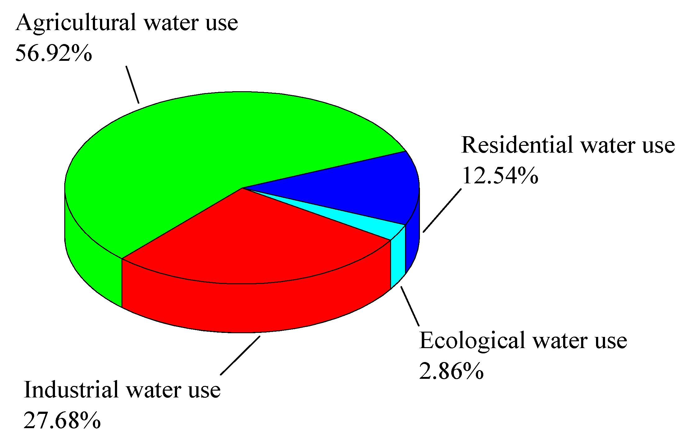
| Total | 491.17 | 135.94 (27.68%) | 279.51 (56.92%) | 61.56 (12.54%) | 14.06 (2.86%) |
| Year | Total Water Use (108 m3) | Industrial Water Use (108 m3) | Agricultural Water Use (108 m3) | Residential Water Use (108 m3) | Ecological Water Use (108 m3) |
|---|---|---|---|---|---|
| 2004 | 26.22 | 8.72 | 14.47 | 2.75 | 0.28 |
| 2005 | 28.14 | 8.30 | 16.92 | 2.60 | 0.32 |
| 2006 | 27.71 | 8.11 | 16.73 | 2.52 | 0.35 |
| 2007 | 32.55 | 7.51 | 21.27 | 2.92 | 0.85 |
| 2008 | 30.42 | 6.90 | 19.73 | 2.94 | 0.85 |
| 2009 | 33.42 | 6.57 | 20.15 | 3.21 | 3.49 |
| 2010 | 30.87 | 7.51 | 17.37 | 3.49 | 2.50 |
| 2011 | 31.26 | 8.97 | 17.70 | 4.03 | 0.56 |
| 2012 | 28.82 | 9.20 | 14.68 | 4.36 | 0.58 |
| 2013 | 32.62 | 9.35 | 18.23 | 4.45 | 0.59 |
| 2014 | 31.42 | 8.92 | 17.35 | 4.54 | 0.61 |
| 2015 | 30.64 | 9.17 | 16.21 | 4.64 | 0.62 |
| 2016 | 31.44 | 9.21 | 16.9 | 4.7 | 0.53 |
| 2017 | 31.54 | 9.28 | 16.84 | 4.78 | 0.64 |
| 2018 | 32.02 | 9.13 | 17.45 | 4.8 | 0.64 |
| 2019 | 32.08 | 9.09 | 17.51 | 4.83 | 0.65 |
| Total | 491.17 | 135.94 (27.68%) | 279.51 (56.92%) | 61.56 (12.54%) | 14.06 (2.86%) |
| Algorithm | Parameter Value | Popsize | Iterations of Number |
|---|---|---|---|
| ESMA | z = 0.03, selected elite proportion pr = 0.1 | 30 | 1000 |
| WOA | value of coefficient vectors : = [2, 0] | 30 | 1000 |
| HHO | E0 randomly changes inside the interval [−1, 1] | 30 | 1000 |
| BBO | The largest immigration rate is 1, largest emigration rate is 1, Mutation rate is 0.1. | 30 | 1000 |
| MVO | Existence probability = [0.2, 1] Exploitation accuracy = 6 | 30 | 1000 |
| AOA | C1 = 2, C2 = 6, C3 = 1, C4 = 2. | 30 | 1000 |
| SMA | z = 0.03 | 30 | 1000 |
| Algorithm | Best MRE | Mean MRE | Worst MRE | Std |
|---|---|---|---|---|
| SSA | 3.7057% | 3.7842% | 4.3348% | 1.3766E-03 |
| WOA | 3.7830% | 9.4189% | 17.6245% | 3.3848E-02 |
| HHO | 3.5682% | 3.8091% | 4.4485% | 2.0942E-03 |
| BBO | 3.6662% | 4.2208% | 6.3299% | 8.0511E-03 |
| MVO | 3.6962% | 3.7246% | 3.7450% | 9.2270E-05 |
| AOA | 3.5694% | 3.9084% | 5.1945% | 4.2159E-03 |
| SMA | 3.7204% | 3.7363% | 3.7643% | 1.3514E-04 |
| ESMA | 3.7084% | 3.7254% | 3.7347% | 5.3146E-05 |
| Algorithm | Best MRE | Mean MRE | Worst MRE | Std |
|---|---|---|---|---|
| SSA | 2.8369% | 2.8381% | 2.8576% | 1.6084E-04 |
| WOA | 2.7940% | 10.6478% | 24.2942% | 6.1449E-02 |
| HHO | 2.8149% | 3.2130% | 4.0381% | 3.5587E-03 |
| BBO | 2.8210% | 2.9604% | 3.4912% | 1.4766E-03 |
| MVO | 2.8132% | 2.8374% | 2.8862% | 1.8078E-04 |
| AOA | 2.8630% | 3.3421% | 4.3456% | 4.5821E-03 |
| SMA | 2.8249% | 2.8394% | 2.8503% | 6.0100E-05 |
| ESMA | 2.8309% | 2.8378% | 2.8489% | 4.9756E-05 |
| Algorithm | Best MRE | Mean MRE | Worst MRE | Std |
|---|---|---|---|---|
| SSA | 2.3868% | 3.1596% | 5.8017% | 7.8594E-03 |
| WOA | 2.9855% | 9.8939% | 17.1511% | 4.5313E-02 |
| HHO | 2.5645% | 2.9217% | 3.3943% | 2.0079E-03 |
| BBO | 2.4364% | 3.0591% | 4.2006% | 4.2337E-03 |
| MVO | 2.4067% | 2.9647% | 3.5502% | 3.1345E-03 |
| AOA | 2.5685% | 3.0042% | 3.6609% | 2.5527E-03 |
| SMA | 2.3783% | 2.6942% | 3.0273% | 1.6634E-03 |
| ESMA | 2.3803% | 2.6488% | 2.8450% | 1.3262E-03 |
| Algorithm | Best MRE | Mean MRE | Worst MRE | Std |
|---|---|---|---|---|
| SSA | 2.8528% | 5.0161% | 9.6486% | 2.1377E-02 |
| WOA | 4.2606% | 16.3721% | 50.7506% | 1.2419E-01 |
| HHO | 2.4567% | 3.5252% | 4.5646% | 6.5378E-03 |
| BBO | 2.4485% | 3.4070% | 5.9116% | 1.0518E-02 |
| MVO | 2.9034% | 5.3989% | 12.8579% | 2.5195E-02 |
| AOA | 2.6473% | 5.7096% | 12.6856% | 3.1945E-02 |
| SMA | 2.4802% | 3.1261% | 4.7669% | 6.7312E-03 |
| ESMA | 2.2954% | 3.1235% | 5.7619% | 8.3033E-03 |
| Year | Population | Gross Industrial Production (108 yuan) | Gross Agricultural Production (108 yuan) |
|---|---|---|---|
| 2020 | 5656114 | 2023.08 | 404.92 |
| 2021 | 5712223 | 2161.82 | 454.77 |
| 2022 | 5768888 | 2310.07 | 510.75 |
| 2023 | 5826116 | 2468.48 | 573.63 |
| 2024 | 5883911 | 2637.76 | 644.25 |
| Algorithm | SSA | WOA | HHO | BBO | MVO | AOA | SMA | ESMA |
|---|---|---|---|---|---|---|---|---|
| Method | Linear Model | |||||||
| 2020 | 37.09 | 42.38 | 35.85 | 38.17 | 36.67 | 33.63 | 36.59 | 36.71 |
| 2021 | 40.68 | 49.25 | 38.50 | 42.26 | 39.97 | 34.77 | 39.88 | 40.05 |
| 2022 | 44.82 | 57.20 | 41.55 | 47.00 | 43.78 | 36.06 | 43.68 | 43.91 |
| 2023 | 49.58 | 66.37 | 45.06 | 52.45 | 48.16 | 37.54 | 48.04 | 48.35 |
| 2024 | 55.05 | 76.93 | 49.08 | 58.73 | 53.19 | 39.22 | 53.04 | 53.44 |
| Method | Logarithmic Model | |||||||
| 2020 | 31.96 | 31.44 | 31.42 | 31.53 | 31.78 | 32.29 | 31.89 | 31.92 |
| 2021 | 32.18 | 31.38 | 31.42 | 31.59 | 31.95 | 32.61 | 32.09 | 32.13 |
| 2022 | 32.41 | 31.33 | 31.43 | 31.65 | 32.12 | 32.93 | 32.29 | 32.35 |
| 2023 | 32.63 | 31.28 | 31.44 | 31.72 | 32.29 | 33.25 | 32.49 | 32.56 |
| 2024 | 32.86 | 31.23 | 31.45 | 31.79 | 32.46 | 33.57 | 32.69 | 32.78 |
| Method | Exponential Model | |||||||
| 2020 | 32.77 | 29.18 | 31.80 | 32.71 | 32.59 | 31.76 | 31.91 | 31.91 |
| 2021 | 33.32 | 24.53 | 31.85 | 33.15 | 33.16 | 31.84 | 32.11 | 32.06 |
| 2022 | 33.77 | 15.13 | 31.86 | 33.64 | 33.65 | 31.92 | 32.26 | 32.16 |
| 2023 | 34.13 | −3.23 | 31.82 | 34.22 | 34.07 | 31.98 | 32.36 | 32.19 |
| 2024 | 34.40 | −38.35 | 31.73 | 34.89 | 34.42 | 32.02 | 32.42 | 32.19 |
| Method | Hybrid Model | |||||||
| 2020 | 33.06 | 28.01 | 32.80 | 31.58 | 33.09 | 33.47 | 32.31 | 30.68 |
| 2021 | 34.07 | 26.86 | 33.34 | 30.35 | 33.26 | 34.59 | 32.31 | 29.39 |
| 2022 | 35.08 | 25.67 | 33.93 | 28.20 | 32.27 | 35.87 | 32.19 | 27.54 |
| 2023 | 36.05 | 24.44 | 34.57 | 24.82 | 29.42 | 37.31 | 31.97 | 25.08 |
| 2024 | 36.96 | 23.14 | 35.29 | 19.82 | 23.64 | 38.95 | 31.63 | 21.95 |
Publisher’s Note: MDPI stays neutral with regard to jurisdictional claims in published maps and institutional affiliations. |
© 2021 by the authors. Licensee MDPI, Basel, Switzerland. This article is an open access article distributed under the terms and conditions of the Creative Commons Attribution (CC BY) license (https://creativecommons.org/licenses/by/4.0/).
Share and Cite
Yu, K.; Liu, L.; Chen, Z. An Improved Slime Mould Algorithm for Demand Estimation of Urban Water Resources. Mathematics 2021, 9, 1316. https://doi.org/10.3390/math9121316
Yu K, Liu L, Chen Z. An Improved Slime Mould Algorithm for Demand Estimation of Urban Water Resources. Mathematics. 2021; 9(12):1316. https://doi.org/10.3390/math9121316
Chicago/Turabian StyleYu, Kanhua, Lili Liu, and Zhe Chen. 2021. "An Improved Slime Mould Algorithm for Demand Estimation of Urban Water Resources" Mathematics 9, no. 12: 1316. https://doi.org/10.3390/math9121316
APA StyleYu, K., Liu, L., & Chen, Z. (2021). An Improved Slime Mould Algorithm for Demand Estimation of Urban Water Resources. Mathematics, 9(12), 1316. https://doi.org/10.3390/math9121316