Article

An Improved Approach of Incomplete Information Fusion and Its Application in Sensor Data-Based Fault Diagnosis

1
School of Computer and Information Science, Southwest University, Chongqing 400715, China
2
School of Big Data and Software Engineering, Chongqing University, Chongqing 401331, China
*
Author to whom correspondence should be addressed.
Mathematics 2021, 9(11), 1292; https://doi.org/10.3390/math9111292
Submission received: 8 May 2021 / Revised: 26 May 2021 / Accepted: 2 June 2021 / Published: 4 June 2021
(This article belongs to the Section Fuzzy Sets, Systems and Decision Making)

Abstract

:
The Dempster–Shafer evidence theory has been widely used in the field of data fusion. However, with further research, incomplete information under the open world assumption has been discovered as a new type of uncertain information. The classical Dempster’s combination rules are difficult to solve the related problems of incomplete information under the open world assumption. At the same time, partial information entropy, such as the Deng entropy is also not applicable to deal with problems under the open world assumption. Therefore, this paper proposes a new method framework to process uncertain information and fuse incomplete data. This method is based on an extension to the Deng entropy in the open world assumption, negation of basic probability assignment (BPA), and the generalized combination rule. The proposed method can solve the problem of incomplete information under the open world assumption, and obtain more uncertain information through the negative processing of BPA, which improves the accuracy of the results. The results of applying this method to fault diagnosis of electronic rotor examples show that, compared with the other uncertain information processing and fusion methods, the proposed method has wider adaptability and higher accuracy, and is more conducive to practical engineering applications.

1. Introduction

Fault diagnosis is an important research content in the engineering industry, and its applications in vehicle detection [1], high-speed train system diagnosis [2,3], and intelligent machinery diagnosis [4] have received a lot of attention. Current research on fault diagnosis mainly includes machine learning and application of diagnostic methods. Some traditional machine learning methods, such as the Gaussian mixture model, support vector machine (SVM), have been widely used in the field of fault diagnosis. A large amount of machinery health information is easier to collect, but it also reduces the efficiency of detection and diagnosis. The data-driven model improves the efficiency of fault diagnosis and is widely used in this field. For example, in the literature [5], a differentiable neural network structure search based on pruning and multi-objective optimization is used for mechanical fault diagnosis, and the multi-scale fuzzy entropy technology based on Euclidean distance is applied to fault diagnosis of industrial system [6].
The above research can effectively improve the efficiency of fault diagnosis, but it is also an important research content for the processing of a large amount of collected information. In complex systems, multi-source information fusion has the advantage of improving accuracy and credibility [7], so it has been widely used. However, affected by the uncertainty of the real world, multi-sensor information sources are considered to be uncertain [8]. For uncertain information, information entropy [9], probability theory [10], rough set theory [11,12], Dempster–Shafer evidence theory [13,14], belief function [15,16], and other methods [17,18] have been proposed to deal with uncertain information. The Dempster–Shafer evidence theory is a type of inexact probability [19], as an uncertain information processing and data fusion tool, it is widely used in pattern recognition [20,21,22], multi-attribute decision-making [23,24], image processing [25] and other fields [26,27,28,29]. Under the Dempster–Shafer evidence theory framework, many uncertain information processing problems can be solved by measuring information uncertainty and using Dempster’s combination rule for fusion, but there are still some open issues that require further research and breakthrough [30,31,32,33].
When studying uncertain information measurement methods, many literatures have followed Klir and Yuan’s classification of information uncertainty: fuzziness and ambiguity [34]. However, with the discovery of research, there is still a new type of uncertain information under the open world assumption, namely incomplete information. This is a type of uncertain information generated by the open world characteristics introduced by the incomplete frame of discernment, new elements, unknown targets, etc. Most of the existing researches focus on the closed world assumption, and it is difficult to solve the problem of incomplete information under the open world assumption.
The re-proposition of the generalized evidence theory [35,36,37] has caused more researchers to pay attention to the studies within the scope of the open world assumption model [38,39,40]. In order to effectively solve the problem of incomplete information processing and fusion under the open world assumption, this paper proposes a new data fusion method, which uses the extension to the Deng entropy in the open world assumption (EDEOW) proposed by Tang et al. [41] to measure the uncertainty of evidence. Combined with the calculation method of the negation of basic probability assignment (BPA) proposed by Yin et al. [42], to obtain the two uncertainties of the original BPA and the negation of BPA of the evidence modeling. The two uncertainties were added as the final uncertainty of the evidence, and the data were modified based on this uncertainty. Such processing considers more uncertainty, which is helpful for improving the accuracy of information processing and reducing information loss. After that, the proposed method uses the generalized combination rule (GCR) [37] under the open world assumption to fuse the modified data. Finally, the method is applied to an example of fault diagnosis to provide decision support for engineers.
The rest of this paper is organized as follows. The preparatory work for the proposed method in this paper are introduced in the second section. The third section proposes a new method based on negation of BPA, EDEOW, and GCR to solve the problem of data fusion in fault diagnosis applications in the open world. The fourth section uses the proposed method to solve a fault diagnosis example. The fifth section applies this method to practical problems in fault diagnosis. The sixth section gives the conclusion of this paper.

2. Preliminaries

In this section, some related information about the Dempster–Shafer evidence theory, Shannon entropy, Deng entropy, and negation of BPA will be briefly introduced.

2.1. Dempster–Shafer Evidence Theory

Some definitions of the Dempster–Shafer Evidence Theory are expressed as follows [13,14]:
Definition 1.
Assuming a non-empty set Ω = { θ 1 ,   θ 2 , ,   θ i , ,   θ N } contains N mutually exclusive events, then such a set Ω is called Frame of Discernment (FOD). A power set of Ω with 2N elements is denoted as:
2 Ω =   { ,   θ 1   ,   θ 2   ,   .   .   .   ,   θ n   ,   θ 1 ,   θ 2   ,   .   .   .   ,   θ 1 ,   θ 2 ,   .   .   .   ,   θ i   ,   .   .   .   ,   Ω } .
Definition 2.
In the frame of discernment, the mass probability function m is a function from the power set 2 to the interval [0,1]. m satisfies the following relation:
m ( ) = 0 , A Ω m A = 1 .
If m(A) > 0, the proposition subset A is called a focal element. m(A) represents the degree of support for proposition A, also known as basic probability assignment (BPA) or basic belief assignment (BBA).
Definition 3.
Body of evidence (BOE) is a binary group composed of a propositional subset and its mass function, and is a unit of uncertain information evidence. BOE is expressed as follows:
( , m ) = { A , m ( A ) : A 2 Ω , m ( A ) > 0 } ,
where, is a subset of the power set 2 Ω .
Definition 4.
The belief function Bel or the plausibility function Pl can be used to express a BPA m:
B e l ( A ) = B A m ( B ) , P l ( A ) = B A m ( B ) ,
where, Bel(A) represents the level of support for the proposition A, and Pl(A) represents the level of no objection to the proposition A.
Definition 5.
Under the framework of the Dempster–Shafer evidence theory, two independent mass functions, m1 and m2, can be fused by the following Dempster’s combination rules:
m ( A ) = ( m 1 m 2 ) ( A ) = 1 1 k B C = A m 1 ( B ) m 2 ( C ) ,
where k is a normalization factor and is defined as follows:
k = B C = m 1 ( B ) m 2 ( C ) .
It should be noted that the classical definition of the Dempster–Shafer evidence theory is defined to be applied in the closed world. For the open world, Deng extended Dempster’s combination rules and named it the generalized combination rule [37].
Definition 6.
In the open world assumption, Deng defined the intersection of two empty sets is still an empty set, satisfying 1 2 = . For the two given BPA m1 and m2, the generalized combination rule is defined as follow:
m ( A ) = ( 1 m ( ) ) B C = A m 1 ( B ) m 2 ( C ) 1 K , K = B C = m 1 ( B ) m 2 ( C ) , m ( ) = m 1 ( ) m 2 ( ) , m ( ) = 1     i f     a n d     o n l y     i f     K = 1 ,
when m(∅) = 0, GCR degenerates to the classic DS combination rule. Two empty sets can be fused by multiplication to obtain their GBPA value. In addition, if and only if K = 1, m(∅) = 1.
With the development of data fusion research under the open world assumption, new literature has proposed the shortcomings of Equation (7). Literature [40] found that the method of obtaining the mass function of the empty set by multiplying the mass function values of two empty sets in the GCR formula is unreasonable, and the result of its combined use with GCR is inconsistent with practice. In addition, because m1(∅) and m2(∅) support each other, and the proposition comes from the open world, the result of their multiplication should not be assigned to the generalized conflict coefficient K, which is inconsistent with the GBPA. Therefore, further studies are needed to improve the GCR. However, since the method proposed in this paper uses the negation of evidence for calculation, it does not involve the multiplication of the mass function values of empty sets, and can effectively avoid the problems proposed in the literature [40].

2.2. Shannon Entropy

The quantitative measurement of information originated from the concept of “information entropy” first proposed by Glaude Shannon in 1948. As an information entropy of uncertainty measurement, the Shannon entropy can effectively solve the uncertainty measurement problem of the probability measurement.
Definition 7.
For N, discrete probability sets p1, p2, ... , pn, the Shannon entropy is defined as follows [43]:
H = p i log p i .

2.3. Belief Entropy

The Deng entropy can be seen as the generalization of the Shannon entropy. It was proposed by Deng in [44], which deals with the belief for each focal element. When BPA degenerates to a probability distribution, the Deng entropy degenerates to the Shannon entropy.
Definition 8.
In FOD X, the Deng entropy is defined as follows:
E d ( m ) = A X m ( A ) log 2 m ( A ) 2 | A | 1 ,
where m is a mass function, |A| is the cardinality of A.
However, when |A| = 0, Equation (9) will not be available. Therefore, Tang et al. [41] extended the uncertainty measure under the Dempster–Shafer evidence theory framework. In the open world assumption, the non-zero mass function of the empty set and the uncertain information represented by the incomplete FOD were handled more carefully.
Definition 9.
Tang et al. defined the extension to Deng’s entropy in the open world (EDEOW) assumption as:
E e d e o w ( m ) = A X m ( A ) log 2 m ( A ) ( 2 ( A + m ( ) X ) 1 ) .
In the formula, |A| is the cardinality of proposition A, |X| is the number of related elements in FOD, and ’⌈⌉’ is the symbol of the ceiling function, which means the smallest integer is not less than the variable, e.g., 0.4 = 1.

2.4. Negation of BPA

The negation method is considered to be a feasible way to express knowledge. Smets defines the negation of the mass function in [45], and used m ¯ to represent the negation of the mass function m in the proposed model. However, this model has some limitations. For example, when applied to the negation of m(θ), m ( θ ¯ ) is always equal to 0. Therefore, Yin et al. proposed a method to calculate negation of the basic probability assignment in [42].
Definition 10.
For each focal element ei in FOD, initial belief assignment pi is replaced by complementary probability 1-pi. After obtaining the negation of m(ei), calculate the sum σ of all focal elements to standardize the belief of all the negative focal elements. Finally, the general formula of the negation of BPA is expressed as:
m ¯ ( e i ) = 1 m ( e i ) n 1 ,
where n is the number of focal elements, and m(ei) is the confidence of the i-th focal element in the initial quality function.

3. An Improved Method for Incomplete Information Fusion in Fault Diagnosis

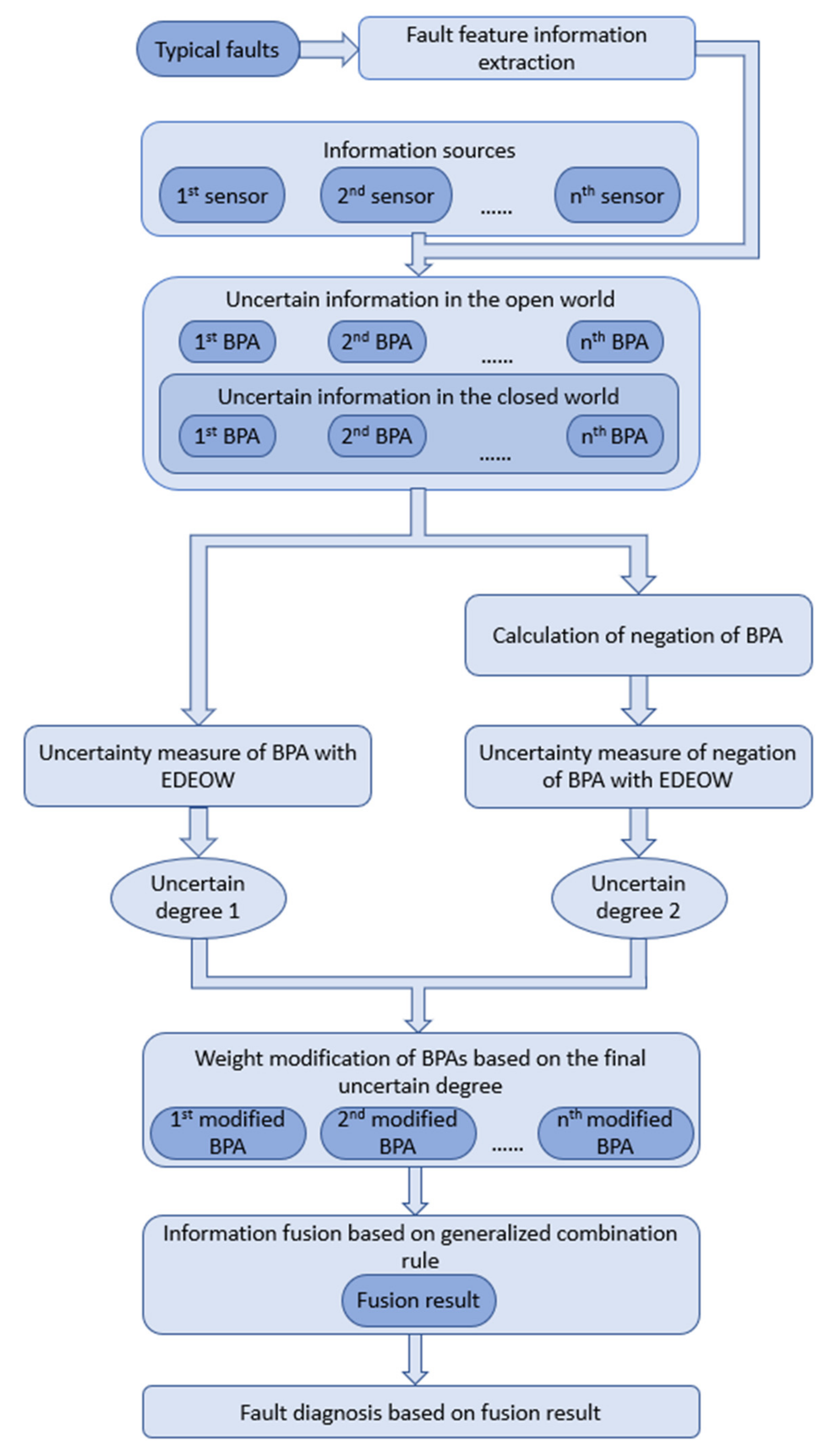
For the problems in the open world, traditional information entropy and DS classical combination rules are difficult to provide solutions. This section proposes a conflict data fusion method based on EDEOW to measure the uncertainty information, obtain more uncertain information through negation of BPA to improve the accuracy of information processing, and adopt GCR for fusion. In Figure 1, a fault diagnosis method framework based on EDEOW, negation of BPA, and GCR in the open world is designed.
The detailed steps of uncertain information processing and fusion are described as follows:
  • Step 1: fault feature extraction and sensor evidence modeling: in multiple fault modes, for each fault feature extracted, evidence modeling is carried out based on the information collected by the sensor. For complete information, the evidence modeling under the open world assumption is the same as that in the closed world. As for incomplete information, the empty set is used to represent it under the open world assumption, and its mass function is non-zero.
  • Step 2: calculation of negation BPA: before data fusion, evidence preprocessing will make the fusion result more accurate. Considering the limitations of data, this paper adopts the method in [42] to calculate the negation of BPA to obtain more uncertain information. For each BOE obtained by modeling, negate it with the following formula:
    m ¯ e i = 1 m e i n 1 .
  • Step 3: uncertainty calculation based on EDEOW: this paper uses the Deng entropy to measure the uncertainty of the data. Since the original Deng entropy is only applicable to the uncertainty measurement in the closed world, this paper adopts the extension to the Deng entropy in the open world assumption [41] proposed by Tang et al., and uses Equation (10) to calculate the uncertainty of BPA and negation of BPA.
  • Step 4: data modification: by summing the two uncertainties of each group of evidence calculated in step 3, the final uncertainty   E e d e o w u m i obtained can be used to calculate the weight of the evidence through the following formula:
    w i = E e d e o w u m i i = 1 m E e d e o w u m i .
Based on the weight of each set of data, the calculation method of modified BPA is calculated in the same way as in the closed world, where mi(A) is the mass function value obtained by proposition A through sensor data modeling:
m w A = i = 1 m w i m i A .
  • Step 5: data fusion based on GCR: considering that the classical Dempster–Shafer theory is not applicable to the problem under the open world assumption, this paper uses the extension rule of Dempster’s combination rule proposed by Deng, namely GCR, to fuse the revised data:
For proposition A in BOE, the result is obtained through (m − 1) times of fusion:
m w 1 A = ( m w m w ) ( A ) = 1 m ( ) 1 k B C = A m w ( B ) m w ( C ) , m w 2 A = ( m w 1 m w ) ( A ) = 1 m ( ) 1 k B C = A m w 1 ( B ) m w ( C ) , …… m w ( m 1 ) A = ( m w ( m 2 ) m w ) ( A ) = 1 m ( ) 1 k B C = A m w ( m 2 ) ( B ) m w ( C ) , m A = ( m w ( m 1 ) m w ) ( A ) = 1 m ( ) 1 k B C = A m w ( m 1 ) ( B ) m w ( C ) .
  • Step 6: application in fault diagnosis: the above information processing and fusion methods are used for fault diagnosis, and the results of the diagnosis will be analyzed and judged based on the fused data.

4. Example

In this section, an example in [46] is used to verify the effectiveness of the method proposed in this paper, and to compare and discuss with other existing methods.

4.1. Example Presentation

Literature [46] extracts the records in the database. Suppose there is a frame of discernment Θ = { F 1 , F 2 , F 3 } , which represents three types of faults that may cause electric shortage in a car: {low oil pressure, air leakage in the intake system, stuck solenoid valve}. Five sensors S1, S2, S3, S4, S5 are placed in different positions to measure the system’s exhaust volume, maximum power, maximum speed and other parameters. Because the engine speed unexpectedly exceeded the upper limit, the sensor S5 was destroyed and could not work normally, resulting in deviations in the measurement results. The purpose of this example is to determine which type of fault occurs in the automotive system through the method proposed in this article.

4.2. Fusion through the Proposed Method

Step 1: after sensors complete the parameter measurement, the central control system models the data obtained by the sensor as BPA, which is shown in Table 1. Where mi corresponds to the evidence modeling result from the sensor Si (I = 1, 2, 3, 4, 5).
It should be noted that the data in literature [46] are in the closed world, while this paper studies the problems under the open world assumption. Considering that the universal set in the closed world represent unknown uncertainty, the m(∅) in the open world also has the same meaning, representing the universal set in the closed world and unknown elements. Therefore, this paper assumes that the BPA assigned to the universal set in the closed world is m(∅), so as to satisfy the open world condition.
Step 2: according to Equation (12), calculate the negation of BPA of the data obtained by the sensor S1 modeling:
m ¯ 1 ( F 1 ) = 1 0.7 4 1 = 0.1 m ¯ 1 ( F 2 ) = 1 0.1 4 1 = 0.3 m ¯ 1 ( F 3 ) = 1 0 4 1 = 0.3333 m ¯ 1 ( ) = 1 0.2 4 1 = 0.2667
The results of the remaining data calculated by the same method are shown in Table 2.
Step 3: use Equation (10) to measure the uncertainty of the original data:
E e d e o w m 1 = 0.7 log 2 0.7 ( 2 ( 1 + 0.2 × 3 ) 1 ) 0.1 log 2 0.1 ( 2 ( 1 + 0.2 × 3 ) 1 ) 0.2 log 2 0.2 ( 2 ( 0 + 0.2 × 3 ) 1 ) = 2.4247 E e d e o w m 2 = 0.7 log 2 0.7 ( 2 ( 1 + 0.3 × 3 ) 1 ) 0.3 log 2 0.3 ( 2 ( 0 + 0.3 × 3 ) 1 ) = 1.9908 E e d e o w m 3 = 0.65 log 2 0.65 ( 2 ( 1 + 0.2 × 3 ) 1 ) 0.15 log 2 0.15 ( 2 ( 1 + 0.2 × 3 ) 1 ) 0.2 log 2 0.2 ( 2 ( 0 + 0.2 × 3 ) 1 ) = 2.5469 E e d e o w m 4 = 0.75 log 2 0.75 ( 2 ( 1 + 0.2 × 3 ) 1 ) 0.05 log 2 0.05 ( 2 ( 1 + 0.2 × 3 ) 1 ) 0.2 log 2 0.2 ( 2 ( 0 + 0.2 × 3 ) 1 ) = 2.2597 E e d e o w m 5 = 0.2 log 2 0.2 ( 2 ( 1 + 0 × 3 ) 1 ) 0.8 log 2 0.8 ( 2 ( 1 + 0 × 3 ) 1 ) = 0.7219
Using the same method, calculate the uncertainty of the negation of BPA obtained in step 2:
E e d e o w m ¯ 1 = 0.1 log 2 0.1 ( 2 ( 1 + 0.2 × 3 ) 1 ) 0.3 log 2 0.3 ( 2 ( 1 + 0.2 × 3 ) 1 ) 0.3333 log 2 0.3333 ( 2 ( 1 + 0.2 × 3 ) 1 ) 0.2667 log 2 0.2667 ( 2 ( 0 + 0.2 × 3 ) 1 ) = 3.0524 E e d e o w m ¯ 2 = 0.1 log 2 0.1 ( 2 ( 1 + 0.2 × 3 ) 1 ) 0.3333 log 2 0.3333 ( 2 ( 1 + 0.2 × 3 ) 1 ) 0.3333 log 2 0.3333 ( 2 ( 1 + 0.2 × 3 ) 1 ) 0.2333 log 2 0.2333 ( 2 ( 0 + 0.2 × 3 ) 1 ) = 3.0937 E e d e o w m ¯ 3 = 0.1167 log 2 0.1167 ( 2 ( 1 + 0.2 × 3 ) 1 ) 0.2833 log 2 0.2833 ( 2 ( 1 + 0.2 × 3 ) 1 ) 0.3333 log 2 0.3333 ( 2 ( 1 + 0.2 × 3 ) 1 ) 0.2667 log 2 0.2667 ( 2 ( 0 + 0.2 × 3 ) 1 ) = 3.0762 E e d e o w m ¯ 4 = 0.0833 log 2 0.0833 ( 2 ( 1 + 0.2 × 3 ) 1 ) 0.3333 log 2 0.3333 ( 2 ( 1 + 0.2 × 3 ) 1 ) 0.3167 log 2 0.3167 ( 2 ( 1 + 0.2 × 3 ) 1 ) 0.2667 log 2 0.2667 ( 2 ( 0 + 0.2 × 3 ) 1 ) = 3.0231 E e d e o w m ¯ 5 = 0.3333 log 2 0.3333 ( 2 ( 1 + 0.2 × 3 ) 1 ) 0.2667 log 2 0.2667 ( 2 ( 1 + 0.2 × 3 ) 1 ) 0.0667 log 2 0.0667 ( 2 ( 1 + 0.2 × 3 ) 1 ) 0.3333 log 2 0.3333 ( 2 ( 0 + 0.2 × 3 ) 1 ) = 2.8824
Step 4: add the two uncertainties obtained in step 3 to calculate the   E e d e o w u m i (I = 1, 2, 3, 4, 5) of each group of evidence:
E e d e o w u m 1 =   2.4247 + 3.0524 = 5.4771 E e d e o w u m 2 =   1.9908 + 3.0937 = 5.0845 E e d e o w u m 3 =   2.5469 + 3.0762 = 5.6231 E e d e o w u m 4 =   2.2597 + 3.0231 = 5.2828 E e d e o w u m 5 =   0.7219 + 2.8824 = 3.6043
Using Equation (13), calculate the weight of each group of evidence:
w 1 = 5.4771 5.4771 + 5.0845 + 5.6231 + 5.2828 + 3.6043 = 0.2185 w 2 = 5.0845 5.4771 + 5.0845 + 5.6231 + 5.2828 + 3.6043 = 0.2028 w 3 = 5.6231 5.4771 + 5.0845 + 5.6231 + 5.2828 + 3.6043 = 0.2243 w 4 = 5.2828 5.4771 + 5.0845 + 5.6231 + 5.2828 + 3.6043 = 0.2107 w 5 = 3.6043 5.4771 + 5.0845 + 5.6231 + 5.2828 + 3.6043 = 0.1438
Based on the calculated weights and according to Equation (14), the BPA is modified as follows:
m w F 1 = 0.7 × 0.2185 + 0.7 × 0.2028 + 0.65 × 0.2243 + 0.75 × 0.2107 + 0 × 0.1438 = 0.5987 m w F 2 = 0.1 × 0.2185 + 0 × 0.2028 + 0.15 × 0.2243 + 0 × 0.2107 + 0.2 × 0.1438 = 0.0843 m w F 3 = 0 × 0.2185 + 0 × 0.2028 + 0 × 0.2243 + 0.05 × 0.2107 + 0.8 × 0.1438 = 0.1256 m w ( ) = 0.2 × 0.2185 + 0.3 × 0.2028 + 0.2 × 0.2243 + 0.2 × 0.2107 + 0 × 0.1438 = 0.1914
Step 5: use Equation (15) to fuse the modified BPA:
m F 1 = ( ( ( ( m w m w ) 1 m w ) 2 m w ) 3 m w ) 4 ( F 1 ) = 0.9993 m F 2 = ( ( ( ( m w m w ) 1 m w ) 2 m w ) 3 m w ) 4 ( F 2 ) = 0.0001 m F 3 = ( ( ( ( m w m w ) 1 m w ) 2 m w ) 3 m w ) 4 ( F 3 ) = 0.0004 m = ( ( ( ( m w m w ) 1 m w ) 2 m w ) 3 m w ) 4 ( ) = 0.0003

4.3. Analysis

Since the universal set in the closed world has the same meaning as m(∅) under the open world assumption, the BPA value assigned to the universal set in the research in the closed world is assumed to be m(∅) to satisfy the open world condition. Table 3 and Figure 2 show the fusion results of the method proposed in this paper and other existing methods for this problem. Based on the threshold ∆ = 0.70 set by the literature [47], if m(Fi) ≥ 0.70 exists in the fusion result, it means that the method has successfully identified the fault type Fi.
In this example, because the sensor S5 was destroyed, the data collected from S5 conflicted with other evidence after modeling, and most of the beliefs were mistakenly assigned to F3. With this in mind, combined with the results in Table 3, it can be concluded that F1 is the fault that caused the shortage of power in the automotive system.
As shown in Table 3, the classic DS combination rules are affected when dealing with conflicting data, and most of the beliefs are incorrectly assigned to F3, which fails to solve the problem in this example. Sun et al.’s method did not reach the set threshold ∆ = 0.7, and the type of failure could not be diagnosed. Deng et al., Wang et al., and the method proposed in this paper all overcome the impact of conflicting data and successfully identify the fault type as F1. Compared with the complex matrix operation in the method proposed by Deng et al., the proposed method has lower computational complexity and higher reliability. Meanwhile, compared with the fusion method proposed by Wang et al., the method proposed in this paper introduces the concept of negation of BPA. By obtaining more uncertain information in the process of data preprocessing, the accuracy of fusion results is improved and the fault types can be diagnosed more accurately.

5. Application

In order to further test the effectiveness and applicability of the method proposed in this paper in solving the problem of fault diagnosis based on sensor data, the case in literature [50] is used as an example for diagnosis and verification in this section.

5.1. Problem Description

Suppose the motor rotor has three different types of faults, which are F = {rotor unbalance, rotor misalignment, pedestal loosening}. Three acceleration sensors installed at different positions are used to measure the vibration acceleration of the motor rotor. The amplitude of acceleration vibration frequency at different frequencies is defined as a fault feature variable.
In reference [50], the sensor’s support and credibility were calculated through the similarity matrix of the characteristic variables. After determining the Z-number, the membership function corresponding to component A was matched with typical faults to obtain BPA. The BPAs obtained by modeling the data collected by the sensors are shown in Table 4.

5.2. Implementation Steps

Step 1: in this example, three different frequencies, Freq1, Freq2, and Freq3, are used as fault feature variables to implement fault diagnosis. Since the main research content of this case is to use an improved incomplete information fusion method for fault diagnosis based on sensor data, the method of data modeling as BPA is not the main content of this paper. Therefore, this section directly adopts the BPA data reported by sensors in the literature [50], which is shown in Table 4.
Step 2: according to the description in the third section, this paper adopts Equation (12) proposed by Yin et al. to negate BPA. The negation of BPA at Freq1 vibration acceleration frequency is calculated as follows:
m ¯ s 1 { F 2 } = 1 0.8176 4 1 = 0.0608 m ¯ s 1 { F 3 } = 1 0.0003 4 1 = 0.3332 m ¯ s 1 { F 1 , F 2 } = 1 0.1553 4 1 = 0.2816 m ¯ s 1 = 1 0.0268 4 1 = 0.3244 m ¯ s 2 { F 2 } = 1 0.5658 4 1 = 0.1447 m ¯ s 2 { F 3 } = 1 0.0009 4 1 = 0.3330 m ¯ s 2 { F 1 , F 2 } = 1 0.0646 4 1 = 0.3118 m ¯ s 2 = 1 0.3687 4 1 = 0.2104 m ¯ s 3 { F 2 } = 1 0.2403 4 1 = 0.2532 m ¯ s 3 { F 3 } = 1 0.0004 4 1 = 0.3332 m ¯ s 3 { F 1 , F 2 } = 1 0.0141 4 1 = 0.3286 m ¯ s 3 = 1 0.7452 4 1 = 0.0849
According to Equation (12), the data calculation results of Freq2 and Freq3 are shown in Table 5.
Step 3: on the basis of the previous step, we use the EDEOW, which proposed by Tang et al. under the open world assumption, to further preprocess the uncertain information. Through Equation (10), the uncertainty of each BOE at the frequency of Freq1 is measured as follows:
E e d e o w ( m s 1 ) = 0.8176 log 2 0.8176 ( 2 ( 1 + 0.0268 × 3 ) 1 ) 0.0003 log 2 0.0003 ( 2 ( 1 + 0.0268 × 3 ) 1 ) 0.1553 log 2 0.1553 ( 2 ( 2 + 0.0268 × 3 ) 1 ) 0.0268 log 2 0.0268 ( 2 ( 0 + 0.0268 × 3 ) 1 ) = 2.5306 E e d e o w ( m s 2 ) = 0.5658 log 2 0.5658 ( 2 ( 1 + 0.3687 × 3 ) 1 ) 0.0009 log 2 0.0009 ( 2 ( 1 + 0.3687 × 3 ) 1 ) 0.0646 log 2 0.0646 ( 2 ( 2 + 0.3687 × 3 ) 1 ) 0.3687 log 2 0.3687 ( 2 ( 0 + 0.3687 × 3 ) 1 ) = 3.6877 E e d e o w ( m s 2 ) = 0.2403 log 2 0.2403 ( 2 ( 1 + 0.7452 × 3 ) 1 ) 0.0004 log 2 0.0004 ( 2 ( 1 + 0.7452 × 3 ) 1 ) 0.0141 log 2 0.0141 ( 2 ( 2 + 0.7452 × 3 ) 1 ) 0.7452 log 2 0.7452 ( 2 ( 0 + 0.7452 × 3 ) 1 ) = 4.0040
The uncertainty measurement results at Freq2 and Freq3 frequencies are shown in Table 6.
In addition, it is also necessary to measure uncertainty of the negation of BPA. Through the same formula, the uncertainty calculation results of the negation of BPA at Freq1, Freq2 and Freq3 are shown in Table 7.
Step 4: by adding the two uncertainties calculated in the third step, the calculation process of the final uncertainty of each group of evidence at Freq1 is as follows:
  E e d e o w u m s 1 = 2.5306 + 3.2307 = 5.7613 E e d e o w u m s 2 =   3.6877 + 3.5617 = 7.2494 E e d e o w u m s 3 =   4.0040 + 3.7117 = 7.7157
The final uncertain degree of each group of evidence is shown in Table 8.
The final uncertainty is used to modify the data. According to Equation (13), the weight of each data under Freq1 vibration acceleration frequency is calculated as follows:
w s 1 = 5.7613 5.7613 + 7.2494 + 7.7157 = 0.2780 w s 2 = 7.2494 5.7613 + 7.2494 + 7.7157 = 0.3498 w s 3 = 7.7157 5.7613 + 7.2494 + 7.7157 = 0.3723
The weight calculation results at Freq2 and Freq3 frequencies are shown in Table 9.
After calculating the weight of each group of data, according to Equation (14), calculate the modified BPA under Freq1:
m w { F 2 } = 0.8176 × 0.2780 + 0.5658 × 0.3498 + 0.2403 × 0.3723 = 0.5147 m w { F 3 } = 0.0003 × 0.2780 + 0.0009 × 0.3498 + 0.0004 × 0.3723 = 0.0005 m w { F 1 , F 2 } = 0.1553 × 0.2780 + 0.0646 × 0.3498 + 0.0141 × 0.3723 = 0.0710 m w ( ) = 0.0268 × 0.2780 + 0.3687 × 0.3498 + 0.7452 × 0.3723 = 0.4139
The modification results of BPA at other frequencies are shown in Table 10.
Step 5: after the modification of BPAs, based on the GCR shown in Equation (15), two fusion operations are required for each data at the Freq1 frequency. The calculation process is as follows:
m { F 2 } = ( m w m w 1 m w ) 2 { F 2 } = 0.9286 m { F 3 } = ( m w m w 1 m w ) 2 { F 3 } = 0.0000 m { F 1 , F 2 } = ( m w m w 1 m w ) 2 { F 1 , F 2 } = 0.0017 m = ( m w m w 1 m w ) 2 = 0.0709
Finally, the fusion results at all frequencies are calculated in the same way and shown in Table 11.

5.3. Discussion

Table 12 shows the data fusion results of different methods in fault diagnosis applications.
The fusion results of different methods are compared intuitively in Figure 3.
As shown in Table 11, among all test frequencies, F2 has the highest confidence support degree among all test frequencies, which indicates that the fault diagnosis result is F2. According to Table 12 and Figure 3, the diagnosis results of the proposed method are consistent with those obtained by other literature methods, which verifies the effectiveness of this method. In addition, compared with the method in the literature [41,50], the method proposed in this paper has a higher confidence for the identified fault type F2, which is more conducive to the decision-making of relevant personnel in practical engineering applications.
The incomplete information fusion method proposed in this paper has a good effect on the problem of this application. In addition, for the example in Section 4, this method can be used to diagnose effectively and with high accuracy. Therefore, the proposed method is applicable for fault diagnosis based on any sensor data. With the proposed method, we assume that there is unknown fault type. This idea gives space for unknown fault type by assigning a belief on the empty set which represents other potential fault type. More importantly, the proposed idea has no bad effect on identifying the available fault condition.

6. Conclusions

In order to solve the problem of incomplete information under the open world assumption, this paper proposes an incomplete information processing method based on negation of BPA, EDEOW, and GCR. In this paper, the negation of the BPA calculation method proposed by Yin et al. is adopted to obtain more uncertain information, thus reducing information loss and improving information processing accuracy. An extension to the Deng entropy in the open world assumption is an extended uncertainty measurement method based on belief structure. The method proposed in this paper uses EDEOW to measure the uncertainty of original BPA and negation of BPA. The two groups of measured uncertainties are added together as the final uncertainty. Based on this uncertainty, the weight of evidence is calculated and the data are modified, and the modification results are more accurate. The generalized combination rule is an extension of the Dempster–Shafer theory in the open world. It solves the problem that the classical combination rule of the Dempster–Shafer evidence theory cannot be applied to the open world assumption. It is used for the final fusion of the modified data in the proposed method. Compared with other methods, the new information processing strategy constructed in this paper considers more uncertainties and makes the measurement results more accurate. At the same time, the EDEOW and GCR used in this method are both applicable for the problems under the open world assumption, effectively making up for the shortcomings of traditional methods that are difficult to solve the problem of incomplete information. Finally, this method is applied to the problem of fault diagnosis, which is more conducive to the decision-making of engineers in practical applications.

Author Contributions

Conceptualization, Y.C. and Y.T.; methodology, Y.C. and Y.T.; writing—original draft preparation, Y.C.; writing—review and editing, Y.T. All authors have read and agreed to the published version of the manuscript.

Funding

This research was partially supported by the National Key Research and Development Project of China (grant no. 2020YFB1711900).

Institutional Review Board Statement

Not applicable.

Informed Consent Statement

Not applicable.

Data Availability Statement

All relevant data are within the paper.

Conflicts of Interest

The authors declare no conflict of interest.

References

  1. Shi, Q.; Zhang, H. Fault diagnosis of an autonomous vehicle with an improved SVM algorithm subject to unbalanced datasets. IEEE Trans. Ind. Electron. 2020, 68, 6248–6256. [Google Scholar] [CrossRef]
  2. Cheng, C.; Wang, W.; Chen, H.; Zhang, B.; Shao, J.; Teng, W. Enhanced Fault Diagnosis Using Broad Learning for Traction Systems in High-Speed Trains. IEEE Trans. Power Electron. 2020, 36, 7461–7469. [Google Scholar] [CrossRef]
  3. Zhang, K.; Jiang, B.; Chen, F. Multiple-Model Based Diagnosis of Multiple Faults with High Speed Train Applications Using Second Level Adaptation. IEEE Trans. Ind. Electron. 2020, 68, 6257–6266. [Google Scholar] [CrossRef]
  4. Li, X.; Zhang, W. Deep learning-based partial domain adaptation method on intelligent machinery fault diagnostics. IEEE Trans. Ind. Electron. 2020, 68, 4351–4361. [Google Scholar] [CrossRef]
  5. Zhang, K.; Chen, J.; He, S.; Xu, E.; Li, F.; Zhou, Z. Differentiable neural architecture search augmented with pruning and multi-objective optimization for time-efficient intelligent fault diagnosis of machinery. Mech. Syst. Signal Process. 2021, 158, 107773. [Google Scholar] [CrossRef]
  6. Zhou, R.; Wang, X.; Wan, J.; Xiong, N. EDM-Fuzzy: An Euclidean Distance Based Multiscale Fuzzy Entropy Technology for Diagnosing Faults of Industrial Systems. IEEE Trans. Ind. Inform. 2020, 17, 4046–4054. [Google Scholar] [CrossRef]
  7. Wu, D.; Liu, Z.; Tang, Y. A new classification method based on the negation of a basic probability assignment in the evidence theory. Eng. Appl. Artif. Intell. 2020, 96, 103985. [Google Scholar] [CrossRef]
  8. Meng, X.L.; Gong, L.T.; Yao, J.C. A fuzzy evaluation approach with the quasi-ordered set: Evaluating the efficiency of decision making units. Fuzzy Optim. Decis. Mak. 2020, 19, 297–310. [Google Scholar] [CrossRef]
  9. Shannon, C.E. A mathematical theory of communication. ACM SIGMOBILE Mob. Comput. Commun. Rev. 2021, 5, 3–55. [Google Scholar] [CrossRef]
  10. Dubois, D.; Prade, H. Possibility theory, probability theory and multiple-valued logics: A clarification. Ann. Math. Artif. Intell. 2001, 32, 35–66. [Google Scholar] [CrossRef]
  11. Pawlak, Z. Rough sets. Int. J. Comput. Inf. Sci. 1982, 11, 341–356. [Google Scholar] [CrossRef]
  12. Walczak, B.; Massart, D.L. Rough sets theory. Chemom. Intell. Lab. Syst. 1999, 47, 1–16. [Google Scholar] [CrossRef]
  13. Dempster, A.P. Upper and lower probabilities induced by a multivalued mapping. In Classic Works of the Dempster-Shafer Theory of Belief Functions; Springer: Berlin/Heidelberg, Germany, 2008; pp. 57–72. [Google Scholar]
  14. Shafer, G. A Mathematical Theory of Evidence; Princeton University Press: Princeton, NJ, USA, 1976; Volume 42. [Google Scholar]
  15. Liu, Z.G.; Pan, Q.; Dezert, J.; Mercier, G. Hybrid classification system for uncertain data. IEEE Trans. Syst. ManCybern. Syst. 2016, 47, 2783–2790. [Google Scholar] [CrossRef] [Green Version]
  16. Zhou, K.; Martin, A.; Pan, Q.; Liu, Z. SELP: Semi-supervised evidential label propagation algorithm for graph data clustering. Int. J. Approx. Reason. 2018, 92, 139–154. [Google Scholar] [CrossRef] [Green Version]
  17. Ding, J.; Han, D.; Dezert, J.; Yang, Y. A new hierarchical ranking aggregation method. Inf. Sci. 2018, 453, 168–185. [Google Scholar] [CrossRef] [Green Version]
  18. Tang, Y.; Wu, D.; Liu, Z. A new approach for generation of generalized basic probability assignment in the evidence theory. Pattern Anal. Appl. 2021, 1–17. [Google Scholar] [CrossRef]
  19. Walley, P. Towards a unified theory of imprecise probability. Int. J. Approx. Reason. 2000, 24, 125–148. [Google Scholar] [CrossRef] [Green Version]
  20. Zhou, K.; Martin, A.; Pan, Q.; Liu, Z.G. Median evidential c-means algorithm and its application to community detection. Knowl. Based Syst. 2015, 74, 69–88. [Google Scholar] [CrossRef] [Green Version]
  21. Liu, Z.G.; Liu, Y.; Dezert, J.; Cuzzolin, F. Evidence combination based on credal belief redistribution for pattern classification. IEEE Trans. Fuzzy Syst. 2019, 28, 618–631. [Google Scholar] [CrossRef] [Green Version]
  22. Jing, M.; Tang, Y. A new base basic probability assignment approach for conflict data fusion in the evidence theory. Appl. Intell. 2021, 51, 1056–1068. [Google Scholar] [CrossRef]
  23. Fu, C.; Yang, S. An evidential reasoning based consensus model for multiple attribute group decision analysis problems with interval-valued group consensus requirements. Eur. J. Oper. Res. 2012, 223, 167–176. [Google Scholar] [CrossRef]
  24. Fu, C.; Chang, W.; Yang, S. Multiple criteria group decision making based on group satisfaction. Inf. Sci. 2020, 518, 309–329. [Google Scholar] [CrossRef]
  25. Zhu, Y.M.; Bentabet, L.; Dupuis, O.; Kaftandjian, V.; Babot, D.; Rombaut, M. Automatic determination of mass functions in Dempster-Shafer theory using fuzzy c-means and spatial neighborhood information for image segmentation. Opt. Eng. 2002, 41, 760–770. [Google Scholar] [CrossRef]
  26. Fu, C.; Chin, K.S. Robust evidential reasoning approach with unknown attribute weights. Knowl. Based Syst. 2014, 59, 9–20. [Google Scholar] [CrossRef]
  27. Su, X.; Mahadevan, S.; Xu, P.; Deng, Y. Dependence assessment in human reliability analysis using evidence theory and AHP. Risk Anal. 2015, 35, 1296–1316. [Google Scholar] [CrossRef]
  28. Hatefi, S.M.; Basiri, M.E.; Tamošaitienė, J. An evidential model for environmental risk assessment in projects using Dempster–Shafer theory of evidence. Sustainability 2019, 11, 6329. [Google Scholar] [CrossRef] [Green Version]
  29. Wu, D.; Tang, Y. An improved failure mode and effects analysis method based on uncertainty measure in the evidence theory. Qual. Reliab. Eng. Int. 2020, 36, 1786–1807. [Google Scholar] [CrossRef]
  30. Murphy, C.K. Combining belief functions when evidence conflicts. Decis. Support Syst. 2000, 29, 1–9. [Google Scholar] [CrossRef]
  31. Schubert, J. Conflict management in Dempster–Shafer theory using the degree of falsity. Int. J. Approx. Reason. 2011, 52, 449–460. [Google Scholar] [CrossRef] [Green Version]
  32. Deng, X.; Jiang, W. On the negation of a Dempster–Shafer belief structure based on maximum uncertainty allocation. Inf. Sci. 2020, 516, 346–352. [Google Scholar] [CrossRef] [Green Version]
  33. Jiroušek, R.; Shenoy, P.P. On properties of a new decomposable entropy of Dempster-Shafer belief functions. Int. J. Approx. Reason. 2020, 119, 260–279. [Google Scholar] [CrossRef]
  34. Klir, G.; Yuan, B. Fuzzy Sets and Fuzzy Logic; Prentice Hall: Hoboken, NJ, USA, 1995; Volume 4. [Google Scholar]
  35. Deng, Y.; Jiang, W.; Han, D. Basic frame of generalized evidence theory. J. Xi’an Jiaotong Univ. 2010, 44, 119–124. [Google Scholar]
  36. Deng, Y.; Han, D. Methods to determine generalized basic probability assignment in generalized evidence theory. J. Xi’an Jiaotong Univ. 2011, 45, 34–38. [Google Scholar]
  37. Deng, Y. Generalized evidence theory. Appl. Intell. 2015, 43, 530–543. [Google Scholar] [CrossRef] [Green Version]
  38. Jiang, W.; Zhan, J.; Zhou, D.; Li, X. A method to determine generalized basic probability assignment in the open world. Math. Probl. Eng. 2016, 2016. [Google Scholar] [CrossRef]
  39. Daniel, M. A relationship of conflicting belief masses to open world assumption. In International Conference on Belief Functions; Springer: Cham, Germany, 2016; pp. 146–155. [Google Scholar]
  40. Jiang, W.; Zhan, J. A modified combination rule in generalized evidence theory. Appl. Intell. 2017, 46, 630–640. [Google Scholar] [CrossRef]
  41. Tang, Y.; Zhou, D.; Chan, F.T. An extension to Deng’s entropy in the open world assumption with an application in sensor data fusion. Sensors 2018, 18, 1902. [Google Scholar] [CrossRef] [PubMed] [Green Version]
  42. Yin, L.; Deng, X.; Deng, Y. The negation of a basic probability assignment. IEEE Trans. Fuzzy Syst. 2018, 27, 135–143. [Google Scholar] [CrossRef]
  43. Shannon, C.E. A mathematical theory of communication. Bell Syst. Tech. J. 1948, 27, 379–423. [Google Scholar] [CrossRef] [Green Version]
  44. Deng, Y. Deng entropy. Chaos Solitons Fractals 2016, 91, 549–553. [Google Scholar] [CrossRef]
  45. Smets, P. The application of the matrix calculus to belief functions. Int. J. Approx. Reason. 2002, 31, 1–30. [Google Scholar] [CrossRef] [Green Version]
  46. Wang, Z.; Xiao, F. An improved multi-source data fusion method based on the belief entropy and divergence measure. Entropy 2019, 21, 611. [Google Scholar] [CrossRef] [Green Version]
  47. Jiang, W.; Wei, B.; Xie, C.; Zhou, D. An evidential sensor fusion method in fault diagnosis. Adv. Mech. Eng. 2016, 8. [Google Scholar] [CrossRef] [Green Version]
  48. Sun, Q.; Ye, X.Q.; Gu, W.K. A new combination rules of evidence theory. Acta Electron. Sin. 2000, 28, 117–119. [Google Scholar]
  49. Yong, D.; Wenkang, S.; Zhenfu, Z.; Qi, L. Combining belief functions based on distance of evidence. Decis. Support Syst. 2004, 38, 489–493. [Google Scholar] [CrossRef]
  50. Jiang, W.; Xie, C.; Zhuang, M.; Shou, Y.; Tang, Y. Sensor data fusion with z-numbers and its application in fault diagnosis. Sensors 2016, 16, 1509. [Google Scholar] [CrossRef] [PubMed]
Figure 1. The proposed data fusion method based on EDEOW, negation of BPA, and GCR.
Mathematics 09 01292 g001
Figure 2. Fusion results of different methods in example.
Mathematics 09 01292 g002
Figure 3. Data fusion results of different methods in fault diagnosis.
Mathematics 09 01292 g003
Table 1. Sensor data modeled as BPAs.
F1F2F3
m10.700.1000.20
m20.70000.30
m30.650.1500.20
m40.7500.050.20
m500.200.800
Table 2. Negation of BPAs of example.
F1F2F3
m ¯ 1 0.100.300.33330.2667
m ¯ 2 0.100.33330.33330.2333
m ¯ 3 0.11670.28330.33330.2667
m ¯ 4 0.08330.33330.31670.2667
m ¯ 5 0.33330.26670.06670.3333
Table 3. Fusion results of example.
F1F2F3
DS [13]0.00000.34430.65570.0000
Sun et al. [48]0.40280.06600.12470.4028
Deng et al. [49]0.99330.00300.00280.0008
Wang et al. [46]0.99340.00330.00250.0008
The proposed method0.99930.00010.00040.0003
Table 4. Fault diagnosis data modeled as BPAs.
Freq1Freq2Freq3
{F2}{F3}{F1, F2}{F2}{F1}{F2}{F1, F2}
ms1(·)0.81760.00030.15530.02680.62290.37710.36660.45630.11850.0586
ms2(·)0.56580.00090.06460.36870.76600.23410.27930.41510.26520.0404
ms3(·)0.24030.00040.01410.74520.85980.14020.28970.43310.24700.0302
Table 5. Negation of BPAs.
Negation of BPAsFreq1Freq2Freq3
{F2}{F3}{F1, F2}{F2}{F1}{F2}{F1, F2}
m ¯ s 1 · 0.06080.33320.28160.32440.37710.62290.21110.18120.29380.3138
m ¯ s 2 · 0.14470.33300.31180.21040.23410.76590.24020.19500.24490.3199
m ¯ s 3 · 0.25320.33320.32860.08490.14020.85980.23670.18900.25110.3232
Table 6. Uncertainty measurement results of BPAs based on EDEOW.
Eedeow(·)Freq1Freq2Freq3
E e d e o w m s 1 2.53063.30243.2887
E e d e o w m s 2 3.68771.99913.5804
E e d e o w m s 3 4.00401.94753.5305
Table 7. Uncertainty measurement results of negation of BPAs based on EDEOW.
Eedeow(·)Freq1Freq2Freq3
E e d e o w m ¯ s i 3.23073.00193.4107
E e d e o w m ¯ s 2 3.56173.84983.3545
E e d e o w m ¯ s 3 3.71173.54483.3532
Table 8. Uncertain degree of BPAs.
Eedeowu(·)Freq1Freq2Freq3
E e d e o w u m ¯ s i 5.76136.30436.6994
E e d e o w u m ¯ s 2 7.24945.84896.9349
E e d e o w u m ¯ s 3 7.71575.49236.8837
Table 9. Weight of BOEs.
W s i ( ) Freq1Freq2Freq3
W s 1 ( ) 0.27800.35730.3265
W s 2 ( ) 0.34980.33150.3380
W s 3 ( ) 0.37230.31130.3355
Table 10. Modification BPAs based on the proposed method.
Modification BPAsFreq1Freq2Freq3
{F2}{F3}{F1, F2}{F2}{F1}{F2}{F1, F2}
m w · 0.51470.00050.07100.41390.74410.25600.31130.43460.21120.0429
Table 11. Data fusion results for fault diagnosis.
Freq1Freq2Freq3
{F2}{F3}{F1, F2}{F2}{F1}{F2}{F1, F2}
Results0.92860.00000.00170.07090.98380.01680.33090.64560.02340.0001
Table 12. Data fusion results of different methods in fault diagnosis.
Freq1Freq2Freq3
{F2}{F3}{F1, F2}{F2}{F1}{F2}{F1, F2}
Jiang et al.’s method [50]0.88610.00020.0582-0.9621-0.33840.59040.0651-
Tang et al.’s method [41]0.91810.00000.00150.08030.97960.02060.33030.64590.02380.0001
The proposed method0.92860.00000.00170.07090.98380.01680.33090.64560.02340.0001
Publisher’s Note: MDPI stays neutral with regard to jurisdictional claims in published maps and institutional affiliations.

