Abstract
This paper presents a new framework based on geometric algebra (GA) to solve and analyse three-phase balanced electrical circuits under sinusoidal and non-sinusoidal conditions. The proposed approach is an exploratory application of the geometric algebra power theory (GAPoT) to multiple-phase systems. A definition of geometric apparent power for three-phase systems, that complies with the energy conservation principle, is also introduced. Power calculations are performed in a multi-dimensional Euclidean space where cross effects between voltage and current harmonics are taken into consideration. By using the proposed framework, the current can be easily geometrically decomposed into active- and non-active components for current compensation purposes. The paper includes detailed examples in which electrical circuits are solved and the results are analysed. This work is a first step towards a more advanced polyphase proposal that can be applied to systems under real operation conditions, where unbalance and asymmetry is considered.
1. Introduction
For more than a century, the steady-state operation of AC electrical circuits has been analysed in the frequency domain using complex numbers. The foundations of this well-established technique were initially developed by Steinmetz [1] and later refined by other authors such as Kennelly [2] or Heaviside [3]. In its basic form, an AC signal is transformed from the time to the frequency domain, where algebraic equations can be easily manipulated. This transformation is commonly referred to as phasor transformation. For example, the phasor representation of a voltage waveform such as is
while the inverse transformation is given by
This methodology is widely applied to solve single- and three-phase electrical circuits that operate in steady state under sinusoidal conditions.
It can also be applied to circuits operating under non-sinusoidal conditions by using the superposition theorem. In this case, the voltage and current components of each harmonic frequency are calculated separately, one by one, and then added in the time domain so that the voltage and current waveforms are obtained. Nevertheless, this property can be seen as both an advantage and a disadvantage. The main reason is that bilinear operations, such as products between voltages and currents of different frequencies, are not meaningful in the algebra of complex numbers when applied to power systems. However, this procedure is strictly required to calculate power flows under distorted conditions. For example, consider a voltage and a current . Their phasor representations are and , respectively. Even though these signals are completely different, their representation in the complex domain is the same. From a mathematical perspective, the product cannot be performed since only rotating vectors of the same frequency (and, thus, phasor quantities) can be axiomatically multiplied in the complex domain. Due to the aforementioned limitations, the principle of energy (power) conservation cannot be applied to apparent power in the complex domain in a general sense [4]. These drawbacks have given rise to a great number of proposals for the resolution of electrical circuits and the analysis of power flows [5,6,7]. This topic is of a paramount relevance because of the increasing energy losses in transmission systems as well as the negative effects on electrical-drives, power transformers and electronic devices.
Recently, geometric algebra (GA) has been proposed and applied to solve physical and engineering problems [8,9]. It has also been proposed for analysing electrical circuits [10,11]. The use of GA has shed some light on a number of important shortcomings of complex numbers, mainly due to the following properties:
- It is possible to perform calculations between voltages and currents of different frequencies that generate cross-coupling power terms. Therefore, power under non-sinusoidal conditions can be adequately calculated;
- Foundations of GA circuit analysis is defined in a multi-dimensional geometric domain , where a definition of geometric apparent power that fulfils the principle of energy conservation can be obtained [12]. This power has been named geometric apparent power in the literature. Compared to the traditional definition of apparent power , it considers the contribution of cross effects between voltages and currents of different frequencies and is a signed quantity.
The aforementioned statements are strongly supported by the very basic foundations of electromagnetic power theory: the Poynting Theorem. It is well-known that the density power delivered to a load can be calculated through the Poynting vector
where and are the electric and magnetic field vector, respectively. Note the cross product in (3). If both the electric field and the magnetic field are transferred to the frequency domain [13], it is evident that the product of the harmonics content of different frequencies leads to a density power with a clear physical existence.
The concept of geometric apparent power was first introduced by Menti in 2007 [14]. It was demonstrated that the traditional apparent power is a particular case of the geometric apparent power for systems that operate under sinusoidal conditions. Later, in 2010, Castro-Núñez presented a new mathematical framework based on the use of k-blades in GA for solving and analysing electrical circuits under sinusoidal conditions [15]. The concept of geometric impedance was introduced and applied to single-phase RLC circuits. The theory was extended by the same author for non-linear circuits in the presence of harmonics [16,17]. The improvements compared to traditional theories were demonstrated through examples. However, some drawbacks and inconveniences were found in this particular formulation [18]. Castilla and Bravo [19,20] made improvements to former theories and presented an alternative formulation, called generalized complex geometric algebra. This theory can be used to perform power calculations, but cannot solve electrical circuits in the GA domain. Recently, Montoya et al. [10,11] have studied power flows under non-sinusoidal conditions using GA. These developments were applied in different applications such as power factor correction and non-active current compensation, but only for single-phase systems. Moreover, new GA developments have redefined the geometric apparent power so that it can be fully applied to single-phase electrical circuits operating under any type of voltage and current distortion [12]. In addition, recent publications have presented a formulation of a GA power theory in the time domain that establishes the basis for both instantaneous and averaged current decomposition [21].
GA has already been applied in a number of cases to single-phase systems, but the application to three-phase systems has been seldom addressed in the literature to date. To the best of the author’s knowledge, the only attempt was undertaken by Lev-Ari [22] in 2009. However, this work only presented preliminary concepts and the effectiveness of the theory was not validated. No further results have been published to date.
In this paper, GA is applied to analyse and solve three-phase electrical circuits under sinusoidal and non-sinusoidal conditions. This can be seen as a relevant improvement compared to previous theories based on GA that only addressed single-phase electrical systems. Note that this is an initial effort towards a more complete polyphase framework based on GA, where asymmetries and unbalanced effects should be taken into account. In order to substantiate the validity of the proposed theory, several examples are presented and solved in detail. Finally, the conclusions and suggestions for further research are drawn. The main benefits of the application of geometric algebra to power systems are:
- It is possible to define a new power concept based on geometrical principles that take the interaction of voltage and current harmonics of different frequency into account. This is not possible using phasors based on complex algebra;
- Unified criteria and methods are established for the study of electrical circuits based on a single tool that makes it possible to tackle multidimensional problems, such as those existing in polyphase circuits;
- It establishes basic principles for the compensation of non-active current that allow for the optimisation of energy losses in power transmission lines.
2. GA for Electrical Applications: Overview
The proposed theory requires some basic knowledge of GA. References [23,24,25,26] provide introductory material. However, a basic overview of GA has been included in order to make the paper self-contained. For detailed information about GA and its applications to electrical systems, see [11,12].
A relevant concept in GA is the geometric product. It can be applied to voltage and current vectors to calculate the so-called geometric apparent power, . For example, for a single-phase sinusoidal supply and a linear load, an Euclidean vector basis can be chosen so that the voltage and the current can be represented as a vector, i.e., and . The geometric product is defined as the inner plus the exterior product:
where is commonly known as a bivector. Note that it is an element that is not present in traditional linear algebra.
In order to apply the GA power theory to poly-phase systems, voltages and currents are arranged as multi-dimensional vector arrays. These will be referred to as arrays, while the term vector will be used to refer to voltages and currents of a given phase. For example, the current waveforms and voltage waveforms for the three-phase system depicted in Figure 1 can be represented in the geometric domain as:
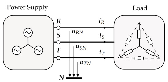
Figure 1.
Three-phase three-wire electrical circuit.
The transformation is based on the principle of isomorphism between vector spaces. In this case, the time domain periodic Fourier functions and Euclidean vector space. Thus, the basis used for the geometric transformation can be chosen as in single-phase systems [12]:
Any current or voltage variable in the time domain (including the DC component) can be expressed as a vector in the geometric domain by using dimensions, where n is the number of harmonics in
while and are the Fourier coefficients of the harmonic k and is the DC component. From now on, inter-harmonics and the DC component will not be considered for the sake of simplicity, but they can be seamlessly taken into account [11,18]. This representation cannot be obtained in the complex domain since it involves rotating vectors at different frequencies. Once the voltage and current vectors are defined, it is possible to introduce the geometric apparent power for three-phase systems as:
In (8), the sum of scalar products , with , leads to the geometric active power , which is similar to the traditional definition of P. Meanwhile, the sum of the exterior products leads to the geometric non-active power , which is similar to the traditional reactive power for a symmetric and sinusoidal voltage supply feeding a balanced load.
Other apparent power definitions based on euclidean or geometric principles can be found in the literature. For example, the RMS values of voltage and current vectors are used in [27], i.e., . Unfortunately, they exclusively rely on the concept of a norm. Therefore, they cannot fulfil the principle of energy conservation [12].
The norm (RMS value) of any geometric array can be calculated by using the norm definition [25]:
For a voltage waveform, the result is
A similar result can be obtained for the current . It can be proved that [18], i.e., the product of vector norms equals the norm of the geometric power
where the reverse of a general geometric array is defined as .
3. Case I: Balanced, Symmetric and Sinusoidal
In this section, the proposed theory is applied to a three-phase circuit that operates under balanced, symmetric and sinusoidal conditions. Although it is a well-known case, already solved in the literature, we believe it is a good example to understand the GA-based methodology. For clarification, the traditional complex algebra solution is also presented. The computations were carried out using a Matlab library kown as GAPoTNumLib developed by the some of the authors for GA in electrical engineering [28].
3.1. Current, Voltage and Impedance Calculations
A three-phase three-wire electrical circuit that consists of an ideal voltage source that feeds a balanced star-connected load is shown in Figure 2. The phase voltages are , and while the line currents are , and . These waveforms are defined in the time domain. They can be transformed to the geometric domain by using the transformation shown in (6). Since the system is balanced and sinusoidal, there is only a fundamental harmonic component, i.e., . Thus, the dimension of the geometric domain is two . Under these assumptions, the chosen basis includes one scalar, two vectors and one bivector, i.e., .
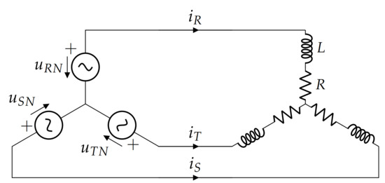
Figure 2.
Symmetrical three-phase, three-wire circuit.
The following voltage waveforms are considered:
Without loss of generality and for simplicity reasons, it is assumed that V, ° and rad/s. In this case, by virtue of (6), the geometric voltages become
which resembles the standard phasor representation in the complex domain, being the real part, and the imaginary part, as in
The Euler formula widely used in complex algebra , can also be used in GA [23]:
This exponential entity is commonly known in GA as spinor, i.e., a multivector made up of a scalar plus a bivector [29]. Any vector multiplied by a spinor undergoes a rotation of degrees in the plane defined by the bivector (in this case ) and a scaling. Therefore, spinors are commonly used to rotate elements in GA (unitary spinors are also known as rotors [24]). Note that the impedance and admittance of a passive element can also be represented as a spinor, as explained later. Hence, the voltage in (14) can be expressed in polar form as:
The reader should keep in mind that right- and left-multiplication between vectors and rotors produce rotations in opposite directions. In the rest of the paper, rotors will left-multiply vectors. In (17), it is easy to identify , and as geometric vectors in the plane -. They resemble the complex phasors , and in the complex plane, respectively. Line voltages can be calculated as follows:
Assuming an load with and H, the geometric impedance becomes:
Note that the traditional form in complex notation is . A relevant property of vectors and multivectors in GA is that the existence of an inverse is always guaranteed, provided that they are not null. For example, for a multivector in given by and a vector , their inverses are:
where
is the reverse of and is an operator that extracts the k-th grade element of . The admittance can be calculated as follows:
The currents can be found by applying Kirchhoff and Ohm’s laws to the former expressions, yielding:
Compare the results of (21) with that of complex notation , and . It may look like the complex notation is lighter than that of GA, but it comes at a cost: only two dimensions can be handled at a time, i.e., only one harmonic component can be solved. Figure 3 shows a graphical representation of geometric vectors that resembles the traditional Argand diagram for complex numbers. However, the concept of phase shift now leads to a negative angle, represented as a rotation in counter-clockwise direction. Meanwhile, phase lead is represented by a positive angle and a rotation in clockwise direction. This interesting fact can be explained by using the trigonometric identity . Therefore, we conclude that lags ( lags ).
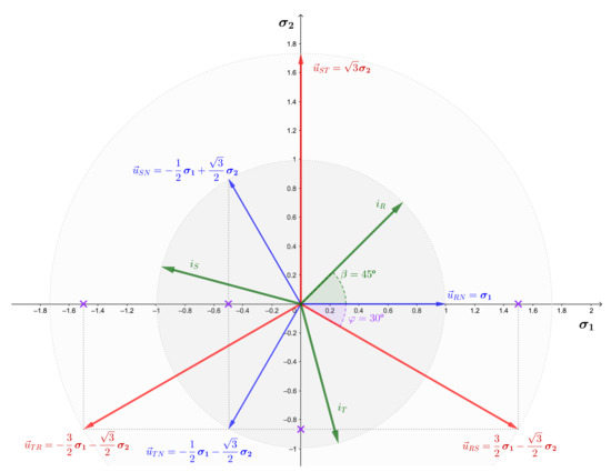
Figure 3.
Representation of voltage and current geometric vectors in the plane .
Compared to traditional complex algebra, the graphical representation of powers and impedances/admittances in GA is slightly different. These elements are spinors, i.e., entities that consist of a scalar and a bivector part. Therefore, they should not be depicted in the plane - but in the - one. It is a subtle difference, but it is worth to highlight this aspect. Although both GA objetcs and complex numbers can be depicted in Argand diagrams, completely different representations are used for GA objects, according to their nature (impedances/powers or voltages/currents). Figure 4 shows an example of a graphical representation, where the x axis now represents scalars and the y axis represents bivectors. This interpretation is a novel contribution of this paper.
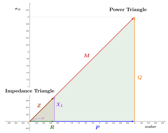
Figure 4.
Power and impedance triangle in GA plane .
3.2. Power Calculations
Therefore, the concept of three-phase geometric apparent power can be used, yielding:
where
After some algebraic manipulations, the geometric apparent power can be written as:
It can be seen that the geometric power consists of two terms of different nature. On the one hand, the active geometric power , which is a scalar number that is equal to the active power P for the sinusoidal case. Therefore, for this example, . On the other hand, we get the non-active power , which is a bivector. For the ideal case, the non-active power is equal to Q. Therefore, in this example, . Furthermore, it can be verified that yields to the same result as the traditional apparent power S by using (12):
A relevant difference between and S is that the result is a multivector and not a scalar nor a complex number, as in the traditional apparent power, . For this example (balanced and sinusoidal), the result is a spinor, where the scalar part is the active power P, while the bivector part is the well-known reactive power Q.
3.3. Current Decomposition
GA can be used to decompose currents in components that are relevant for engineering purposes (e.g., filter design), as in other power theories [6,30]. For sinusoidal single-phase circuits, the current can be decomposed into two terms: active and reactive, i.e., current in phase and in quadrature with respect to the voltage, respectively. However, if the source voltage is not sinusoidal, an additional term appears. This term is commonly known as scattered current in the CPC theory [27].
In GA, it is possible to decompose currents by applying Kirchhoff laws [31]. In the case under study, the current decomposition yields:
which can be expressed in array form as:
Therefore, the current can be decomposed into a parrallel current array (proportional to the voltage) and a quadrature current array (in quadrature with the voltage). This finding is inline with Shepherd and Zakikhany theory [4]. The squared norm of can be calculated using (9):
Note that for a balanced load, . Therefore, the active power can be written as:
Since the voltages of the system under study are balanced, then . Therefore:
Figure 5 shows a three-phase balanced circuit equivalent to that depicted in Figure 2. When these circuits are supplied with the same voltage , both demand the same active power P. In this case, the active power can be easily calculated:
Therefore, the equivalent conductance is:
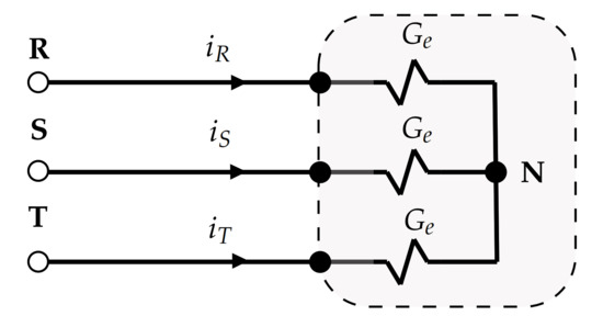
Figure 5.
Equivalent three-phase balanced resistor.
The same analysis can be carried out for the susceptance by using an equivalent load written in terms of reactances. Therefore, it is possible to derive a general expression for the equivalent admittance:
This expression simplifies the decomposition of currents into components that are significant for the engineering practice. As shown in (29), (the scalar part of ) is related to the parallel current, which, for sinusoidal systems, matches the active current, i.e., the minimum current that produces the same active power P. (the bivector part of ) is the equivalent susceptance, and leads to the quadrature current. This current does not produce net power transfer and increases the total current, thereby increasing losses. For this example, the geometric power associated to the current components can be obtained as in (8):
Compared to the traditional apparent power, the three-phase geometric apparent power defined in this work fulfills the Tellegen’s Theorem and is conservative (see references [10,11,20]) since:
3.4. Voltage Transformation Using Geometric Rotors
One of the most interesting features of GA is its ability to spatially manipulate geometric objects. For example, it is widely used in computer graphics to perform translations, reflections, or, more interestingly, rotations. In electrical engineering, a transformer can be considered as an element that causes a phase shift and a scaling of voltage or current signals between its primary and secondary terminals. This translates into a scaling and rotation in the geometrical domain, so that a voltage or current vector applied to the primary will be seen as a rotated and scaled vector in the secondary.
On the basis of the circuit in Figure 2, a three-phase transformer can be placed between the source and the load according to Figure 6. Let us assume that the transformer has a connection group Dy11. Therefore, the voltages of the secondary will be shifted by and scaled by with respect to the primary. For the symmetric case, represented by Equations (13) and (14), the time domain voltage in the secondary is
which translates to the geometric domain as
It is easy to prove that this operation corresponds to a rotation plus a scaling in the geometric domain. For this purpose, it is enough to establish the geometric object associated with the rotation, as well as the scale factor. In this way, the result can be expressed compactly in geometrical terms as
where
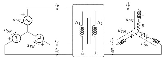
Figure 6.
Three phase circuit with a Dy11 transformer with and windings for the primary and secondary, respectively.
Note that the rotor angle is just half of the full rotation angle, because the rotation is a sandwich operation that operates half on each side of the vector. The detail of the development of (39) is as follows
4. Case II: Balanced, Symmetric and Non-Sinusoidal
In this section, the proposed theory is applied to a three-phase circuit that operates in balanced, symmetric and non-sinusoidal conditions.
4.1. Current, Voltage and Impedance Calculations
Consider again the example in Figure 2, but supplied with a non-sinusoidal, symmetric and positive sequence voltage:
Table 1 shows the well-known mapping for frequency and symmetrical sequence component depending on the harmonic order. Only three-wire systems will be considered in this work. Therefore, zero-sequence voltage and current will not be considered since it is guaranteed that they will not affect power calculations. The addition of the fourth wire is a relevant topic for further research.

Table 1.
Sequences for the different harmonic orders in a balanced three-phase system for .
Based on (6), the voltage in the geometric domain is:
where and . The current array can be calculated as in (27), yielding:
As in the sinusoidal case, it is possible to find an equivalent admittance for each of the harmonics present in the system:
4.2. Current Decomposition
The current consumed by loads is commonly decomposed for engineering purposes. The main idea is to split the current into virtual components that can be used, for example, to design and control active compensators. Current decomposition is based on Fryze’s ideas, where active and non-active currents are defined [6]. In this work, the equivalent conductance is used to calculate the active current [12]:
The current is part of , as already shown in the literature [32,33]. Therefore, the scattered current becomes:
The total current can be decomposed as follows:
The three components in the left-hand side part of (50) are in quadrature. Therefore:
4.3. Numerical Example
The circuit in Figure 2 will be analysed for the case of a non-sinusoidal symmetric voltage source such as:
where the harmonic sequences presented in Table 1 have been taken into account. The transformation to the geometric domain follows the rules presented in (6), thus
The voltage array can be expressed as:
where and are the voltages of the fundamental and the second harmonic, respectively.
The impedance for each frequency should be obtained in order to calculate the current. Since the load is balanced, then . The impedances are:
Now, the current array can be calculated as in (21):
By substituting numerical values in (54):
It can be verified that and are orthogonal since .
As the voltage and current of the load are known, the apparent geometric power can be calculated:
where
The units of active power are Watts [W] and every bivector in has units of VoltAmperes [VA]. The terms refer to the reactive power of the harmonic k, in the Budeanu’s sense [34] (voltage and current components of the same frequency that are in quadrature). The non-active power includes all the components that do not produce active power P. The active current can be obtained by using (48):
The norm of the active current is A and the norm of the total current is A. The scattered current can be calculalated by using (49):
The norm of the scattered current is A. The above results are in line with those obtained by using complex numbers (which are omitted for the sake of brevity).
Figure 7 shows the waveforms of the source voltage and several current components. The active current is proportional to the sum of the fundamental and second harmonic components of the voltage waveform. This current is part of the parallel current, along with the scattered current. It can observed that all the currents are balanced, as expected.
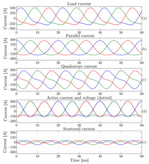
Figure 7.
Voltage and current waveforms for Example 2. (a) Load current, (b) parallel current, (c) quadrature current, (d) active current and voltage, and (e) scattered current.
5. Conclusions
In this paper, GA was applied in order to analyse and solve symmetric and balanced three-phase electrical circuits that operate under sinusoidal and non-sinusoidal conditions. The concept of geometric vector was presented in polar coordinates so that operations such as voltage and current vector rotations can easily be performed. The Argand diagram - was used to depict vectors, while the one was introduced in order to depict impedances/admittances and power components. This is a clear difference compared to traditional representations based on complex numbers. It has been shown that the proposed theory can be applied directly over three-phase electrical circuits using Kirchhoff and Ohm’s law. The use of the geometric apparent power and the current decomposition with relevant engineering meaning provide additional features compared to traditional power theories. The examples presented in the paper verify the validity of the proposed theory. Further developments will include the addition of a fourth wire and unbalanced loads under asymmetrical and distorted voltage conditions. This fact requires the use of orthogonal transformations, such as the one derived from the application of the symmetrical components. It can be addressed through the addition a higher number of dimensions.
Author Contributions
Data curation, F.M.A.-C.; Formal analysis, F.G.M. and R.B.; Investigation, F.M.A.-C.; Methodology, F.G.M. and J.R.P.; Resources, A.A.; Software, A.A.; Supervision, R.B.; Writing-–-original draft, F.G.M. and J.R.P. All authors contributed equally to this work. All authors have read and agreed to the published version of the manuscript.
Funding
This research was funded by Ministry of Science, Innovation and Universities grant number PGC2018-098813-B-C33.
Institutional Review Board Statement
Not applicable.
Informed Consent Statement
Not applicable.
Data Availability Statement
Not applicable.
Acknowledgments
This research has been supported by the Ministry of Science, Innovation and Universities at the University of Almeria under the programme “Proyectos de I+D de Generacion de Conocimiento” of the national programme for the generation of scientific and technological knowledge and strengthening of the R+D+I system with grant number PGC2018-098813-B-C33.
Conflicts of Interest
The authors declare no conflict of interest.
References
- Steinmetz, C.P. Complex quantities and their use in electrical engineering. In Proceedings of the International Electrical Congress, Chicago, IL, USA, 21–25 August 1893; pp. 33–74. [Google Scholar]
- Kennelly, A. Impedance. Trans. Am. Inst. Electr. Eng. 1893, 10, 172–232. [Google Scholar] [CrossRef]
- Heaviside, O. Electrical Papers; Macmillan and Company: New York, NY, USA, 1892; Volume 2. [Google Scholar]
- Shepherd, W.; Zand, P. Energy flow and power factor in nonsinusoidal circuits. Electron. Power 1980, 26, 263. [Google Scholar]
- Emanuel, A.E. Powers in nonsinusoidal situations—A review of definitions and physical meaning. IEEE Trans. Power Deliv. 1990, 5, 1377–1389. [Google Scholar] [CrossRef]
- Staudt, V. Fryze-Buchholz-Depenbrock: A time-domain power theory. In Proceedings of the IEEE International School on Nonsinusoidal Currents and Compensation (ISNCC 2008), Lagow, Poland, 10–13 June 2008; pp. 1–12. [Google Scholar]
- Czarnecki, L.S. Currents’ physical components (CPC) concept: A fundamental of power theory. In Proceedings of the IEEE International School on Nonsinusoidal Currents and Compensation (ISNCC 2008), Lagow, Poland, 10–13 June 2008; pp. 1–11. [Google Scholar]
- Yu, Z.; Li, D.; Zhu, S.; Luo, W.; Hu, Y.; Yuan, L. Multisource multisink optimal evacuation routing with dynamic network changes: A geometric algebra approach. Math. Methods Appl. Sci. 2018, 41, 4179–4194. [Google Scholar] [CrossRef]
- Papaefthymiou, M.; Papagiannakis, G. Real-time rendering under distant illumination with conformal geometric algebra. Math. Methods Appl. Sci. 2018, 41, 4131–4147. [Google Scholar] [CrossRef]
- Montoya, F.G.; Alcayde, A.; Arrabal-Campos, F.M.; Baños, R. Quadrature Current Compensation in Non-Sinusoidal Circuits Using Geometric Algebra and Evolutionary Algorithms. Energies 2019, 12, 692. [Google Scholar] [CrossRef]
- Montoya, F.G.; Baños, R.B.; Alcayde, A.; Arrabal-Campos, F.M. Analysis of power flow under non-sinusoidal conditions in the presence of harmonics and interharmonics using geometric algebra. Int. J. Electr. Power Energy Syst. 2019, 111, 486–492. [Google Scholar] [CrossRef]
- Montoya, F.G.; Alcayde, A.; Arrabal-Campos, F.M.; Baños, R.; Roldán-Pérez, J. Geometric Algebra Power Theory (GAPoT): Revisiting Apparent Power under Non-Sinusoidal Conditions. arXiv 2020, arXiv:2002.10011. [Google Scholar]
- Castilla, M.; Bravo, J.C.; Ordonez, M.; Montano, J.C. An approach to the multivectorial apparent power in terms of a generalized poynting multivector. Prog. Electromagn. Res. 2009, 15, 401–422. [Google Scholar] [CrossRef]
- Menti, A.; Zacharias, T.; Milias-Argitis, J. Geometric algebra: A powerful tool for representing power under nonsinusoidal conditions. IEEE Trans. Circuits Syst. I Regul. Pap. 2007, 54, 601–609. [Google Scholar] [CrossRef]
- Castro-Núñez, M.; Castro-Puche, R.; Nowicki, E. The use of geometric algebra in circuit analysis and its impact on the definition of power. In Proceedings of the IEEE 2010 International School on Nonsinusoidal Currents and Compensation (ISNCC), Lagow, Poland, 15–18 June 2010; pp. 89–95. [Google Scholar]
- Castro-Nuñez, M.; Castro-Puche, R. Advantages of geometric algebra over complex numbers in the analysis of networks with nonsinusoidal sources and linear loads. IEEE Trans. Circuits Syst. I Regul. Pap. 2012, 59, 2056–2064. [Google Scholar] [CrossRef]
- Castro-Núñez, M.; Castro-Puche, R. The IEEE Standard 1459, the CPC power theory, and geometric algebra in circuits with nonsinusoidal sources and linear loads. IEEE Trans. Circuits Syst. I Regul. Pap. 2012, 59, 2980–2990. [Google Scholar] [CrossRef]
- Montoya, F.G.; Baños, R.; Alcayde, A.; Arrabal-Campos, F.M. A new approach to single-phase systems under sinusoidal and non-sinusoidal supply using geometric algebra. Electr. Power Syst. Res. 2020, 189, 106605. [Google Scholar] [CrossRef]
- Castilla, M.; Bravo, J.C.; Ordoñez, M. Geometric algebra: A multivectorial proof of Tellegen’s theorem in multiterminal networks. IET Circuits Devices Syst. 2008, 2, 383–390. [Google Scholar] [CrossRef]
- Castilla, M.; Bravo, J.C.; Ordonez, M.; Montaño, J.C. Clifford theory: A geometrical interpretation of multivectorial apparent power. IEEE Trans. Circuits Syst. I Regul. Pap. 2008, 55, 3358–3367. [Google Scholar] [CrossRef]
- Montoya, F.G.; Roldán-Pérez, J.; Alcayde, A.; Arrabal-Campos, F.M.; Banos, R. Geometric Algebra Power Theory in Time Domain. arXiv 2020, arXiv:2002.05458. [Google Scholar]
- Lev-Ari, H.; Stanković, A.M. A geometric algebra approach to decomposition of apparent power in general polyphase networks. In Proceedings of the 41st North American Power Symposium, Starkville, MS, USA, 4–6 October 2009; pp. 1–6. [Google Scholar]
- Jancewicz, B. Multivectors and Clifford Algebra in Electrodynamics; World Scientific: Singapore, 1989. [Google Scholar]
- Dorst, L.; Fontijne, D.; Mann, S. Geometric Algebra for Computer Science: An Object-Oriented Approach to Geometry; Elsevier: Amsterdam, The Netherlands, 2010. [Google Scholar]
- Hestenes, D.; Sobczyk, G. Clifford Algebra to Geometric Calculus: A Unified Language for Mathematics and Physics; Springer Science & Business Media: Berlin/Heidelberg, Germany, 2012; Volume 5. [Google Scholar]
- Chappell, J.M.; Drake, S.P.; Seidel, C.L.; Gunn, L.J.; Iqbal, A.; Allison, A.; Abbott, D. Geometric algebra for electrical and electronic engineers. Proc. IEEE 2014, 102, 1340–1363. [Google Scholar] [CrossRef]
- Czarnecki, L.S. Currents’ Physical Components (CPC) in Circuits with Nonsinusoidal Voltages and Currents. Part 2: Three-Phase Three-Wire Linear Circuits. Electr. Power Qual. Util. J. 2006, 12, 3–13. [Google Scholar]
- Eid, A.H.; Montoya, F.G. Geometric Algebra Power Theory Numerical Library. Available online: https://github.com/ga-explorer/GAPoTNumLib (accessed on 16 March 2021).
- Hestenes, D. New Foundations for Classical Mechanics; Springer Science & Business Media: Berlin/Heidelberg, Germany, 2012; Volume 15. [Google Scholar]
- Czarnecki, L.S. Considerations on the Reactive Power in Nonsinusoidal Situations. IEEE Trans. Instrum. Meas. 1985, IM-34, 399–404. [Google Scholar] [CrossRef]
- Montoya, F.; Baños, R.; Alcayde, A.; Montoya, M.; Manzano-Agugliaro, F. Power Quality: Scientific Collaboration Networks and Research Trends. Energies 2018, 11, 2067. [Google Scholar] [CrossRef]
- Sharon, D. Reactive-power definitions and power-factor improvement in nonlinear systems. Proc. Inst. Electr. Eng. 1973, 120, 704–706. [Google Scholar] [CrossRef]
- Czarnecki, L.S. Currents’ physical components (CPC) in circuits with nonsinusoidal voltages and currents. Part 1, Single-phase linear circuits. Electr. Power Qual. Util. J. 2005, 11, 3–14. [Google Scholar]
- Willems, J.L. Budeanu’s reactive power and related concepts revisited. IEEE Trans. Instrum. Meas. 2011, 60, 1182–1186. [Google Scholar] [CrossRef]
Publisher’s Note: MDPI stays neutral with regard to jurisdictional claims in published maps and institutional affiliations. |
© 2021 by the authors. Licensee MDPI, Basel, Switzerland. This article is an open access article distributed under the terms and conditions of the Creative Commons Attribution (CC BY) license (https://creativecommons.org/licenses/by/4.0/).