Article

Deep Learning-Based Survival Analysis for High-Dimensional Survival Data

1
Department of Statistics, Pukyong National University, Busan 48513, Korea
2
Department of Artificial Intelligence Convergence, Pukyong National University, Busan 48513, Korea
*
Author to whom correspondence should be addressed.
Mathematics 2021, 9(11), 1244; https://doi.org/10.3390/math9111244
Submission received: 16 April 2021 / Revised: 18 May 2021 / Accepted: 18 May 2021 / Published: 28 May 2021

Abstract

:
With the development of high-throughput technologies, more and more high-dimensional or ultra-high-dimensional genomic data are being generated. Therefore, effectively analyzing such data has become a significant challenge. Machine learning (ML) algorithms have been widely applied for modeling nonlinear and complicated interactions in a variety of practical fields such as high-dimensional survival data. Recently, multilayer deep neural network (DNN) models have made remarkable achievements. Thus, a Cox-based DNN prediction survival model (DNNSurv model), which was built with Keras and TensorFlow, was developed. However, its results were only evaluated on the survival datasets with high-dimensional or large sample sizes. In this paper, we evaluated the prediction performance of the DNNSurv model using ultra-high-dimensional and high-dimensional survival datasets and compared it with three popular ML survival prediction models (i.e., random survival forest and the Cox-based LASSO and Ridge models). For this purpose, we also present the optimal setting of several hyperparameters, including the selection of a tuning parameter. The proposed method demonstrated via data analysis that the DNNSurv model performed well overall as compared with the ML models, in terms of the three main evaluation measures (i.e., concordance index, time-dependent Brier score, and the time-dependent AUC) for survival prediction performance.

1. Introduction

The survival time (i.e., time-to-event) is defined as the time to an event of interest, such as time-to-death, time-to-recurrence, and time-to-employment. One important characteristic of survival data is that they are often censored, which leads to incomplete outcomes. Due to the presence of censoring, statistical analysis of survival data is usually much more complicated than regular statistical analysis [1]. Many statistical methods have been developed for survival analysis by using typically non-parametric or semi-parametric statistical methods. In particular, with the development of high-throughput technologies, more and more high-dimensional (HD) or ultra-high-dimensional (ultra-HD) genomic data are being generated [2]. Unlike in regular cases, the HD case is often observed in biomedical data such as genomic data, i.e., the number of covariates (p) (e.g., gene features) is usually much larger than the sample size (n) (i.e., p n ), leading to a challenging problem [2]. In this paper, we considered the HD case, as well as the ultra-HD case where p is extremely large (e.g., p > 10 5 ).
Recently, machine learning (ML) algorithms have been widely applied for modeling nonlinear and complicated interactions, and for improving predictability, in a variety of practical fields. Therefore, they are good at handling incomplete data in survival analysis for HD survival data [3]. In particular, the neural network algorithm has been applied to survival analysis for a long time. The multilayer deep neural network (DNN) model has recently made remarkable achievements for complex and HD cases with complete data [4,5,6]. Nevertheless, the application of deep learning to survival analysis for censored data is still limited because the existing DNN survival modeling approaches only use a single hidden layer [7]. Faraggi and Simon [8] proposed a single-hidden-layer feed-forward neural network, which is usually regarded as a nonlinear extension of the Cox proportional hazards (PHs) model. However, it did not outperform the classical Cox model in a study on prostate cancer survival data [9,10]. Katzman et al. [11] restudied such a single-layer model in a deep learning framework (named DeepSurv), which showed that, in terms of Harrell’s [12] concordance index (C-index), the novel network performed better than the regular Cox model and the random survival forest [13] model in a study of breast cancer. Ching et al. [14] proposed a single-hidden-layer deep learning package (Cox-nnet) to predict patient prognosis from high-throughput omics survival data, which was also an extension of the neural network for the Cox model. It was demonstrated that the neural network survival model performed similar to or better than the regular Cox model, the penalized Cox model, and the random survival forest model using TCGA (The Cancer Genomic Atlas) cancer data with high-throughput gene expressions. To overcome such a restriction, very recently, Sun et al. [7] developed a multi-hidden-layer Cox-based DNN survival model (DNNSurv model) to predict the progression of age-related macular degeneration (AMD) disease and compared it with other survival models based on machine learning. It was shown that, in a study of AMD progression, the DNNSurv model not only outperformed several other survival models (e.g., penalized Cox model and random survival forest model) in terms of the evaluation metrics (e.g., C-index), but also successfully obtained the patient-specific predictor importance measures using the local interpretable model-agnostic explanation (LIME) method [15]. However, it was only concerned with the survival datasets with both HD and a large sample size.
In this paper, we evaluated the prediction performance of the DNNSurv model using several HD and ultra-HD datasets for survival analysis and compared it with three popular ML survival prediction models (i.e., random survival forest model and Cox-based LASSO and Ridge models). Here, we also present the optimal setting of several hyperparameters including the selection of the tuning parameter. The DNNSurv model was built with Keras [16] and TensorFlow [17] to make sure that the computation was stable and efficient. Keras is an open-source software library and is often used to define and train deep learning models. Several backends are supported by Keras, and TensorFlow was used as the backend engine of Keras. Keras contains numerous commonly used building blocks for neural networks, such as layers, activation functions, and optimizers, which makes the work much easier in terms of writing the deep neural network code. The DNNSurv model [7] is compatible with both GPUs and CPUs, via Keras and TensorFlow.
The paper is organized as follows. In Section 2, we review the machine and deep learning survival methods, including the prediction evaluation measures for survival analysis. In Section 3, we present the hyperparameter settings, together with a cross-validation procedure to find the optimal tuning parameter, and we then, assess the performance of four survival prediction models (DNNSurv, random survival forest, Cox-based LASSO, and Cox-based Ridge) using several real HD and ultra-HD survival datasets. The discussion is given in Section 4.

2. Machine and Deep Learning Methods for Survival Analysis

Let T be a non-negative continuous random variable that represents the time-to-event. The survival function and hazard function are denoted by S ( t ) and λ ( t ) , respectively. For each individual i ( i = 1 , , n ) , let T i be the survival time, and let C i be the corresponding censoring time. Then, observable random variables are given by:
Y i = min ( T i , C i ) and δ i = I ( T i C i ) ,
where δ i is the censoring indicator.
Let x = ( x 1 , , x p ) T be a vector of covariates for an individual, and let λ ( t ; x ) be the hazard function at time t for an individual with covariates x. Under the Cox PH model, the hazard function for an individual takes the form:
λ ( t ; x ) = λ 0 ( t ) exp ( x T β ) ,
where λ 0 ( t ) is the unspecified baseline hazard function at time t under x = 0 , and β = ( β 1 , , β p ) T is a vector of regression parameters corresponding to covariates x. The term x T β does not include the intercept term, and it is called the linear predictor or prognostic index. In this paper, the models applied for the analysis of HD or ultra-HD survival datasets were based on the Cox PH model except for the random survival forest (RSF) model.

2.1. Methods

For HD data (e.g., high-throughput genomic data) with p n , standard statistical methods cannot be applied directly. The same problems also occur in survival data [18]. To overcome these problems, various improved methods (e.g., penalized-based methods, random forests, and deep learning) have been developed. Below, we review the machine and deep learning methods used in the survival analysis of the HD time-to-event data.

2.1.1. Penalized Cox Models

Penalized Cox models are often used for processing HD survival data. The commonly used penalized Cox models include the Cox-based LASSO (Cox-LASSO) and Cox-based Ridge (Cox-Ridge) models [19,20], which are used for minimizing the negative partial log-likelihood of the Cox model with different penalty functions. The partial log-likelihood of the Cox model is given by:
( β ) = r D x r T β log i R r exp ( x i T β ) ,
where D is the set of all events, y r is the rth ( r = 1 , , E ) smallest distinct event time among the Y i ’s, E is the number of distinct events, x r is the corresponding covariate vector, and R r = { i : Y i y r } is the set of individuals who are at risk at time y r . We can then obtain the penalized maximum likelihood estimates of the regression parameters β corresponding to the two methods:
β ^ LASSO = arg min β ( β ) n + γ β 1 , β ^ Ridge = arg min β ( β ) n + γ β 2 2 ,
where β 1 = k = 1 p | β k | is the L 1 -norm penalty, β 2 = k = 1 p ( β k 2 ) 1 / 2 is the L 2 -norm penalty, and γ is the tuning parameter, which is used for the adjustment of regularization. In particular, there is no regularization when γ = 0 , and it tends to be more regularized when γ . Note here that the LASSO penalty performs well for selecting significant variables among a variety of genes, but the limit is that it can only select at most n variables for p n cases because of the convex optimization problem. The ridge penalty, on the other hand, is more suitable for solving multicollinearity problems among covariates, but is not appropriate for the variable selection problem [3].

2.1.2. Random Survival Forest

Breiman [21] proposed the random forest algorithm and showed that randomizing the base learning process can improve the performance of ensemble learning. Figure 1 shows a simple representation of a random forest. The random survival forest (RSF) algorithm [21] is an extension of the random forest to survival analysis with censored data. Because some parametric methods used for survival analysis are based on restrictive assumptions, the survival analysis is much more difficult. However, the RSF method handles these problems automatically. It is based on random bootstrap samples using the training dataset. For each bootstrap sample, it randomly selects candidate variables at each node of the tree when growing the trees. Moreover, the candidate variables are used to split the node that maximizes the survival difference among child nodes [13]. Note here that different from the random forest algorithm, the splitting rule of the RSF used for growing a tree should consider both the survival time and censoring indicator. For survival data, the log-rank splitting rule is often used to split nodes by maximizing the log-rank test statistic [22].
The main ideas of the RSF algorithm are growing a survival tree and building the ensemble cumulative hazard function, which is the average of the cumulative hazard functions (usually, we use the Nelson–Aalen cumulative hazard functions) [23]. The RSF is available using the “randomForestSRC” R package.

2.1.3. DNNSurv Model

The DNN model is well known for its capacity to learn complex covariate structures such as nonlinearity or interactions [24]. By the universal approximation theorem [25,26], for any continuous function g ( x ; β ) , it can be guaranteed that there is a neural network that approximates this function. Thus, the neural network algorithm can be extremely effective even if it consists of a very simple architecture such as just one single hidden layer. The DNNSurv model [7] was built by combining the DNN survival model and the regular Cox PH model, and it can be applied to the HD or ultra-HD survival datasets. The DNNSurv model was constructed as follows. The corresponding hazard function is of the form:
λ ( t ; x ) = λ 0 ( t ) e g ( x ; β ) ,
where g ( x ; β ) is an unknown function with a vector of parameters β , indicating the prognostic index that can be nonlinear. In other words, it is the extension of the linear predictor in the regular Cox PH model, and it becomes the Cox model when g ( x ; β ) = x T β . As a result, the DNNSurv model can be used for various nonlinear covariate structures [7]. Furthermore, because of the presence of tied events, which means that more than one event occurs from different individuals at the same time, the DNNSurv model applies Efron’s approach [27] to approximate the partial log-likelihood ( β ; x ) . It is defined by:
( β ; x ) = 1 N D r D i K r g ( x i ; β ) s = 0 k r 1 log i R r e g ( x i ; β ) s k r i K r e g ( x i ; β ) ,
where D is the set of all events with size N D , y r is the rth ( r = 1 , , E ) smallest distinct event time, K r is the set of individuals who fail at time y r , k r is the size of K r , and R r is the risk set at time y r . On the other hand, the loss function of the DNNSurv model with the L 1 penalty, which is used for handling HD covariates, is defined as:
Loss = ( β ; x ) + γ β 1 ,
where γ is the tuning parameter.
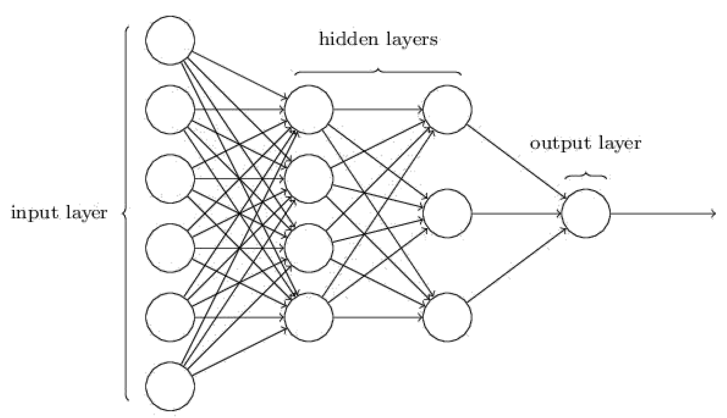
A simple structure of the DNNSurv model includes one input layer, two hidden layers, and one output layer, as shown in Figure 2. For each individual, the vector of covariates x is input into the input layer, and a scalar prognostic index g ( x ; β ) is output from the output layer with weights. For the hidden layer, the model of the lth layer can be written as a ( l ) = f ( l ) ( w 0 ( l ) + w ( l ) a ( l 1 ) ) , which is constructed by the weight w and the activation function f. The activation function of the DNNSurv model is the scaled exponential linear units (SeLUs) [28], which is defined by:
f ( x ) = a · ReLU ( x ) + λ I ( x < 0 ) b ( e x 1 ) ,
where ReLU [29] is the rectified linear unit with the form of f ( x ) = max ( 0 , x ) and a and b are constants.
The mini-batch stochastic gradient descent algorithm [30] was applied to obtain β ^ to minimize the loss function (7), and it was much faster than the standard stochastic gradient descent algorithm, in terms of minimizing the loss function. From (6) and (7), the loss function of the lth ( l = 1 , , L ) batch is given by:
l ( β ; x ) + γ β 1 .
Here,
l ( β ; x ) = 1 N D l r D l i K r l g ( x i ; β ) s = 0 k r l 1 log i R r l e g ( x i ; β ) s k r l i K r l e g ( x i ; β ) ,
where N D l , D l , K r l , k r l , and R r l are the corresponding terms for the lth batch, similar to those defined in Equation (6). Then, β can be updated through the following gradient descent formula contributed by the lth batch:
β l + 1 β l η Δ l with Δ l = β l ( β ; x ) + γ β β 1 ,
where η is the learning rate. The process is repeated n e (epoch size) times until convergence. The selection of the DNN hyperparameters, which mainly include the number of hidden layers, the number of nodes in each hidden layer, the activation function, the turning parameter, the batch size, the number of epochs, and the learning rate, is presented in detail in Section 3.

2.2. Evaluation Measures of Survival Prediction

Three popular survival accuracy metrics, i.e., the C-index, the time-dependent Brier score, and the AUC (area under the curve), were used to evaluate the performance of the survival prediction models. Below, we describe the three measures.

2.2.1. C-index

Let T 1 and T 2 be the survival times of two different subjects. The C-index [12] is defined by:
C = P T ^ 1 > T ^ 2 | T 1 > T 2 ,
where T ^ 1 and T ^ 2 are the estimated survival times of T 1 and T 2 , respectively, which can often be obtained by the estimation of the risk or prognostic scores g ( x ; β ) . It is used to measure the proportion of pairs where the predicted outcomes are concordant with the observed outcomes. The C-index can be estimated by [2,12]:
C ^ = i j δ i I ( Y i < Y j ) I g ^ ( x i ; β ^ ) > g ^ ( x j ; β ^ ) + 0.5 · I g ^ ( x i ; β ^ ) = g ^ ( x j ; β ^ ) i j δ i I ( Y i < Y j ) + I g ^ ( x i ; β ^ ) = g ^ ( x j ; β ^ ) .
The range of the value for the C-index is from 0 to 1, and a larger value indicates better performance.

2.2.2. Time-Dependent Brier Score

The definition of the time-dependent Brier score [31,32] is given by:
B S ( t ) = E I ( t ) S ( t ; x ) 2 ,
where I ( t ) = I ( T > t ) indicates the event status at time point t. The Brier score B S ( t ) indicates the mean squared error of the difference between a model-based survival function S ( t ; x ) and the event status I ( t ) . Thus, the Brier score is estimated based on the mean squared error between the predicted survival function S ^ ( t ; x i ) and the observed event status Y i ( t ) = I ( Y i > t ) at a specific time point t, where Y i = min ( T i , C i ) . The estimated Brier score [31,32] is given by:
B S ^ ( t ) = 1 n i = 1 n w i ^ ( t ) Y i ( t ) S ^ ( t ; x i ) 2 ,
where w i ^ ( t ) is the inverse probability of censoring weights (IPCW) [32], which is given by:
w i ^ ( t ) = ( 1 Y i ( t ) ) δ i G ^ ( Y i ) + Y i ( t ) G ^ ( t ) ,
where G ^ ( t ) = P ^ ( C > t ) with censoring time C and G ^ ( Y i ) indicates the estimated survival function just prior to Y i for the censoring time C. Note that the lower Brier score indicates better performance.

2.2.3. Time-Dependent AUC

The receiver operating characteristic (ROC) curve is created by plotting the true positive rate (TPR) against the false positive rate (FPR) at various threshold settings. Here, TPR and FPR were equal to sensitivity and 1-specificity, respectively. In survival analysis, the ROC depends on time t [33], with the following two definitions:
S e ( t ) = Sensitivity ( c , t ) = P M > c | T t , S p ( t ) = Specificity ( c , t ) = P M c | T > t ,
where c is an arbitrary threshold or cut-off value and M is a diagnostic test or marker (here, M = g ( x ; β ) ). The corresponding estimates of time-dependent sensitivity and specificity are given by:
S e ^ ( t ) = P g ^ ( x ; β ^ ) > c | T t , S p ^ ( t ) = P g ^ ( x ; β ^ ) c | T > t .
Therefore, we can determine the ROC curve, and furthermore, we can obtain the corresponding AUC at each time point t. The value of the AUC is between 0 and 1, and the discriminant ability is much stronger with a higher AUC.

3. Analysis of High- and Ultra-High-Dimensional Survival Data

We used both high-dimensional (HD) and ultra-HD datasets to evaluate the performance of the DNNSurv model compared with other three survival prediction models (i.e., RSF, Cox-LASSO, and Cox-Ridge).

3.1. Real Survival Datasets

We considered three datasets presented by Wang and Li [2] for the evaluation of the four survival models (i.e., DNNSurv, RSF, Cox-LASSO, and Cox-Ridge). The datasets are summarized in Table 1.
They consisted of ultra-HD (EMTAB386 and GSE49997 datasets) and HD (TCGAmirna dataset), which are available from the “curatedOvarianData” R package.
A brief introduction of the three datasets is as follows.
  • The EMTAB386 dataset contains angiogenic mRNA and microRNA gene expression signatures on 129 advanced-stage, high-grade serous ovarian cancers, which consists of 129 samples and 10357 gene features (G);
  • The GSE49997 dataset contains the expression values of 204 epithelial ovarian cancer patients, which consists of 194 samples and 16,048 gene features (G);
  • The TCGAmirna dataset contains 554 patients with high-grade serous ovarian cancer, which consists of 554 samples and 799 gene features (G).
In addition, as shown in Table 1, we also used the corresponding covariates (G + C) with both gene features (G) and clinical variables (C) in each dataset. Note that for each dataset, the time-to-event was the overall survival time, which was defined as the time from randomization to death due to any cause, and the patients who were alive or lost to follow up were censored. Before starting the survival analysis, we preprocessed all the datasets, by including the elimination of the missing values and the columns with the same values, as well as the normalization for continuous covariates.

3.2. Performance Evaluation

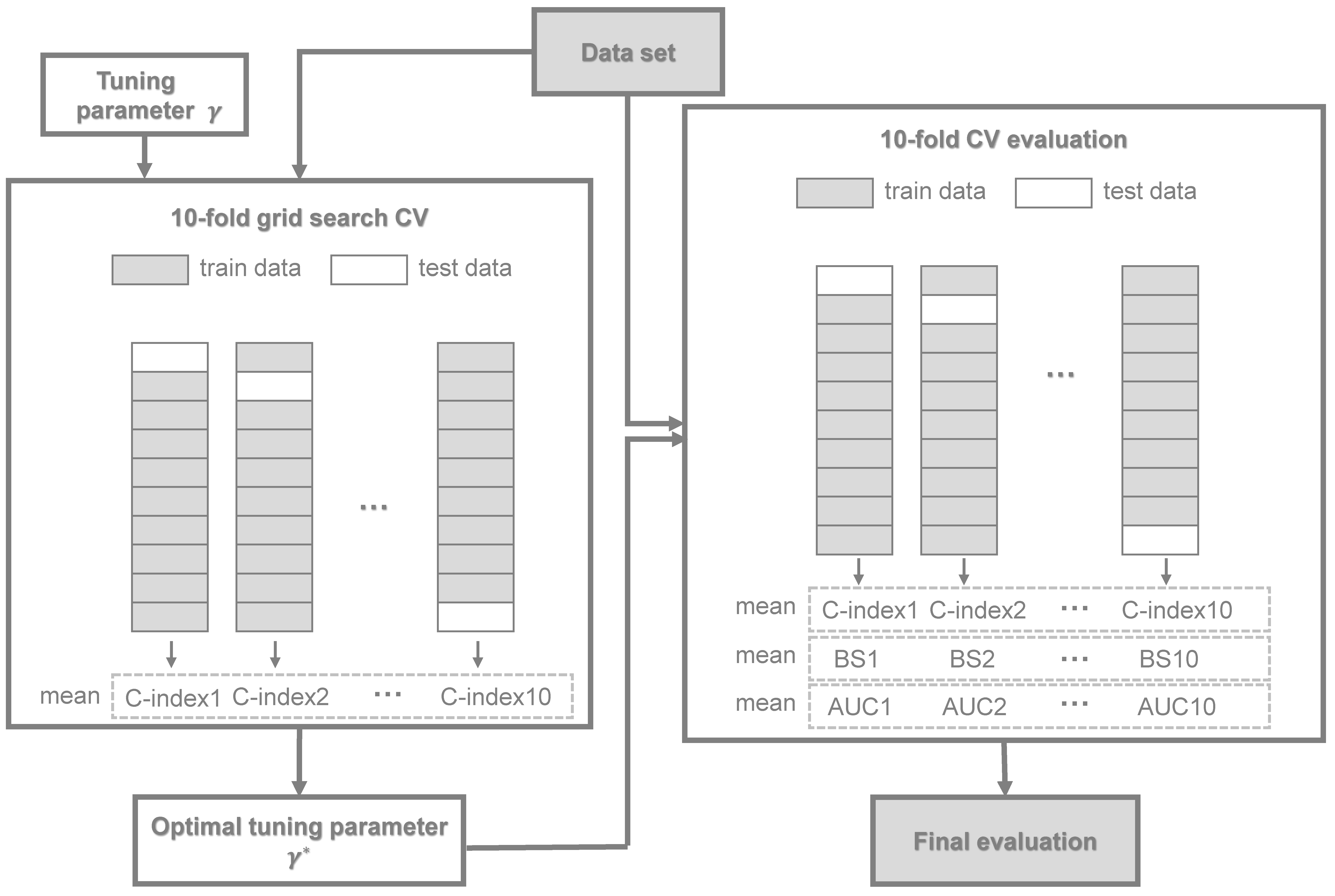
For all datasets, we evaluated the performance of the DNNSurv model using the three evaluation measures mentioned in Section 2.2 (i.e., C-index, time-dependent Brier score, and time-dependent AUC) and compared it with the performance of the other three models (i.e., RSF, Cox-LASSO, and Cox-Ridge). For the performance evaluation of all four models, a 10-fold cross-validation (CV) was performed for each real dataset in Table 1. The final results of each evaluation measure were based on the average of the results of 10 test datasets. Below, we present the 10-fold CV procedure for the four models.
  • For the DNNSurv model, (i) the first step was to perform a 10-fold CV grid search method to select an optimal tuning parameter γ * that maximizes the C-index. Here, the 10-fold CV procedure was as follows. Denote the full dataset by f, and denote the CV training and test datasets by f k ( = f f k ) and f k , respectively, for k = 1 , , 10 . For each γ and k, we found the estimator β ^ f k ( γ ) using the training dataset f k . Then, for each γ , we computed the CV estimates, i.e., C ^ ( γ ) , based on the C-index in (13):
    C ^ ( γ ) = 1 10 k = 1 10 1 M k i f k j f k δ i I ( Y i < Y j ) I g ^ k ( x i ; β ^ f k ) > g ^ k ( x j ; β ^ f k ) + 0.5 · I g ^ k ( x i ; β ^ f k ) = g ^ k ( x j ; β ^ f k ) i f k j f k δ i I ( Y i < Y j ) + I g ^ k ( x i ; β ^ f k ) = g ^ k ( x j ; β ^ f k ) .
    where M k is the sample size of the kth subset and β ^ f k = β ^ f k ( γ ) . Thus, we found the γ * (i.e., optimal tuning parameter) that maximized C ^ ( γ ) ;
    (ii) In the second step, given γ * , we performed a 10-fold CV for each dataset, i.e., we trained the model on the training dataset, then obtained the values of three measures (i.e., C-index, time-dependent AUC, and Brier score (BS)) by the test dataset.
    For further understanding of our CV procedures with (i) and (ii), a flowchart is presented in Figure 3;
  • For the RSF model, we trained the model using the log-rank splitting rule for survival analysis. The corresponding parameters we selected were as follows: the number of trees was 500; the number of variables randomly selected as candidates for splitting a node was p ; and the size of the terminal node was three;
  • For the Cox-LASSO and Cox-Ridge models, the “glmnet” R package was applied. For the L 1 penalty (in the Cox-LASSO model) and the L 2 penalty (in the Cox-Ridge model), a 10-fold CV (by the cv.glmnet() R function) was first used, respectively, in the training dataset to select the optimal tuning parameter γ * * (denoted as lambda.min in the R package) that gave the minimum mean cross-validated error (cvm). After γ * * was determined, we trained each model (Cox-LASSO or Cox-Ridge) on the training dataset and then validated each model in the test dataset.
Furthermore, we controlled the hyperparameters in order to boost the performance of the DNNSurv model. The settings of the proper hyperparameters for each type of covariate are summarized in Table 2.

3.3. Results

Figure 4 and Figure 5 show the prediction performance of the four models (i.e., DNNSurv, RSF, Cox-LASSO, and Cox-Ridge) in terms of the C-index based on 10 test datasets using the 10-fold CV. Here, the covariates of each dataset in Figure 4 and Figure 5, respectively, indicate the gene features (G) and both gene features and clinical variables (G + C). As shown in Figure 4 and Figure 5, we can see that the DNNSurv model provided the best performance compared to the other three models (i.e., RSF, Cox-LASSO, and Cox-Ridge) in terms of the C-index. In particular, we can also conclude that for each dataset, the DNNSurv model revealed better performance in Figure 5 than in Figure 4 in terms of the C-index; this means that the performance of the dataset with G + C covariates was better than that with G only.
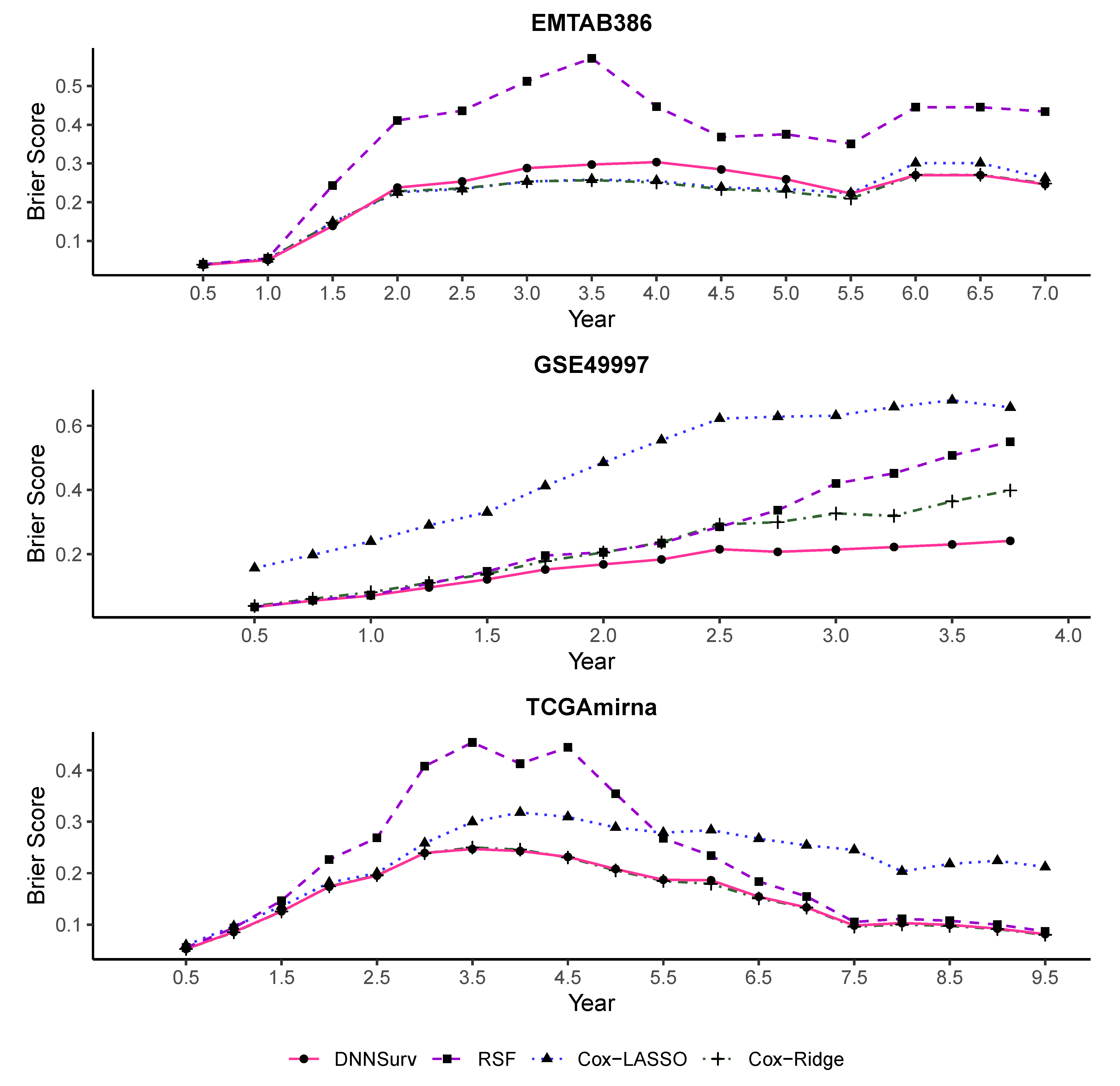
Figure 6 and Figure 7 report the performance evaluation of the four models in terms of the time-dependent Brier score on the 10 test datasets using the 10-fold CV. The difference between the two figures is that despite the gene features, there were additional clinical variables included in the datasets shown in Figure 7. As shown in Figure 6 and Figure 7, at each time point t, the value of the Brier score was the average of the results of the Brier score generated by the 10-fold CV under each model. In Figure 6 and Figure 7, the Brier score of the DNNSurv model at each time point t was consistently lower than the other three models on the GSE49997 dataset. This means that the DNNSurv model was superior compared to the other three models for this dataset. For the TCGAmirna dataset, at each time point t, the value of the Brier score for the DNNSurv model was a little smaller than the value for the other models, which means that the performance of the DNNSurv model was slightly better than the other three models in terms of the time-dependent Brier score. However, the performance of the DNNSurv model did not outperform that of the EMTAB386 dataset because it seemed that the Cox-Ridge model performed better than the DNNSurv model on this dataset. Furthermore, the overall trends of the DNNSurv model of the last two datasets from Figure 6 and Figure 7 were very similar.
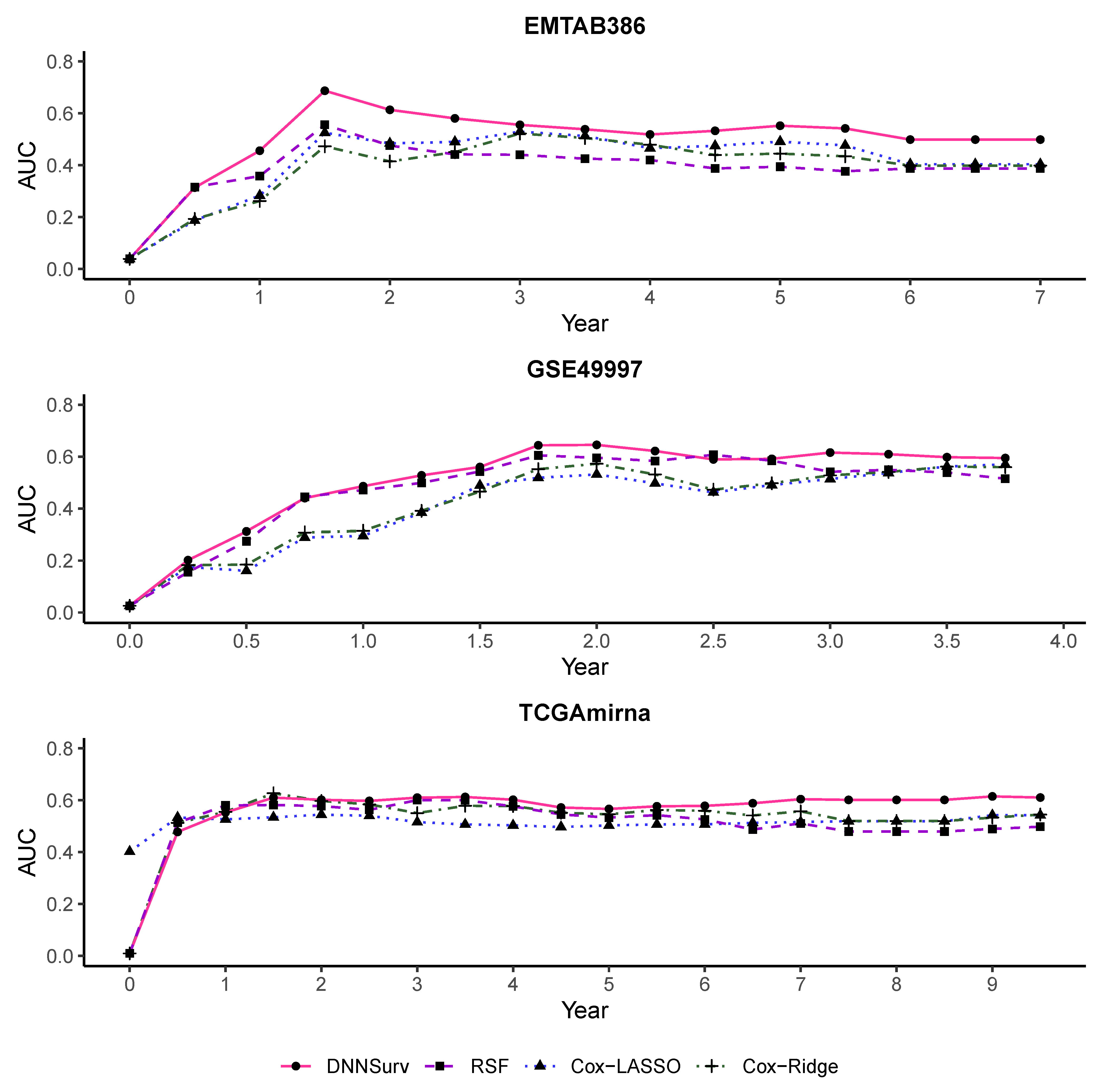
Figure 8 and Figure 9 also present the time-dependent AUC for the four models on the 10 test datasets. The structures of the datasets in Figure 8 and Figure 9 were the same as those in Figure 6 and Figure 7, respectively. For each model, the value of the AUC at each time point t was the average of the AUC at each time point t generated by the 10-fold CV. From Figure 8 and Figure 9, we can see that at almost all time points among all the datasets, the AUC values of the DNNSurv model were consistently higher than those of the other three models. The results demonstrate that the DNNSurv model performs the best in terms of the time-dependent AUC compared to the other three models (i.e., RSF, Cox-LASSO, and Cox-Ridge). Moreover, we found that for each dataset, the performance of the DNNSurv model according to the time-dependent AUC in Figure 9 was overall better than that in Figure 8.
In addition, Table 3 summarizes the 10-fold CV C-index and the Brier score and AUC at the specified time point in all four survival models under two covariate cases (G and G + C) for each dataset. Here, the results were the mean and standard deviation (SD) of the C-index and the Brier score and AUC values at 5 years for the EMTAB386 dataset, at 3.5 years for the GSE49997 dataset, and at 8.5 years for the TCGAmirna dataset, respectively, based on the 10 test datasets.
From Table 3, we found that for each of the three datasets, the performance of the DNNSurv model was overall the best among the four models in terms of the three evaluation measures. For example, for the EMTAB386 dataset, which contains the G + C case, the five-year AUC of the DNNSurv model was 0.639, which was the largest value (i.e., the best performance) among the four models. Similarly, for the GSE49997 dataset, which contains gene features only, the 3.5-year Brier score of the DNNSurv model was 0.231, which was much smaller (i.e., better performance) than the other three models (i.e., RSF, Cox-LASSO, and Cox-Ridge). According to the C-index, the DNNSurv model performed best in both the G and the G + C cases of each dataset. In particular, in terms of the C-index, for each dataset, the DNNSurv model performed better in the G + C case, which contained additional clinical variables, than in the G case. These results again confirmed the results shown in Figure 4 and Figure 5.
In summary, from Table 3 and Figure 4, Figure 5, Figure 6, Figure 7, Figure 8 and Figure 9, we can see that the DNNSurv model performed overall the best as compared to the three ML models (i.e., RSF, Cox-LASSO, and Cox-Ridge) in terms of the three evaluation measures on all the datasets we used here.

4. Discussion

In this paper, we successfully applied the DNNSurv model to real HD and ultra-HD survival datasets and effectively evaluated its ability to make accurate dynamic survival predictions. The results of the data analysis demonstrated that the DNNSurv model outperformed the three ML survival models (i.e., RSF, Cox-LASSO, and Cox-Ridge) in terms of the three evaluation measures (i.e., C-index, the time-dependent Brier score, and the AUC).
However, there were still some limitations to the DNNSurv model. For example, it took much time to run the DNNSurv model using Keras and TensorFlow. For a personal computer with an Intel Core i7-8700 3.20-GHz quad-core processor and 16 GB RAM, as an example, we took the EMTAB386 dataset, which contains gene features only. Here, the training time for the DNNSurv model was about 50 min, whereas the training times for RSF, Cox-LASSO, and Cox-Ridge were about 35 s, 5.5 s, and 3.6 s, respectively. The hyperparameter settings can be sensitive to the prediction performance. Developing a unified procedure for finding optimal hyperparameters including the tuning parameter would be interesting future work. Furthermore, an extension of the DNNsurv model to advanced survival models (e.g., the frailty model [1]) with clustered time-to-event data would also be interesting further work.

Author Contributions

L.H. and J.K. implemented the algorithms, and L.H. and S.K. conducted the data analysis. L.H. and I.D.H. wrote the initial draft, and I.D.H. verified the results and supervised this work. All authors revised the paper. All authors read and agreed to the published version of the manuscript.

Funding

This work was supported by the Basic Science Research Program through the National Research Foundation of Korea (NRF) funded by the Ministry of Education (No. NRF-2020R1F1A1A01056987).

Institutional Review Board Statement

Not applicable.

Informed Consent Statement

Not applicable.

Data Availability Statement

Publicly available datasets were analyzed in this study. These data can be found here: https://www.bioconductor.org/ (accessed on 1 April 2021).

Conflicts of Interest

The authors declare no conflict of interest.

References

  1. Ha, I.D.; Jeong, J.H.; Lee, Y. Statistical Modelling of Survival Data with Random Effects: H-Likelihood Approach; Springer: Singapore, 2017; pp. 7–104. [Google Scholar]
  2. Wang, H.; Li, G. Extreme learning machine Cox model for high-dimensional survival analysis. Stat. Med. 2019, 38, 2139–2156. [Google Scholar] [CrossRef] [PubMed]
  3. Lee, S.; Lim, H. Review of statistical methods for survival analysis using genomic data. Genom. Inform. 2019, 17, e41. [Google Scholar] [CrossRef] [PubMed]
  4. Min, S.; Lee, B.; Yoon, S. Deep learning in bioinformatics. Briefings Bioinform. 2017, 18, 851–869. [Google Scholar] [CrossRef] [Green Version]
  5. Miotto, R.; Wang, F.; Wang, S.; Jiang, X.; Dudley, J.T. Deep learning for healthcare: Review, opportunities and challenges. Briefings Bioinform. 2018, 19, 1236–1246. [Google Scholar] [CrossRef]
  6. Poplin, R.; Varadarajan, A.V.; Blumer, K.; Liu, Y.; McConnell, M.V.; Corrado, G.S.; Peng, L.; Webster, D.R. Prediction of cardiovascular risk factors from retinal fundus photographs via deep learning. Nat. Biomed. Eng. 2018, 2, 158–164. [Google Scholar] [CrossRef] [PubMed]
  7. Sun, T.; Wei, Y.; Chen, W.; Ding, Y. Genome-wide association study-based deep learning for survival prediction. Stat. Med. 2020, 39, 4605–4620. [Google Scholar] [CrossRef]
  8. Faraggi, D.; Simon, R. A neural network model for survival data. Stat. Med. 1995, 14, 73–82. [Google Scholar] [CrossRef]
  9. Xiang, A.; Lapuerta, P.; Ryutov, A.; Buckley, J.; Azen, S. Comparison of the performance of neural network methods and Cox regression for censored survival data. Comput. Stat. Data Anal. 2000, 34, 243–257. [Google Scholar] [CrossRef]
  10. Sargent, D.J. Comparison of artificial neural networks with other statistical approaches. Cancer 2001, 91, 1636–1642. [Google Scholar] [CrossRef]
  11. Katzman, J.L.; Shaham, U.; Cloninger, A.; Bates, J.; Jiang, T.; Kluger, Y. DeepSurv: Personalized treatment recommender system using a Cox proportional hazards deep neural network. BMC Med. Res. Methodol. 2018, 18, 1–12. [Google Scholar] [CrossRef]
  12. Harrell, F.E.; Lee, K.L.; Mark, D.B. Multivariable prognostic models: Issues in developing models, evaluating assumptions and adequacy, and measuring and reducing errors. Stat. Med. 1996, 15, 361–387. [Google Scholar] [CrossRef]
  13. Ishwaran, H.; Kogalur, U.B.; Blackstone, E.H.; Lauer, M.S. Random survival forests. Ann. Appl. Stat. 2008, 2, 841–860. [Google Scholar] [CrossRef]
  14. Ching, T.; Zhu, X.; Garmire, L.X. Cox-nnet: An artificial neural network method for prognosis prediction of high-throughput omics data. PLoS Comput. Biol. 2018, 14, e1006076. [Google Scholar] [CrossRef]
  15. Ribeiro, M.T.; Singh, S.; Guestrin, C. Why should i trust you? Explaining the predictions of any classifier. In Proceedings of the 22nd ACM SIGKDD International Conference on Knowledge Discovery and Data Mining, San Francisco, CA, USA, 13–17 August 2016; pp. 1135–1144. [Google Scholar]
  16. Chollet, F. Keras. GitHub. 2015. Available online: https://github.com/fchollet/keras (accessed on 18 March 2021).
  17. Abadi, M.; Barham, P.; Chen, J.; Chen, Z.; Davis, A.; Dean, J.; Devin, M.; Ghemawat, S.; Irving, G.; Isard, M.; et al. TensorFlow: A system for large-scale machine learning. In Proceedings of the 12th USENIX Symposium on Operating Systems Design and Implementation, Savannah, GA, USA, 2–4 November 2016; pp. 265–283. [Google Scholar]
  18. Witten, D.W.; Tibshirani, R. Survival analysis with high-dimensional covariates. Stat. Methods Med. Res. 2010, 19, 29–51. [Google Scholar] [CrossRef] [PubMed]
  19. Tibshirani, R. The lasso method for variable selection in the Cox model. Stat. Med. 1997, 16, 385–395. [Google Scholar] [CrossRef] [Green Version]
  20. Hoerl, A.; Kennard, R. Ridge regression. Encycl. Stat. Sci. 2006, 8, 129–136. [Google Scholar]
  21. Breiman, L. Random forests. Mach. Learn. 2001, 45, 5–32. [Google Scholar] [CrossRef] [Green Version]
  22. Segal, M.R. Regression trees for censored data. Biometrics 1988, 44, 35–47. [Google Scholar] [CrossRef]
  23. Ishwaran, H.; Kogalur, U.B.; Chen, X.; Minn, A.J. Random survival forests for high-dimensional data. Stat. Anal. Data Min. 2011, 4, 115–132. [Google Scholar] [CrossRef]
  24. LeCun, Y.; Bengio, Y.; Hinton, G. Deep learning. Nature 2015, 521, 436. [Google Scholar] [CrossRef]
  25. Cybenko, G. Approximation by superpositions of a sigmoidal function. Math. Control. Signals Syst. 1989, 2, 303–314. [Google Scholar] [CrossRef]
  26. Hornik, K.; Stinchcombe, M.; White, H. Multilayer feedforward networks are universal approximators. Neural Netw. 1989, 2, 359–366. [Google Scholar] [CrossRef]
  27. Efron, B. The efficiency of Cox’s likelihood function for censored data. J. Am. Stat. Assoc. 1977, 72, 557–565. [Google Scholar] [CrossRef]
  28. Klambauer, G.; Unterthiner, T.; Mayr, A.; Hochreiter, S. Self-normalizing neural networks. In Proceedings of the 31st International Conference on Neural Information Processing Systems, Long Beach, CA, USA, 4–9 December 2017; pp. 971–980. [Google Scholar]
  29. Sutskever, I.; Martens, J.; Dahl, G.; Hinton, G. On the importance of initialization and momentum in deep learning. In Proceedings of the International Conference on Machine Learning, Atlanta, GA, USA, 16–21 June 2013; pp. 1139–1147. [Google Scholar]
  30. Hinton, G.; Srivastava, N.; Swersky, K. Neural Networks for Machine Learning Lecture 6a Overview of Mini-Batch Gradient Descent; CSE 250C Machine Learning Theory Lecture; University of California: San Diego, CA, USA, 2012; p. 14. [Google Scholar]
  31. Graf, E.; Schmoor, C.; Sauerbrei, W.; Schumacher, M. Assessment and comparison of prognostic classification schemes for survival data. Stat. Med. 1999, 18, 2529–2545. [Google Scholar] [CrossRef]
  32. Gerds, T.A.; Schumacher, M. Consistent estimation of the expected Brier score in general survival models with right-censored event times. Biom. J. 2006, 48, 1029–1040. [Google Scholar] [CrossRef] [PubMed]
  33. Heagerty, P.J.; Lumley, T.; Pepe, M.S. Time-dependent ROC curves for censored survival data and a diagnostic marker. Biometrics 2000, 56, 337–344. [Google Scholar] [CrossRef] [PubMed]
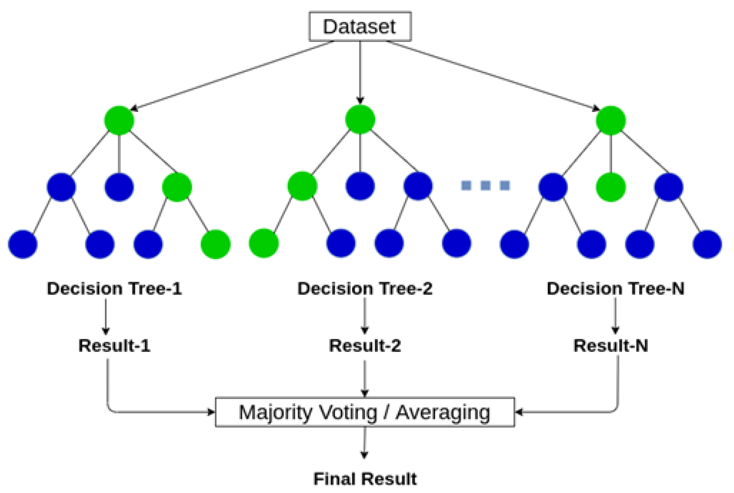
Figure 1. Diagrammatic representation of a random forest (for further details, see https://www.analyticsvidhya.com/blog/2020/05/decision-tree-vs-random-forest-algorithm/ (accessed on 1 April 2021)).
Mathematics 09 01244 g001
Figure 2. A schematic diagram of the DNNSurv structure (for further details, see https://ieeexplore.ieee.org/document/8737773) (accessed on 1 April 2021).
Mathematics 09 01244 g002
Figure 3. A flowchart of the 10-fold CV procedure of the DNNSurv model.
Mathematics 09 01244 g003
Figure 4. Boxplots of the C-index for four models on three test datasets that contain gene features only (G).
Mathematics 09 01244 g004
Figure 5. Boxplots of the C-index for four models on three test datasets that contain both gene and clinical variables (G + C).
Mathematics 09 01244 g005
Figure 6. The time-dependent Brier score for all four models on three test datasets that contain gene features only (G).
Mathematics 09 01244 g006
Figure 7. The time-dependent Brier score for all four models on three test datasets that contain both gene and clinical variables (G + C).
Mathematics 09 01244 g007
Figure 8. The time-dependent AUC for all four models on three test datasets that contain gene features only (G).
Mathematics 09 01244 g008
Figure 9. The time-dependent AUC for all four models on three test datasets that contain both gene and clinical variables (G + C).
Mathematics 09 01244 g009
Table 1. Summary of the datasets.
DatasetType of CovariatesSample Size ( n ) No. of Covariates ( p ) Censoring Rate
EMTAB386 12910,35743.4%
GSE49997G19416,04870.6%
TCGAmirna 55479947.4%
EMTAB386 10710,36244.9%
GSE49997G + C19316,05571.0%
TCGAmirna 18781432.1%
G: gene features only; G + C: gene features and clinical variables; No. of covariates: the number of covariates.
Table 2. The hyperparameter settings in the DNNSurv model for each type of covariate in the three datasets.
Type of CovariatesHyperparametersEMTAB386GSE49997TCGAmirna
No. of hidden222
No. of nodes303264
L 1 0.050.080.02
GAFSeLUSeLUSeLU
LR0.00010.00010.0001
epoch size606060
batch size484
No. of hidden222
No. of nodes503264
L 1 0.020.10.1
G + CAFSeLUSeLUSeLU
LR0.00010.00010.0001
epoch size606060
batch size888
G: gene features only; G + C: gene features and clinical variables; No. of hidden: the number of hidden layers; No. of nodes: the number of nodes per hidden layer; L 1 : tuning parameter for L 1 penalty; AF: activation function; LR: learning rate.
Table 3. The results (mean and SD) of the 10-fold CV C-index and the Brier score and AUC at the specified time point in the test data from four survival prediction models (DNNSurv, RSF, Cox-LASSO, and Cox-Ridge) for each dataset.
DatasetTypeMeasureDNNSurvRSFCox-LASSOCox-Ridge
EMTAB386 C-index (SD)0.603 (0.100)0.509 (0.102)0.499 (0.117)0.490 (0.091)
G5Y-BS (SD)0.259 (0.085)0.375 (0.171)0.234 (0.060)0.227 (0.045)
5Y-AUC (SD)0.552 (0.123)0.394 (0.187)0.491 (0.162)0.445 (0.192)
C-index (SD)0.687 (0.110)0.569 (0.102)0.488 (0.156)0.606 (0.121)
G + C5Y-BS (SD)0.334 (0.230)0.503 (0.178)0.434 (0.228)0.266 (0.160)
5Y-AUC (SD)0.639 (0.130)0.454 (0.139)0.469 (0.200)0.524 (0.158)
GSE49997 C-index (SD)0.608 (0.143)0.562 (0.149)0.448 (0.170)0.490 (0.142)
G3.5Y-BS (SD)0.231 (0.078)0.507 (0.137)0.679 (0.151)0.364 (0.088)
3.5Y-AUC (SD)0.598 (0.161)0.539 (0.137)0.562 (0.144)0.562 (0.117)
C-index (SD)0.676 (0.132)0.500 (0.190)0.567 (0.133)0.455 (0.167)
G + C3.5Y-BS (SD)0.239 (0.039)0.458 (0.253)0.320 (0.054)0.607 (0.172)
3.5Y-AUC (SD)0.588 (0.140)0.515 (0.154)0.522 (0.133)0.521 (0.192)
TCGAmirna C-index (SD)0.570 (0.092)0.552 (0.047)0.516 (0.037)0.555 (0.093)
G8.5Y-BS (SD)0.100 (0.029)0.108 (0.041)0.218 (0.290)0.098 (0.030)
8.5Y-AUC (SD)0.601 (0.124)0.479 (0.144)0.519 (0.041)0.520 (0.165)
C-index (SD)0.683 (0.079)0.566 (0.063)0.513 (0.095)0.588 (0.084)
G + C8.5Y-BS (SD)0.141 (0.060)0.156 (0.167)0.176 (0.053)0.141 (0.059)
8.5Y-AUC (SD)0.588 (0.146)0.475 (0.211)0.542 (0.148)0.483 (0.199)
Type: type of covariates; G: gene features only; G + C: gene features and clinical variables; iY-BS: i-year Brier score ( i = 3.5 , 5 , 8.5 ); iY-AUC: i-year AUC ( i = 3.5 , 5 , 8.5 ); SD: standard deviation; DNN: deep neural network; DNNSurv: Cox-based DNN survival model; RSF: random survival forest; Cox-LASSO: Cox-based LASSO; Cox-Ridge: Cox-based Ridge.
Publisher’s Note: MDPI stays neutral with regard to jurisdictional claims in published maps and institutional affiliations.