Article

On New Classes of Stancu-Kantorovich-Type Operators

by
Bianca Ioana Vasian
*,
Ștefan Lucian Garoiu
and
Cristina Maria Păcurar
Department of Mathematics and Computer Science, Faculty of Mathematics and Computer Science, Transilvania University of Brașov, Iuliu Maniu Str., 500090 Brașov, Romania
*
Author to whom correspondence should be addressed.
Mathematics 2021, 9(11), 1235; https://doi.org/10.3390/math9111235
Submission received: 14 April 2021 / Revised: 22 May 2021 / Accepted: 25 May 2021 / Published: 28 May 2021

Abstract

:
The present paper introduces new classes of Stancu–Kantorovich operators constructed in the King sense. For these classes of operators, we establish some convergence results, error estimations theorems and graphical properties of approximation for the classes considered, namely, operators that preserve the test functions e 0 ( x ) = 1 and e 1 ( x ) = x , e 0 ( x ) = 1 and e 2 ( x ) = x 2 , as well as e 1 ( x ) = x and e 2 ( x ) = x 2 . The class of operators that preserve the test functions e 1 ( x ) = x and e 2 ( x ) = x 2 is a genuine generalization of the class introduced by Indrea et al. in their paper “A New Class of Kantorovich-Type Operators”, published in Constr. Math. Anal.

1. Introduction

By C [ 0 , 1 ] , we denote the space of continuous functions defined on [ 0 , 1 ] , and by L 1 [ 0 , 1 ] , the space of all functions defined on [ 0 , 1 ] , which are Lebesgue integrable. Let N be the set of all positive integers.
We consider e j ( t ) = t j for t [ 0 , 1 ] , j N .
In order to prove Weierstrass’s approximation theorem [1], S.N. Bernstein introduced the Bernstein operators in paper [2], which, for f C [ 0 , 1 ] , are defined as:
B n ( f , x ) = k = 0 m p m , k ( x ) f k m , x [ 0 , 1 ] ,
where p m , k ( x ) = m k x k ( 1 x ) m k , for every m N , and p m , k ( x ) = 0 if k < 0 or k > m .
Let α , β 0 and α β . D. D. Stancu introduced in paper [3] the following operators, which are a generalization of the well-known Bernstein operators (see [2]), S m ( α , β ) : C α m + β , m + α m + β C [ 0 , 1 ] defined as:
S m ( α , β ) ( f , x ) = k = 0 m p m , k ( x ) f k + α m + β , x [ 0 , 1 ] ,
where p m , k ( x ) , m N , are defined as before, and f C [ 0 , 1 ] .
The Bernstein operators have been intensively studied, and many generalizations were considered, one of which is the Kantorovich variant, due to L.V. Kantorovich, from 1930 (see [4]). The Kantorovich operators K m : L 1 [ 0 , 1 ] C [ 0 , 1 ] are positive linear operators and can be defined as:
K m ( f , x ) = ( m + 1 ) k = 0 m p m , k ( x ) k m + 1 k + 1 m + 1 f ( s ) d s , x [ 0 , 1 ] ,
where p m , k ( x ) , m N , are the Bernstein basis, and f L 1 [ 0 , 1 ] .
Following the generalization of Bernstein operators proposed by Stancu, D. Bărbosu introduced in paper [5] the Kantorovich variant of Stancu–Bernstein operators, which, for f L 1 α m + β + 1 , m + α + 1 m + β + 1 , is defined as:
K m ( α , β ) ( f , x ) = ( m + β + 1 ) k = 0 m p m , k ( x ) k + α m + β + 1 k + α + 1 m + β + 1 f ( s ) d s , x [ 0 , 1 ] ,
with 0 α β , p m , k ( x ) = m k x k ( 1 x ) m k , for every m N and f L 1 [ 0 , 1 ]
The study of Kantorovich operators is still in the spotlight of many recent research papers (see [6,7,8]). Among the numerous generalizations of the Kantorovich–Bernstein type operators, we mention the one by Indrea et al., (see [9]), which introduces a new general class which preserves the test functions e 1 ( x ) and e 2 ( x ) .
In [10], J.P. King introduced a new class of positive linear Bernstein-type operators which reproduce constant functions ( e 1 ( x ) ) and e 2 ( x ) . These operators are a generalization of the Bernstein operators, but they are not polynomial-type operators. With the results introduced by King, a new direction of research was initiated, which concerns the construction of new operators with better approximation properties, obtained by modifying existing sequences of linear positive operators. This subject has been one of great interest. Gonska and Piţul (see [11]) studied estimates in terms of the first and second moduli of continuity for the operators introduced by King. Among the first generalizations of King’s result, we mention those of Agratini (see [12]), Cardena-Morales et al., (see [13]), Duman and Özarslan (see [14,15]) and Gonska et al., (see [16]). The subject is still of interest. Among the more recent studies, we mention the one by Popa (see [17]) where Voronovskaja-type theorems for King operators are studied. A recent extensive review of King type operators is that of Acar et al. (see [18]).
Based on the results in [3,9,19,20], we introduce three new classes of King-type approximation operators. The aim of our paper is to obtain convergence properties of the uniform approximation of continuous functions using a Korovkin-type theorem(see [21]). Our results are a generalization of previous results on the topic.
The article is structured as follows. Section 2 presents some known results and notions that are to be used throughout the paper. In Section 3, we introduce the general form of our operators and some properties they satisfy. In Section 4, Section 5 and Section 6, we introduced three new classes of operators, which preserve exactly two of the test functions e i , i = 0 , 1 , 2 . These operators are particular variants of the operator considered in Section 3.

2. Preliminaries

In the following, we present the notions and results that will be used to prove the main results of the paper.
We will denote by F ( I ) the set of all functions defined on I R .
Definition 1.
Let I and J be two intervals of R , such that I J . For x I , let μ x : I R , μ x ( t ) = t x , t I . For any m N , we set the functions ϕ m , k : J R , such that ϕ m , k x 0 for every x J , k { 0 , 1 , , m } and the positive linear functionals Φ m , k : U ( I ) F ( I ) R , k { 0 , 1 , , m } , where U ( I ) is a linear subspace. For m N we define the operator L m : U ( I ) F ( I ) V ( J ) F ( J ) as
L m f , x = k = 0 m ϕ m , k x Φ m , k f , x J , f U ( I ) .
Remark 1.
The operators L m m N defined above are linear and positive on U ( I ) .
Definition 2.
For i N we denote by ( Γ i L m ) the moments of order i of the operators defined in (1):
Γ i L m x = L m ( e 1 x ) i , x = k = 0 m ϕ m , k x Φ m , k ( e 1 x ) i .
Definition 3.
Let I R be a compact interval and f be continuous function on I. The modulus of continuity is a function ω f , · : [ 0 , ) R defined for any h 0 ,
ω ( f , h ) = sup { | f ( x ) f ( t ) | : x , t I , | x t | h } .
Now, let us recall the well-known result by Shisha and Mond (see [22]).
Theorem 1.
Let L be a linear positive operator on I, a compact interval. If f is a continuous function on I, then for every x I and every h > 0 , one has
| L f , x f x | | f x | · | L e 0 , x 1 | + + L e 0 , x + 1 h L e 0 , x · L ( e 0 x ) 2 , x ω f , h .
Other recent evaluations with moduli of continuity can be seen in [23].

3. A General Method for Constructing New Classes of Stancu-Type Operators

In this section, we consider a general method of constructing new types of Stancu operators, namely Stancu–Kantorovich operators with King modification. In the following sections, we will construct three new classes of such operators and we will study some properties of approximation for these operators, taking into account their expressions on the test functions e i ( t ) = t i , i = 0 , 1 , 2 , and imposing that the operators preserve two of the test functions e i and e j , i j , i , j { 0 , 1 , 2 } . A motivation for this type of modification of the operators is, as pointed out, for instance, by Acar et al., in [18], finding better properties of approximation and improved error estimates. Our approach is influenced by the modifications of Bernstein–Kantorovich operators considered in [6,9]. With this in mind, let us introduce the following operator.
Definition 4.
Let I be a compact interval and c m , d m : I R be some functions that satisfy c m x 0 , d m x 0 for all x I , 0 α β and m N . We define the following Stancu–Kantorovich type operators:
S m α , β * f , x = m + β + 1 k = 0 m m k c m x k d m x m k k + α m + β + 1 k + α + 1 m + β + 1 f t d t
for any x I , m N and f L 1 α m + β + 1 , m + α + 1 m + β + 1 .
Lemma 1.
The operator proposed in relation (3) has the following properties
S m α , β * e 0 , x = c m x + d m x m ,
S m α , β * e 1 , x = m m + β + 1 c m x c m x + d m x m 1 + 2 α + 1 2 m + β + 1 c m x + d m x m ,
S m α , β * e 2 , x = m m 1 m + β + 1 2 c m 2 x c m x + d m x m 2 + 2 m 1 + α m + β + 1 2 c m x c m x + d m x m 1 + 3 α α + 1 + 1 3 m + β + 1 2 c m x + d m x m
for any x I , m N , where e i t = t i , i { 0 , 1 , 2 } .
Proof. 
For e 0 x = 1 , we have:
S m α , β * e 0 , x = m + β + 1 k = 0 m m k c m x k d m x m k 1 m + β + 1 ,
which, from the binomial theorem, yields:
S m α , β * e 0 , x = c m x + d m x m .
Now, let us evaluate S m α , β * for e 1 x = x :
S m α , β * e 1 , x = m + β + 1 k = 0 m m k c m x k d m x m k 1 2 k + α + 1 m + β + 1 2 k + α m + β + 1 2 ,
which is
S m α , β * e 1 , x = 1 m + β + 1 k = 0 m m k k c m x k d m x m k + 2 α + 1 2 m + β + 1 c m x + d m x m .
Denoting k 1 = l in the sum from the right hand side in the above relation, we get:
S m α , β * e 1 , x = m m + β + 1 c m x l = 0 m 1 m 1 k c m x l d m x m l 1 + 2 α + 1 m + β + 1 c m x + d m x m
and, again, by the binomial theorem, we get:
S m α , β * e 1 , x = m m + β + 1 c m x c m x + d m x m 1 + 2 α + 1 m + β + 1 c m x + d m x m .
Lastly, we shall compute S m α , β * for e 2 x = x 2 :
S m α , β * e 2 , x = m + β + 1 k = 0 m m k c m x k d m x m k 1 3 k + α + 1 m + β + 1 3 k + α m + β + 1 3
Now, by doing the calculations in the square brackets, we get:
S m α , β * e 2 , x = 1 m + β + 1 2 k = 0 m m k k 2 c m x k d m x m k + 2 α + 1 m + β + 1 2 k = 0 m m k k c m x k d m x m k + 3 α α + 1 + 1 3 m + β + 1 2 c m x + d m x m .
By denoting k 2 = l in the first sum from the right hand side in the relation from above and by the binomial theorem, we will have:
S m α , β * e 2 , x = m m 1 m + β + 1 2 c m 2 x c m x + d m x m 2 + 2 m α + 1 m + β + 1 2 c m x c m x + d m x m 1 + 3 α α + 1 + 1 3 m + β + 1 2 c m x + d m x m ,
which completes the proof. □

4. Stancu–Kantorovich Type Operators Which Preserve the Functions e 0 and e 1

In this section, we shall construct an operator of Stancu–Kantorovich type as in (3), that preserves the test functions e 0 and e 1 , i.e., an operator that satisfies
S m α , β * e 0 , x = 1 S m α , β * e 1 , x = x S m α , β * e 2 , x u x 2 .
Now, from the conditions in (7) and relations (4), (5) we get
c m x = m + β + 1 m x 2 α + 1 m ,
and
d m ( x ) = m + β + 1 x m + m + 2 α + 1 m ,
for any m N and x I .
In order to have a positive operator, we shall assume that the functions c m and d m are positive. This condition yields the following inequality
2 α + 1 m + β + 1 x m + 2 α + 1 m + β + 1 , x I , m N .
Lemma 2.
For 0 2 α β and any integers m 0 < m , we have
2 α + 1 m 0 + β + 1 ; m 0 + 2 α + 1 m 0 + β + 1 2 α + 1 m + β + 1 ; m + 2 α + 1 m + β + 1 .
Proof. 
Let us consider the sequences x m m 1 ,
x m = 2 α + 1 m + β + 1
and y m m 1 ,
y m = m + 2 α + 1 m + β + 1 .
Imposing the condition 0 2 α β we have that x m m 1 is a decreasing sequence, and y m m 1 is an increasing sequence, thus implying that our inclusion holds for any m m 0 . □
Remark 2.
From now on, we will consider 0 2 α β .
Remark 3.
Since on the interval 2 α + 1 m 0 + β + 1 ; m 0 + 2 α + 1 m 0 + β + 1 we have that c m , d m 0 , for every m N , we will consider I = 2 α + 1 m 0 + β + 1 ; m 0 + 2 α + 1 m 0 + β + 1 , where m 0 is a positive integer which is arbitrarily fixed. Note that for any ε > 0 , if we make m 0 sufficiently large, then [ ε , 1 ε ] I .
Now, taking into account the sequences c m and d m obtained in (8) and (9), the operator in (3) will be
S 1 , m α , β * f , x = m + β + 1 k = 0 m m k m + β + 1 m x 2 α + 1 m k × m + β + 1 x m + m + 2 α + 1 m m k k + α m + β + 1 k + α + 1 m + β + 1 f t d t ,
for any x I .
Lemma 3.
The operator S 1 , m α , β * from (10) satisfies
S 1 , m α , β * ( e 0 , x ) = 1 ; S 1 , m α , β * ( e 1 , x ) = x ; S 1 , m α , β * ( e 2 , x ) = m 1 m x 2 + m + 2 α 1 m m + β + 1 x + 12 α α + 1 m ( 5 36 α ) 3 12 m m + β + 1 2
for x I .
Proof. 
The first two relations from (11) are obvious, and the third follows by applying relations (5), (8) and (9) and after some computations. □
Lemma 4.
The following relations hold
Γ 0 S 1 , m ( α , β ) * x = 1 ,
Γ 1 S 1 , m ( α , β ) * x = 0 ,
Γ 2 S 1 , m ( α , β ) * x = 12 m x x 2 + 24 x 2 β + 1 + 12 x 2 α + β + 36 α 5 12 m + β + 1 2 + 12 x 2 β + 1 2 + 12 x 2 α β + 2 α β 1 + 3 4 α 2 + 4 α 1 12 m m + β + 1 2 .
Proof. 
Using the previous lemma and relation (2), we get
Γ 0 S 1 , m ( α , β ) * x = 1 , Γ 1 S 1 , m ( α , β ) * x = S 1 , m ( α , β ) * e 1 , x x S 1 , m ( α , β ) * e 0 , x = 0
and
Γ 2 S 1 , m ( α , β ) * x = S 1 , m ( α , β ) * e 2 , x 2 x S 1 , m ( α , β ) * e 1 , x + x 2 S 1 , m ( α , β ) * e 0 , x = m 1 m x 2 + m + 2 α 1 m m + β + 1 x + 12 α α + 1 m ( 5 36 α ) 3 12 m m + β + 1 2 x 2 .
which, after some calculations, yields (14). □
Lemma 5.
We have
lim m m Γ 2 S 1 , m ( α , β ) * x = x 1 x
uniformly with respect to x I . Consequently, for any ε > 0 , there exists an integer m ε m 0 , sufficiently large, such that
Γ 2 S 1 , m ( α , β ) * x 1 4 + ε m ,
for any x I and m N such that m m ε .
Proof. 
The relation (15) follows from (12) and (14). The existence of m ε follows from the definition of the limit of a function and the inequality (16) follows from (15) by applying the inequality x 1 x 1 4 , which is true for every x 0 , 1 . □
Theorem 2.
Let f : 0 , 1 R be a continuous function on 0 , 1 . Then, we have
lim m S 1 , m ( α , β ) * f = f
uniformly on I and for every ε > 0 there exists m ε N such that
S 1 , m ( α , β ) * f , x f x 1 + 1 4 + ε ω f ; 1 m ,
for any x I and m N such that m m ε .
Proof. 
The Theorem from above follows from Theorem 1 by taking h = 1 m . □

Graphic Properties of Approximation

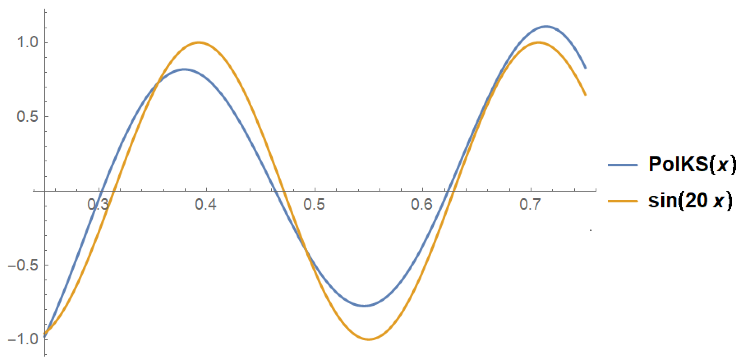
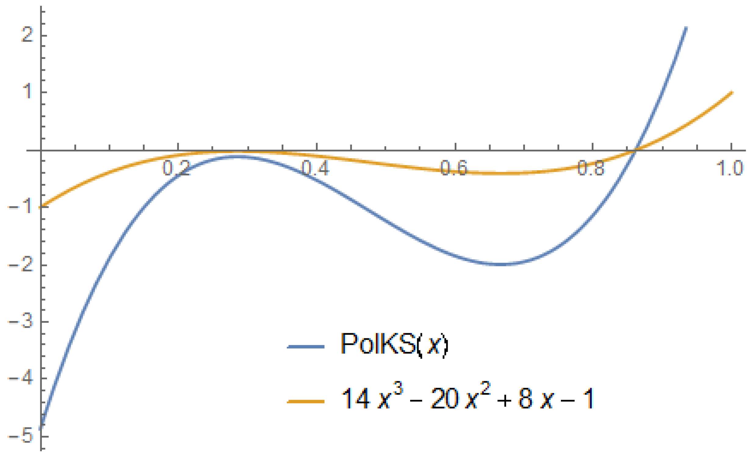
Remark 4.
It can be seen in both Figure 1 and Figure 2 that our operators approximate the given functions for α and β chosen such that α 2 β .

5. Stancu–Kantorovich-Type Operators Which Preserve the Functions e 0 and e 2

In this section, we shall construct an operator of Stancu–Kantorovich-type, as in (3), that preserves the test functions e 0 and e 2 , i.e., an operator that satisfies
S m α , β * e 0 , x = 1 S m α , β * e 2 , x = x 2 S m α , β * e 1 , x u x .
Now, imposing the condition (17) and the Equations (4) and (6), we get:
c m ( x ) + d m ( x ) = 1 , x I , m N ,
and the following quadratic equation, in c m ( x ) :
m ( m 1 ) c m 2 ( x ) + 2 m ( 1 + α ) c m ( x ) + α ( α + 1 ) + 1 3 = x 2 ( m + β + 1 ) 2 , x I , m N .
Note that for α 0 , β 0 , the discriminant
δ m ( x ) = 4 m m 2 3 + α + α 2 + α + 1 3 + x 2 ( m 1 ) ( m + β + 1 ) 2
of the quadratic Equation (19) is positive.
We make the following notation:
Δ m ( x ) = δ m ( x ) 4 .
Now, solving Equation (19) we obtain, for m 2 :
c m ( x ) = m ( 1 + α ) + Δ m ( x ) m ( m 1 )
and, from relation (18) we get
d m ( x ) = m ( m + α ) Δ m ( x ) m ( m 1 ) .
In order to have positive linear operators, we shall impose that the functions c m and d m from (21) and (22) are positive. In this case, we obtain the following inequalities:
α 2 + α + 1 3 m + β + 1 x m ( m + 2 α + 1 ) + α 2 + α + 1 3 m + β + 1 .
Lemma 6.
Let 0 < ε < 1 2 be fixed. There is an integer m 0 N such that
[ ε , 1 ε ] α 2 + α + 1 3 m + β + 1 ; m ( m + 2 α + 1 ) + α 2 + α + 1 3 m + β + 1 ,
for every m N such that m m ε and α, β, satisfying α β .
Proof. 
We have that
α 2 + α + 1 3 m + β + 1 0
and
m ( m + 2 α + 1 ) + α 2 + α + 1 3 m + β + 1 1 ,
therefore, for all ε > 0 , the inclusion (23) holds. □
Remark 5.
Since the functions c m and d m are positive on the interval considered in (23), from now on, we will consider I = ε , 1 ε , for all ε > 0 and m m 0 .
Now, taking into account the sequences c m and d m obtained in (21) and (22), the operator in (3) will be
S 2 , m α , β * f , x = m + β + 1 ( m ( m 1 ) ) m k = 0 m m k m ( 1 + α ) + Δ m ( x ) k × m ( m + α ) Δ m ( x ) m k k + α m + β + 1 k + α + 1 m + β + 1 f t d t ,
for any x I and m m 0 .
Lemma 7.
The operator S 2 , m α , β * from (24) satisfies
S 2 , m α , β * ( e 0 , x ) = 1 ; S 2 , m α , β * ( e 1 , x ) = ( m + 2 α + 1 ) + 2 Δ m ( x ) 2 ( m + β + 1 ) ( m 1 ) ; S 2 , m α , β * ( e 2 , x ) = x 2 .
for x I and m m 0 .
Proof. 
The first and last relation from (25) are obvious, and the second follows by applying relations (5) and (21). □
Now, we can obtain the following result.
Lemma 8.
The following relations hold
Γ 0 S 2 , m ( α , β ) * x = 1 ,
Γ 1 S 2 , m ( α , β ) * x = x ( m + 2 α + 1 ) + 2 Δ m ( x ) 2 ( m + β + 1 ) ( m 1 ) ,
Γ 2 S 2 , m ( α , β ) * x = 2 x x ( m + 2 α + 1 ) + 2 Δ m ( x ) 2 ( m + β + 1 ) ( m 1 ) ,
for any x I and m N .
Proof. 
Using the previous lemma and the definition of the operator Γ i from (2), we get the results after some calculations. □
Lemma 9.
We have:
lim m m Γ 1 S 2 , m ( α , β ) * x = 1 2 1 x ,
lim m m Γ 2 S 2 , m ( α , β ) * x = x 1 x ,
uniformly with regard to x I . For any ε > 0 , there exists m ε > m 0 such that
Γ 2 S 2 , m ( α , β ) * x 1 m 1 4 + ε ,
for any x I and m N such that m m ε .
Proof. 
We have:
lim m m x ( m + 2 α + 1 ) + 2 Δ m ( x ) 2 ( m + β + 1 ) ( m 1 ) =
lim m 2 Δ m ( x ) 2 ( m + β + 1 ) ( m 1 ) x m m 2 2 ( m + β + 1 ) ( m 1 ) + m ( m + 2 α + 1 ) 2 ( m + β + 1 ) ( m 1 ) =
1 2 lim m Δ m ( x ) ( m + β + 1 ) ( m 1 ) x m ,
and after some calculations, we get:
lim m m x ( m + 2 α + 1 ) + 2 Δ m ( x ) 2 ( m + β + 1 ) ( m 1 ) = 1 2 ( 1 x ) .
Now, replacing the right hand side term in (27) and (28) with (32), we will get the convergences in (29) and (30). Using the definition of the limit of a function and the inequality x ( 1 x ) 1 4 , x [ 0 , 1 ] , we have that for every ε > 0 , there exists m ε N such that the inequality (31) holds, for every m m ε . □
Now, using the above results we obtain the following theorem.
Theorem 3.
Let f : 0 , 1 R be a continuous function on 0 , 1 . Then, we have
lim m S 2 , m ( α , β ) * f ( x ) = f ( x )
uniformly on I and for every ε > 0 , there exists m ε N such that
S 2 , m ( α , β ) * f ( x ) f x 1 + 1 4 + ε ω f ; 1 m ,
for any x I and m N such that m m ε .
Proof. 
The Theorem follows from relation (31) and from Theorem 1 by taking h = 1 m . □

Graphic Properties of Approximation

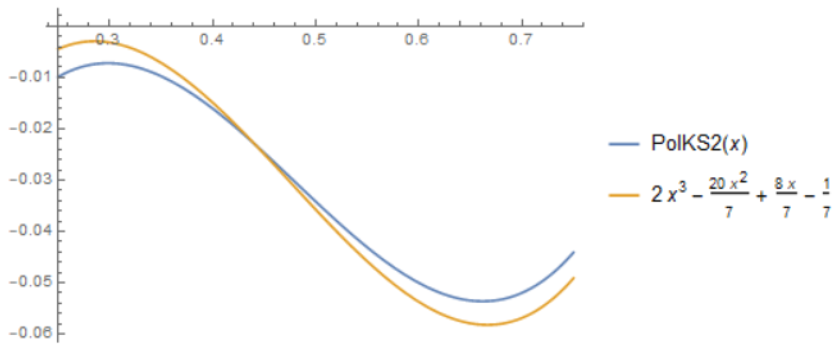
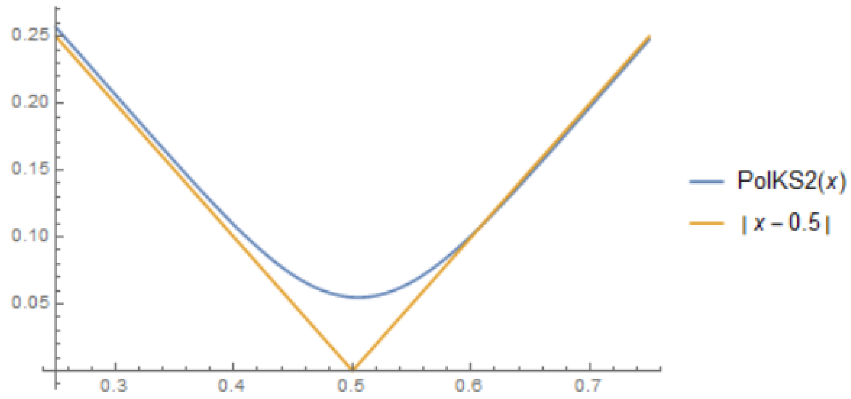
Remark 6.
Furthermore, in this case, it can be seen in Figure 3 and Figure 4 that our operators approximate the given functions.

6. Stancu–Kantorovich Type Operators Which Preserve the Functions e 1 and e 2

In this section, we shall construct an operator of Stancu–Kantorovich type as in (3), that preserves the test functions e 1 and e 2 , i.e., an operator that satisfies
S m α , β * e 0 , x u 1 S m α , β * e 1 , x = x S m α , β * e 2 , x = x 2 .
In order to obtain the main results of this section, we shall consider the following notation
S m α , β * e 0 , x = 1 + w m x ,
where x I , m N and w m : I R .
With the previous notation, we have the following remark.
Remark 7.
In order to have positive operators S m α , β * , m N , 0 α β and for the relation (34) to hold, we shall impose that S m α , β * e 0 , x 0 , which implies
1 + w m x 0 , x I , m N
From (34), we get
c m x + d m x m = 1 + w m x , x I , m N
which implies
c m x + d m x = 1 + w m x 1 m , x I , m N .
Now, from the above considerations and imposing the conditions
S m α , β * e 1 , x = x , x I , m N
and
S m α , β * e 2 , x = x 2 , x I , m N ,
we will obtain the following lemma.
Lemma 10.
We have
c m x = m + β + 1 m x 2 α + 1 2 m + β + 1 1 + w m x 1 + w m x 1 m m
and
d m x = 1 + w m x 1 m × 1 m + β + 1 m · 1 1 + w m x x 2 α + 1 2 m + β + 1 1 + w m x .
Proof. 
Equaling relations (5) and (38) , we get
m m + β + 1 c m x c m x + d m x m 1 + 2 α + 1 2 m + β + 1 c m x + d m x m = x .
Now, using the Equation (37), we have
m m + β + 1 c m x 1 + w m x m 1 m + 2 α + 1 2 m + β + 1 1 + w m x = x ,
which gives relation (40).
Now, using relations (37) and (40), by direct computation, we will get Formula (41). □
Imposing the condition (39), we will obtain the following quadratic equation in w m x :
w m 2 x 5 m 3 α 1 + m + α + w m x { 12 m m + 1 2 + β β + 2 m + 2 x 2 + 12 m + 1 2 + 2 α ( 1 + m ) + β 1 + m + 2 α x 2 5 m + 3 + 12 α 1 + m + α } + + { 12 m + 1 2 + β β + 2 m + 2 x 2 + + 12 m + 1 2 + 2 α 1 + m + β 1 + m + 2 α x 5 m + 3 + 12 α 1 + m + α } = 0 ,
which has the following solutions:
w m , 1 x = 1 2 3 5 m α m α α 2 x 2 12 m + 24 m 2 + 12 m 3 + 24 β + 24 m β + 12 β 2 + + x ( 144 144 m 24 α 24 m α 12 β 12 m β 24 α β ) + + 6 + 10 m + 24 α + 24 m α + 24 α 2 t 1 2 ( x ) + t 2 ( x ) w m , 2 x = 1 2 3 5 m α m α α 2 x 2 12 m + 24 m 2 + 12 m 3 + 24 β + 24 m β + 12 β 2 + + x ( 144 144 m 24 α 24 m α 12 β 12 m β 24 α β ) + + 6 + 10 m + 24 α + 24 m α + 24 α 2 + t 1 2 ( x ) + t 2 ( x )
where
t 1 ( x ) = 6 10 m 24 α 24 m α 24 α 2 + + x ( 144 + 144 m + 24 α + 24 m α + 12 β + 12 m β + 24 α β ) + + x 2 12 m 24 m 2 12 m 3 24 β 24 m β 12 β 2 ; t 2 ( x ) = 4 3 5 m 12 α 12 m α 12 α 2 3 5 m α m α α 2 + + 4 x 2 3 5 m α m α α 2 ( 144 144 m 36 β 24 m β ) + + 4 x 3 5 m α m α α 2 ( 144 + 144 m + 24 α + 24 m α + 12 β + 12 m β + 24 α β ) .
Remark 8.
It is easy to verify that lim m w m , 2 x = and lim m w m , 1 x = 0 , uniformly for x ( 0 , 1 ) .
From now on, in this section we will consider w m ( x ) = w m , 1 ( x ) .
In order to have a positive operator, the quantities c m ( x ) and d m ( x ) from relations (40) and (41) shall be positive. With that condition, we get the following inequalities:
x 2 α + 1 2 m + β + 1 1 + w m ( x ) 0 ,
and
1 m + β + 1 m · 1 1 + w m x x 2 α + 1 2 m + β + 1 1 + w m x 0 ,
for all x I , m N and 0 α β which lead to
2 m + β + 1 2 m + 2 α + 1 x 1 w m x 2 m + β + 1 2 α + 1 x 1 ,
for all x I , m N and 0 α β .
Lemma 11.
Let 0 < ε < 1 2 . Then, there exists m 0 N such that relation (42) holds for any x [ ε , 1 ε ] and m N , m m 0 .
Proof. 
We have w m 0 , uniformly on 0 , 1 , and
lim m 2 ( m + β + 1 ) 2 m + 2 α + 1 x 1 = x 1 ε ,
uniformly for x I . □
From now on, we will consider I = [ ε , 1 ε ] , with fixed 0 < ε < 1 2 .
We can write the operators in (3) as
S 3 , m α , β * f , x = m + β + 1 k = 0 m m k 1 + w m x 1 k × m + β + 1 m x 2 α + 1 2 m + β + 1 1 + w m x k × 1 m + β + 1 m 1 + w m x x 2 α + 1 2 m + β + 1 1 + w m x m k k + α m + β + 1 k + α m + β + 1 f t d t .
Lemma 12.
For x I and m N , we have
Γ 0 S 3 , m α , β * x = 1 + w m x ,
Γ 1 S 3 , m α , β * x = x w m x ,
Γ 2 S 3 , m α , β * x = x 2 w m x .
Proof. 
The proof follows immediately from relation (2) and from the conditions (38), (39). □
Theorem 4.
We have
lim m S 3 , m ( α , β ) * ( f , x ) = f ( x )
uniformly on I for every f C [ 0 , 1 ] .
Proof. 
By applying Theorem 1. □
Remark 9.
It was proved in [24] that there is no sequence of positive, linear and analytic operators L : C [ 0 , 1 ] C [ 0 , 1 ] that preserves the test functions e 1 and e 2 . Therefore, we have operators S 3 , m ( α , β ) * : C [ 0 , 1 ] C [ ε , 1 ε ] .

Graphic Properties of Approximation

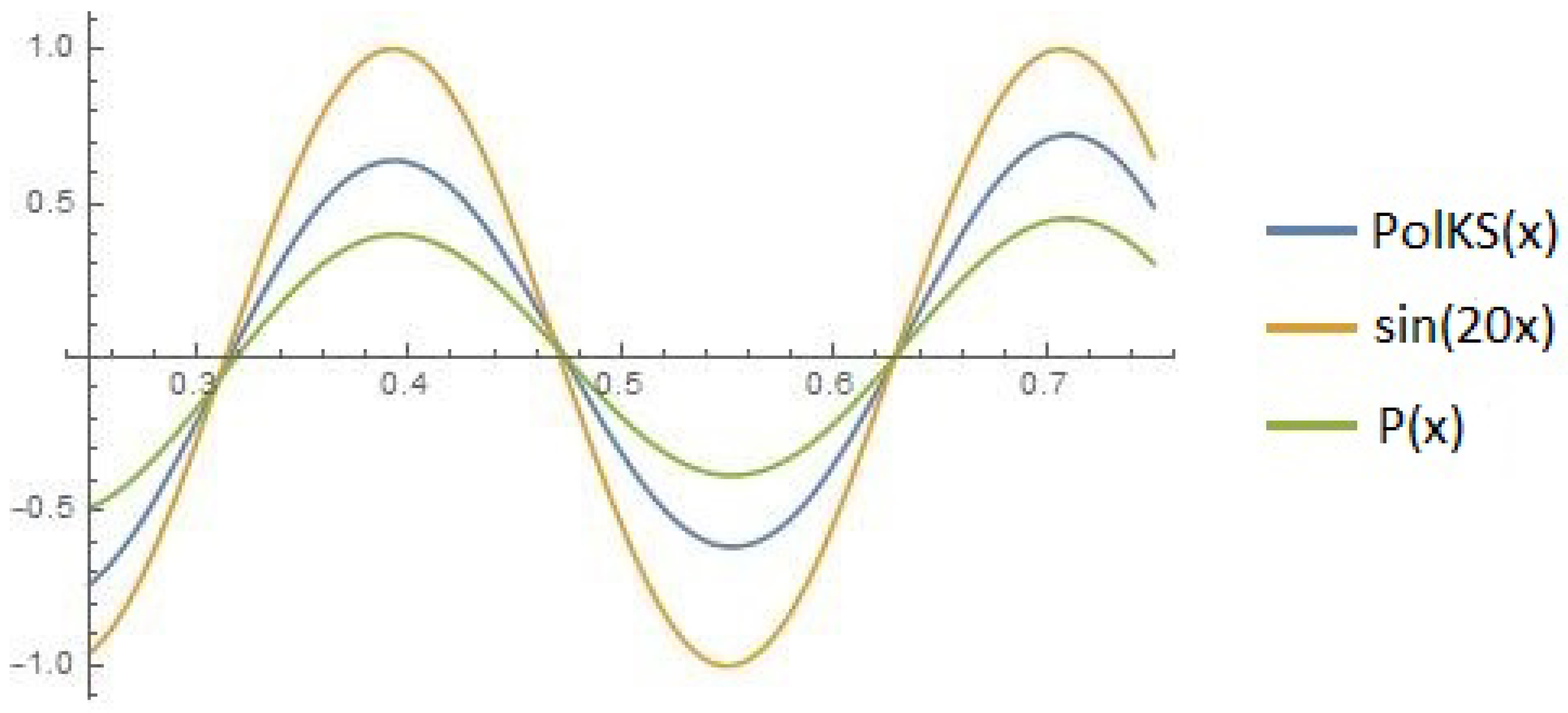
As a first comparison, we considered the function f ( x ) = sin ( 20 x ) , and we obtained the following graphics, Figure 5, where P o l K S ( x ) represents our operators that preserve e 1 and e 2 , and P ( x ) is the operator obtained by Indrea et al. in [9], which is also a particular case of our operators considered in the third section for α = β = 0 .
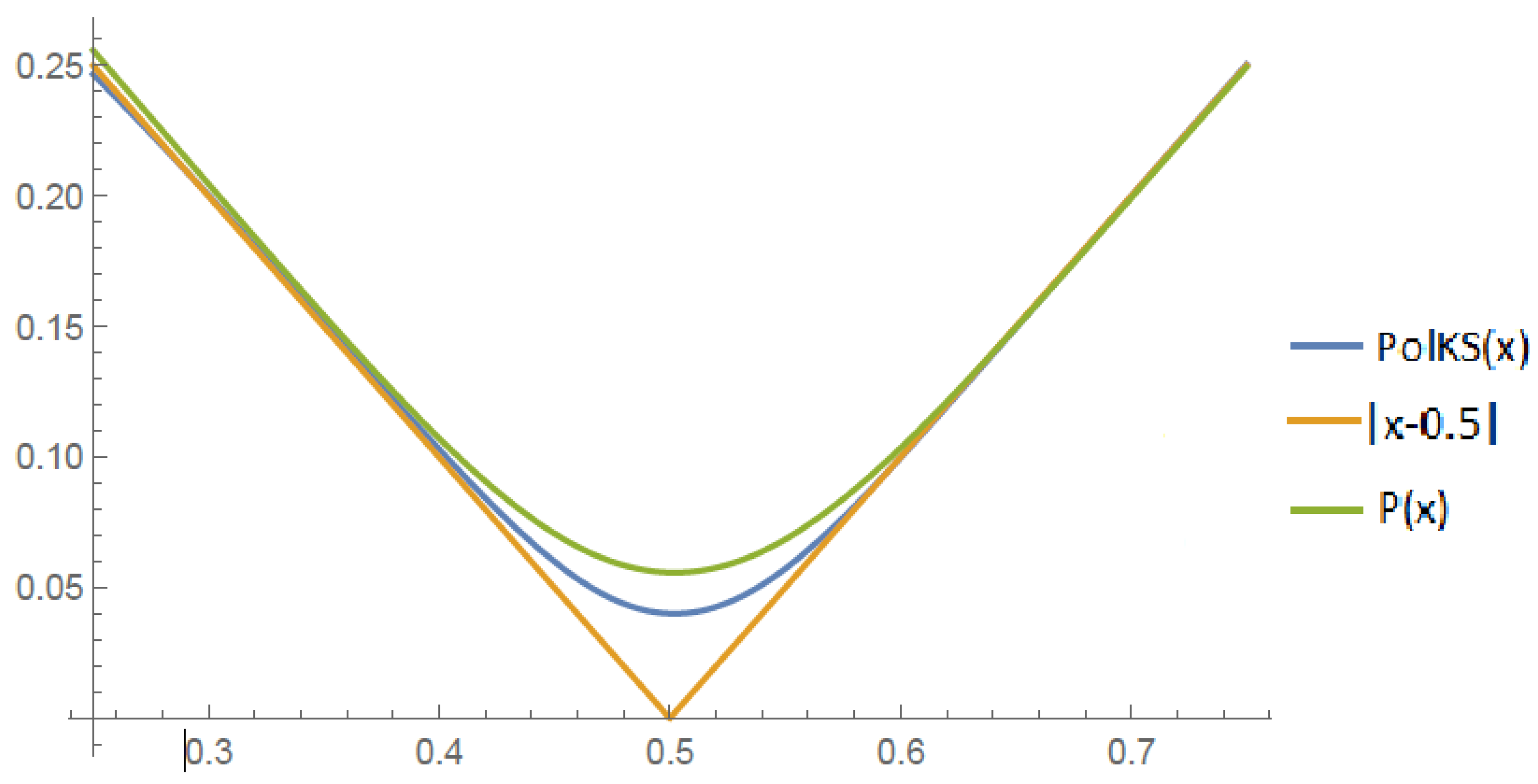
Now, we considered the function f ( x ) = | x 0.5 | and we obtained Figure 6:

Author Contributions

All authors contributed equally to this work. All authors have read and agreed to the published version of the manuscript.

Funding

The APC was funded by Transilvania University of Brașov.

Institutional Review Board Statement

Not applicable.

Informed Consent Statement

Not applicable.

Data Availability Statement

Not applicable.

Conflicts of Interest

The authors declare no conflict of interest.

References

  1. Weierstrass, K.G. Über Die Analytische Darstellbarkeit Sogenannter Willkürlicher Funktionen EinerReellen Veränderlichen, Sitzungsberichteder; Koniglich Preussischen Akademie der Wissenschcaften zu Berlin: Berlin, Germany, 1885; Volume 633–639, pp. 789–805. [Google Scholar]
  2. Bernstein, S.N. Demonstration du theoreme de Weierstrass fondee sur le calcul des probabilites. Commun. Soc. Math. Kharkov 1913, 13, 1–2. [Google Scholar]
  3. Stancu, D.D. Asupra unei generalizări a polinoamelor lui Bernstein. Stud. Univ. Babes-Bolyai Ser. Math. Phys. 1969, 14, 31–45. [Google Scholar]
  4. Kantorovich, L.V. Sur certain developpements suivant les polynomes de la forme de S. Bernstein, I, II. CR Acad. URSS 1930, 563, 595–600. [Google Scholar]
  5. Bărbosu, D. Kantorovich-Stancu type operators. J. Inequal. Pure Appl. Math. 2004, 5, 1–6. [Google Scholar]
  6. Dhamija, M.; Deo, N. Better Approximation Results by Bernstein-Kantorovich Operators. Lobachevskii J. Math. 2017, 38, 94–100. [Google Scholar] [CrossRef]
  7. Gupta, V.; Tachev, G.; Acu, A.M. Modified Kantorovich operators with better approximation properties. Numer. Algorithms 2019, 81, 125–149. [Google Scholar] [CrossRef]
  8. Hu, Y.M.; Cheng, W.T.; Gui, C.Y.; Zhang, W.H. On Stancu-Type Generalization of Modified -Szász-Mirakjan-Kantorovich Operators. J. Funct. Spaces 2021, 2021, 6683004. [Google Scholar]
  9. Indrea, A.; Indrea, A.; Pop, O. A New Class of Kantorovich-Type Operators. Constr. Math. Anal. 2020, 3, 116–124. [Google Scholar]
  10. King, J.P. Positive linear operators which preserve x2. Acta Math. Hung. 2003, 99, 203–208. [Google Scholar] [CrossRef]
  11. Gonska, H.; Piţul, P.; Rasa, I. On Peano’s form of the Taylor remainder, Voronovskaja’s theorem and the commutator of positive linear operators. In Proceedings of the International Conference on Numerical Analysis and Approximation Theory, Cluj Napoca, Romania, 5–8 July 2006; pp. 55–80. [Google Scholar]
  12. Agratini, O. Linear operators that preserve some test functions. Int. J. Math. Math. Sci. 2006, 2006, 094136. [Google Scholar] [CrossRef] [Green Version]
  13. Cardenas-Morales, D.; Garrancho, P.; Munos-Delgado, F.J. Shape preserving approximation by Bernstein-type operators which fix polinomials. Appl. Math. Comput. 2006, 182, 1615–1622. [Google Scholar] [CrossRef]
  14. Duman, O.; Özarslan, M.A. MKZ type operators providing a better estimation on [1/2,1). Can. Math. Soc. 2007, 50, 434–439. [Google Scholar]
  15. Duman, O.; Özarslan, M.A. Szász-Mirakjan type operators providing a better error estimation. Appl. Math. Lett. 2007, 20, 1184–1188. [Google Scholar] [CrossRef] [Green Version]
  16. Gonska, H.; Pitul, P. Remarks on a article of J.P. King. Comment. Math. Univ. Carol. 2005, 46, 645–652. [Google Scholar]
  17. Popa, D. Voronovskaja Type Theorems for King Type Operators. Results Math. 2020, 75, 81. [Google Scholar] [CrossRef]
  18. Acar, T.; Montano, M.C.; Garrancho, P.; Leonessa, V. On Sequences of J. P. King-Type Operators. J. Funct. Spaces 2019, 2019, 2329060. [Google Scholar] [CrossRef]
  19. Pop, O.T.; Indrea, A.D.; Braica, P.I. Durrmeyer operators of King-type. Ann. Univ. Craiova Math. Comput. Sci. Ser. 2012, 39, 288–298. [Google Scholar]
  20. Braica, P.I.; Pop, O.T.; Indrea, A.D. About a King-type operator. Appl. Math. Inf. Sci. 2012, 6, 191–197. [Google Scholar]
  21. Altomare, F.; Campiti, M. Korovkin Type Approximation Theory and its Applications. In Walter de Gruyter Studies in Mathemathics; de Gruyter & Co.: Berlin, Germany, 1994; Volume 17. [Google Scholar]
  22. Shisha, O.; Mond, B. The degree of convergence of linear positive operators. Proc. Nat. Acad. Sci. USA 1968, 60, 1196–1200. [Google Scholar] [CrossRef] [Green Version]
  23. Păltănea, R.; Smuc, M. Sharp Estimates of Asymptotic Error of Approximation by General Positive Linear Operators in Terms of the First and the Second Moduli of Continuity. Results Math. 2019, 74, 1–17. [Google Scholar] [CrossRef]
  24. Gavrea, I.; Ivan, M. A note on the fixed points of positive linear operators. J. Approx. Theory 2018, 227, 27–36. [Google Scholar] [CrossRef]
Figure 1. α = 0.1 , β = 0.2 , m = 25 iterations.
Mathematics 09 01235 g001
Figure 2. α = 0.1 , β = 0.5 , m = 500 iterations.
Mathematics 09 01235 g002
Figure 3. α = 0.1 , β = 0.65 , m = 50 iterations.
Mathematics 09 01235 g003
Figure 4. α = 0.1 , β = 0.65 , m = 50 iterations.
Mathematics 09 01235 g004
Figure 5. f ( x ) = sin ( 20 x ) , α = 10 , β = 20 , m = 50 iterations.
Mathematics 09 01235 g005
Figure 6. f ( x ) = | x 0.5 | , α = 10 , β = 20 , m = 50 iterations.
Mathematics 09 01235 g006
Publisher’s Note: MDPI stays neutral with regard to jurisdictional claims in published maps and institutional affiliations.

