Article

Robust Passivity Cascade Technique-Based Control Using RBFN Approximators for the Stabilization of a Cart Inverted Pendulum

1
Department of Electrical Engineering, Faculty of Engineering, University of Zanjan, Zanjan 45371-38791, Iran
2
Future Technology Research Center, National Yunlin University of Science and Technology, 123 University Road, Section 3, Douliou, Yunlin 64002, Taiwan
3
Department of Electrical and Computer Engineering, University of Louisiana at Lafayette, Lafayette, LA 70504-3890, USA
4
School of Electrical and Electronics Engineering, Chung-Ang University, Dongjak-gu, Seoul 06974, Korea
*
Authors to whom correspondence should be addressed.
Mathematics 2021, 9(11), 1229; https://doi.org/10.3390/math9111229
Submission received: 24 February 2021 / Revised: 6 May 2021 / Accepted: 24 May 2021 / Published: 27 May 2021
(This article belongs to the Section Engineering Mathematics)

Abstract

:
This paper proposes a novel passivity cascade technique (PCT)-based control for nonlinear inverted pendulum systems. Its main objective is to stabilize the pendulum’s upward states despite uncertainties and exogenous disturbances. The proposed framework combines the estimation properties of radial basis function neural networks (RBFNs) with the passivity attributes of the cascade control framework. The unknown terms of the nonlinear system are estimated using an RBFN approximator. The performance of the closed-loop system is further enhanced by using the integral of angular position as a virtual state variable. The lumped uncertainties (NN—Neural Network approximation, external disturbances and parametric uncertainty) are compensated for by adding a robustifying adaptive rule-based signal to the PCT-based control. The boundedness of the states is confirmed using the passivity theorem. The performance of the proposed approach was assessed using a nonlinear inverted pendulum system under both nominal and disturbed conditions.

1. Introduction

Inverted pendulums have long been considered to be interesting case studies for nonlinear control design. They owe their popularity to their inherently unstable and highly nonlinear dynamics [1,2,3]. Additionally, they have a vast range of applicability in various practical systems such as seismographs, humanoid robots, omni-wheel robots, satellite, etc. [4,5]. Various kinds of inverted pendulum systems can be found in the literature. The cart, rotational single arm and double inverted pendulum are a few examples [6,7]. In this paper, we implement our design for the cart inverted pendulum.
The stabilization of the cart inverted pendulum is a challenging task, especially when the system is subjected to model uncertainties and unknown exogenous disturbances. Various control techniques were proposed in the literature for the control and stabilization of inverted pendulum. The approach proposed in [8] combined a linear quadratic regulator (LQR) approach with a PID controller to control an inverted pendulum system. The gains of both controllers were tuned using an ant colony optimization (ANO) technique. Two fractional order PID controllers were raised in [9] for the control of a cart inverted pendulum. In [10], a sliding mode control (SMC) method was developed to achieve balance in a cart inverted pendulum system. Similarly, a second-order SMC approach was proposed in [11] for the same system. Intelligent control methods were explored in [12,13] to ensure the stability of the inverted pendulum. Besides the control approaches discussed above, in fact, the robust control of nonlinear inverted pendulum systems with matched and unmatched disturbances, which are common to many applications, remains an open problem of high practical relevance.
Cascade control has recently emerged as a potential easy to implement approach whose main property is its hierarchical structure. With the aid of cascade control, balancing of the inverted pendulum system was realized in [14]. In addition to this, the robust behavior of the closed-loop system is obtained based on active disturbance rejection technique. In [15], a cascade fuzzy controller was proposed to control the inverted pendulum system.
All the previous schemes were developed based on the Lyapunov theorem. Recently, passivity-based control has been gaining interest as a powerful tool to achieve system stabilization by passivation of the closed-loop system. Furthermore, with the use of passive property, the process of controller design is simpler. It is worth noting that some researchers have tried to find a suitable way to turn a non-passive system into a passive one, because of the value of passivity property [16,17]. Composition of passivity property and proposed controllers was reported in the literature in order to construct a robust passivity-based controller [18,19,20,21,22]. However, this control technique was seldom considered for the inverted pendulum [23].
Motivated by the above discussion, we propose a new robust passivity cascade technique, (PCT)-based control for a nonlinear inverted pendulum system subject to uncertainties. The framework of the proposed method is constructed based on cascade-RBFN technique. The main contributions of this paper are as follows:
  • A robust model-free control design formulated using RBFN approximators and passivity framework.
  • A design that enhances the performance of the closed-loop system by augmenting its dynamics with virtual states and an adaptive robustifying signal.
  • An approach that guarantees the boundedness of all the states via the output of strictly passive (OSP) property.
The remainder of the paper is organized as follows. Section 2 briefly summarizes NN approximators and the passivity theorem. The proposed controller is detailed in Section 3. Simulation results are discussed in Section 4. Some concluding remarks are finally provided in Section 5.

2. Preliminaries and Control Objectives

2.1. RBFN Approximator

In order to approximate the unknown nonlinear terms, in this study, we consider an RBFN algorithm. This latter is composed of three layers, i.e., inputs ζ = ζ 1 , ζ 2 , , ζ n T , hidden nodes and one output. Consider the Gaussian function:
h j ζ = exp ζ c j 2 2 b j 2
where j = 1 , 2 , , , n and C = c 1 , , c n . h ζ is also defined as h j ζ T . Hence, the output of RBFN can be described as:
y = θ T h x + w
where θ = θ 1 , , θ n T is derived using an adaptation mechanism.
Consider a nonlinear system in which the unknown values of g and f are estimated by a neural network system.
Lemma 1
[24]: For a set Ω , on any continuous function f ζ , there is an NN system to satisfy:
sup   x Ω   f ζ θ T h ζ w   ,   w > 0

2.2. Passivity Theorem

Definition 1
[25]: For the below nonlinear affine system:
ζ ˙ = S ζ + T ζ u   ,   ζ R n y = R ζ
Passivity property is expressed as:
π ˙ y T u
where π , y and u are, respectively, positive semidefinite function, the output and input vectors of the system. If there exists a storage function π that satisfies (6), the system (4) output is strictly passive (OSP).
π ˙ y T u y T K y
where K is a symmetric matrix with all positive eigenvalues.
Definition 2
[25]: The system (4) is zero-state observable (ZSO), if the solution ζ t 0 is the only answer of equation ζ ˙ = S ζ and R ζ = 0 .
Our control objective is to design a robust model-free controller based on the cascade technique and propose the passivity theorem framework to ensure that all closed-loop variables are bounded and the upward states are well balanced and stabilized in the presence of uncertainties.

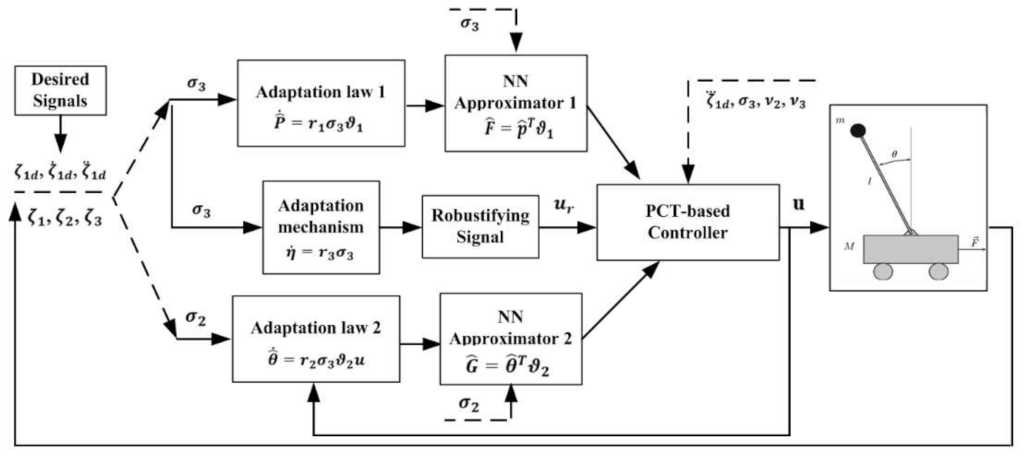
3. Proposed PCT-Based Control Design

It is well known that the system’s relative degree is one of the restrictive conditions for the passivation procedure [17,26]. Hence, in the proposed approach, we consider a cascade control technique to remove this problem.

3.1. State-Space Model of the System

In what follows, the integral of the angular joint position is added to as a virtual state to further improve the effectiveness of the system. The state-space model of the augmented system is as follows:
ζ ˙ 1 = ζ 2 ζ ˙ 2 = ζ 3 ζ ˙ 3 = f + g u + ϕ
where ζ 1 is the integral of angular position, ζ 2 denotes the angular position and ζ 3 is the angular velocity of the system. ϕ is regarded as external disturbances. f and g are also two nonlinear terms expressed as:
f = s i n ζ 2 g M + m m l ζ 3 2 c o s ζ 2 4 3 l M + m m l c o s 2 ζ 2 g = c o s ζ 2 4 3 l M + m m l c o s 2 ζ 2
To achieve the control objectives set forth, we propose the PCT-based control approach detailed in the next section.

3.2. The PCT-Based Control

Based on the cascade technique, the passivation procedure is achieved using three loops. Define the tracking errors as follows:
ν 1 = ζ 1 ζ 1 d ν 2 = ζ 2 ζ ˙ 1 d ν 3 = ζ 3 ζ ¨ 1 d
where the desired signal ζ i d is set to zero to ensure a balanced system.
Inner Loop: The first subsystem can be represented by defining σ 1 = ν 1 based on the cascade technique, as follows:
σ ˙ 1 = k 1 σ 1 + σ 2 y 1 = σ 1
in which σ 2 is a virtual input defined by: σ 2 = k 1 σ 1 + ν 2 = u 1 , whereas y 1 = σ 1 is a virtual output. Thus, system (10) is both OSP and ZSO via   π 1 :
π 1 = 0.5   σ 1 2
The time derivative of the innermost storage function yields:
π ˙ 1 = σ 1 σ ˙ 1 = k 1 σ 1 2 + σ 1 σ 2 = k 1 y 1 2 + y 1 u 1
where k 1 is a positive constant.
Middle Loop: Based on the cascade technique, the second step of design is represented as:
σ ˙ 1 = k 1 σ 1 + σ 2 σ ˙ 2 = k 2 σ 2 + σ 3 y 2 = [ σ 1   σ 2 ]
in which σ 3 = ν 3 + k 1 ν 2 + k 2 σ 2 , u 2 = σ 2   σ 3 and y 2 are, respectively, the virtual input and output of (13). Note that (13) is also OSP. This property is proven by derivative of below storage function with respect to time in the following
π 2 = π 1 + 0.5   σ 2 2
π ˙ 2 = k 1 σ 1 2 k 2 σ 2 2 + σ 1 σ 2 + σ 2 σ 3 = y 2 T u 2 y 2 T K y 2
where K = d i a g k 1 , k 2 . Based on Definition 2, It is obvious that (13) is ZSO.
Outer Loop: In the last step of design, the entire system can be introduced as:
σ ˙ 1 = k 1 σ 1 + σ 2 σ ˙ 2 = k 2 σ 2 + σ 3 σ ˙ 3 = f f ^ + g g ^ u + ϕ u r k 3 σ 3 + u p y 3 = σ 1   σ 2   σ 3
in which u r is the augmented robustifying signal and u p is the passivation control input, such that:
u p = f ^ + g ^ u + u r + k 3 σ 3 ζ 1 d + k 1 + k 2 ν 3 + k 1 k 2 ν 2
where u 3 = σ 2   σ 3   u p is the input vector of (16). In the outer loop, NN approximators are used to estimate the unknown terms. The unknown upper bound of lumped uncertainties is considered as η * . Then, η ˜ is defined as:
η ˜ = η * η
The NN approximation errors for f and g are represented as:
f f ^ = P ˜ T ϑ 1 + w 1 g g ^ = θ ˜ T ϑ 2 + w 2
where p ˜ = p p ^ (neural regressor of f), θ ˜ = θ θ ^ and w 1 and w 2 are the neural network approximation errors.
Regarding the final storage function π 3 , the OSP property of (16) is verified between π 3 and u 3 .
π 3 = π 2 + 0.5   σ 3 2 + 1 2 r 1 P ˜ T P ˜ + 1 2 r 2 θ ˜ T θ ˜ + 1 2 r 3 η ˜ 2
The time derivative of π 3 is given by:
π ˙ 3 = π ˙ 2 + σ 3 σ ˙ 3 + 1 r 1 P ˜ T P ˜ ˙ + 1 r 2 θ ˜ T θ ˜ ˙ + 1 r 3 η ˜ η ˜ ˙
Based on (16)–(21), π ˙ 3 can be simplified as:
π ˙ 3 S ˙ 2 k 3 σ 3 2 + σ 3 u p + P ˜ T 1 r 1 P ˜ ˙ + σ 3 ϑ 1 + θ ˜ T 1 r 2 θ ˜ ˙ + σ 3 ϑ 2 u + σ 3 η σ 3 u r + η ˜ 1 r 3 η ˜ ˙ + σ 3
Therefore, one can choose the adaptive rules as follows:
P ^ ˙ = r 1 σ 3 ϑ 1 θ ^ ˙ = r 2 σ 3 ϑ 2 u η ˙ = r 3 σ 3
The value of σ 3 η σ 3 u r should lead to the negative domain. Hence,
σ 3 η σ 3 u r 0     σ 3 η σ 3 u r
It is clear that:
σ 3 η σ 3 η
Thus, one can write the robustifying signal as
u r = n o r m σ 3 η  
Finally, (22) can be represented by the following equation:
π ˙ 3 π ˙ 2 k 3 σ 3 2 + σ u p
Substituting (12) and (15) into (27), one can conclude that the outer loop (16) is OSP.
π ˙ 3 y 3 T u 3 y 3 T K y 3
where K = d i a g k 1 , k 2 , k 3 . It is noteworthy to point out that (16) is ZSO due to the NN systems identifying unknown values acceptably. Moreover, the robust signal is utilized in compensation of the NN estimation errors. The block diagram of the proposed controller is shown in Figure 1.

3.3. Stability Analysis

The stability conditions for output of strictly passive systems are illustrated using Lemma 2, as follows:
Lemma 2
[25]: Consider system (4) for which the origin is assumed to be the equilibrium point. If (4) is output as strictly passive with positive definite storage function and zero-state observable (ZSO), then the origin of (4) is globally asymptotically stable for u 0 .
Based on Lemma 2, the control input for (7) is determined by replacing  u p = 0 in (17) as follows:
u = g ^ 1 f ^ + ζ 1 d k 3 σ 3 k 1 + k 2 ν 3 k 1 k 2 ν 2 u r
The asymptotic stability of (16) yields the convergence of σ 1 ,   σ 2 , σ 3 to zero. Hence, ν 1 converges to zero. The convergence of ν 2 to zero is also concluded, since ν 2 = σ 2 k 1 σ 1 . Moreover, ν 3 converges to zero, since ν 3 = σ 3 k 1 ν 2 k 2 σ 2 . Then, the boundedness of ζ 1 , ζ 2   and   ζ 3 is also guaranteed.
Remark 1:
By defining the NN approximation errors ( w 1 ζ = f ζ f ^ ( ζ | p ) , w 2 ζ = g ζ G ^ ( ζ | θ ) ) and also according to Lemma 1, the ϕ + w 1 + w 2 u m a x is equal to η , which is regarded as an optimal parameter of uncertainties.
The upper band is unknown which was derived in (23).

4. Simulation Results
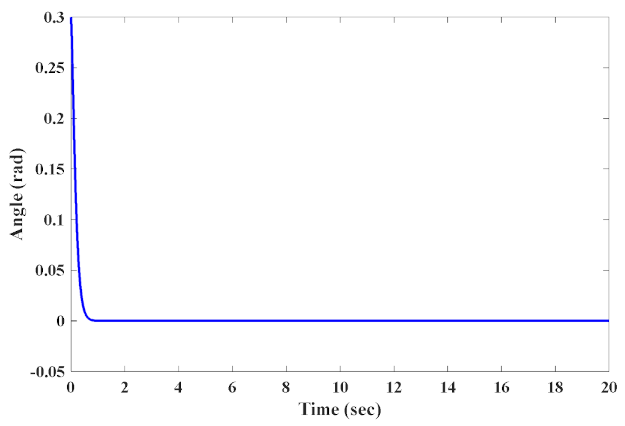
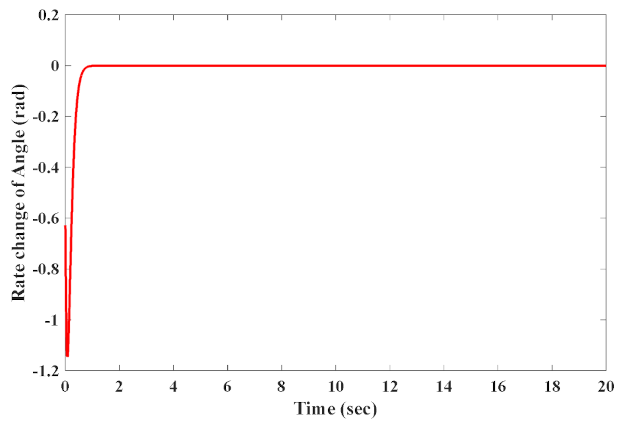
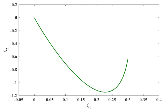
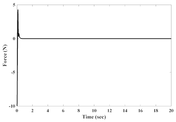
The performance of the proposed approach was assessed using the cart system inverted pendulum, the parameters of which are listed in Table 1. Two cases were considered: a normal case which assesses its performance under nomination conditions and an abnormal case which considers external disturbances (rectangular shape). In order to achieve proper tracking performance, the control parameters are fine-tuned using a trial and error approach. The obtained values are as follows:
r 1 = 10 ,   r 2 = 5 ,   r 3 = 4 k 1 = 12 ,   k 2 = 9 ,   k 3 = 6

4.1. Normal Case

The pendulum’s tracking performance under nominal conditions is illustrated in Figure 2 through Figure 5. As shown in Figure 2, the pendulum’s angle is able to perfectly track the desired position. Figure 3 and Figure 4 show the angular velocity and phase plane, respectively. From Figure 4, it is understood that the system is stable since the trajectory tends from the initial conditions to the origin. The force (control effort) applied to the system is also depicted in Figure 5. Based on the above results, it can be concluded that the pendulum’s upright states are perfectly balanced under nominal conditions.

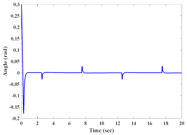
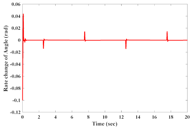
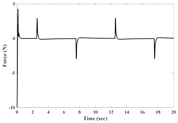
4.2. Abnormal Case (Existence of External Disturbances)

In this case, the system is subjected to the following external disturbance:
ϕ t = 10 2.5 s < t < 7.5 s ,   12.5 s < t < 17.5 s 0 o . w
The performance of the closed-loop system in this case is illustrated in Figure 6, Figure 7, Figure 8 and Figure 9.
Figure 6 and Figure 7 show the angular position and velocity of the system, respectively. The control signal is depicted in Figure 8, where the abrupt jumps refer to the shape of external disturbance. As shown in Figure 9, the phase plane trajectory of the system moves away from the origin and moves again to the origin, which indicates that the closed-loop system is stable. Finally, it can be concluded that the system has a robust behavior in the presence of a large external disturbance.

5. Conclusions

A new passivity-based cascade neural network controller was proposed in this paper to stabilize the pendulum’s upward states despite uncertainties and exogenous disturbances. The proposed approach uses RBFN approximators to estimate the system’s unknown nonlinear terms. It considers the passivity framework to design a PCT-based control approach. The lumped uncertainties are compensated for by augmenting the PCT with a robustifying adaptive rule signal. The boundedness of all the states is guaranteed via the strictly passive (OSP) property output. The controller’s performance was assessed using a nonlinear inverted pendulum system under both nominal and disturbed conditions. The obtained results confirmed the ability of the proposed approach to stabilize the pendulum’s upward states despite uncertainties and exogenous disturbances. Robustness to disturbances, acceptable tracking performance and fast response are among the positive features of the proposed approach.

Author Contributions

Conceptualization, investigation and writing—original draft preparation, R.R. and S.M.; writing—review and editing and supervision, R.R., A.F. and J.-S.R. All authors have read and agreed to the published version of the manuscript.

Funding

This research received no external funding.

Institutional Review Board Statement

Not applicable.

Informed Consent Statement

Not applicable.

Data Availability Statement

The data that support the findings of this study are available within the article.

Acknowledgments

(1) This research was supported by Basic Science Research Program through the National Research Foundation of Korea funded by the Ministry of Education (2016R1D1A1B01008058). (2) This work was supported by the Human Resources Development (No.20204030200090) of the Korea Institute of Energy Technology Evaluation and Planning (KETEP) grant funded by the Korean government Ministry of Trade, Industry and Energy.

Conflicts of Interest

The authors declare no conflict of interest.

References

  1. Mehedi, I.M.; Ansari, U.; Al-Saggaf, U. Three degrees of freedom rotary double inverted pendulum stabilization by using robust generalized dynamic inversion control: Design and experiments. J. Vib. Control. 2020, 26, 2174–2184. [Google Scholar] [CrossRef]
  2. Ben Hazem, Z.; Fotuhi, M.J.; Bingül, Z. Development of a Fuzzy-LQR and Fuzzy-LQG stability control for a double link rotary inverted pendulum. J. Frankl. Inst. 2020, 357, 10529–10556. [Google Scholar] [CrossRef]
  3. Pujol-Vazquez, G.; Mobayen, S.; Acho, L. Robust control design to the furuta system under time delay measurement feedback and exogenous-based perturbation. Mathematics 2020, 8, 2131. [Google Scholar] [CrossRef]
  4. Marinca, V.; Herisanu, N. Optimal auxiliary functions method for a pendulum wrapping on two cylinders. Mathematics 2020, 8, 1364. [Google Scholar] [CrossRef]
  5. Mobayen, S.; Tchier, F. Synchronization of A Class of Uncertain Chaotic Systems with Lipschitz Nonlinearities Using State-Feedback Control Design: A Matrix Inequality Approach. Asian J. Control. 2018, 20, 71–85. [Google Scholar] [CrossRef]
  6. Barkat, A.; Hamayun, M.T.; Ijaz, S.; Akhtar, S.; Ansari, E.A.; Ghous, I. Model identification and real-time implementation of a linear parameter–varying control scheme on lab-based inverted pendulum system. Proc. Inst. Mech. Eng. Part I J. Syst. Control. Eng. 2021, 235, 30–38. [Google Scholar] [CrossRef]
  7. Mobayen, S.; Tchier, F. Composite nonlinear feedback control technique for master/slave synchronization of nonlinear systems. Nonlinear Dyn. 2016, 87, 1731–1747. [Google Scholar] [CrossRef]
  8. Jacknoon, A.; Abido, M.A. Ant Colony based LQR and PID tuned parameters for controlling Inverted Pendulum. In Proceedings of the 2017 International Conference on Communication, Control, Computing and Electronics Engineering (ICCCCEE), Khartoum, Sudan, 16–18 January 2017; Institute of Electrical and Electronics Engineers (IEEE); Piscataway, NJ, USA, 2017; pp. 1–8. [Google Scholar]
  9. Mishra, S.K.; Chandra, D. Stabilization and Tracking Control of Inverted Pendulum Using Fractional Order PID Controllers. J. Eng. 2014, 2014, 1–9. [Google Scholar] [CrossRef] [Green Version]
  10. Elsayed, B.A.; Hassan, M.A.; Mekhilef, S. Fuzzy swinging-up with sliding mode control for third order cart-inverted pendulum system. Int. J. Control. Autom. Syst. 2014, 13, 238–248. [Google Scholar] [CrossRef] [Green Version]
  11. Mahjoub, S.; Mnif, F.; Derbel, N. Second-order sliding mode control applied to inverted pendulum. In Proceedings of the 14th International Conference on Sciences and Techniques of Automatic Control & Computer Engineering, Sousse, Tunisia, 20–22 December 2013; pp. 269–273. [Google Scholar]
  12. El-Nagar, A.M.; El-Bardini, M.; El-Rabaie, N.M. Intelligent control for nonlinear inverted pendulum based on interval type-2 fuzzy PD controller. Alex. Eng. J. 2014, 53, 23–32. [Google Scholar] [CrossRef]
  13. Jia, X.; Dai, Y.; Memon, Z.A. Adaptive Neuro-fuzzy Inference System Design of Inverted Pendulum System on an Inclined Rail. In Proceedings of the 2010 Second WRI Global Congress on Intelligent Systems, Wuhan, China, 16–17 December 2010; pp. 137–141. [Google Scholar] [CrossRef]
  14. Zhang, C.; Hu, H.; Gu, D.; Wang, J. Cascaded control for balancing an inverted pendulum on a flying quadrotor. Robotica 2017, 35, 1263–1279. [Google Scholar] [CrossRef] [Green Version]
  15. Ding, Z.; Li, Z. A cascade fuzzy control system for inverted pendulum based on Mamdani-Sugeno type. In Proceedings of the 2014 9th IEEE Conference on Industrial Electronics and Applications, Hangzhou, China, 9–11 June 2014; Institute of Electrical and Electronics Engineers (IEEE); Piscataway, NJ, USA, 2014; pp. 792–797. [Google Scholar]
  16. Byrnes, C.I.; Isidori, A.; Willems, J.C. Feedback Equivalence to Passive Nonlinear Systems. In Analysis of Controlled Dynamical Systems; J.B. Metzler: Lyon, France, 1991; pp. 118–135. [Google Scholar]
  17. Jiang, Z.-P.; Hill, D.J.; Fradkov, A.L. A passification approach to adaptive nonlinear stabilization. Syst. Control. Lett. 1996, 28, 73–84. [Google Scholar] [CrossRef]
  18. Balachandran, R.; Jorda, M.; Artigas, J.; Ryu, J.-H.; Khatib, O. Passivity-based stability in explicit force control of robots. In Proceedings of the 2017 IEEE International Conference on Robotics and Automation (ICRA), Marina Bay Sands, Singapore, 29 May–3 June 2017; pp. 386–393. [Google Scholar]
  19. Focchi, M.; Medrano-Cerda, G.A.; Boaventura, T.; Frigerio, M.; Semini, C.; Buchli, J.; Caldwell, D.G. Robot impedance control and passivity analysis with inner torque and velocity feedback loops. Control. Theory Technol. 2016, 14, 97–112. [Google Scholar] [CrossRef] [Green Version]
  20. Kostarigka, A.K.; Rovithakis, G.A. Approximate Adaptive Output Feedback Stabilization via Passivation of MIMO Uncertain Systems Using Neural Networks. IEEE Trans. Syst. Man Cybern. Part B (Cybernetics) 2009, 39, 1180–1191. [Google Scholar] [CrossRef] [PubMed]
  21. Kuntanapreeda, S. Adaptive control of fractional-order unified chaotic systems using a passivity-based control approach. Nonlinear Dyn. 2016, 84, 2505–2515. [Google Scholar] [CrossRef]
  22. Leite, A.C.; Lizarralde, F. Passivity-based adaptive 3D visual servoing without depth and image velocity measurements for uncertain robot manipulators. Int. J. Adapt. Control. Signal Process. 2016, 30, 1269–1297. [Google Scholar] [CrossRef]
  23. Haddad, N.K.; Chemori, A.; Belghith, S. Robustness enhancement of IDA-PBC controller in stabilising the inertia wheel inverted pendulum: Theory and real-time experiments. Int. J. Control. 2018, 91, 2657–2672. [Google Scholar] [CrossRef] [Green Version]
  24. Sanner, R.M.; Slotine, J.-J.E. Direct adaptive control using Gaussian networks. Nonlinear Systems Lab., MIT. Tech. Rep. SL-910303 1991.
  25. Vidyasagar, M. Nonlinear Systems Analysis; SIAM: Philadelphia, PA, USA, 2002. [Google Scholar]
  26. Lin, W. Global asymptotic stabilization of general nonlinear systems with stable free dynamics via passivity and bounded feedback. Automatica 1996, 32, 915–924. [Google Scholar] [CrossRef]
Figure 1. Schematic of the PCT-based control approach.
Mathematics 09 01229 g001
Figure 2. The pendulum angle (case 1).
Mathematics 09 01229 g002
Figure 3. The angular velocity (case 1).
Mathematics 09 01229 g003
Figure 4. The phase plane trajectory (case 1).
Mathematics 09 01229 g004
Figure 5. The control signal (case 1).
Mathematics 09 01229 g005
Figure 6. Pendulum angle (case 2).
Mathematics 09 01229 g006
Figure 7. Angular velocity (case 2).
Mathematics 09 01229 g007
Figure 8. The control signal (case 2).
Mathematics 09 01229 g008
Figure 9. Phase plane trajectory (case 2).
Mathematics 09 01229 g009
Table 1. The inverted pendulum parameters.
SymbolParameterValue
m Mass of pendulum0.2
M Mass of cart0.5
l Half-length of pendulum0.5
g Gravity acceleration9.8
Publisher’s Note: MDPI stays neutral with regard to jurisdictional claims in published maps and institutional affiliations.

