Combinatorial Models of the Distribution of Prime Numbers

Abstract

This work is divided into two parts. In the first one, the combinatorics of a new class of randomly generated objects, exhibiting the same properties as the distribution of prime numbers, is solved and the probability distribution of the combinatorial counterpart of the n-th prime number is derived together with an estimate of the prime-counting function $\pi (x)$. A proposition equivalent to the Prime Number Theorem (PNT) is proved to hold, while the equivalent of the Riemann Hypothesis (RH) is proved to be false with probability 1 (w.p. 1) for this model. Many identities involving Stirling numbers of the second kind and harmonic numbers are found, some of which appear to be new. The second part is dedicated to generalizing the model to investigate the conditions enabling both PNT and RH. A model representing a general class of random integer sequences is found, for which RH holds w.p. 1. The prediction of the number of consecutive prime pairs as a function of the gap d, is derived from this class of models and the results are in agreement with empirical data for large gaps. A heuristic version of the model, directly related to the sequence of primes, is discussed, and new integral lower and upper bounds of $\pi (x)$ are found.

1. Introduction: The Bingo Bag of Primes

This work aims to investigate two main objectives: what random means in the case of the distribution of prime numbers and the general conditions ensuring that what we know as Prime Number Theorem and Riemann Hypothesis also hold in the case of a generic random sequence of natural numbers. To achieve these goals, we will make use of models based on combinatorics and probability theory. Of course, this is not the first time that models are used to derive new conjectures and theorems about the prime sequence. In the mid-1930s, Cramér [1,2] proposed the first stochastic model of the sequence of primes as a way to formulate conjectures about their distribution. This model can be briefly summarized as follows.

Denote by $\{X_n,n=1,2,3\cdots \}$ a sequence of independent random variables $X_n$, taking values 0 and 1 according to

$$Prob\{X_n=1\}=\frac{1}{ln(n)},n>2$$

(the probability may be arbitrarily chosen for $n=1,2$). Then, the random sequence of natural numbers

$$S=\{n:X_n=1,n>1\}$$

is a stochastic model of the sequence of primes. This means that if $\mathsf{\Omega }=\{\omega \}$ is the set of all possible sequences $\omega$ realizations of S, then the prime sequence, say ${\omega }_P$, is obviously an element of $\mathsf{\Omega }$. We can therefore study the properties of the particular sequence ${\omega }_P$, through the methods of probability theory applied to the sample space $\mathsf{\Omega }$, and conjecture with Cramér that if a certain property holds in $\mathsf{\Omega }$ with probability 1 (w.p. 1 in that follows), that is for almost all the sequences, the same property holds for the prime sequence ${\omega }_P$. Obviously, the results of these conjectures lay heavily on the assumption about the probability of the event $\{X_n=1\}$, which connects the model with the distribution of prime numbers as stated by the Prime Number Theorem (PNT)

$$\pi (x)\sim \frac{x}{ln(x)}\sim Li(x)={\int }_2^x\frac{dx}{ln(x)}$$

(1)

with $\pi (x)$ being the prime-counting function. We see from (1) that $\frac{1}{ln(n)}$ can be interpreted as the expected density of primes around n, or the probability that a given integer n should be a prime.

As reported by Granville [3] in his review article dedicated to the work of Cramér in this area, he imagined building the set of random sequences S through a game of chance consisting of a series of repeated draws (independent trials) from an ordered sequence of urns ($U_1,U_2,U_3,\cdots$) such that the n-th urn contains $ln(n)$ black balls and 1 white ball, starting from $n=3$ forward. In this game, the event $\{X_n=1\}$ is then realized by drawing the white ball from the urn number n.

The heuristic method based on Cramér’s model has been playing an essential role since the mid-1930s to the present day when formulating conjectures concerning primes. The first serious difference between the prediction of the model and the actual behavior of the distribution of primes, was found in 1985 [4]. As pointed out in [3], this difference arises because of the assumptions made by heuristic procedures based on the probabilistic model: the hypothesis, when applying the ’Sieve of Eratosthenes’, that sieving by the different primes $\le \sqrt{n}$ are independent events and Gauss’s conjecture about the density of primes around n.

The problem was known well before Cramér’s work. In their 1923 paper [5], Hardy and Littlewood, while discussing some asymptotic formulas of Sylvester and Brun containing erroneous constant factors and functions of the number $e^{-\gamma }$ ($\gamma$ is the Euler–Mascheroni constant), observe that “any formula in the theory of primes, deduced from considerations of probability, is likely to be erroneous just in this way”. They explain this error arises because of the different answers to the question about the chance that a large number n should be prime. Following $PNT$ and Gauss’s conjecture, this chance is approximately $1/ln(n)$, while if we consider the chance n should not be divisible by any prime $\le \sqrt{n}$, assuming independent events for any prime (Hardy and Littlewood do not mention this condition, but it is implicit), this chance is asymptotically equivalent to

$$\prod _{p\le \sqrt{a}}(1-\frac{1}{p})\sim 2e^{-\gamma }\frac{1}{ln(n)},p\mathrm{prime}.$$

Hence, they conclude that any inference based on the previous formula is “incorrect to the extent of a factor $2e^{-\gamma }=1.123\cdots$”. More recently, new contradictions have been found, between the predictions of the model and the actual distribution of primes, that no Cramér-type model, assuming the hypothesis of independent random variables, can overcome [6].

Cramer’s model founds its connection with the distribution of prime numbers on Gauss’s conjecture; hence, it assumes the Prime Number Theorem as a priori hypothesis. In this work, a new model is proposed based on a class of combinatorial objects I call First Occurrence Sequences (FOS), reproducing the stochastic structure of the prime sequence as a result of the straightforward random structure of the model, based on a sequence of independent equally probable trials. The Prime Number Theorem emerges, though without any a priori ad hoc assumption about the probability of events. Perhaps the best way to summarize the aim of this work is that it tries to answer the question Granville cites at the beginning of his paper [3]: “It is evident that the primes are randomly distributed but, unfortunately, we do not know what ‘random’ means” (the quote is of Prof. R. C. Vaughan).

Following Cramér’s method, we can describe the pinpoints of our model as a game of chance. Suppose we have an urn with $n=2$ balls of different colors, say black (B), and white (W), and let us consider the following sampling with replacement game: choose a ball, say B and replace it; repeat drawing until the white ball W occurs for the first time. In general, the game ends when you draw the ball with a color other than the first ball drawn. The sequences of B and W balls we get from this game are FOS of different lengths k. Some examples:

$BBW$, $k=3$;

$BW$, $k=2$;

$WWWB$, $k=4$;

$WB$, $k=2$.

Assuming each ball has the same probability of being drawn, it is easy to see the average numbers of steps we need to get both colors for the first time, or the average length of FOS, when $n=2$, is equal to 3. If we repeat this simple game with different values of n (number of colors) and the rule that the game ends when all colors appear in the sequence for the first time and compare the average length of FOS of order n (say $L_{n/n}^{\prime }$) with the prime number $p_n$ of the same order, we would find the results reported in Table 1 for $n=2,3,4,5$, and 6.

Table 1. FOS average length and primes $p_n$.

n	${\mathit{L}}_{\mathit{n}/\mathit{n}}^{\prime }$	${\mathit{p}}_{\mathit{n}}$
2	3	3
3	5.5	5
4	8.333	7
5	11.416	11
6	14.7	13

The correlation between FOS average lengths and the sequence of primes is a general property of the model. Indeed, assuming each colored ball has the same probability of being drawn, and every sampling step with replacement is independent of each other, we can easily find

$$L_{n/n}^{\prime }=n\sum _{k=1}^n\frac{1}{k}\sim nlnn.$$

(2)

The above equation shows the close connection existing between the combinatorial objects I have called FOS and the primes. In particular, the average length of the n order FOS, obtained through the sampling with replacement game from an urn with n colored balls, is asymptotic to the expression of the n-th prime obtained as a consequence of PNT. In this sense, the n-th order FOS can be defined as the combinatorial counterpart of the n-th prime number.

The following sections are devoted to developing the theory of FOS and their analogies with the distribution of primes. Despite their simplicity, FOS may serve as a general model of random integer sequences which can be applied in different contexts, from combinatorics to physical models (I give a brief hint about this in the last section), showing the common features to all these fields, such as what is known as PNT. The method I followed in this work is to give a complete account of these combinatorial objects independently from the definition of other similar objects, starting from proper probability spaces and the general (recursive) probability relations, then to develop the full theory with particular attention to showing the connections with other research fields. A generalization is proposed in the last part of the work, starting from a continuous version of the original model.

In Section 2, a formal definition of this kind of objects is given together with the probability spaces we need to define probability relations and probability recursive formulas. In Section 3, the combinatorics of FOS is completely solved, demonstrating its close connections with set partitions and Stirling numbers of the second kind. In Section 4, the probability equations derived from the combinatorial analysis lead to new identities for Stirling numbers of the second kind and for harmonic numbers. The combinatorial model of primes based on FOS is defined together with a discrete estimate $\widehat{\pi }(x)$ of the prime-counting function $\pi (x)$, which is studied and numerically tested. We prove PNT holds for this model while the Riemann Hypothesis does not. In Section 5, the model is generalized to investigate the conditions enabling both PNT and the Riemann Hypothesis. We find a general model of random sequences for which the Riemann Hypothesis holds w.p. 1 and apply this model to the problem of counting consecutive prime pairs as a function of the gap between successive primes. The theoretical results obtained from the model agree with the empirical data for large gaps and show the importance of the correlation between primes in the case of small gaps. Finally, this model is directly related to the sequence of primes, leading to new integral lower and upper bounds of the prime-counting function $\pi (x)$. At last, Section 6 summarizes this work’s general significance and hints at its links with other research areas, particularly with research on physical models.

2. First Occurrence Sequences: A New Class of Combinatorial Objects

In this section, we will be concerned about defining probability spaces and First Occurring Sequences as events and deriving some fundamental relations among the probability of certain events, while the evaluation of these probabilities will be treated in Section 3.

2.1. Definitions and Probability Spaces

Each FOS can be seen as a particular result of a sampling with replacement random experiment, consisting of a repeated sequence of independent trials with more than one outcome. The proper probability space for such an experiment can be defined as follows (see (Lect. 1, 2, [7]) and (Chap. 10, 13, [8])). Let ${\mathcal{A}}_n$ be a collection of n distinct symbols

$${\mathcal{A}}_n=\{a_1,a_2,\cdots ,a_n\},n\ge 2$$

and suppose our experiment of random draws from ${\mathcal{A}}_n$ is repeated k times. Then, an outcome of the compound experiment is a k-length sequence of elements of ${\mathcal{A}}_n$

$${\omega }_n(k)=\{(x_1,x_2,\cdots ,x_k):x_j\in {\mathcal{A}}_n,j=1,2,\cdots ,k\},k\ge 1.$$

The probability space of the experiment is the triplet $({\mathsf{\Omega }}_n^k,{\mathcal{F}}_n^k,P_n^k)$, where

$${\mathsf{\Omega }}_n^k=\{{\omega }_n(k)\}$$

is the sample space of all possible $n^k$ outcome sequences given by the k-fold Cartesian product of ${\mathcal{A}}_n$ with itself

$${\mathsf{\Omega }}_n^k={\mathcal{A}}_n\times {\mathcal{A}}_n\times \cdots \times {\mathcal{A}}_n,k\mathrm{times};$$

${\mathcal{F}}_n^k$ is the $\sigma$-algebra of subsets of ${\mathsf{\Omega }}_n^k$ generated by finite-dimensional cylinder sets $C_n$ of the form

$$C_n(B_1,B_2,\cdots ,B_k)=\{{\omega }_n(k):x_1\in B_1,x_2\in B_2,\cdots ,x_k\in B_k\}$$

(3)

with $B_i\in \mathcal{B}i=1,2,\cdots ,k$, $\mathcal{B}$ a $\sigma$-algebra on ${\mathcal{A}}_n$ of subsets of ${\mathcal{A}}_n$.

To define the probability measure $P_n^k:{\mathcal{F}}_n^k\to [0,1]$, let us consider a collection of numbers $\{p_i,i=1,2,\cdots ,n\}$ such that

$$p_i\ge 0,i=1,2,\cdots ,n$$

and

$$\sum _{i=1}^n{p}_i=1.$$

The collection of numbers $p_i$ defines the probability P of any outcome $a_i$ of the single trial experiment and of any subset $B\in \mathcal{B}$ through the equations

$$P\left[a_i\right]=p_i$$

(4)

$$P\left[B\right]=\sum _{a_i\in B}{p}_i.$$

(5)

Assuming each trial is independent, the probability of an outcome ${\omega }_n(k)$ of the compound experiment is given by

$$P\left[{\omega }_n(k)\right]=\prod _{i=1}^{k}P\left[x_i\right].$$

(6)

The above equation defines a probability distribution on the sample space ${\mathsf{\Omega }}_n^k$, since it is (par. 2.3, [7])

$$P\left[{\mathsf{\Omega }}_n^k\right]=\sum _{{\omega }_n(k)}P\left[{\omega }_n(k)\right]=1$$

and the probability measure $P_n^k$ on the $\sigma$-algebra ${\mathcal{F}}_n^k$ can be generated by P through the formula

$$P_n^k\left[E\right]=\sum _{{\omega }_n(k)\in E}P\left[{\omega }_n(k)\right],\mathrm{for}\mathrm{every}\mathrm{event}E\in {\mathcal{F}}_n^k.$$

(7)

I recall here two properties of $P_n^k$, which will be used throughout this paper.

Remark 1.

[σ-additivity] Given$C_i\in {\mathcal{F}}_n^k$,$i=1,2,\cdots$, and$C_i\cap C_j=\varnothing$for$i\ne j$, then

$$P_n^k\left(\bigcup _{i=1}^{\infty }{C}_i\right)=\sum _{i=1}^{\infty }{P}_n^k(C_i).$$

Remark 2.

Given any finite-dimensional cylinder set (3) the probability measure$P_n^k$has the property (Corollary 2.1, [7])

$$P_n^k\left[C_n(B_1,B_2,\cdots ,B_k)\right]=\prod _{i=1}^{k}P\left[B_i\right].$$

(8)

where P is the probability distribution defined by (4)–(6) (obviously${\mathcal{A}}_n\in \mathcal{B}$anf if$B_i={\mathcal{A}}_n$for some i, it is$P\left[{\mathcal{A}}_n\right]=1$).

Definition 1.

A collection$O_i=\{a_{j_1},a_{j_2},\cdots ,a_{j_i}\}\subset {\mathcal{A}}_n$is an ordered choice of i distinct symbols from${\mathcal{A}}_n$,$(1\le i\le n)$, if$a_{j_l}\ne a_{j_m}$for$l\ne m$,$l=1,2,\cdots ,i$,$m=1,2,\cdots ,i$.

Among the events of the $\sigma$-algebra ${\mathcal{F}}_n^k$ we are interested in the following ones.

Definition 2.

We denote with${\mathcal{S}}_{i/n}(k)$, k-length sequences with$i/n$distinct symbols$(1\le i\le n$,$k\ge i)$, the following events

$${\mathcal{S}}_{i/n}(k)=\{{\omega }_n(k)=(x_1,x_2,\cdots ,x_k):{\omega }_n(k)\subset O_i\mathrm{and}{O}_i\subset {\omega }_n(k)\}$$

for some i-distinct ordered choice$O_i$.

Definition 3.

We denote with${\mathcal{S}}_{i/n}^{\prime }(k)$, k-length First Occurrence Sequences (FOS) with$i/n$distinct symbols$(1\le i\le n$,$k\ge i)$, the events${\mathcal{S}}_{i/n}(k)$such that$x_j\ne x_k$,$j=1,2,\cdots ,(k-1)$.

Hence if we choose among the elementary outcomes in ${\mathsf{\Omega }}_n^k$, those with only i distinct symbols and denote them with ${\omega }_{i/n}(k)$, the event ${\mathcal{S}}_{i/n}(k)$ is the subset ${\mathcal{S}}_{i/n}(k)=\{{\omega }_{i/n}(k)\}$. If we denote further with ${\omega }_{i/n}^{\prime }(k)$ those outcomes in the above subset, where the i-th distinct symbol is unique (occurs once only) and occupies the last k-th position in the sequence, then the event $FOS$ is the subset ${\mathcal{S}}_{i/n}^{\prime }(k)=\{{\omega }_{i/n}^{\prime }(k)\}$. The following remarks follow obviously from the above definitions.

Remark 3.

For every elementary event${\omega }_{i/n}(k)$and${\omega }_{i/n}^{\prime }(k)$, there is one and only one ordered choice$O_i$replicating the order of the first occurrence of the i distinct symbols in the elementary sequence.

Remark 4.

In general it is${\mathcal{S}}_{i/n}^{\prime }(k)\subset {\mathcal{S}}_{i/n}(k)$, the two events coincide when$i=k=1$and$i=k=n$. In these cases:

$${\mathcal{S}}_{1/n}^{\prime }(1)={\mathcal{S}}_{1/n}(1)=\{a_i,i=1,2,\cdots ,n\}$$

$${\mathcal{S}}_{n/n}^{\prime }(n)={\mathcal{S}}_{n/n}(n)=\{{\omega }_{n/n}(n)\}$$

where$\{{\omega }_{n/n}(n)\}$is the group of permutations of the set${\mathcal{A}}_n$.

Remark 5.

$${\mathcal{S}}_{1/n}^{\prime }(k)=\varnothing ,\mathrm{if}k\ge 2.$$

Let us now derive the general probability relation between events ${\mathcal{S}}_{i/n}^{\prime }(k)$, ${\mathcal{S}}_{i/n}(k)$ and elementary outcome sequences.

Definition 4.

Given a single k-length outcome with$i/n$distinct symbols${\omega }_{i/n}(k)$$(1\le i\le n$,$k\ge i)$, let us denote with$Y({\omega }_{i/n}(k))$the subset of i symbols occurring in${\omega }_{i/n}(k)$

$$Y({\omega }_{i/n}(k))=\{a_j\in {\mathcal{A}}_n:a_j\in {\omega }_{i/n}(k)\}$$

and with$Y^c({\omega }_{i/n}(k))$the complementary set of the remaining$(n-i)$symbols

$$Y^c({\omega }_{i/n}(k))={\mathcal{A}}_n-Y({\omega }_{i/n}(k)).$$

An analogous definition applies to the symbol set$Y({\omega }_{i/n}^{\prime }(k))$and the complementary symbol set$Y^c({\omega }_{i/n}^{\prime }(k))$of an elementary outcome${\omega }_{i/n}^{\prime }(k)$. Obviously both Y and$Y^c$are subsets of a σ-algebra$\mathcal{B}$on${\mathcal{A}}_n$of subsets of${\mathcal{A}}_n$.

Theorem 1.

The probability of the events${\mathcal{S}}_{i/n}^{\prime }(k)$and${\mathcal{S}}_{i/n}(k)$as a function of elementary outcomes of the compound experiment and their symbol sets and complementary symbol sets, are given by

$$P_n^k\left[{\mathcal{S}}_{i/n}^{\prime }(k)\right]=\sum _{{\omega }_{i-1/n}(k-1)}P\left[{\omega }_{i-1/n}(k-1)\right]P\left[Y^c({\omega }_{i-1/n}(k-1))\right]$$

(9)

$$P_n^k\left[{\mathcal{S}}_{i/n}(k)\right]=\sum _{j=i}^k\sum _{{\omega }_{i/n}^{\prime }(j)}P\left[{\omega }_{i/n}^{\prime }(j)\right]{\left(P\left[Y({\omega }_{i/n}^{\prime }(j))\right]\right)}^{k-j}.$$

(10)

Proof. 

For every sequence ${\omega }_{i-1/n}(k-1)$, the cylinder set

$$C_n[{\omega }_{i-1/n}(k-1),Y^c({\omega }_{i-1/n})]\subset {\mathcal{S}}_{i/n}^{\prime }(k)$$

contains $(n-i+1)$ FOS ${\omega }_{i/n}^{\prime }(k)\in {\mathcal{S}}_{i/n}^{\prime }(k)$, and we get the whole event as the union of the disjoint cylinder sets

$${\mathcal{S}}_{i/n}^{\prime }(k)=\bigcup _{{\omega }_{i-1/n}(k-1)}{C}_n[{\omega }_{i-1/n}(k-1),Y^c({\omega }_{i-1/n})].$$

From Equation (8), the probability of the cylinder set is given by

$$P_n^{k-1}[C_n({\omega }_{i-1/n}(k-1),Y^c({\omega }_{i-1/n}))]=P\left[{\omega }_{i-1/n}(k-1)\right]P\left[Y^c({\omega }_{i-1/n})\right]$$

and, hence, Equation (9) follows from the $\sigma$-additivity property of the probability measure.

For every sequence ${\omega }_{i/n}^{\prime }(j)$ $(i\le j\le k)$, the cylinder set

$$C_n[{\omega }_{i/n}^{\prime }(j),\underset{(k-j)\mathrm{times}}{\underbrace{Y({\omega }_{i/n}^{\prime }(j)),Y({\omega }_{i/n}^{\prime }(j)),\cdots ,Y({\omega }_{i/n}^{\prime }(j))}}]\subset {\mathcal{S}}_{i/n}(k)$$

(when $j=k$ the cylinder coincides with ${\omega }_{i/n}^{\prime }(k)$), contains $i^{k-j}$ sequences ${\omega }_{i/n}(k)\in {\mathcal{S}}_{i/n}(k)$ and the whole event is the union of the disjoint cylinder sets

$${\mathcal{S}}_{i/n}(k)=\bigcup _{j=i}^k\bigcup _{{\omega }_{i/n}^{\prime }(j)}{C}_n[{\omega }_{i/n}^{\prime }(j),\underset{(k-j)\mathrm{times}}{\underbrace{Y({\omega }_{i/n}^{\prime }(j)),Y({\omega }_{i/n}^{\prime }(j)),\cdots ,Y({\omega }_{i/n}^{\prime }(j))}}].$$

From Equation (8) the probability of the cylinder set is

$$P_n^k\left[C_n[{\omega }_{i/n}^{\prime }(j),\underset{(k-j)\mathrm{times}}{\underbrace{Y({\omega }_{i/n}^{\prime }(j)),Y({\omega }_{i/n}^{\prime }(j)),\cdots ,Y({\omega }_{i/n}^{\prime }(j))}}]\right]=P[{\omega }_{i/n}^{\prime }(j)]{\left(P\left[Y({\omega }_{i/n}^{\prime }(j))\right]\right)}^{k-j}.$$

Equation (10) follows from the $\sigma$-additivity of the probability measure $P_n^k$. □

Corollary 1.

Given$i=n$(the number of distinct symbols is equal to the total number of symbols in${\mathcal{A}}_n$) and$k\ge n$then

$$P_n^k\left[{\mathcal{S}}_{n/n}(k)\right]=\sum _{j=n}^k{P}_n^j\left[{\mathcal{S}}_{n/n}^{\prime }(j)\right].$$

Proof. 

When $i=n$ the symbol set of FOS ${\omega }_{n/n}^{\prime }(j)$, $j\ge i$, becomes

$$Y({\omega }_{n/n}^{\prime }(j))={\mathcal{A}}_n$$

and remembering $P\left[{\mathcal{A}}_n\right]=1$, the thesis follows immediately through simple manipulations of (10), after noting that the measure $P_n^k$ of cylinder sets

$$C_n[{\mathcal{S}}_{n/n}^{\prime }(j),\underset{(k-j)\mathrm{times}}{\underbrace{{\mathcal{A}}_n,{\mathcal{A}}_n,\cdots ,{\mathcal{A}}_n}}]$$

is equal to $P_n^j$ measure of ${\mathcal{S}}_{n/n}^{\prime }(j)$. □

Dealing with FOS in general and problems such as the average length of sequences will require considering an infinite number of independent trials or repetitions of the random sampling with replacement experiment. The probability space $({\mathsf{\Omega }}_n^k,{\mathcal{F}}_n^k,P_n^k)$ we have defined above for finite values of k, can be generalized to consider sampling sequences of infinite length from the set ${\mathcal{A}}_n$, so that the set of all possible outcomes is ${\mathsf{\Omega }}_n^{\infty }$, the Cartesian product of countable many copies of ${\mathcal{A}}_n$. The product measure (Theorem 6.3, p. 141, [8]) allows us to define an extended probability space $({\mathsf{\Omega }}_n^{\infty },{\mathcal{F}}_n^{\infty },P_n^{\infty })$ where sequences ${\mathcal{S}}_{i/n}(k)$, for a fixed k, are subsets of ${\mathsf{\Omega }}_n^{\infty }$ defined as

$${\mathcal{S}}_{i/n}(k)\times {\mathcal{A}}_n\times {\mathcal{A}}_n\times \cdots \in {\mathcal{F}}_n^{\infty }$$

and the probability measure and its properties remain unchanged (Par. 13.1, [8])

$$P_n^{\infty }\left[{\mathcal{S}}_{i/n}(k)\times {\mathcal{A}}_n\times {\mathcal{A}}_n\times \cdots \right]=P_n^k\left[{\mathcal{S}}_{i/n}(k)\right]=\sum _{{\omega }_{i/n}(k)}P\left[{\omega }_{i/n}(k)\right]$$

where $P\left[{\omega }_{i/n}(k)\right]$ is defined in (6). The same obviously applies to $S_{i/n}^{\prime }(k)$ events.

If we consider only $i/n$ FOS as outcomes of our experiment, We may define an even more straightforward probability space (Example 2, p. 270, [8]), say $({\mathsf{\Omega }}_{i/n}^{\prime },{\mathcal{F}}_{i/n}^{\prime },P_{i/n}^{\prime })$, where the sample space is the countable set

$${\mathsf{\Omega }}_{i/n}^{\prime }=\{{\omega }_{i/n}^{\prime }(k),k=i,i+1,i+2,\cdots \}$$

and the probability of each elementary sample ${\omega }_{i/n}^{\prime }(k)$ is defined as in (6), while for every event $E\in {\mathcal{F}}_{i/n}^{\prime }$ it is

$$P_{i/n}^{\prime }\left[E\right]=\sum _{{\omega }_{i/n}^{\prime }(k\ge i)\in E}P\left[{\omega }_{i/n}^{\prime }(k)\right]=\sum _{k=i}^{\infty }\sum _{{\omega }_{i/n}^{\prime }(k)\in E}P\left[{\omega }_{i/n}^{\prime }(k)\right].$$

Hence, the probability of the event ${\mathcal{S}}_{i/n}^{\prime }(k)$ is still given by $P_{i/n}^{\prime }\left[{\mathcal{S}}_{i/n}^{\prime }(k)\right]=P_n^k\left[{\mathcal{S}}_{i/n}^{\prime }(k)\right]$.

Remembering the definition of partition of a sample space (p. 4, [7]), the following remarks follow immediately from the definitions above.

Remark 6.

Given$k\ge n$, the collection of events$\{{\mathcal{S}}_{i/n}(k)i=1,2,\cdots ,n\}$is a partition of${\mathsf{\Omega }}_n^k$. Hence

$${\mathcal{S}}_{i/n}(k)\cap {\mathcal{S}}_{j/n}(k)=\varnothing fori\ne j,k\ge n$$

$${\mathsf{\Omega }}_n^k=\bigcup _{i=1}^n{\mathcal{S}}_{i/n}(k).$$

Remark 7.

The collection of events$\{{\mathcal{S}}_{i/n}^{\prime }(k)k=i,i+1,i+2,\cdots \}$is a partition of${\mathsf{\Omega }}_{i/n}^{\prime }$. Hence

$${\mathcal{S}}_{i/n}^{\prime }(k)\cap {\mathcal{S}}_{i/n}^{\prime }(m)=\varnothing \mathrm{for}k\ne m,k\ge i,m\ge i$$

$${\mathsf{\Omega }}_{i/n}^{\prime }=\bigcup _{k=i}^{\infty }{\mathcal{S}}_{i/n}^{\prime }(k).$$

2.2. Probability Relations

In order to simplify our expressions, let us adopt the following symbols for the probability of events ${\mathcal{S}}_{i/n}(k)$ and ${\mathcal{S}}_{i/n}^{\prime }(k)$, $1\le i\le n$, $k\ge i$

Notation. 

$$P_n^k\left[{\mathcal{S}}_{i/n}(k)\right]={\varphi }_{i/n}(k)$$

$$P_n^k\left[{\mathcal{S}}_{i/n}^{\prime }(k)\right]={\varphi }_{i/n}^{\prime }(k).$$

This notation will be used throughout the paper.

In the following we will derive some relations which are valid under the assumption of the general probability distribution (4)–(6).

Note that from Remarks 4 and 5 it follows

$${\varphi }_{1/n}(1)={\varphi }_{1/n}^{\prime }(1)=1$$

(11)

$${\varphi }_{n/n}(n)={\varphi }_{n/n}^{\prime }(n)$$

(12)

$${\varphi }_{1/n}^{\prime }(k)=0,k\ge 2,$$

(13)

while from Remarks 6 and 7

$$\sum _{i=1}^n{\varphi }_{i/n}(k)=1,k\ge n$$

(14)

$$\sum _{k=i}^{\infty }{\varphi }_{i/n}^{\prime }(k)=1.$$

(15)

Assuming $k\ge n$, from (14) and Corollary 1, which can be written using the new notation

$${\varphi }_{n/n}(k)=\sum _{j=n}^k{\varphi }_{n/n}^{\prime }(j),$$

(16)

it follows

$$\sum _{i=1}^{n-1}{\varphi }_{i/n}(k)+\sum _{j=n}^k{\varphi }_{n/n}^{\prime }(j)=1.$$

(17)

Since of course ${\sum }_{i=1}^{n-1}{\varphi }_{i/n}(k)\to 0$ as $k\to \infty$, it is interesting to note that the above equation is a heuristic proof of ${\sum }_{k=n}^{\infty }{\varphi }_{n/n}^{\prime }(k)=1.$

From (14) with $k=n$, (12) and (15) with $i=n$, we can write the following equality

$$\sum _{i=1}^{n-1}{\varphi }_{i/n}(n)=\sum _{k=n+1}^{\infty }{\varphi }_{n/n}^{\prime }(k).$$

(18)

From here on throughout this paper, we will assume that the the symbols in the set ${\mathcal{A}}_n$ are equally probable; that is, with reference to the probability distribution (4)–(6), we will make the following assumption.

Assumption 1.

(Equally probable symbols)

$$P\left[a_i\right]=\frac{1}{n},i=1,2,\cdots ,n$$

Under the above assumption, the probability (6) of any sequence ${\omega }_n(k)\in {\mathsf{\Omega }}_n^k$ is given by

$$P\left[{\omega }_n(k)\right]=\frac{1}{n^k}$$

while for the probability of FOS and related events it holds

$${\varphi }_{i/n}(k)=\frac{\#{\mathcal{S}}_{i/n}(k)}{n^k}$$

(19)

$${\varphi }_{i/n}^{\prime }(k)=\frac{\#{\mathcal{S}}_{i/n}^{\prime }(k)}{n^k},$$

(20)

where the symbol “#$\mathcal{S}$” denotes the cardinality of the set $\mathcal{S}$. Hence Equation (12) can be completed in this case as

$${\varphi }_{n/n}(n)={\varphi }_{n/n}^{\prime }(n)=\frac{n!}{n^n}.$$

(21)

while, since #${\mathcal{S}}_{1/n}(k)=n$, when $k\ge 1$, it is

$${\varphi }_{1/n}(k)=\frac{1}{n^{k-1}}.$$

(22)

The trivial case $i=1$ is completely solved by Equations (11), (13) and (22), so in the following we shall assume $i\ge 2$.

The following lemma follows directly from the definitions.

Lemma 1.

Under Assumption 1, the probability of the symbol set and its complementary (see Definition 4) of any outcome sequence${\omega }_n(k)$is independent of the sequence and is given by

$$P\left[Y({\omega }_{i/n}(k))\right]=\frac{i}{n}$$

$$P\left[Y^c({\omega }_{i/n}(k))\right]=\frac{n-i}{n}$$

Corollary 2.

Under Assumption 1, from Theorem 1 it follows ($2\le i\le n$,$k\ge i$)

$${\varphi }_{i/n}^{\prime }(k)={\varphi }_{i-1/n}(k-1)\left(\frac{n-i+1}{n}\right)$$

(23)

$${\varphi }_{i/n}(k)=\sum _{j=i}^k{\varphi }_{i/n}^{\prime }(j){\left(\frac{i}{n}\right)}^{k-j}$$

(24)

$${\varphi }_{i/n}^{\prime }(k)=\sum _{j=i-1}^{k-1}{\varphi }_{i-1/n}^{\prime }(j){\left(\frac{i-1}{n}\right)}^{k-j-1}\left(\frac{n-i+1}{n}\right)$$

(25)

Proof. 

From Lemma 1, we get

$$P\left[Y^c({\omega }_{i-1/n}(k-1))\right]=\frac{n-i+1}{n}$$

$$P\left[Y({\omega }_{i/n}^{\prime }(j))\right]=\frac{i}{n}.$$

By substituting these in (9) and (10) respectively, and remembering the definition (7) of the probability measure, Equations (23) and (24) follow.

Equation (25) is obtained simply by putting together the previous results. □

Note that the last Equation (25) provides us with a method to calculate the sequence $({\varphi }_{i/n}^{\prime }(k),i=2,3,\cdots ,n)$, starting from (11) and (13), recursively. In particular, for $i=2$ we get

$${\varphi }_{2/n}^{\prime }(k)={\displaystyle \frac{n-1}{n^{k-1}}},k\ge 2.$$

(26)

3. Combinatorics of FOS

In the previous section, we have obtained the probability of FOS through the general recursive Formula (25) and through closed-form solutions only in a few special cases. The aim of this section is the development of a combinatorial theory of FOS in order to investigate their connections with other topics of combinatorics, such as set partitions and Stirling numbers of the second kind (Ch. 9, [9]), then to derive the closed-form probability functions in the next section.

The following simple equation relates the cardinality of the sets ${\mathcal{S}}_{i/n}(k)$ and ${\mathcal{S}}_{i/n}^{\prime }(k)$ defined in Definition 2 and 3

$$\#{\mathcal{S}}_{i+1/n}^{\prime }(k+1)=\#{\mathcal{S}}_{i/n}(k)(n-i).$$

(27)

The combinatorics of objects such as sequences ${\omega }_{i/n}(k)\in {\mathcal{S}}_{i/n}(k)$ is well known and treated within the more general problem of counting functions between two finite sets in enumerative combinatorics (1.9 p. 71, [10]), with applications to set partitions, words, and random allocation (II.3 p. 106, [11]). The problem of finding $\#{\mathcal{S}}_{i/n}(k)$ is the same as finding the number of words (or sequences) of length k, over an alphabet of cardinality n, containing i letters (or symbols). As reported in (Equation (5), [12]), the total number $n^k$ of possible sequences can be obtained through the following sum, involving the Stirling numbers of the second kind $S(k,i)$ (see equation (1.96) p. 75 for details, [10]). (I keep here the same symbol with two different spellings, $\mathcal{S}$ and S, both to denote the set of events (sequences) and the Stirling numbers of the second kind. The meaning is always clear from the context, in any case when $\mathcal{S}$ denotes a set, it is always followed by a subscript. The adoption of the same symbol is justified by the close connection existing between the cardinality of the set of sequences and the Stirling numbers of the second kind.)

$$n^k=\sum _{i=1}^k\left(\begin{array}{c}n\\ i\end{array}\right)i!S(k,i).$$

(28)

The above equation decomposes the total number of sequences as the sum over i of the number of such sequences that contain exactly i distinct symbols. The same identity, obtained through classical algebraic methods, is reported in (Equation (29), [13])). On the other hand, remembering Remark 6, we can also write

$$n^k=\sum _{i=1}^n\#{\mathcal{S}}_{i/n}(k),$$

(29)

hence, by comparing (28) and (29), it follows

$$\#{\mathcal{S}}_{i/n}(k)=\left(\begin{array}{c}n\\ i\end{array}\right)i!S(k,i).$$

(30)

The same solution is found in II.6 p. 113 [11] under the hypothesis of random allocation of symbols, which is the same as Assumption 1. From (30) and (27), we can finally also derive an explicit expression for the cardinality of FOS.

In the rest of this section, we prefer to present an alternative procedure that allows us to derive the number of FOS sequences directly in order both to find new identities involving the Stirling numbers of the second kind and to show a new combinatorial meaning of these numbers, strictly related to the sequence of primes, which is the main focus of this paper.

3.1. Ordered FOS

Remembering Definition 1 and Remark 3, let us introduce a new kind of combinatorial object.

Definition 5.

Let$O_i$be an ordered subset of i distinct elements from${\mathcal{A}}_n$, we denote with${\mathcal{S}}_{i/n}^{\prime }(k/O_i)$, k-length ordered First Occurrence Sequences (oFOS) with$i/n$distinct symbols on the ordered choice$O_i$,$(1\le i\le n$,$k\ge i)$, the events

$${\mathcal{S}}_{i/n}^{\prime }(k/O_i)=\{{\omega }_{i/n}^{\prime }(k/O_i)\}$$

where${\omega }_{i/n}^{\prime }(k/O_i)$is an elementary FOS outcome having$O_i$as i-distinct ordered choice, replicating the order of the first occurrence of its distinct i symbols.

The following example can help to clarify the above definition.

Example 1.

Suppose$n=4$,$i=3$and$k=4$, with${\mathcal{A}}_4=\{1,2,3,4\}$,$O_3=\{3,1,4\}$; then the event${\mathcal{S}}_{3/4}^{\prime }(4/O_3)$is made up of the following elementary outcomes:

$${\mathcal{S}}_{3/4}^{\prime }(4/O_3)=\{{\omega }_{3/4}^{\prime }(4/O_3)\}=\{(3,3,1,4),(3,1,3,4),(3,1,1,4)\}.$$

Remark 8.

The cardinality of oFOS events depends on parameters i and k only, not on the particular choice of symbols in the ordered set $O_i$.

The following theorem establishes the relation between FOS and oFOS.

Theorem 2.

The cardinality of the set of FOS ${\mathcal{S}}_{i/n}^{\prime }(k)$ is given by ($1\le i\le n$, $k\ge i$):

$$\#{\mathcal{S}}_{i/n}^{\prime }(k)=\frac{n!}{(n-i)!}g(k,i)$$

(31)

where $g(k,i)$ is the number of k-length oFOS on an ordered subset of i symbols $O_i$

$$\#{\mathcal{S}}_{i/n}^{\prime }(k/O_i)=g(k,i).$$

(32)

Proof. 

Given the ordered choice of symbols $O_i=\{a_{j_1},a_{j_2},\cdots ,a_{j_i}\}$, any finite subset of i indices

$$M_i=\{m_1,m_2,\cdots ,m_i\}\subset I_k=\{1,2,\cdots ,k\}$$

subject to the constraints

$$1=m_1<m_2<m_3<\cdots <m_i=k,$$

defines a finite-dimensional cylinder set on $O_i$

$$C_{M_i}(B_1,B_2,\cdots ,B_k/O_i)=\{{\omega }_n(k)=(x_1,x_2,\cdots ,x_k):x_m\in B_m,,m=1,2,\cdots ,k\}$$

through the following assignments:

$$B_m=\{a_{j_1}\}\mathrm{for}1=m_1\le m<m_2$$

$$B_m=\{a_{j_2}\}\mathrm{for}m=m_2$$

$$B_m=\{a_{j_1},a_{j_2}\}\mathrm{for}{m}_2<m<m_3$$

$$B_m=\{a_{j_3}\}\mathrm{for}m=m_3$$

$$B_m=\{a_{j_1},a_{j_2},a_{j_3}\}\mathrm{for}{m}_3<m<m_4$$

$$\cdots \cdots \cdots$$

$$B_m=\{a_{j_{i-1}}\}\mathrm{for}m=m_{i-1}$$

$$B_m=\{a_{j_1},a_{j_2},\cdots ,a_{j_{i-1}}\}\mathrm{for}{m}_{i-1}<m<m_i$$

$$B_m=\{a_{j_i}\}\mathrm{for}m=m_i=k.$$

Therefore, the oFOS event is equal to

$${\mathcal{S}}_{i/n}^{\prime }(k/O_i)=\bigcup _{M_i}{C}_{M_i}(B_1,B_2,\cdots ,B_k/O_i)$$

and the FOS event

$${\mathcal{S}}_{i/n}^{\prime }(k)=\bigcup _{O_i}{S}_{i/n}^{\prime }(k/O_i)=\bigcup _{O_i}\bigcup _{M_i}{C}_{M_i}(B_1,B_2,\cdots ,B_k/O_i).$$

As far as the cardinality of the sets from the above equation we get

$$\#{\mathcal{S}}_{i/n}^{\prime }(k)=\#\{O_i\}g(k,i).$$

Since

$$\#\{O_i\}=\mathcal{C}(n,i)\mathcal{P}(i)=\left(\begin{array}{c}n\\ i\end{array}\right)i!$$

with $\mathcal{C}(n,i)$i-combinations of n elements, and $\mathcal{P}(i)$ number of permutations of i elements, Equation (31) follows. □

3.2. Counting Ordered FOS

The problem of finding the number of FOS is thus reduced to that of finding the numbers $g(k,i)$. When $i=1$, $k\ge i$ we immediately get

$$g(1,1)=1,g(k,1)=0,k>1;$$

(33)

when $i=2$, it is

$$g(k,2)=1,k\ge 2.$$

(34)

Indeed, for $i=2$, there is only one oFOS, whatever the value of $k\ge 2$. Note that (33) is a particular case of the general property

$$g(i,i)=1,i\ge 1.$$

(35)

Example 2.

$i=2$,$O_2=\{1,2\}$

$$g(2,2)=1,\mathit{the}\mathit{only}\mathit{oFOS}\mathit{is}(1,2)$$

$$g(3,2)=1,\mathit{the}\mathit{only}\mathit{oFOS}\mathit{is}(1,1,2)$$

$$\cdots \cdots \cdots$$

The calculations are more complex when $i\ge 3$.

Example 3.

$i=3$,$O_3=\{1,2,3\}$, through elementary enumerative combinatorics we find

$$g(3,3)=1,\mathit{the}\mathit{only}\mathit{oFOS}\mathit{is}$$

$$(1,2,3)$$

$$g(4,3)=3,\mathit{the}\mathit{oFOS}\mathit{are}$$

$$(1,1,2,3),(1,2,1,3),(1,2,2,3).$$

$$g(5,3)=7,\mathit{the}\mathit{oFOS}\mathit{are}$$

$$(1,1,1,2,3),(1,1,2,1,3),(1,1,2,2,3),(1,2,1,1,3),$$

$$(1,2,1,2,3),(1,2,2,1,3),(1,2,2,2,3).$$

$$\cdots$$

Example 4.

$i=4$,$O_4=\{1,2,3,4\}$, through elementary enumerative combinatorics we find

$$g(4,4)=1,\mathit{the}\mathit{only}\mathit{oFOS}\mathit{is}$$

$$(1,2,3,4)$$

$$g(5,4)=6,\mathit{the}\mathit{oFOS}\mathit{are}$$

$$(1,1,2,3,4),(1,2,1,3,4),(1,2,3,1,4),$$

$$(1,2,2,3,4),(1,2,3,2,4),(1,2,3,3,4).$$

$$g(6,4)=25,\mathit{the}\mathit{oFOS}\mathit{are}$$

$$(1,1,1,2,3,4),(1,1,2,1,3,4),(1,1,2,2,3,4),(1,1,2,3,1,4),(1,1,2,3,2,4),$$

$$(1,1,2,3,3,4),(1,2,1,1,3,4),(1,2,1,2,3,4),(1,2,2,1,3,4),(1,2,2,2,3,4),$$

$$(1,2,1,3,1,4),(1,2,1,3,2,4),(1,2,2,3,1,4),(1,2,2,3,2,4),(1,2,1,3,3,4),$$

$$(1,2,2,3,3,4),(1,2,3,1,1,4),(1,2,3,1,2,4),(1,2,3,2,1,4),(1,2,3,2,2,4),$$

$$(1,2,3,1,3,4),(1,2,3,3,1,4),(1,2,3,3,3,4),(1,2,3,2,3,4),(1,2,3,3,2,4).$$

$$\cdots$$

I will give, in the following, some results about the calculations of $g(k,i)$ numbers, starting with the next lemma that states a recursive formula.

Lemma 2.

The number of k-length$oFOS$on an ordered subset$O_i$, as function of the cardinality on an ordered subset$O_{i-1}$, is

$$g(k,i)=\sum _{j=i-1}^{k-1}g(j,i-1){(i-1)}^{k-j-1},for2\le i\le k,$$

(36)

starting with$g(k,1)$,$k\ge 1$, given by (33).

Proof. 

Equation (36) follows directly from Definition 5 and Remark 8, considering that from any j-length oFOS on an ordered set $O_{i-1}$$(i-1\le j\le k-1)$, one can obtain ${(i-1)}^{k-j-1}$k-length oFOS on an ordered set $O_i$ having the i-th symbol in the last position k of the sequence.

Note that this lemma holds independently from Assumption 1 of equally probable symbols. □

The result reported below is simply the sum of the first k terms of a geometric series and will be referred to by the next theorem.

Lemma 3.

Given q real,$\left|q\right|<1$, then

$$\sum _{j=0}^k{q}^j=\frac{1-q^{k+1}}{1-q},k\ge 0\mathit{integer}.$$

Theorem 3.

Let$g(k,i)$be the number of k-length oFOS on an ordered set of i distinct elements. Then the following statements hold:

$$g(k,i)=\sum _{j=1}^{i-2}{a}_{i,j}\left[{(i-1)}^{k-i+1}-j^{k-i+1}\right],i\ge 3,k\ge i$$

(37)

with coefficients$a_{i,j}$defined recursively as

$$a_{i+1,j}=-\left(\frac{j}{i-j}\right)a_{i,j},i\ge 3,j=1,2,\cdots ,(i-2)$$

(38)

$$a_{i+1,i-1}=(i-1)\sum _{j=1}^{i-2}{a}_{i,j}$$

(39)

starting with

$$a_{3,1}=1.$$

Proof. 

Let us proceed by induction. Equation (37) holds for $i=3$, indeed from Lemma 2 remembering (34) we get

$$g(k,3)=\sum _{j=2}^{k-1}{2}^{k-j-1}=2^{k-3}\sum _{j=0}^{k-3}\frac{1}{2^j},k\ge 3,$$

and, hence, from Lemma 3

$$g(k,3)=2^{k-2}-1.$$

Let us now prove that if (37) is true for i, $i\ge 3$, then it is true for $(i+1)$. Substituting (37) in (36) for $g(k,i+1)$ we get

$$g(k,i+1)=\sum _{s=i}^{k-1}\sum _{j=1}^{i-2}{a}_{i,j}\left[{(i-1)}^{s-i+1}-j^{s-i+1}\right]i^{k-s-1}$$

from which, after some manipulations, one gets

$$g(k,i+1)=i^k\sum _{j=1}^{i-2}\sum _{s=i}^{k-1}\left[\frac{a_{i,j}}{{(i-1)}^i}{\left(\frac{i-1}{i}\right)}^{s+1}-\frac{a_{i,j}}{j^i}{\left(\frac{j}{i}\right)}^{s+1}\right].$$

The single sum

$$i^k\sum _{s=i}^{k-1}\left[\frac{a_{i,j}}{{(i-1)}^i}{\left(\frac{i-1}{i}\right)}^{s+1}-\frac{a_{i,j}}{j^i}{\left(\frac{j}{i}\right)}^{s+1}\right]=$$

$$=i^k\left[\frac{a_{i,j}}{{(i-1)}^i}{\left(\frac{i-1}{i}\right)}^{i+1}\sum _{s=0}^{k-i-1}{\left(\frac{i-1}{i}\right)}^s-\frac{a_{i,j}}{j^i}{\left(\frac{j}{i}\right)}^{i+1}\sum _{s=0}^{k-i-1}{\left(\frac{j}{i}\right)}^s\right]$$

after the application of Lemma 3

$$\sum _{s=0}^{k-i-1}{\left(\frac{i-1}{i}\right)}^s=\frac{1-{\left(\frac{i-1}{i}\right)}^{k-i}}{1-\left(\frac{i-1}{i}\right)}$$

$$\sum _{s=0}^{k-i-1}{\left(\frac{j}{i}\right)}^s=\frac{1-{\left(\frac{j}{i}\right)}^{k-i}}{1-\left(\frac{j}{i}\right)}$$

and some manipulations, can be written as

$$i^k\sum _{s=i}^{k-1}\left[\frac{a_{i,j}}{{(i-1)}^i}{\left(\frac{i-1}{i}\right)}^{s+1}-\frac{a_{i,j}}{j^i}{\left(\frac{j}{i}\right)}^{s+1}\right]=$$

$$=a_{i,j}(i-1)(i^{k-i}-{(i-1)}^{k-i})-a_{i,j}\left(\frac{j}{i-j}\right)(i^{k-i}-j^{k-i}).$$

Finally we can write

$$g(k,i+1)=\sum _{j=1}^{i-2}\left[a_{i,j}(i-1)(i^{k-i}-{(i-1)}^{k-i})-a_{i,j}\left(\frac{j}{i-j}\right)(i^{k-i}-j^{k-i})\right]$$

$$g(k,i+1)=(i-1)\left(i^{k-i}-{(i-1)}^{k-i}\right)\sum _{j=1}^{i-2}{a}_{i,j}-\sum _{j=1}^{i-2}{a}_{i,j}\left(\frac{j}{i-j}\right)(i^{k-i}-j^{k-i})$$

hence

$$g(k,i+1)=\sum _{j=1}^{i-1}{a}_{i+1,j}\left(i^{k-i}-j^{k-i}\right)$$

with $a_{i+1,j}$ given by (38), $j=1,2,\cdots ,i-2$, $a_{i+1,i-1}$ given by (39). □

The last theorem gives us a method to calculate each coefficient of the row $i+1$ from the coefficients of the previous row i. The following corollary state an alternative way to calculate the last term of each row, as function of the other coefficients of the same row.

Corollary 3.

It is

$$a_{i+1,i-1}=1-\sum _{j=1}^{i-2}(i-j)a_{i+1,j},i\ge 3.$$

(40)

Proof. 

The result follows directly from (35) and (37):

$$\sum _{j=1}^{i-2}{a}_{i,j}(i-j-1)=1,i\ge 3,$$

$$(i-1)\sum _{j=1}^{i-2}{a}_{i,j}=1+\sum _{j=1}^{i-2}j{a}_{i,j}.$$

Hence, remembering (38) and (39), after some manipulations, one gets (40). □

The first rows of coefficients $a_{i,j}$ are reported in Table 2.

Table 2. Coefficients $a_{i,j}$, $3\le i\le 8$.

	$\mathit{j}=1$	$\mathit{j}=2$	$\mathit{j}=3$	$\mathit{j}=4$	$\mathit{j}=5$	$\mathit{j}=6$
$i=3$	1
$i=4$	$-\frac{1}{2}$	2
$i=5$	$\frac{1}{6}$	$-2$	$\frac{9}{2}$
$i=6$	$-\frac{1}{24}$	$\frac{4}{3}$	$-\frac{27}{4}$	$\frac{32}{3}$
$i=7$	$\frac{1}{120}$	$-\frac{2}{3}$	$\frac{27}{4}$	$-\frac{64}{3}$	$\frac{625}{24}$
$i=8$	$-\frac{1}{720}$	$\frac{4}{15}$	$-\frac{81}{16}$	$\frac{256}{9}$	$-\frac{3125}{48}$	$\frac{324}{5}$

Theorem 3 and the subsequent corollary state a method of calculating coefficients $a_{i,j}$ by rows. The next proposition establishes another way to find them, proceeding by columns.

Corollary 4.

Given the coefficient$a_{j+2,j}$, head of column j, the successive coefficients in the same column can be calculated as

$$a_{i,j}=\frac{{(-j)}^{i-j-2}}{(i-j-1)!}{a}_{j+2,j},j\ge 1,i\ge j+3.$$

(41)

The column head coefficients can be calculated as a function of the previous ones only, through the following formula

$$a_{j+2,j}=j\sum _{l=1}^{j-1}\frac{{(-l)}^{j-l-1}}{(j-l)!}{a}_{l+2,l},j\ge 2,$$

(42)

starting with

$$a_{3,1}=1.$$

Proof. 

Equation (41) is derived simply through a recursive application of Equation (38), from the row index $j+3$ to the required row index i.

By substituting (41) into (39), we obtain the second Equation (42). □

The next theorem states a general non-recursive formula to get the coefficients $a_{i,j}$ directly as a function of the indices $i,j$.

Theorem 4.

The following equation holds for each coefficient$a_{i,j}$

$$a_{i,j}={(-1)}^{i-j-2}\frac{j^{i-3}}{(i-j-1)!(j-1)!},i\ge 3,j=1,2,\cdots ,(i-2).$$

(43)

Proof. 

First of all, let us prove by induction, the formula holds in the case of column head coefficients. In this case, using the notation of Corollary 4, Equation (43) becomes

$$a_{l+2,l}=\frac{l^{l-1}}{(l-1)!},l\ge 1.$$

(44)

The above equation is true for $l=1$, since we know it is $a_{3,1}=1$. Assuming it is true for $l=1,2,\cdots ,j$, from (42) we get the identity

$$j\sum _{l=1}^{j-1}\frac{{(-1)}^{j-l-1}{l}^{j-2}}{(j-l)!(l-1)!}=\frac{j^{j-1}}{(j-1)!},$$

(45)

where the term on the left-hand side of the equation is the value of $a_{j+2,j}$ calculated through (42), the one on the right-hand side is the value of the same coefficient given by (44). Then, the same identity holds for the next head of column coefficient $a_{j+3,j+1}$; indeed Equation (42) leads to the result

$$a_{j+3,j+1}=(j+1)\sum _{l=1}^j\frac{{(-1)}^{j-l}{l}^{j-1}}{(j-l+1)!(l-1)!}=\frac{{(j+1)}^j}{j!}.$$

The proof of (43) in the case of non-head of column coefficients follows simply from (41) after assuming (44). □

The identity (45) deserves some more attention: it expresses the normalization property of the FOS probabilities ${\sum }_{j=n}^{\infty }{\varphi }_{n/n}^{\prime }(j)=1$ (see forward Equation (76) and Remark 10). After some simple manipulations, it can be written as

$$\sum _{l=0}^j{(-1)}^l\left(\begin{array}{c}j+1\\ l\end{array}\right)l^j={(-1)}^j{(j+1)}^j,$$

(46)

that appears to be “complementary” of the well-known identity (see Equation (1.13), [14])

$$\sum _{l=0}^j{(-1)}^l\left(\begin{array}{c}j\\ l\end{array}\right)l^j={(-1)}^{j}j!.$$

(47)

3.3. Ordered FOS and Stirling Numbers of the Second Kind

The solution we have found about the number of elementary sequences of the event ${\mathcal{S}}_{i/n}^{\prime }(k/O_i)$, presented in Definition 5 as oFOS of length k with i distinct symbols on the ordered choice $O_i$, allows us to show the equivalence of $g(k,i)$ numbers and Stirling numbers of the second kind. Indeed, from Equation (37) of Theorem 3, it follows

$$g(k,i)={(i-1)}^{k-i+1}\sum _{j=1}^{i-2}{a}_{i,j}-\sum _{j=1}^{i-2}{a}_{i,j}{j}^{k-i+1},i\ge 3,k\ge i$$

and remembering (39) of the same theorem

$$g(k,i)=a_{i+1,i-1}{(i-1)}^{k-i}-\sum _{j=1}^{i-2}{a}_{i,j}{j}^{k-i+1}.$$

(48)

Substituting in the above equation $a_{i,j}$ and $a_{i+1,i-1}$ as given by (43) and (44) of Theorem 4, we get

$$g(k,i)=\sum _{j=1}^{i-1}{(-1)}^{i-j-1}\frac{j^{k-2}}{(i-j-1)!(j-1)!}.$$

Since

$$\frac{1}{(i-j-1)!(j-1)!}=\left(\begin{array}{c}i-1\\ j\end{array}\right)\frac{j}{(i-1)!}$$

we finally arrive at

$$g(k,i)=\frac{{(-1)}^{i-1}}{(i-1)!}\sum _{j=0}^{i-1}{(-1)}^j\left(\begin{array}{c}i-1\\ j\end{array}\right)j^{k-1},i\ge 3,k\ge i.$$

(49)

The right-hand side of the previous equation is the explicit formula for the Stirling number of the second kind $S(k-1,i-1)$ (see Equation (9.21), [9]). The equivalence can be extended to values $i=1$ and $i=2$, since from Equation (34) for $i=2$ it follows

$$S(k-1,1)=1,k\ge 2$$

and for $i=1$ from (33)

$$S(k-1,0)=0,k>1,$$

$$S(0,0)=1.$$

Note that the last equation solves the “bit tricky” case of the Stirling number $S(0,0)$ (p. 258, [15]), by calculating it instead of assuming it “by convention” (this assumption is common to all the treatments of the subject, see for example (p. 73, [10])). We have thus proved

Theorem 5.

Given$g(k,i)$, the cardinality of the oFOS set${\mathcal{S}}_{i/n}^{\prime }(k/O_i)$defined in Definition 5, and the Stirling number of the second kind$S(k-1,i-1)$, the following equation holds true:

$$g(k,i)=S(k-1,i-1),i\ge 1,k\ge i.$$

(50)

Remark 9.

Due to the equivalence established by the previous theorem, Equation (36) of Lemma 2 can be rewritten as

$$S(k,i)=\sum _{j=i}^{k}S(j-1,i-1)i^{k-j},$$

that can be obtained through the repeated application of the recursive equation of the Stirling numbers of the second kind (see Equation (9.1), [9])

$$S(k+1,n)=nS(k,n)+S(k,n-1).$$

(51)

When $k=i$ we know it is (see Equation (35)) $g(i,i)=1$ and, hence, from the general Formula (49) we get

$$g(i,i)=\frac{{(-1)}^{i-1}}{(i-1)!}\sum _{j=0}^{i-1}{(-1)}^j\le \left(\begin{array}{c}i-1\\ j\end{array}\right)j^{i-1}=1$$

or

$$\sum _{j=0}^{i-1}{(-1)}^j\left(\begin{array}{c}i-1\\ j\end{array}\right)j^{i-1}={(-1)}^{i-1}(i-1)!$$

which is the identity (47) mentioned above. This identity is thus closely related to the Stirling numbers and to the general property $g(i,i)=S(i-1,i-1)=1$, $i\ge 1$ (see Equation (4) and [13] and references therein). Note that by substituting (31) with $g(k+1,i+1)$ given by (50), into Equation (27) we obtain for $\#{\mathcal{S}}_{i/n}(k)$ the same Equation (30).

We know Stirling numbers of the second kind have a combinatorial meaning directly related to the problem of partitioning a set into a fixed number of subsets, $S(n,m)$, counting the number of ways a set of n elements can be partitioned into m nonempty disjoint subsets (Ch. 9, p. 113, [9], Ch. 1.9, p. 73, [10], and see also [15] for a complete combinatorial treatment of the Stirling numbers). The analysis performed in this section highlights an alternative combinatorial interpretation of these numbers, together with the close connection of oFOS with set partitions, that will be shown to be strictly related to the sequence of primes in the next section.

4. First Occurrence Sequences, Set Partitions, and the Sequence of Primes

In this section, we will delve into FOS sequences as a model of the distribution of prime numbers. The simple oFOS sequences can already act as a first-level model of the prime number distribution, as we will see in the next subsection, while the complete model based on FOS will be developed at the end of this section. In order to develop the tools to build this model, we continue in the following to deepen the combinatorial implications of Theorem 5, exploring some interesting identities involving Stirling numbers of the second kind and harmonic numbers, derived through the probabilities of FOS.

4.1. Ordered FOS and the Prime Number Theorem

The equivalence (50) stated by Theorem 5 and the combinatorial meaning associated with S and g numbers suggest the following analogy with the distribution of primes. Given any integer set of the type

$$I_{k+1}=\{1,2,3,4,\cdots ,k,k+1\},k\ge 2,(k+1)\mathrm{prime},$$

there exists a sequence of $(n+1)$ successive primes

$$O_{n+1}=\{p_1=2,p_2=3,\cdots ,p_n,p_{n+1}=k+1\}\subset I_{k+1}$$

such that the prime-counting function $\pi (k)=n$. The set $O_{n+1}$ can be viewed as an ordered choice of $n+1$ integers and the set $I_{k+1}$ as an oFOS over $O_{n+1}$ (remember Definition 5). Note that the integers i between two consecutive primes, $p_j<i<p_{j+1}$, are multiples of the primes from $p_1$ to $p_j$, hence they can be considered as repetitions of these symbols, thus confirming the oFOS schema. In the light of this analogy, some classical results of the theory of random partitions of finite sets can be reinterpreted as a general form of the Prime Number Theorem, which holds for all oFOS-like sequences.

The oFOS model of the distribution of prime numbers can be defined as follows. Let us consider the number of primes less than or equal to k, represented by the prime-counting function $\pi (k)$, as a random variable ${\pi }_o(k)$ with probability mass function defined by

$$P_k[{\pi }_o(k)=n]=\frac{g(k+1,n+1)}{{\sum }_{j=0}^{k}g(k+1,j+1)},n=1,2,\cdots ,k,$$

(52)

and, hence, from Theorem 5

$$P_k[{\pi }_o(k)=n]=\frac{S(k,n)}{{\sum }_{j=0}^{k}S(k,j)},n=1,2,\cdots ,k.$$

(53)

Equation (53) defines a uniform probability distribution on the class ${\mathsf{\Pi }}_k$ of partitions of a set of k elements, obtained by assigning the same probability $B_k^{-1}$ to each partition $\sigma \in {\mathsf{\Pi }}_k$,

$$P_k(\sigma )=\frac{1}{B_k},$$

where the total number of partitions $B_k$ is equal to the k-th Bell number defined as (9.4, p. 133, [9])

$$B_k=\sum _{j=1}^{k}S(k,j).$$

(54)

The combinatorics of ${\mathsf{\Pi }}_k$ is studied in [16,17] (see also Ch. IX, p. 692 [11], for a brief summary of these results) in connection with the asymptotic ($k\to \infty$) distribution of the probability measure $P_k$ (Harper points out the methods used are based on the combinatorial implications of probability theory and ascribed to W. Feller (see Ch. X, p. 256 [18]), and V. Goncharov (see [16] and references therein), the first applications in this field). From this approach, it follows that the random variable ${\pi }_o(k)$ with uniform probability (53), defined as a model of $\pi (k)$, has mathematical expectation and variance asymptotically equal to (see Ch. 4, pp. 114–115 [19])

$$E\left[{\pi }_o(k)\right]=\frac{k}{r}(1+o(1))$$

$$Var\left[{\pi }_o(k)\right]=\frac{k}{r^2}(1+o(1)),$$

where $r=W(k)$, the unique positive solution of $r{e}^r=k$, $W(x)$ being the Lambert function [20] defined in the domain $x\ge -1/e$. Since for the function $W(k)$, we know it is $r\sim lnk$ as $k\to \infty$, the above equations say the average and variance of the random variable ${\pi }_o(k)$ are asymptotic to

$$E\left[{\pi }_o(k)\right]\sim \frac{k}{lnk}$$

(55)

$$Var\left[{\pi }_o(k)\right]\sim \frac{k}{{ln}^{2}k}.$$

(56)

Equation (55), and the related variance (56), represents the form assumed by PNT when considering oFOS-like sequences with uniform probability distribution of set partitions. This is not the only admissible distribution. About this problem and the general conditions in order that a uniform distribution is obtained, through random allocation algorithms (or random urn models), see [21] and the references therein. The following result (see Theorem 1.1, p. 115, [19]) completes the application of the methods derived from the theory of random partitions of sets, to the oFOS model of the prime number distribution. The probability distribution of the normalized random variable

$${\eta }_k=\frac{{\pi }_o(k)-E\left[{\pi }_o(k)\right]}{{(Var\left[{\pi }_o(k)\right])}^{1/2}}$$

converges to that of the standard normal distribution as $k\to \infty$, that is:

$$\underset{k\to \infty }{lim}P\{{\eta }_k<x\}=\frac{1}{\sqrt{2\pi }}{\int }_{-\infty }^x{e}^{-u^2/2}du.$$

4.2. FOS Probabilities and Some Combinatorial Identities Involving Stirling Numbers

Let us collect, in this subsection, some formulas about the probability function ${\varphi }_{i/n}^{\prime }(k)$, which will be referred to in the rest of this paper. Under Assumption 1, from Equation (31) of Theorem 2 the probability of FOS is given by

$${\varphi }_{i/n}^{\prime }(k)=\frac{n!}{(n-i)!n^k}g(k,i),1\le i\le n,k\ge i.$$

(57)

By substituting $g(k,i)$ with Equations (37) and (39) of Theorem 3, we get the following expressions for $3\le i\le n$, $k\ge i$

$${\varphi }_{i/n}^{\prime }(k)=\frac{n!}{(n-i)!n^k}\sum _{j=1}^{i-2}{a}_{i,j}\left[{(i-1)}^{k-i+1}-j^{k-i+1}\right]$$

(58)

$${\varphi }_{i/n}^{\prime }(k)=\frac{n!}{(n-i)!n^k}\left[{(i-1)}^{k-i}{a}_{i+1,i-1}-\sum _{j=1}^{i-2}{a}_{i,j}{j}^{k-i+1}\right].$$

(59)

Finally, from (43) of Theorem 4 the explicit expression for ${\varphi }_{i/n}^{\prime }(k)$ follows

$${\varphi }_{i/n}^{\prime }(k)=\frac{n!}{(n-i)!n^k}\sum _{j=1}^{i-1}{(-1)}^{i-j-1}\frac{j^{k-2}}{(i-j-1)!(j-1)!}.$$

(60)

If we set $l=i-j-1$, the above equation can be written

$${\varphi }_{i/n}^{\prime }(k)=\frac{n!}{(n-i)!n^k}\sum _{l=0}^{i-2}{(-1)}^l\frac{{(i-l-1)}^{k-2}}{(i-l-2)!l!}.$$

(61)

When $i=n$ ($n\ge 2$, $k\ge n$), Equation (60) becomes (it is easy to check this equation, and (64) below, which also applies to the case $n=2$)

$${\varphi }_{n/n}^{\prime }(k)=\frac{n!}{n^k}\sum _{j=1}^{n-1}{(-1)}^{n-j-1}\frac{j^{k-2}}{(n-j-1)!(n-1)!},$$

(62)

which, observing that

$$\frac{n!}{n^k}\frac{j^{k-2}}{(n-j-1)!(n-1)!}=\left(\begin{array}{c}n-1\\ j\end{array}\right){\left(\frac{j}{n}\right)}^{k-1},$$

can be written as

$${\varphi }_{n/n}^{\prime }(k)=\sum _{j=1}^{n-1}{(-1)}^{n-j-1}\left(\begin{array}{c}n-1\\ j\end{array}\right){\left(\frac{j}{n}\right)}^{k-1}.$$

(63)

Equation (61) when $i=n$ ($n\ge 2$, $k\ge n$), becomes

$${\varphi }_{n/n}^{\prime }(k)=\frac{n!}{n^k}\sum _{l=0}^{n-2}{(-1)}^l\frac{{(n-l-1)}^{k-2}}{(n-l-2)!l!},$$

(64)

which, observing that

$$\frac{n!}{n^k}\frac{{(n-l-1)}^{k-2}}{(n-l-2)!l!}=\left(\begin{array}{c}n-1\\ l\end{array}\right){\left(1-\frac{l+1}{n}\right)}^{k-1}$$

can be written as

$${\varphi }_{n/n}^{\prime }(k)=\sum _{l=0}^{n-2}{(-1)}^l\left(\begin{array}{c}n-1\\ l\end{array}\right){\left(1-\frac{l+1}{n}\right)}^{k-1}.$$

(65)

Let us now derive the sequence probabilities expressed through the Stirling numbers of the second kind. Remembering the equivalence (50), Equation (57) can be written as

$${\varphi }_{i/n}^{\prime }(k)=\frac{n!}{(n-i)!n^k}S(k-1,i-1),1\le i\le n,k\ge i.$$

(66)

From this equation and (27), always under the hypothesis of equally probable symbols, hence (19), (20), it is easy to get

$${\varphi }_{i/n}(k)=\frac{n!}{(n-i)!n^k}S(k,i),1\le i\le n,k\ge i.$$

(67)

The above equations, combined with the general properties of the probability functions (11)–(18), give rise to a series of combinatorial identities involving the Stirling numbers of the second kind. The following corollary reports the less trivial ones.

Corollary 5.

The following identities hold true.

From (14) it follows

$$\sum _{i=1}^n\frac{S(k,i)}{(n-i)!}=\frac{n^k}{n!},k\ge n.$$

(68)

From (15) it follows

$$\sum _{k=i}^{\infty }\frac{S(k-1,i-1)}{n^k}=\frac{(n-i)!}{n!},1\le i\le n.$$

(69)

From (16) it follows

$$\frac{S(k,n)}{n^k}=\sum _{j=n}^k\frac{S(j-1,n-1)}{n^j}.$$

(70)

From (17) it follows

$$\sum _{i=1}^{n-1}\frac{S(k,i)}{(n-i)!}+n^k\sum _{j=n}^k\frac{S(j-1,n-1)}{n^j}=\frac{n^k}{n!}.$$

(71)

From (18) it follows

$$\sum _{k=n+1}^{\infty }\frac{S(k-1,i-1)}{n^k}=\frac{1}{n^n}\sum _{i=1}^{n-1}\frac{S(n,i)}{(n-i)!}.$$

(72)

Note that identity (68) is the same as (28) and identities (68), (71) imply (70).

I report in the following two more results about the sum of probabilities ${\varphi }_{n/n}^{\prime }(k)$, that clarify the probabilistic meaning of identity (46) and the close connection between these probabilities and the Stirling numbers of the second kind.

Corollary 6.

The following equations hold true

$$\sum _{s=n}^k{\varphi }_{n/n}^{\prime }(s)=1-\sum _{j=0}^{n-2}{(-1)}^j\left(\begin{array}{c}n\\ j+1\end{array}\right){\left(1-\frac{j+1}{n}\right)}^k,$$

(73)

$$\sum _{s=n}^k{\varphi }_{n/n}^{\prime }(s)=\frac{n!}{n^k}S(k,n).$$

(74)

Proof of Equation (73).

From (65)

$$\sum _{s=n}^k{\varphi }_{n/n}^{\prime }(s)=\sum _{j=0}^{n-2}{(-1)}^j\le \left(\begin{array}{c}n-1\\ n-j-1\end{array}\right)\left(\frac{n}{n-j-1}\right)\sum _{s=n}^k{\left(\frac{n-j-1}{n}\right)}^s.$$

By applying Lemma 3

$$\left(\frac{n}{n-j-1}\right)\sum _{s=n}^k{\left(\frac{n-j-1}{n}\right)}^s=\frac{{\left(1-\frac{j+1}{n}\right)}^{n-1}-{\left(1-\frac{j+1}{n}\right)}^k}{\left(\frac{j+1}{n}\right)}$$

hence

$$\sum _{s=n}^k{\varphi }_{n/n}^{\prime }(s)=\sum _{j=0}^{n-2}{(-1)}^j\left(\begin{array}{c}n\\ j+1\end{array}\right)\left[{\left(1-\frac{j+1}{n}\right)}^{n-1}-{\left(1-\frac{j+1}{n}\right)}^k\right].$$

(75)

Since we know that ${\sum }_{s=n}^{\infty }{\varphi }_{n/n}^{\prime }(s)=1$ and

$${\left(1-\frac{j+1}{n}\right)}^k\to 0\mathrm{as}k\to \infty$$

it is

$$\sum _{j=0}^{n-2}{(-1)}^j\left(\begin{array}{c}n\\ j+1\end{array}\right){\left(1-\frac{j+1}{n}\right)}^{n-1}=1.$$

(76)

Finally from (75) and (76), Equation (73) follows. □

Proof of Equation (74).

Remembering (66) we can write

$$\sum _{j=n}^k{\varphi }_{n/n}^{\prime }(j)=n!\sum _{j=n}^k\frac{S(j-1,n-1)}{n^j}$$

and, hence, through identity (70), we simply get (74). □

Remark 10.

Note that Equation (76) above is the same as (45), (46). Indeed, after some manipulations, it can be written as

$$\frac{{(-1)}^{n-1}}{n^{n-1}}\sum _{j=0}^{n-1}{(-1)}^j\left(\begin{array}{c}n\\ j\end{array}\right)j^{n-1}=1.$$

This identity thus has a probabilistic meaning connected with the normalization property of FOS probabilities.

Remark 11.

We know (Equation (26.8.42), [22]) the Stirling number of the second kind, for fixed value of n, as$k\to \infty$is asymptotic to

$$S(k,n)\sim \frac{n^k}{n!}.$$

This asymptotic behavior follows very simply from Equation (74) due to the connection established between FOS probabilities and$S(k,n)$.

4.3. Bounds of $g(k,i)$ Numbers and Stirling Numbers of the Second Kind

We speak of $g(k,i)$ numbers since the results are directly related to their formulation through the coefficients $a_{i,j}$, as stated by Theorem 3. The results are obviously applicable to the Stirling numbers of the second kind.

Definition 6.

Let us define for$i\ge 3$,$1\le j\le (i-2)$

$${\sigma }_{i,j}=\sum _{s=1}^j{(-1)}^{j-s}|a_{i,s}|=|a_{i,j}|-|a_{i,j-1}|+\cdots \pm |a_{i,1}|$$

and

$${\tau }_{i,j}(k)=\sum _{s=1}^j{(-1)}^{j-s}|a_{i,s}|s^{k-i+1}=|a_{i,j}|j^{k-i+1}-|a_{i,j-1}{|(j-1)}^{k-i+1}+\cdots \pm \left|a_{i,1}\right|,$$

where the sign of$|a_{i,1}|$is negative if j is an even number, positive if it is an odd number.

Lemma 4.

The following statements hold true:

$$\underset{i\to \infty }{lim}\frac{a_{i+1,i-1}}{a_{i,i-2}}=e;$$

(77)

$$\underset{i\to \infty }{lim}\frac{{\sigma }_{i,i-3}}{a_{i,i-2}}=1;$$

(78)

$$a_{i,i-2}>{\sigma }_{i,i-3},i\ge 5;$$

(79)

$${\sigma }_{i,i-3}>0,i\ge 5;$$

(80)

$${\sigma }_{i,i-2}>a_{i,i-2};$$

(81)

$$|a_{i,i-3}|>{\sigma }_{i,i-4},i\ge 5.$$

(82)

Proof. 

Equation (77) follows simply from the values of the coefficients given by (44).

Equation (39) of Theorem 3 gives

$$\frac{a_{i+1,i-1}}{(i-1)a_{i,i-2}}=1-\frac{{\sigma }_{i,i-3}}{a_{i,i-2}}$$

from that and (77), Equation (78) follows.

Considering Definition 6, from (39) we can write

$$a_{i,i-2}-{\sigma }_{i,i-3}=\frac{a_{i+1,i-1}}{(i-1)}$$

with $a_{i+1,i-1}>0$, hence (79).

From Equation (44) it is easy to prove that

$$0<\frac{a_{i+1,i-1}}{(i-1)}<a_{i,i-2}\mathrm{for}i\ge 4$$

hence the previous equation also implies (80).

Since

$${\sigma }_{i,i-2}=a_{i,i-2}-{\sigma }_{i,i-3}\mathrm{and}$$

$${\sigma }_{i,i-3}=\left|a_{i,i-3}\right|-{\sigma }_{i,i-4}$$

(80) implies both (81) and (82). □

Lemma 5.

Given${\sigma }_{i,j}$and${\tau }_{i,j}(k)$of Definition 6, it is

$${\tau }_{i,j}(k)>{\sigma }_{i,j}.$$

Proof. 

Suppose j even, then we can write

$$|a_{i,s}|s^{k-i+1}-|a_{i,s-1}{|(s-1)}^{k-i+1}>|a_{i,s}|-|a_{i,s-1}|,s=2,4,\dots ,j.$$

By adding the pairs of the previous inequality, we obtain the thesis.

In the case when j is odd, we can repeat the above procedure considering the pairs for $s=3,5,7,\cdots ,j$, then adding up these pairs and the last term $|a_{i,1}|$ taken with a positive sign. □

Theorem 6.

Given the numbers$g(k,i)$,$i\ge 3,k\ge i$, the following bounds hold

$$a_{i+1,i-1}{(i-1)}^{k-i}-a_{i,i-2}{(i-2)}^{k-i+1}<g(k,i)<a_{i+1,i-1}{(i-1)}^{k-i}$$

(83)

and, for i fixed

$$\underset{k\to \infty }{lim}\frac{g(k,i)}{a_{i+1,i-1}{(i-1)}^{k-i}}=1$$

(84)

Proof. 

From the Definition 6 we can write in general

$${\sigma }_{i,j}=\left|a_{i,j}\right|-{\sigma }_{i,j-1}$$

$${\tau }_{i,j}(k)=\left|a_{i,j}\right|j^{k-i+1}-{\tau }_{i,j-1}(k),$$

and, remembering (48),

$$g(k,i)=a_{i+1,i-1}{(i-1)}^{k-i}-{\tau }_{i,i-2}(k)$$

$$g(k,i)=a_{i+1,i-1}{(i-1)}^{k-i}-a_{i,i-2}{(i-2)}^{k-i+1}+{\tau }_{i,i-3}(k).$$

The thesis (83) follows from Lemma 5 and (80), (81) of Lemma 4.

The inequalities (83) can be rewritten as

$$1-(i-2)\frac{a_{i,i-2}}{a_{i+1,i-1}}\frac{{(i-1)}^i}{{(i-2)}^i}\frac{{(i-2)}^k}{{(i-1)}^k}<\frac{g(k,i)}{a_{i+1,i-1}{(i-1)}^{k-i}}<1,$$

from which Equation (84) follows. □

Remark 12.

The closed-form (44) of coefficients allows us to rewrite (83) and (84) as

$$\frac{{(i-1)}^{k-1}}{(i-1)!}-\frac{{(i-2)}^{k-1}}{(i-2)!}<g(k,i)<\frac{{(i-1)}^{k-1}}{(i-1)!},$$

(85)

$$g(k,i)\sim \frac{{(i-1)}^{k-1}}{(i-1)!}.$$

(86)

When speaking of Stirling numbers of the second kind, the previous bounds become

$$\frac{i^k}{i!}-\frac{{(i-1)}^k}{(i-1)!}<S(k,i)<\frac{i^k}{i!}.$$

(87)

Note that (87) gives an alternative proof of the asymptotic behavior of $S(k,i)$ for fixed i (see Remark 11).

Remark 13.

Assuming the left-hand side of the above inequality is positive both for$S(k,i)$and$S(k-1,i-1)$, that is

$$a-\frac{ln(i-a)}{ln\left(1-\frac{1}{i-a}\right)}<k,a=1,2$$

we get the bounds of the ratio

$$\frac{{(i-1)}^{k-1}}{i^{k-1}}-(i-1)\frac{{(i-2)}^{k-1}}{i^{k-1}}<\frac{S(k-1,i-1)}{S(k,i)}<\frac{{(i-1)}^{k-1}}{i^{k-1}-{(i-1)}^k},$$

that for$i\gg 1$becomes

$$e^{-\frac{k}{i}}\left(1-i{e}^{-\frac{k}{i}}\right)<\frac{S(k-1,i-1)}{S(k,i)}<e^{-\frac{k}{i}}\frac{1}{\left(1-i{e}^{-\frac{k}{i}}\right)},$$

(88)

under condition

$$ilni<k.$$

4.4. FOS Average Length and Harmonic Numbers

As anticipated in the Introduction, calculating the average length of FOS sequences, that is, of elementary events ${\omega }_{i/n}^{\prime }(k)$, $k\ge i$ of the countable space ${\mathsf{\Omega }}_{i/n}^{\prime }$, is a simple task leading to the result (2) in the case $i=n$. This calculation is based on the following well-known results, in particular on Lemma 7, expressing the average number of trials one has to wait before obtaining the first success in a sequence of independent Bernoulli trials with p probability of success.

Lemma 6.

Given q real,$\left|q\right|<1$, then

$$\sum _{k=1}^{\infty }k{q}^k=\frac{q}{{(1-q)}^2}.$$

Lemma 7.

Given p real,$0<p\le 1$, then

$$\sum _{k=1}^{\infty }kp{(1-p)}^{k-1}=\frac{1}{p}.$$

Therefore, if we denote, in general, the quantity we are looking for with $L_{i/n}^{\prime }$, we can establish the following recursive relation

$$L_{i/n}^{\prime }=L_{i-1/n}^{\prime }+\frac{n}{n-i+1},i=1,2,\cdots ,n$$

(89)

starting with

$$L_{0/n}^{\prime }=0.$$

It is easy to see the above equation leads to

$$L_{i/n}^{\prime }=n(H_n-H_{n-i}),i=1,2,\cdots ,n,$$

(90)

where $H_n$ is the n-th harmonic number

$$H_n=1+\frac{1}{2}+\frac{1}{3}+\cdots +\frac{1}{n}$$

and

$$H_0=0.$$

If we consider the set of discrete random variables $q_{i/n}$ with probability mass function

$${\varphi }_{i/n}^{\prime }(k)=Prob\{q_{i/n}=k\},1\le i\le n,k\ge i,$$

then the quantity $L_{i/n}^{\prime }$ can be also obtained as the mathematical expectation of the corresponding random variable $q_{i/n}$, hence through

$$L_{i/n}^{\prime }=E\left[q_{i/n}\right]=\sum _{k=i}^{\infty }k{\varphi }_{i/n}^{\prime }(k).$$

(91)

From (91) and (90), remembering (66), we get the following relation between harmonic numbers and Stirling numbers of the second kind.

Corollary 7.

$$H_n-H_{n-i}=\frac{(n-1)!}{(n-i)!}\sum _{k=i}^{\infty }\frac{k}{n^k}S(k-1,i-1),1\le i\le n.$$

(92)

Other combinatorial identities involving harmonic numbers and finite term series can be derived from the direct calculation of (91) as established by the following proposition. (These identities appear to be new, such as the method of deriving them. Of course, it is not simple to establish the novelty of an identity involving harmonic numbers because of the historical interest of this subject and the great development of theory and applications. For an extensive collection of these identities, see [23,24,25] and the references therein.)

Theorem 7.

Assuming n and i positive integers,$n\ge 3$and$3\le i\le n$, the following identity holds true

$$H_n-H_{n-i}=$$

$$=\frac{n!}{(n-i)!n^i}\left[\frac{a_{i+1,i-1}}{{(n-i+1)}^2}[ni-{(i-1)}^2]-\sum _{j=1}^{i-2}{a}_{i,j}(\frac{j}{n-j})(\frac{ni+j-ij}{n-j})\right]$$

(93)

where$a_{i,j}$are the coefficients defined by Theorem 3.

Proof. 

By substituting in (91) the term ${\varphi }_{i/n}^{\prime }(k)$ as given by (58), we get

$$L_{i/n}^{\prime }=\sum _{k=i}^{\infty }\frac{n!}{(n-i)!n^k}k\sum _{j=1}^{i-2}{a}_{i,j}\left[{(i-1)}^{k-i+1}-j^{k-i+1}\right]$$

from which it follows

$$L_{i/n}^{\prime }=\frac{n!}{(n-i)!n^{i-1}}\sum _{j=1}^{i-2}{a}_{i,j}\left[\sum _{k=i}^{\infty }k(\frac{i-1}{n}{)}^{k-i+1}-\sum _{k=i}^{\infty }k(\frac{j}{n}{)}^{k-i+1}\right].$$

(94)

We can write

$$\sum _{k=i}^{\infty }k(\frac{i-1}{n}{)}^{k-i+1}=\sum _{k=1}^{\infty }k(\frac{i-1}{n}{)}^k+\frac{{(i-1)}^2}{n}\sum _{k=0}^{\infty }(\frac{i-1}{n}{)}^k$$

and remembering Lemma 6 and the sum of geometric series

$$\sum _{k=i}^{\infty }k(\frac{i-1}{n}{)}^{k-i+1}=\frac{(i-1)}{{(n-i+1)}^2}[ni-{(i-1)}^2].$$

In a similar way, the second term becomes

$$\sum _{k=i}^{\infty }k(\frac{j}{n}{)}^{k-i+1}=(\frac{j}{n-j})(\frac{j+ni-ij}{n-j}).$$

Inserting the previous formulas into (94), we get

$$L_{i/n}^{\prime }=\frac{n!}{(n-i)!n^{i-1}}\sum _{j=1}^{i-2}{a}_{i,j}\left[\frac{(i-1)}{{(n-i+1)}^2}[ni-{(i-1)}^2]-(\frac{j}{n-j})(\frac{j+ni-ij}{n-j})\right]$$

from which and Equations (39), (90), and (93) follow. □

The following corollary is a simple application of the formulas of Theorem 4 to that of the previous theorem.

Corollary 8.

For n and i positive integers,$n\ge 3$and$3\le i\le n$, the following identity holds true

$$H_n-H_{n-i}=$$

$$=\frac{n!}{(n-i)!n^i}\left[\frac{{(i-1)}^{i-2}}{(i-2)!}\frac{[ni-{(i-1)}^2]}{{(n-i+1)}^2}-\sum _{j=1}^{i-2}{(-1)}^{i-j-2}\frac{j^{i-2}}{(i-j-1)!(j-1)!}\frac{(ni+j-ij)}{{(n-j)}^2}\right].$$

When$i=n$we get for the n-th harmonic number

$$H_n=\frac{n!}{n^n}\left[\frac{{(n-1)}^{n-2}}{(n-2)!}(2n-1)-\sum _{j=1}^{n-2}{(-1)}^{n-j-2}\frac{j^{n-2}}{(n-j-1)!(j-1)!}\frac{(n^2+j-nj)}{{(n-j)}^2}\right].$$

4.5. FOS as a Model of the Distribution of Primes

This subsection aims to analyze analogies and limits of FOS with respect to the true sequence of prime numbers. There is a correspondence between prime numbers and FOS as stated by the following remark.

Remark 14.

Given any prime$p_n$,$n\ge 2$, there exists an event FOS

$${\mathcal{S}}_{n/n}^{\prime }(p_n)\in {\mathsf{\Omega }}_{n/n}^{\prime }=\bigcup _{k=n}^{\infty }{\mathcal{S}}_{n/n}^{\prime }(k)$$

(see Remark 7), and the whole sequence of prime numbers corresponds to the element

$$({\mathcal{S}}_{n/n}^{\prime }(p_n),n=2,3,\cdots )\in \mathcal{U}$$

of the product set

$$\mathcal{U}=\prod _{n=2}^{\infty }{\mathsf{\Omega }}_{n/n}^{\prime },$$

we can define as FOS universe.

The model based on FOS takes then into consideration the set ${\mathsf{\Omega }}_{n/n}^{\prime }$ as the combinatorial counterpart of the n-th prime $p_n$, considered as a discrete random variable assuming integer values between n and ∞. The statistics of this random variable are then used to define a “counting variable”, which is the FOS model equivalent of the prime-counting function. In order to avoid any confusion when dealing with our model, we keep the symbol $p_n$ to denote the “true” value of the n-th prime, and adopt the symbol $q_n$ for the random variable modeling it. The basic assumption of the model is the following.

Definition 7.

The discrete random variable$q_n$has probability mass function

$${\varphi }_{n/n}^{\prime }(k)=Prob\{q_n=k\},k=n,n+1,n+2,\cdots ,$$

with${\varphi }_{n/n}^{\prime }(k)$, defined in Equation (20).

The results of the model are referred to the sequence of random variables $\{q_n\}$ and confronted with the analytical or numerical results we know about the true prime sequence $\{p_n\}$. These results, some of which are reported in two sample tables, justify a posteriori the model’s adoption and the not completely rigorous approach we follow in deriving it.

From (66) and (90) respectively we get the probability

$${\varphi }_{n/n}^{\prime }(k)=\frac{n!}{n^k}S(k-1,n-1),k\ge n$$

and the mean value of $q_n$

$$E\left[q_n\right]=L_{n/n}^{\prime }=n{H}_n\sim nlnn.$$

(95)

Hence, given $k\ge n$, k integer, the probability distribution function of $q_n$

$$Prob\{q_n\le k\}={\mathsf{\Phi }}_n(k)$$

(96)

with

$${\mathsf{\Phi }}_n(k)=\sum _{j=n}^k{\varphi }_{n/n}^{\prime }(j)=n!\sum _{j=n}^k\frac{S(j-1,n-1)}{n^j},$$

(97)

is simply expressed through the number of ways a set of k elements can be partitioned into n disjoint nonempty subsets

$${\mathsf{\Phi }}_n(k)=\frac{(n-1)!}{n^{k-1}}S(k,n),$$

(98)

where the last equation follows from (74).

Let us define the discrete random variable ${\xi }_k$ whose probability distribution is induced by $q_n$ through the following

Definition 8.

$$Prob\{{\xi }_k\ge n\}=Prob\{q_n\le k\}={\mathsf{\Phi }}_n(k)$$

(99)

and obviously

$$Prob\{{\xi }_k<n\}=1-{\mathsf{\Phi }}_n(k).$$

(100)

In our combinatorial model, ${\xi }_k$ is associated with the value $\pi (k)$ of the prime-counting function, considered as a random variable assuming integer values between 1 and k.

Theorem 8.

The discrete random variable${\xi }_k$with probability distribution (99) assumes values between 1 and k, has probability mass function

$$Prob\{{\xi }_k=n\}={\mathsf{\Phi }}_n(k)-{\mathsf{\Phi }}_{n+1}(k),n=1,2,\cdots ,k,$$

(101)

and mathematical expectation

$$E\left[{\xi }_k\right]=\sum _{n=1}^k{\mathsf{\Phi }}_n(k).$$

(102)

Proof. 

From (98), due to the properties of $S(k,n)$ numbers, we get for $n=1$

$$Prob\{{\xi }_k\ge 1\}={\mathsf{\Phi }}_1(k)=1$$

$$Prob\{{\xi }_k<1\}=1-{\mathsf{\Phi }}_1(k)=0;$$

for $n=k$

$$Prob\{{\xi }_k\ge k\}={\mathsf{\Phi }}_k(k)=\frac{(k-1)!}{k^{k-1}}$$

$$Prob\{{\xi }_k<1\}=1-{\mathsf{\Phi }}_k(k)=1-\frac{(k-1)!}{k^{k-1}};$$

for $n>k$

$$Prob\{{\xi }_k\ge n\}={\mathsf{\Phi }}_n(k)=0$$

$$Prob\{{\xi }_k<n\}=1-{\mathsf{\Phi }}_n(k)=1.$$

This proves the first statement.

Given n and m positive integers with $n<m$, from (100) we get

$$Prob\{n\le {\xi }_k<m\}={\mathsf{\Phi }}_n(k)-{\mathsf{\Phi }}_m(k).$$

(103)

From this relation, assuming $m=n+1$ the probability mass function (101) follows.

The mathematical expectation of ${\xi }_k$ is given by

$$E\left[{\xi }_k\right]=\sum _{n=1}^{k}n({\mathsf{\Phi }}_n(k)-{\mathsf{\Phi }}_{n+1}(k))=\sum _{n=1}^k{\mathsf{\Phi }}_n(k)-k{\mathsf{\Phi }}_{k+1}(k),$$

that is the same as Equation (102) since ${\mathsf{\Phi }}_{k+1}(k)=0$. □

Remark 15.

The mean value of the discrete random variable${\xi }_k$is equal to

$$E\left[{\xi }_k\right]=\sum _{n=1}^{k}Prob\{q_n\le k\}=\sum _{n=1}^k\sum _{j=n}^k{\varphi }_{n/n}^{\prime }(j).$$

The previous theorem suggests to assume $E\left[{\xi }_k\right]$ as an estimate $\widehat{\pi }(k)$ derived from the combinatorial model of the prime-counting function $\pi (k)$, that is, remembering the equality (98)

$$\widehat{\pi }(k)=E\left[{\xi }_k\right]=\sum _{n=1}^k\frac{(n-1)!}{n^{k-1}}S(k,n).$$

(104)

An alternative expression for $\widehat{\pi }(k)$ can be derived from Remark 15 and Equation (73)

$$\widehat{\pi }(k)=k-\sum _{j=0}^{k-2}{(-1)}^j\sum _{n=j+2}^k\left(\begin{array}{c}n\\ j+1\end{array}\right){\left(1-\frac{j+1}{n}\right)}^k.$$

To check the quality of the function $\widehat{\pi }(k)$ as a numerical estimate of $\pi (k)$, Equation (104) looks more suitable since it can be written in a recursive form. Indeed, if we put

$$\widehat{\pi }(k)=\sum _{n=1}^{k}w(k,n)$$

with

$$w(k,n)=\frac{(n-1)!}{n^{k-1}}S(k,n),$$

from the recursive equation of the Stirling numbers of the second kind (51), we get the following recurrence for the terms $w(k,n)$

$$w(k+1,n)=w(k,n)+(\frac{n-1}{n}{)}^{k}w(k,n-1),k\ge 1,1\le n\le (k+1)$$

initialized as

$$w(k,1)=1,k\ge 1$$

$$w(1,n)=0,n>1.$$

Table 3 reports a series of values of the recursive estimate $\widehat{\pi }(k)$, compared with the prime-counting function $\pi (k)$ and the logarithmic integral function $li(k)$. The last column of the table reports the values obtained through continuous approximation formulas I will expose hereafter.

Table 3. $\widehat{\pi }(k)$ estimate through recursive and continuous formulas.

k	$\mathit{\pi }(\mathit{k})$	$\mathit{li}(\mathit{k})$	$\widehat{\mathit{\pi }}(\mathit{k})={\sum }_{\mathit{n}=1}^{\mathit{k}}\mathit{w}(\mathit{k},\mathit{n})$	$\widehat{\mathit{\pi }}(\mathit{k})={\int }_1^{\mathit{k}}{\mathit{e}}^{-{\mathit{ane}}^{-\frac{\mathit{k}}{\mathit{n}}}}\mathit{dn}$
100	25	$30.1261$	$26.9462$	$23.1623$
200	46	$50.1921$	$47.0309$	$41.3716$
300	62	$68.3336$	$65.50659$	$58.2265$
400	78	$85.4178$	$83.06021$	$74.2987$
500	95	$101.7939$	$99.98131$	$89.8312$
600	109	$117.6465$	$116.4275$	$104.9572$
700	125	$133.0889$	$132.4971$	$119.7596$
800	139	$148.1967$	$148.2565$	$134.2952$
900	154	$163.0236$	$163.7537$	$148.6046$
1000	168	$177.6097$	$179.0246$	$162.7185$
2000	303	$314.8092$	$323.4725$	$296.6907$
3000	430	$442.7592$	$458.9438$	$422.8337$
4000	550	$565.3645$	$589.1406$	$544.3509$
5000	669	$684.2808$	$715.6488$	$662.6328$
6000	783	$800.4141$		$778.4514$
7000	900	$914.3308$		$892.2944$
8000	1007	$1026.416$		$1004.4960$
9000	1117	$1136.949$		$1115.2989$
10,000	1229	$1246.137$		$1224.8866$

In order to analyze the asymptotic behavior of $\widehat{\pi }(k)$, we look for a continuous approximation of the probability function ${\mathsf{\Phi }}_n(k)$. After promoting k and n to be continuous variables, which is a justifiable assumption for $k\gg 1$ and considering the relation (98) between $\mathsf{\Phi }$ and S, Equation (97) is written as

$${\mathsf{\Phi }}_n(k)={\int }_n^k{\left(\frac{n-1}{n}\right)}^{u-1}{\mathsf{\Phi }}_{n-1}(u-1)du.$$

Taking the derivative of the above equation, we get the differential equation for $\mathsf{\Phi }$

$$\frac{\partial {\mathsf{\Phi }}_n(k)}{\partial k}={\left(\frac{n-1}{n}\right)}^{k-1}{\mathsf{\Phi }}_{n-1}(k-1)$$

(105)

that can be written as

$$\frac{1}{{\mathsf{\Phi }}_n(k)}\frac{\partial {\mathsf{\Phi }}_n(k)}{\partial k}=\frac{S(k-1,n-1)}{S(k,n)}.$$

We set

$$\frac{S(k-1,n-1)}{S(k,n)}=\frac{{\lambda }_n(k)}{n}{e}^{-\frac{k}{n}}$$

(106)

where ${\lambda }_n(k)$ is a parameter function depending on n and k. Then the general solution of the differential equation is

$${\mathsf{\Phi }}_n(k)=C{e}^{\frac{1}{n}\int {\lambda }_n(k)e^{-\frac{k}{n}}dk}$$

(107)

and the value of the constant is C is determined by the asymptotic condition ${\mathsf{\Phi }}_n(k\to \infty )=1$.

Remark 16.

It is interesting to note the method, based on probabilistic arguments, that led to Equation (107), provides an alternative approach to the problem of exploring the asymptotics ($k\to \infty$) of Stirling numbers of the second kind. Since this topic is outside the scope of this work, I cite only the following example. If we choose

$${\lambda }_n(k)=(n+1-\frac{k}{n})$$

then it is

$${\mathsf{\Phi }}_n(k)=e^{(\frac{k}{n}-n)e^{-\frac{k}{n}}}$$

and from (98), we get the well known asymptotic approximation of$S(k,n)$(see [26] and references therein)

$$S(k,n)\approx \frac{n^k}{n!}{e}^{(\frac{k}{n}-n)e^{-\frac{k}{n}}},$$

which is valid in the region$n<\frac{k}{lnk}$, coinciding asymptotically with the region of validity of (88),$nlnn<k$.

As a continuous approximation of the probability function ${\mathsf{\Phi }}_n(k)$ we are looking for, let us choose a parameter function depending on n only through the following simple relation

$${\lambda }_n(k)={\lambda }_n=an,a>0\mathrm{constant},$$

where the constant a varies between 1 and e as suggested by the boundary conditions of the Stirling number ratio. Indeed for $n=k$ the ratio (106) is

$$\frac{S(k-1,k-1)}{S(k,k)}=1,$$

that implies ${\lambda }_n=en$, while for $k\gg n$, we know it is

$$\frac{S(k-1,n-1)}{S(k,n)}\sim e^{-\frac{k}{n}},$$

hence ${\lambda }_n=n$.

Therefore (107) becomes

$${\mathsf{\Phi }}_n(k)=e^{-an{e}^{-\frac{k}{n}}}$$

(108)

and from (102) and (104), we get the continuous approximation of $\widehat{\pi }(k)$

$$\widehat{\pi }(k)={\int }_1^k{\mathsf{\Phi }}_n(k)dn={\int }_1^k{e}^{-an{e}^{-\frac{k}{n}}}dn.$$

(109)

The last column of Table 3 reports some examples from this approximation formula with $a=(1+e)/2$. Table 4 reports the values calculated through (109) with $a=e$ compared with the values of $\pi (k)$ up to $k={10}^{27}$ (data with $\pi (k)$ values are taken from N. J. A. Sloane, ‘The On-Line Encyclopedia of Integer Sequences. Sequence A006880’, http://oeis.org (accessed on 31 March 2021); Wikipedia contributors, ‘Prime-counting function’, Wikipedia, The Free Encyclopedia, https://en.wikipedia.org/w/index.php?title=Prime-counting_function&oldid=987382574 (accessed on 31 March 2021)).

Table 4. $\widehat{\pi }(k)$ estimate through continuous approximation.

k	$\mathit{\pi }(\mathit{k})$	$\widehat{\mathit{\pi }}(\mathit{k})={\int }_1^{\mathit{k}}{\mathit{e}}^{-{\mathit{a}\mathit{n}\mathit{e}}^{-\frac{\mathit{k}}{\mathit{n}}}}\mathit{d}\mathit{n}$	$\widehat{\mathit{\pi }}(\mathit{k})/\mathit{\pi }(\mathit{k})$
${10}^5$	9592	$9428.02$	$0.98291$
${10}^6$	78,498	78,480.93	$0.99978$
${10}^7$	664,579	671,099.45	$1.00981$
${10}^8$	5,761,455	5,855,689.76	$1.01636$
${10}^9$	50,847,534	51,900,660.41	$1.02071$
${10}^{10}$	455,052,511	465,792,892.49	$1.02360$
${10}^{11}$	4,118,054,813	4,223,145,802.17	$1.02552$
${10}^{12}$	37,607,912,018	38,614,679,105.06	$1.02677$
${10}^{13}$	346,065,536,839	355,603,668,431.86	$1.02756$
${10}^{14}$	3,204,941,750,802	3,294,779,143,238.6	$1.02803$
${10}^{15}$	29,844,570,422,669	30,688,289,307,555	$1.02827$
${10}^{16}$	279,238,341,033,925	287,153,196,808,146	$1.02834$
${10}^{17}$	2,623,557,157,654,233	$2.69779945552531\times {10}^{15}$	$1.02830$
${10}^{18}$	24,739,954,287,740,860	$2.54367476772712\times {10}^{16}$	$1.02816$
${10}^{19}$	234,057,667,276,344,607	$2.40603623244741\times {10}^{17}$	$1.02797$
${10}^{20}$	2,220,819,602,560,918,840	$2.28238863108907\times {10}^{18}$	$1.02772$
${10}^{21}$	21,127,269,486,018,731,928	$2.17071405049150\times {10}^{19}$	$1.02745$
${10}^{22}$	201,467,286,689,315,906,290	$2.06936330707283\times {10}^{20}$	$1.02715$
${10}^{23}$	1,925,320,391,606,803,968,923	$1.97697565027884\times {10}^{21}$	$1.02683$
${10}^{24}$	18,435,599,767,349,200,867,866	$1.89241852576407\times {10}^{22}$	$1.02650$
${10}^{25}$	176,846,309,399,143,769,411,680	$1.81474179606716\times {10}^{23}$	$1.02617$
${10}^{26}$	1,699,246,750,872,437,141,327,603	$1.74314253336239\times {10}^{24}$	$1.02583$
${10}^{27}$	16,352,460,426,841,680,446,427,399	$1.676937646378480\times {10}^{25}$	$1.02550$

The following proposition, which is the FOS equivalent of the Prime Number Theorem, can be stated for the function $\widehat{\pi }(k)$ defined by (109).

Theorem 9.

Given$ϵ>0$, however small, it holds

$$1-ϵ<\frac{\widehat{\pi }(k)}{\frac{k}{lnk}}<1+ϵ,$$

definitively for$k>k_0$.

Proof. 

${\mathsf{\Phi }}_n(k)$, $n>0$, $k>0$, is a decreasing function with n. Indeed,

$$\frac{\partial {\mathsf{\Phi }}_n(k)}{\partial n}=-a{\mathsf{\Phi }}_n(k)e^{-\frac{k}{n}}\left(1+\frac{k}{n}\right)<0.$$

Given $n_0$ and $n_1$ such that $1<n_0<n_1<k$, we can write

$$\widehat{\pi }(k)={\int }_1^{n_0}{\mathsf{\Phi }}_n(k)dn+{\int }_{n_0}^{n_1}{\mathsf{\Phi }}_n(k)dn+{\int }_{n_1}^k{\mathsf{\Phi }}_n(k)dn$$

and, due to the decreasing of ${\mathsf{\Phi }}_n(k)$ with n,

$${\mathsf{\Phi }}_{n_0}(k)(n_0-1)+{\mathsf{\Phi }}_{n_1}(k)(n_1-n_0)+{\mathsf{\Phi }}_k(k)(k-n_1)\le$$

$$\le \widehat{\pi }(k)\le$$

$${\mathsf{\Phi }}_1(k)(n_0-1)+{\mathsf{\Phi }}_{n_0}(k)(n_1-n_0)+{\mathsf{\Phi }}_{n_1}(k)(k-n_1).$$

Given $ϵ$, $0<ϵ<1$, let $\frac{1}{\gamma }=1+\frac{ϵ}{2}$, hence $\frac{2}{3}<\gamma <1$, and

$$n_0=n_0(k)=\frac{k}{lnk}$$

$$n_1=n_1(k)=\frac{k}{\gamma lnk}$$

then the previous inequalities become (note that $n_1(k)<k$ for $\frac{1}{\gamma }<lnk$)

$$\left(1-\frac{lnk}{k}\right)e^{-\frac{a}{lnk}}+\left(\frac{1}{\gamma }-1\right)e^{-a(\frac{k^{1-\gamma }}{\gamma lnk})}+\left(lnk-\frac{1}{\gamma }\right)e^{-\frac{a}{e}k}\le$$

$$\le \frac{\widehat{\pi }(k)}{\frac{k}{lnk}}\le$$

$$\le \left(1+\frac{lnk}{k}\right)e^{-a{e}^{-k}}+\left(\frac{1}{\gamma }-1\right)e^{-\frac{a}{lnk}}+\left(lnk-\frac{1}{\gamma }\right)e^{-a(\frac{k^{1-\gamma }}{\gamma lnk})}.$$

The limit for $k\to \infty$ of the left-hand and the right-hand side of the previous inequality, say $L(k)$ and $R(k)$ respectively, gives

$$\underset{k\to \infty }{lim}L(k)=1,$$

that is

$$1-ϵ<L(k)<1+ϵ,\mathrm{for}k>k_L,$$

and

$$\underset{k\to \infty }{lim}R(k)=\frac{1}{\gamma },$$

that is

$$\frac{1}{\gamma }-\frac{ϵ}{2}<R(k)<\frac{1}{\gamma }+\frac{ϵ}{2},\mathrm{for}k>k_R.$$

Let $k_0=Max\{k_L,k_R\}$, then for $k>k_0$ we get the thesis. □

What does the model say about the Riemann Hypothesis [27]? We know the most famous millennium problem (E. Bombieri, “Problems of the Millennium: The Riemann Hypothesis”, Clay Math. Institute. (2000) online at http://www.claymath.org/sites/default/files/official_problem_description.pdf accessed on 31 March 2021) is equivalent to establish the bound of the prime-counting function $\pi (x)$ [28]

$$|\pi (x)-li(x)|<M\sqrt{x}lnx$$

with $M>0$ constant, definitively for x sufficiently large ($li(x)$ is the logarithmic integral function defined for $x>1$ as $li(x)={\int }_0^x\frac{dt}{lnt}$, where the integral is to be intended as Cauchy principal value). We can prove that this bound, which I will refer to as the RH rule throughout this work, occurs w.p. 0, or better, that the RH rule does not hold w.p. 1 for the random variable ${\xi }_k$, defined above as the stochastic counterpart of $\pi (k)$ in our model.

Theorem 10.

Let${\xi }_k$then random variable with probability distribution (99), then it is

$$Prob\{|\xi (k)-li(k)|<M\sqrt{k}lnk\}\to 0\mathit{as}k\to \infty .$$

Proof. 

Let

$$n(k)=li(k)-M\sqrt{k}lnk$$

and

$$m(k)=li(k)+M\sqrt{k}lnk.$$

Since

$$li(k)=\frac{k}{lnk}+\mathcal{O}\left(\frac{k}{{ln}^{2}k}\right)$$

it is easy to see that both ${\mathsf{\Phi }}_{n(k)}(k)$ and ${\mathsf{\Phi }}_{m(k)}(k)$

$${\mathsf{\Phi }}_{n(k)}(k)\sim {\mathsf{\Phi }}_{m(k)}(k)\sim e^{-e\frac{1}{lnk}}\to 1\mathrm{as}k\to \infty .$$

From (103) then it follows

$$\underset{k\to \infty }{lim}Prob\{n(k)\le {\xi }_k<m(k)\}=\underset{k\to \infty }{lim}\left({\mathsf{\Phi }}_{n(k)}(k)-{\mathsf{\Phi }}_{m(k)}(k)\right)=0.$$

□

Theorems 9 and 10 say what we know as PNT when dealing with primes holds for the counting variable ${\xi }_k$ associated with the set of sequences generated through the random sampling with replacement game I proposed in the Introduction, while the Riemann Hypothesis requires compliance with much stricter requirements such that it has zero probability to occur for the same counting variable.

5. Model Generalization and the Connection with the Riemann Hypothesis

This section deals with the generalization of the FOS model so that we can discriminate between two classes of models, compliant and not compliant with the RH rule. This allows us to use the different stochastic properties, depending on different models, of the random variables $q_n$ and ${\xi }_k$ to deduce some properties of the whole sequence of primes. In particular, we apply the model to infer the counting of successive prime pairs and then compare the result with actual sequences of prime pairs.

5.1. Model Generalization

In this section, we will consider the random variables $q_n$ of Definition 7 as a continuous random variable, assuming values in $[n,\infty )$ according to the following probability distribution function

$$Prob\{q_n\le x\}=\left\{\begin{array}{ccc}\hfill 0& ,& x<n\hfill \\ \hfill {\mathsf{\Phi }}_n(x)& ,& x\ge n\hfill \end{array}\right.$$

(110)

with ${\mathsf{\Phi }}_n(x)$ given by the solution of the differential equation

$$\frac{1}{{\mathsf{\Phi }}_n(x)}\frac{\partial {\mathsf{\Phi }}_n(x)}{\partial x}=\frac{{\lambda }_n}{f(n)}{e}^{-\frac{x}{f(n)}}$$

obtained by considering a more general expression for the ratio (106), where n is substituted by $f(n)$, a positive function of n.

Notation. 

The probability density function of$q_n$, that is the function${\varphi }_{n/n}^{\prime }(x)$of the FOS model, will be denoted as follows:

$${\varphi }_n(x)={\varphi }_{n/n}^{\prime }(x),x\ge n.$$

Therefore, the probability functions of $q_n$ become

$${\mathsf{\Phi }}_n(x)=C{e}^{-{\lambda }_n{e}^{-\frac{x}{f(n)}}}+const.$$

$${\varphi }_n(x)=\frac{\partial {\mathsf{\Phi }}_n(x)}{\partial x}=C\frac{{\lambda }_n}{f(n)}{e}^{-\frac{x}{f(n)}}{e}^{-{\lambda }_n{e}^{-\frac{x}{f(n)}}}.$$

The constant C is determined by the normalization condition

$${\int }_n^{\infty }{\varphi }_n(x)dx=C{\left[{\mathsf{\Phi }}_n(x)\right]}_n^{\infty }=1$$

hence

$$C=\frac{1}{(1-e^{-{\lambda }_n{e}^{-n/f(n)}})}.$$

The complete expressions of the probability density and distribution function are

$${\varphi }_n(x)=\frac{1}{(1-e^{-{\lambda }_n{e}^{-n/f(n)}})}\frac{{\lambda }_n}{f(n)}{e}^{-\frac{x}{f(n)}}{e}^{-{\lambda }_n{e}^{-\frac{x}{f(n)}}}$$

(111)

$${\mathsf{\Phi }}_n(x)=\frac{e^{-{\lambda }_n{e}^{-\frac{x}{f(n)}}}-e^{-{\lambda }_n{e}^{-n/f(n)}}}{1-e^{-{\lambda }_n{e}^{-n/f(n)}}}.$$

(112)

Note that ${\varphi }_n(x)$ has a single maximum point at

$$x=x_M=f(n)ln({\lambda }_n).$$

(113)

The mathematical expectation of $q_n$ (this calculation is reported in [29] for the case $f(n)=n$) is

$$E\left[q_n\right]={\int }_n^{\infty }x{\varphi }_n(x)dx=n+\frac{f(n)}{1-e^{-{\lambda }_n{e}^{-n/f(n)}}}\left[ln({\lambda }_n)+E_1({\lambda }_n{e}^{-\frac{n}{f(n)}})+\gamma -\frac{n}{f(n)}\right]$$

(114)

where $\gamma =0.57721\cdots$ is the Euler–Mascheroni constant and $E_1(x)$ is the exponential integral function with positive real argument $x>0$, sometimes referred to as upper (or complementary) incomplete gamma function $\mathsf{\Gamma }(0,x)$, defined by (see functions 5.1.1, 6.5.3, [30])

$$E_1(x)=\mathsf{\Gamma }(0,x)={\int }_x^{\infty }\frac{e^{-t}}{t}dt.$$

We require the mathematical model to satisfy a similar condition to (95) about the mean of $q_n$, that leads to the following formula

$$E\left[q_n\right]=f(n)\left[ln({\lambda }_n)+\gamma \right]\sim nlnn$$

(115)

obtained from (114), assuming $n\gg 1$ sufficiently large, so we can neglect the terms $e^{-{\lambda }_n{e}^{-n/f(n)}}$ and $E_1({\lambda }_n{e}^{-\frac{n}{f(n)}})$. Note that the function $E_1(x)$ decreases rapidly as $x\to \infty$, in particular [31], (1.4)

$$\frac{e^{-x}}{2}ln(1+\frac{2}{x})\le E_1(x)\le e^{-x}ln(1+\frac{1}{x}).$$

Remark 17.

The FOS combinatorial model studied in Section 4.5 corresponds to the function$f(n)=n$. In this case (115) is satisfied for

$${\lambda }_n=an,a>0,\mathit{constant}$$

(in particular when$a=e^{-\gamma }$it is$E\left[q_n\right]=nlnn$).

We know from Theorem 10 that the RH rule does not hold w.p. 1 for this class of models, which I will refer to as n-Model.

Another class of models of particular interest to our study, as we will see in the following, is the one determined by the choice $f(n)=lnn$. In this case, condition (115) can be satisfied using different functions having opposing implications as far as the compliance of the model with the RH rule. We focus, in particular, on a solution ensuring the RH rule holds w.p. 1.

Remark 18.

The model with$f(n)=lnn$will be referred to as log(n)-Model.

The simplest log(n)-Model is the one defined by the choice

$$E\left[q_n\right]=nlnn$$

(116)

hence by the parameter value

$${\lambda }_n=a{e}^n,a=e^{-\gamma }.$$

(117)

Through the methods of the previous section, it is possible to prove the same statements as Theorems 9 and 10, that is, this log(n)-Model is compliant with PNT and not with the RH rule.

Let us consider instead the log(n)-Model defined by the assumption

$$E\left[q_n\right]=ali(n)$$

(118)

where $ali:\mathbb{R}\to (1,+\infty )$ is the inverse function of the logarithmic integral function $li(x)$ (I use for this function the same notation as in [32]). In this case, we get

$${\lambda }_n=a{e}^{\frac{ali(n)}{lnn}},a=e^{-\gamma },$$

(119)

and condition (115) is satisfied since we know it is (Theorem 3.3, [32])

$$\frac{ali(n)}{nlnn}=1+O(\frac{lnlnn}{lnn}).$$

(120)

Equations (111) and (112), under the approximation for $n\gg 1$, become

$${\varphi }_n(x)=\frac{a}{lnn}{e}^{\frac{-x+r_n}{lnn}}{e}^{-a{e}^{\frac{-x+r_n}{lnn}}}$$

(121)

$${\mathsf{\Phi }}_n(x)=e^{-a{e}^{\frac{-x+r_n}{lnn}}},$$

(122)

with $r_n=ali(n)$.

The double exponential distribution function (122) is often called Gumbel distribution [33,34].

Remark 19.

In the case of the model with$f(n)=lnn$, the ratio (106) is equal to

$$\frac{a}{lnn}{e}^{\frac{-k+r_n}{lnn}};$$

it is$o(e^{-\frac{k}{n}})$as$k\to \infty$and deviates asymptotically from the Stirling number ratio which is$\sim e^{-\frac{k}{n}}$.

Briefly speaking, the log(n)-Model defined above corresponds to a subset of the FOS universe $\mathcal{U}$ which is different from the one of the n-Model, containing sequences conforming to both PNT and the RH rule, as stated by the following theorems.

The continuous approximation function $\widehat{\pi }(k)$ becomes

$$\widehat{\pi }(k)={\int }_1^k{\mathsf{\Phi }}_n(k)dn={\int }_1^k{e}^{-a{e}^{\frac{-k+r_n}{lnn}}}dn.$$

(123)

In addition, for this function we can enunciate a proposition, which is the equivalent of the Prime Number Theorem.

Theorem 11.

Given$ϵ>0$however small, there exists$k_0$such that for$k>k_0$it holds

$$1-ϵ<\frac{\widehat{\pi }(k)}{\frac{k}{lnk}}<1+ϵ,$$

where the function$\widehat{\pi }(k)$is defined by (123).

The proof is completely analogous to that of Theorem 9.

Remark 20.

Associated with the log(n)-Model we can define the counting random variable${\xi }_k$as in Definition 8, after assuming the probability distribution (110). It is easy to prove the analog of Theorem 8 for this variable, in particular Equations (101) and (103). We can therefore apply the probability method developed for the n-Model also in the case of the log(n)-Model.

The RH rule holds w.p. 1 for the log(n)-Model with $E\left[q_n\right]$ defined by (118).

Lemma 8.

Let$f(x)=ali(x):\mathbb{R}\to (1,+\infty )$be the inverse function of the logarithmic integral function$li(x)$and

$$f^{(n)}(x)=\frac{d^{n}f(x)}{d{x}^n}$$

its n-th derivative. Then we have

$$f^{(1)}(x)=ln(ali(x))$$

and for$n\ge 2$

$$f^{(n)}(x)=\frac{1}{f^{n-1}(x)}\sum _{k=1}^{n-1}{a}_{k,n}(f^{(1)}(x){)}^k$$

with

$$a_{1,n}=1$$

$$a_{k,n}=k{a}_{k,n-1}-(n-2)a_{k-1,n-1},k=2,3,\cdots ,n-2$$

$$a_{n-1,n}=-(n-2)a_{n-2,n-1}.$$

Proof. 

Note that the function $f(x)=ali(x)$ is real analytic. The first derivative follows directly from the definition, since $li(ali(x))=x$. We proceed by induction. The thesis is true for $n=2$, indeed

$$f^{(2)}(x)=\frac{1}{f(x)}{a}_{1,2}{f}^{(1)}(x)=\frac{f^{(1)}(x)}{f(x)}.$$

Let us assume it is true for ($n-1$)

$$f^{(n-1)}(x)=\frac{1}{f^{n-2}(x)}\sum _{k=1}^{n-2}{a}_{k,n-1}(f^{(1)}(x){)}^k$$

then we have for the n-th derivative

$$f^{(n)}(x)=\frac{1}{f^{n-1}(x)}\sum _{k=1}^{n-2}{a}_{k,n-1}k(f^{(1)}(x){)}^k-\frac{(n-2)}{f^{n-1}(x)}\sum _{k=1}^{n-2}{a}_{k,n-1}(f^{(1)}(x){)}^{k+1}text,$$

from which, grouping the terms by powers of $f^{(1)}(x)$, the thesis follows. □

Theorem 12.

Let${\xi }_k$be the random counting variable of Definition 8 with probability distribution (110) associated with the log(n)-Model (118), then it is

$$Prob\{|\xi (k)-li(k)|<M\sqrt{k}lnk\}\to 1\mathit{as}k\to \infty ,M>0,\mathit{constant}.$$

Proof. 

Let

$$n(k)=li(k)-M\sqrt{k}lnk$$

and

$$m(k)=li(k)+M\sqrt{k}lnk,$$

then from (103) we know it is

$$Prob\{n(k)\le {\xi }_k<m(k)\}=\left({\mathsf{\Phi }}_{n(k)}(k)-{\mathsf{\Phi }}_{m(k)}(k)\right)$$

with probability distribution functions given by (122),

$${\mathsf{\Phi }}_{n(k)}(k)=e^{-a{e}^{\frac{-k+ali(n(k))}{lnn(k)}}},$$

$${\mathsf{\Phi }}_{m(k)}(k)=e^{-a{e}^{\frac{-k+ali(m(k))}{lnm(k)}}}.$$

Since we know $ali(x)$ is real analytic, consider its Taylor series $ali(x_0+h)$ at

$$x_0=li(k)$$

$$h=-M\sqrt{k}lnk,$$

from Lemma 8

$$ali(n(k))=k-M\sqrt{k}{ln}^{2}k+\frac{1}{2}{M}^2{ln}^{3}k-\frac{1}{6}\frac{(1-lnk)}{\sqrt{k}}{M}^3{ln}^{4}k+\cdots ,$$

which can be written

$$ali(n(k))=k-M\sqrt{k}{ln}^{2}k+O(l{n}^{3}k).$$

(124)

From the asymptotic expansion of $li(x)$ we get

$$li(x)=\frac{k}{lnk}(1+O(\frac{1}{lnk}))$$

which leads to the following expression for $lnn(k)$

$$lnn(k)=ln[li(k)-M\sqrt{k}lnk]=lnk-lnlnk+O(\frac{1}{lnk}).$$

(125)

From (124) and (125) we finally get

$$\frac{-k+ali(n(k))}{lnn(k)}=\frac{-M\sqrt{k}lnk+O(l{n}^{2}k)}{1-\frac{lnlnk}{lnk}+O(\frac{1}{{ln}^{2}k})}$$

$${\mathsf{\Phi }}_{n(k)}(k)\sim e^{-a{e}^{-M\sqrt{k}lnk}}$$

and the limits for $k\to \infty$

$$\underset{k\to \infty }{lim}\frac{-k+ali(n(k))}{lnn(k)}=-\infty$$

$$\underset{k\to \infty }{lim}{\mathsf{\Phi }}_{n(k)}(k)=1.$$

Through analogous calculations for $m(k)$ we find

$$\frac{-k+ali(m(k))}{lnm(k)}=\frac{M\sqrt{k}lnk+O(l{n}^{2}k)}{1-\frac{lnlnk}{lnk}+O(\frac{1}{{ln}^{2}k})}$$

$${\mathsf{\Phi }}_{m(k)}(k)\sim e^{-a{e}^{M\sqrt{k}lnk}}$$

and the limits for $k\to \infty$

$$\underset{k\to \infty }{lim}\frac{-k+ali(m(k))}{lnm(k)}=\infty$$

$$\underset{k\to \infty }{lim}{\mathsf{\Phi }}_{m(k)}(k)=0.$$

From (103) then it follows

$$\underset{k\to \infty }{lim}Prob\{n(k)\le {\xi }_k<m(k)\}=\underset{k\to \infty }{lim}\left({\mathsf{\Phi }}_{n(k)}(k)-{\mathsf{\Phi }}_{m(k)}(k)\right)=1.$$

□

We can get an estimate of the speed of convergence to 1 of the probability of the RH rule as follows. If we denote with ${\mathcal{U}}^{\prime }\subset \mathcal{U}$ the subset of random sequences of positive integers distributed according to the log(n)-Model with mean $ali(n)$, under the assumption that the sequence of prime numbers $\{p_n,n=1,2,3,\cdots \}$ belongs to the set ${\mathcal{U}}^{\prime }$, we can use the properties of the Gumbel distribution and Chebyshev’s inequality to get the probability of the RH rule, more generally the probability of any difference $|p_n-ali(n)|$, as a function of n. In other words, we can consider ${\mathcal{U}}^{\prime }$ as a stochastic process $\{q_n,n=1,2,3,\cdots \}$ of random variables differently distributed and the sequence of primes as particular realization of the process.

Different bounds of the difference

$$|p_n-ali(n)|\le {\delta }_n$$

have been established for the sequence of prime numbers, depending on the conditions assumed. From ((1.3), [35]) we know that it holds unconditionally for

$${\delta }_n=O(n{e}^{-c\sqrt{lnn}}),c>0,$$

while under the Riemann Hypothesis, we get (Theorem 6.2, [32])

$${\delta }_n=\frac{1}{\pi }\sqrt{n}{(lnn)}^{5/2},n\ge 11.$$

From the properties of the Gumbel distribution we know the variance of $q_n$ is (note that the probability distribution (112) is not exactly a Gumbel distribution because of the cut at $x=n$ of definition (110). Assuming n sufficiently large, so that (121) and (122) hold, we can consider the probability distribution of the model as a Gumbel distribution).

$$E\left[{(q_n-ali(n))}^2\right]=\frac{{\pi }^2}{6}{(lnn)}^2$$

hence, from Chebyshev’s inequality (see Chapter IX, p. 233, [18]), it follows that the probability of the unconditioned bound converges to 1 with a quadratic law

$$Prob\{|p_n-ali(n)|\le Cn{e}^{-c\sqrt{lnn}}\}\ge 1-\frac{{\pi }^2}{6}\frac{{(lnn)}^2{e}^{2c\sqrt{lnn}}}{C^2{n}^2},C,c>0\mathrm{const}.,$$

while in the case the Riemann Hypothesis holds

$$Prob\{|p_n-ali(n)|\le \frac{1}{\pi }\sqrt{n}{(lnn)}^{5/2}\}\ge 1-\frac{{\pi }^4}{6}\frac{1}{n{(lnn)}^3}.$$

5.2. Counting Successive Prime Pairs through the log(n)-Model

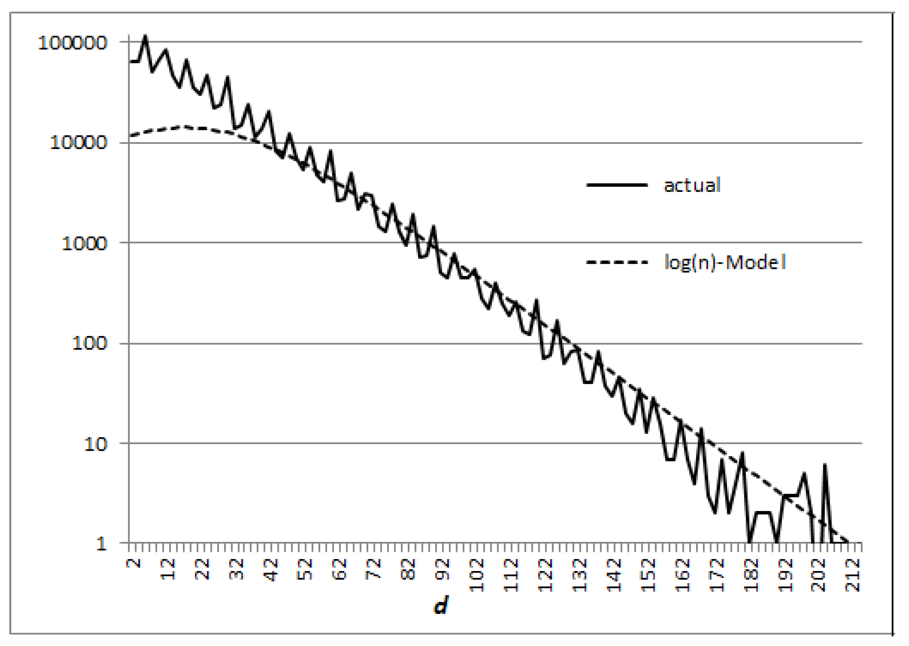
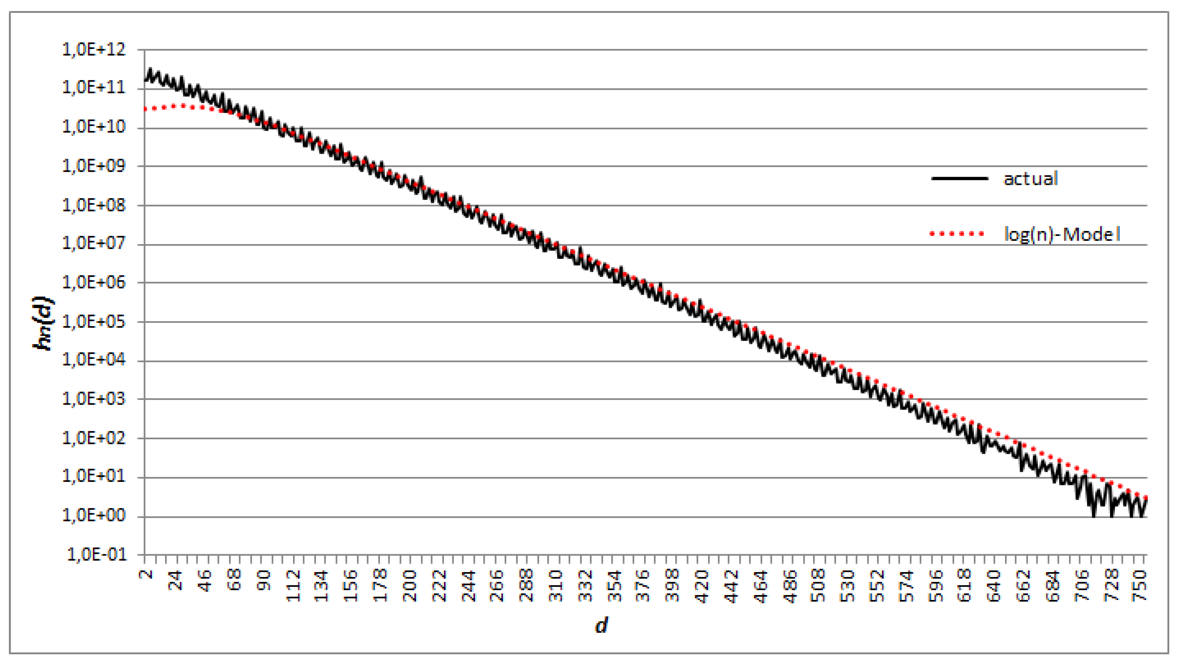
The general problem of prime pairs can be stated as follows: given d and N positive integers, d even, what is the number $H_N(d)$ of pairs of primes (not necessarily consecutive), $p,p^{\prime }\le N$ such that $p^{\prime }=p+d$? Connected with this there is the following one, we can call as the problem of counting successive prime pairs: given d and N positive integers, d even, what’s the number $h_N(d)$ of pairs of primes $p_i,p_{i+1}\le N$, separated by the gap d, that is such that $p_{i+1}=p_i+d$?

Mathematics has no certain results about these two problems which are different from the so called “bounded gaps problem”, recently solved by mathematician Yitang Zhang [36], who proved that as $i\to \infty$ there are infinitely many prime pairs $p_{i+1}-p_i=d$, with $d<7.0\times {10}^7$. Successively, this bound has been lowered to 246 through the extension of the method of Zhang and other contributors. Nevertheless, the twin primes conjecture which requires the bound to be reduced to $d=2$, remains unproven. Important results towards this goal can be found in [37,38], showing in particular that ${lim\; inf}_{i\to \infty }\frac{d}{ln{p}_i}=0$, that is there always be pairs of primes $p_{i+1}=p_i+d$ with d less than any fraction of $ln{p}_i$, the average spacing between successive primes.

In 1923, Hardy and Littlewood proposed the following formula as a solution of the general problem, stressing that it was impossible for them “to offer anything approaching a rigorous proof” (see Conjecture B, [5]):

$$H_N(d)\sim 2c_{2}J(d)\frac{N}{{ln}^{2}N}$$

(126)

where

$$c_2=\prod _{p>2}(1-\frac{1}{{(p-1)}^2})$$

(127)

$$J(d)=\prod _{p/d}\frac{p-1}{p-2}.$$

(128)

The product is over all odd primes in (127), over odd primes dividing d in (128). The constant $C_2=2c_2=1.32032363\cdots$ is called the twin prime constant, while the term $J(d)$ is responsible for the irregularities and the oscillating pattern of the counting functions. A formula similar to (126) for the counting of successive prime pairs separated by a gap d, was suggested by Wolf ([39], and the references therein) after enumerating, by means of a computer program, all gaps between consecutive primes up to $N=2^{44}\approx 1.76\times {10}^{13}$. Starting from the observed pattern, which showed an exponential decay of the number of pairs depending on d, at the end of a heuristic procedure including approximations due to PNT, he deduced the complete formula (the procedure is reported in M. Wolf (2018), Some Heuristics on the Gaps between Consecutive Primes, available at https://arxiv.org/abs/1102.0481 accessed on 31 March 2021).

$$h_N(d)\sim 2c_{2}J(d)\frac{{\pi }^2(N)}{N}{e}^{-d\pi (N)/N}.$$

(129)

The functional dependence on N of the formula above can be transformed into a dependence on the sequence number n of the greatest prime $p_n$ interested in the count. Indeed, we can set $N=p_n\sim nlnn$ and $\pi (N)=n$ and, hence, it is easy to get

$$\frac{{\pi }^2(N)}{N}{e}^{-d\pi (N)/N}\sim F_n(d)=\frac{n}{lnn}{e}^{-\frac{d}{lnn}}$$

(130)

and the counting formula becomes

$$h_n(d)\sim 2c_{2}J(d)\frac{n}{lnn}{e}^{-\frac{d}{lnn}}$$

(131)

where I changed the capital letter N to lower case n so as to remember the different meaning of the functional dependence.

The original Hardy and Littlewood conjecture was empirically tested by several authors and used to calculate the number of pairs $h_N(d)$ in the case of small gaps d between successive primes [40]. I show in the following that the conjecture of Wolf, which is based on a large amount of empirical data, can be derived from the combinatorial model we defined as log(n)-Model in Remark 19.

Remark 21.

Note that the conjecture (131) can be written as

$$h_n(d)\propto {\int }_1^n\frac{\partial F_t(d)}{\partial t}dt$$

where$F_n(d)$is the function defined in (130) and

$$\frac{\partial F_n(d)}{\partial n}=\frac{1}{lnn}{e}^{-\frac{d}{lnn}}(1+o(1)).$$

(132)

Definition 9.

Given the sequence of primes$\{p_n,n=1,2,3,\cdots \}$, let us define the gap$g_n$between successive primes and the number of successive prime pairs$h_n(d)$separated by a gap d depending on the sequence number n as

$$g_n=p_{n+1}-p_n$$

$$h_n(d)\#\{p_i:g_i=d,i\le n\}.$$

The gap $g_n$ can be modeled as the difference between the random variables

$$g_n=q_{n+1}-q_n$$

with probability mass function

$${\sigma }_n(d)={\int }_n^{\infty }{\varphi }_{n,n+1}(x,x+d)dx$$

(133)

where ${\varphi }_{n,n+1}(x,y)$ is the joint probability density function of the couple $(q_n,q_{n+1})$. We can obtain the estimate of the function $h_n(d)$, as resulting from the combinatorial model adopted, through the equation

$$h_n(d)=\sum _{i=1}^n{\sigma }_i(d)\approx {\int }_1^n{\sigma }_t(d)dt.$$

(134)

We do the following assumption.

Assumption 2.

(Large gaps independence law) For$d\gg 2$sufficiently large, the two events$q_n=x$and$q_{n+1}=x+d$are independent.

Under the previous assumption, the joint probability ${\varphi }_{n,n+1}(x,x+d)$ can be written as the product of the two probability density functions

$${\varphi }_{n,n+1}(x,x+d)={\varphi }_n(x){\varphi }_{n+1}(x+d),d\gg 1$$

(135)

and its value depends on the type of model we choose.

Let us calculate the joint probability (135) for the log(n)-Model defined in Remark 18.

We adopt the following approximations

$$ln(n+1)\approx lnn$$

and

$$r_{n+1}\approx r_n+lnn,n>1,$$

valid for both (this means the results we are going to obtain depend on PNT only, not on the Riemann Hypothesis).

$$r_n=nlnn$$

and

$$r_n=ali(n).$$

Then (135) becomes

$${\varphi }_n(x){\varphi }_{n+1}(x+d)=\frac{e{a}^2}{{ln}^{2}n}{e}^{-\frac{d}{lnn}}{e}^{-2(\frac{x-r_n}{lnn})}{e}^{-a{e}^{-(\frac{x-r_n}{lnn})}(1+e^{1-\frac{d}{lnn}})},$$

and (133), after the variable change

$$\frac{x-r_n}{lnn}=t,$$

is written

$${\sigma }_n(d)=\frac{e{a}^2}{lnn}{e}^{-\frac{d}{lnn}}{\int }_{\frac{n-r_n}{lnn}}^{\infty }{e}^{-2t}{e}^{-a{e}^{-t}(1+e^{1-\frac{d}{lnn}})}dt.$$

Let $\alpha$ be

$$\alpha =a(1+e^{1-\frac{d}{lnn}}),$$

then the integral

$${\int }_{\frac{n-r_n}{lnn}}^{\infty }{e}^{-2t}{e}^{-e^{-t}\alpha }dt=\frac{1}{{\alpha }^2}(1-e^{-\alpha e^{-\frac{n}{lnn}+n}}-\alpha e^{-\frac{n}{lnn}+n}{e}^{-\alpha e^{-\frac{n}{lnn}+n}})\approx \frac{1}{{\alpha }^2},\mathrm{for}n\gg 1.$$

Finally, the probability mass function (133) resulting from the log(n)-Model under Assumption 2 and $n\gg 1$ is (note it is independent of parameter a)

$${\sigma }_n(d)\approx \frac{e}{{(1+e^{1-\frac{d}{lnn}})}^2}\frac{e^{-\frac{d}{lnn}}}{lnn}.$$

(136)

Comparing the previous equation with (132), we see the log(n)-Model confirms Wolf’s conjecture, in particular the exponential decay of the pair number depending on d, at least for large values of the gap d, when Assumption 2 can be considered valid. Note that in the case of the n-Model, we would get the same expression as in (136), but with the function n in place of $lnn$. The fact that only the RH rule compliant model agrees with the counting function of consecutive prime pairs, derived from empirical data, is a notable achievement of the theory, since it is a strong indication that the counting problem is deeply connected with the Riemann Hypothesis.

Figure 1 and Figure 2 show the results obtained from the log(n)-Model with respect to the actual numbers of pairs in two cases: $49\times {10}^6<n\le 50\times {10}^6$ and $2^{47}\le p_n\le 2^{48}$.

Figure 1. Numbers of successive prime pairs as function of the gap $d=p_{n+1}-p_n$ in 49,000,000 $\le n\le$ 50,000,000 (logarithmic scale).

Figure 2. Numbers of successive prime pairs as function of the gap $d=p_{n+1}-p_n$ in 4,461,632,979,716 $\le n\le$ 8,731,188,863,469 (logarithmic scale).

5.3. A Heuristic Model of the Distribution of Prime Numbers

The generalized model we presented in Section 5.1 can be directly related to the sequence of primes by changing condition (115) into the following

$$E\left[q_n\right]=f(n)\left[ln({\lambda }_n)+\gamma \right]=p_n$$

(137)

which leads to the value

$${\lambda }_n=a{e}^{\frac{p_n}{f(n)}},\mathrm{with}a=e^{-\gamma }$$

while the point of maximum of the probability density function (113) becomes

$$x_M=p_n-\gamma f(n).$$

It is interesting to note we would obtain the same expressions, with $a=1$, if we substitute the condition (137) with the following one, on the point of maximum of the function ${\varphi }_n(x)$

$$x_M=f(n)ln({\lambda }_n)=p_n.$$

(138)

In this case, the mean value of $q_n$ changes to

$$E\left[q_n\right]=p_n+\gamma f(n).$$

This model has the property to express the prime counting function $\pi (k)$ through the values of the sequence of primes $p_n$ from $n=1$ to $n=k$. Let consider indeed the case when $f(n)=\sigma$ is constant. In this case, the average of the random counting variable (102) is

$$E\left[{\xi }_k\right]=\widehat{\pi }(k,\sigma )=\sum _{n=1}^k{e}^{-a{e}^{\frac{-k+p_n}{\sigma }}}$$

(139)

and it approximates the value of $\pi (k)$ with any precision depending on $\sigma$.

Remark 22.

It holds

$$\sum _{n=1}^{\pi (k)}{e}^{-a{e}^{\frac{-k+p_n}{\sigma }}}\le \widehat{\pi }(k,\sigma )\le \sum _{n=1}^{\pi (k)}{e}^{-a{e}^{\frac{-k+p_n}{\sigma }}}+1$$

(140)

for

$$\sigma <\frac{2}{lnln(k-\pi (k))+\gamma }$$

and

$$\underset{\sigma \to 0^{+}}{lim}\widehat{\pi }(k,\sigma )=\underset{\sigma \to 0^{+}}{lim}\sum _{n=1}^{\pi (k)}{e}^{-a{e}^{\frac{-k+p_n}{\sigma }}}=\pi (k).$$

(141)

Indeed

$$\widehat{\pi }(k,\sigma )=\sum _{n=1}^l{e}^{-a{e}^{\frac{-k+p_n}{\sigma }}}+\sum _{n=l+1}^k{e}^{-a{e}^{\frac{-k+p_n}{\sigma }}}$$

since

$$e^{-a{e}^{\frac{-k+p_{l+1}}{\sigma }}}>e^{-a{e}^{\frac{-k+p_n}{\sigma }}},n=l+2,\cdots ,k$$

we can write

$$\sum _{n=1}^l{e}^{-a{e}^{\frac{-k+p_n}{\sigma }}}\le \widehat{\pi }(k,\sigma )\le \sum _{n=1}^l{e}^{-a{e}^{\frac{-k+p_n}{\sigma }}}+e^{-a{e}^{\frac{-k+p_{l+1}}{\sigma }}}(k-l).$$

Assuming $l=\pi (k)$ and $e^{-a{e}^{\frac{-k+p_{l+1}}{\sigma }}}(k-l)\le 1$, (140) easily follows.

Note that for each term of the sum (139) it is

$$\underset{\sigma \to 0^{+}}{lim}{e}^{-a{e}^{\frac{-k+p_n}{\sigma }}}=\left\{\begin{array}{ccc}\hfill 1& ,& p_n<k\hfill \\ \hfill 0& ,& p_n>k\hfill \end{array}\right.$$

hence (141).

From Equation (137) we get in the case of the log(n)-Model, $f(n)=lnn$:

$${\varphi }_n(x)=\frac{a}{lnn}{e}^{-\frac{x-p_n}{lnn}}{e}^{-a{e}^{-\frac{x-p_n}{lnn}}},$$

(142)

$${\mathsf{\Phi }}_n(x)=e^{-a{e}^{-\frac{x-p_n}{lnn}}};$$

(143)

in the case of the n-Model, $f(n)=n$:

$${\varphi }_n(x)=\frac{a}{n}{e}^{-\frac{x-p_n}{n}}{e}^{-a{e}^{-\frac{x-p_n}{n}}},$$

(144)

$${\mathsf{\Phi }}_n(x)=e^{-a{e}^{-\frac{x-p_n}{n}}}.$$

(145)

The probability functions above are valid for $x\ge n$ (remember (110)), $n>1$ sufficiently large, and $a=e^{-\gamma }$.

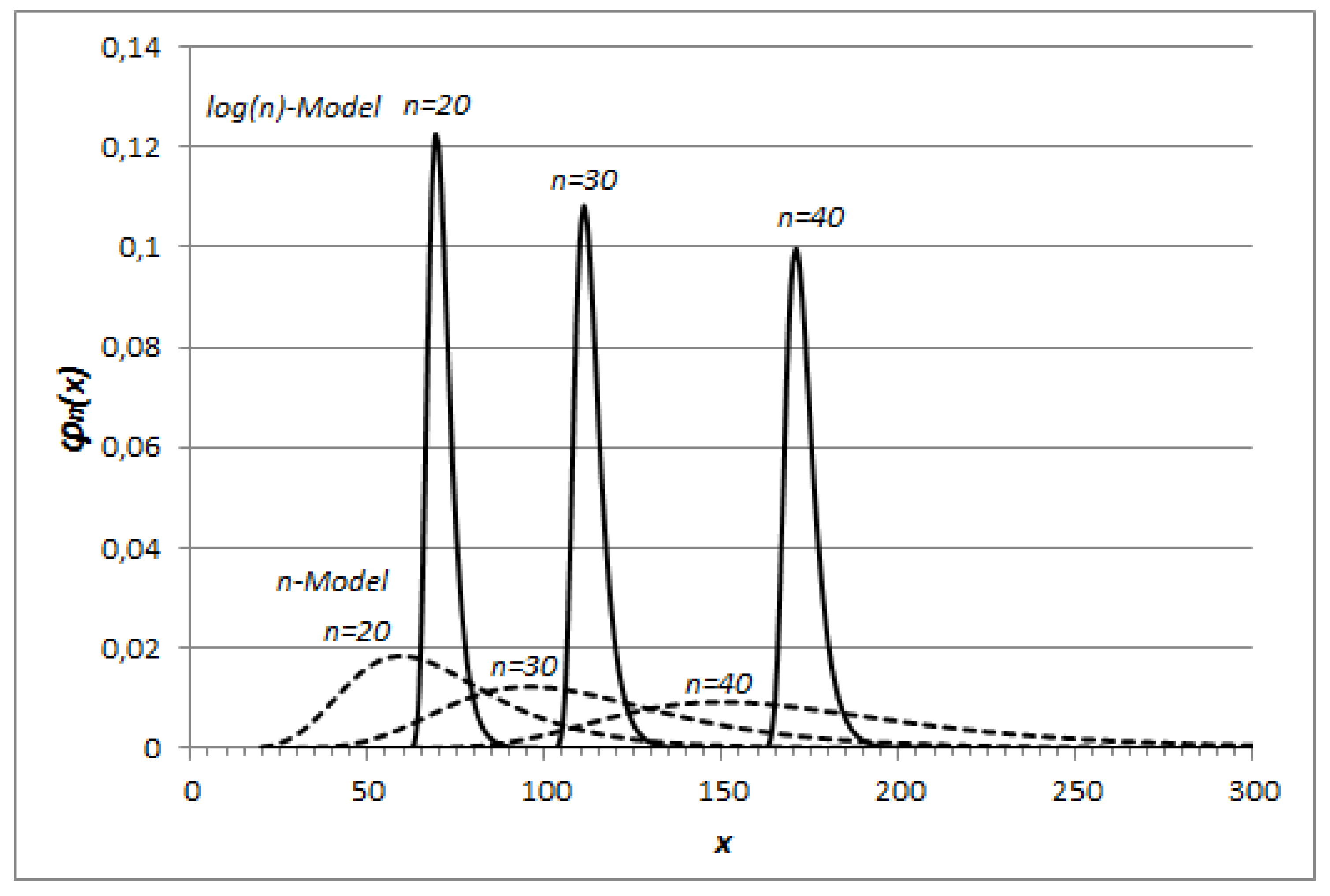
Definition 10.

Equations (142)–(145) define the heuristic log(n)-Model and the heuristic n-Model respectively.

Examples of different probability distribution functions ${\varphi }_n(x)$ resulting for these heuristic models are given in Figure 3, for $n=20,30,40$.

Figure 3. Heuristic model probability distribution functions ${\varphi }_n(x)$ for $n=20,30,40$.

From Figure 3, we see the dispersion of the random variable $q_n$ around its mean value $p_n$ is very small in the case of the heuristiclog(n)-Model, so that we can assume the estimate $\widehat{\pi }(k)$ is very close to the prime-counting function itself $\pi (k)$ for this model as stated by Remark 22 in the particular case $f(n)=constant$.

Table 5 shows some examples of estimate of $\pi (k)$, calculated through the heuristiclog(n)-Model with $a=e^{-\gamma }$, for different orders of magnitude.

Table 5. $\pi (k)$ estimate through heuristic log(n)-Model.

k	$\mathit{\pi }(\mathit{k})$	$\widehat{\mathit{\pi }}(\mathit{k})$
10	4	$4.33$
100	25	$25.50$
1000	168	$167.65$
10,000	1229	$1229.34$
100,000	9592	9592.09
1,000,000	78,498	78,498.23

The following considerations we propose in the case of the heuristic log(n)-Model, because of its relevance, are obviously valid in the case $f(n)=\sigma$, constant.

The following theorem gives a quantitative evaluation of the probability of error we do, when considering the random variable ${\xi }_k$ (in practice its mean value for small variances) as an estimate of $\pi (k)$.

Theorem 13.

Given the random variable${\xi }_k$of Definition 8,$ϵ>0$, let

$${\xi }_{p_n-\lceil ϵ\rceil }\ge n=\pi (p_n)$$

be the first kind error,

$${\xi }_{p_n+\lceil ϵ\rceil }<n=\pi (p_n)$$

the second kind error of${\xi }_k$at$k=p_n$and

$$W_{\xi }(n,ϵ)=Prob\{{\xi }_{p_n-\lceil ϵ\rceil }\ge n\}+Prob\{{\xi }_{p_n+\lceil ϵ\rceil }<n\}$$

the sum of the two error probabilities. Then for the heuristic log(n)-Model defined by Equations (142) and (143) with$a=e^{-\gamma }$it is

$$W_{\xi }(n,ϵ)\le \frac{{\pi }^2}{6}\frac{{ln}^{2}n}{{ϵ}^2}.$$

(146)

Proof. 

From the theory of Gumbel distribution we know the variance of $q_n$ is

$$E\left[{(q_n-p_n)}^2\right]=\frac{{\pi }^2}{6}{ln}^{2}n$$

hence from Chebyshev’s inequality

$$Prob\{|q_n-p_n|\ge ϵ\}\le \frac{{\pi }^2}{6}\frac{{ln}^{2}n}{{ϵ}^2}.$$

It is

$$Prob\{|q_n-p_n|\ge ϵ\}={\mathsf{\Phi }}_n(p_n-ϵ)+(1-{\mathsf{\Phi }}_n(p_n+ϵ))$$

and

$${\mathsf{\Phi }}_n(p_n-\lceil ϵ\rceil )+(1-{\mathsf{\Phi }}_n(p_n+\lceil ϵ\rceil ))<{\mathsf{\Phi }}_n(p_n-ϵ)+(1-{\mathsf{\Phi }}_n(p_n+ϵ)),$$

and, therefore, we can also write

$${\mathsf{\Phi }}_n(p_n-\lceil ϵ\rceil )+(1-{\mathsf{\Phi }}_n(p_n+\lceil ϵ\rceil ))\le \frac{{\pi }^2}{6}\frac{{ln}^{2}n}{{ϵ}^2}.$$

From (99), (100) it follows

$${\mathsf{\Phi }}_n(p_n-\lceil ϵ\rceil )=Prob\{{\xi }_{p_n-\lceil ϵ\rceil }\ge n\}$$

$$(1-{\mathsf{\Phi }}_n(p_n+\lceil ϵ\rceil ))=1-Prob\{{\xi }_{p_n+\lceil ϵ\rceil }\ge n\}=Prob\{{\xi }_{p_n+\lceil ϵ\rceil }<n\}$$

$$Prob\{{\xi }_{p_n-\lceil ϵ\rceil }\ge n\}+Prob\{{\xi }_{p_n+\lceil ϵ\rceil }<n\}\le \frac{{\pi }^2}{6}\frac{{ln}^{2}n}{{ϵ}^2}.$$

□

Remark 23.

Through the heuristic model we can derive new lower and upper bounds of the prime-counting function$\pi (k)$:

$${\int }_1^k{e}^{-a{e}^{\frac{-k+\beta (n)}{lnn}}}dn\le \pi (k)\le {\int }_1^k{e}^{-a{e}^{\frac{-k+\alpha (n)}{lnn}}}dn,$$

(147)

where

$$\alpha (n)=n(lnn+lnlnn-1),$$

(148)

$$\beta (n)=n(lnn+lnlnn).$$

(149)

We know ([41,42]) the following lower and upper bounds of the n-th prime $p_n$ hold

$$\alpha (n)<p_n<\beta (n)$$

for $n\ge 2$ the left-hand side and $n\ge 6$ the right-hand side, hence for ${\mathsf{\Phi }}_n(k)$ given by (143) it follows

$$e^{-a{e}^{\frac{-k+\beta (n)}{lnn}}}\le {\mathsf{\Phi }}_n(k)\le e^{-a{e}^{\frac{-k+\alpha (n)}{lnn}}},n\ge 6,$$

(150)

and assuming $k\gg 6$ sufficiently large so that the condition $n\ge 6$ may be neglected, we can write (147) for $\widehat{\pi }(k)$ given by

$$\widehat{\pi }(k)=\sum _{n=1}^k{\mathsf{\Phi }}_n(k).$$

From Remark 22 and Theorem 13, we know we can consider the approximation $\widehat{\pi }(k)\approx \pi (k)$ as valid for the heuristic model, from which we get (147).

6. Concluding Remarks

The first aim of this work was to deepen the problem of randomness in the distribution of prime numbers through such simple combinatorial objects as First Occurrence Sequences, showing new analogies between the classical set partition problem and the distribution of primes themselves. First Occurrence Sequences define a general class of objects for which the Prime Number Theorem holds, such as for the prime sequence, but they fail to represent more stringent constraints, required by the Riemann Hypothesis, such as the equivalent condition established by Helge von Koch I called RH rule. In order to investigate this second step, the simple model must be generalized (or the class of combinatorial objects must be restricted) to discriminate between RH rule compliant and noncompliant models. The analysis based on probability methods shows the Riemann Hypothesis holds w.p. 1 (together with the Prime Number Theorem, of course) for the class of random sequences represented by the log(n)-Model with mean equal to $ali(n)$, the inverse function of the logarithmic integral function. Therefore, we can conclude that the property represented by the Riemann Hypothesis through the RH rule is largely independent of the primes and belongs to a large class of random sequences. Whether this class also contains the sequence of prime numbers cannot be decided by the model except statistically. Something similar happens within the context of analytical theory when speaking of zeta function $\zeta (s)$, Dirichlet L-functions $L(s,\chi )$ (Chap. 12, [43]) (s is the complex variable $s=\sigma +it$), and the Generalized Riemann Hypothesis “that is the hypothesis that not only $\zeta (s)$ but all the functions $L(s,\chi )$ have their zeros in the critical strip on the line $\sigma =\frac{1}{2}$” (p. 124, [44]).

Attempts to prove the Riemann hypothesis through the methods of physics go back as far as the so-called Hilbert–Polya conjecture, which associates the imaginary part of non-trivial zeros of $\zeta (s)$ to the eigenvalues of some self-adjoint (Hermitian) operator that might be considered like the Hamiltonian of a physical system (the story of Hilbert–Polya conjecture is documented on Odlyzko’s personal website; see http://www.dtc.umn.edu/~odlyzko/ accessed on 31 March 2021). Each type of combinatorial model we presented in the previous sections, based on probability equations such as (111) and more generally (25), can be transformed into a single particle Hamiltonian of an equivalent quantum system that emerges as a solution to an underlying combinatorial problem. This topic is outside the scope of this work and will not be treated here; I just want to mention that the analogy with the physical problem allows us to overcome some critical points of the combinatorial model and eliminate any arbitrariness in the choice of the mean of the random variable $q_n$ (the combinatorial counterpart of the n-th prime). The solution $ali(n)$ emerges as a general asymptotic solution for such models due to concepts such as interaction potential and energy levels, that play an important role also in describing integer sequences such as Fibonacci numbers and prime numbers, and the application of the Hellmann–Feynman theorem to the whole system (see [45] for a mathematical foundation of the theorem). These methods result in computational benefits improving the estimates obtained from the combinatorial model and may suggest new conjectures about the distribution of primes. In [29], the quantum model derived from what we have called n-Model is developed and applied to explore the region beyond the Skewes number in connection with the numerical results known in the literature derived through analytical methods.

These two topics (the parallelism between the treatment from the point of view of random sequences and of Riemann zeta and Dirichlet L-functions; the transposition of the problem into a quantum physics framework), seem worthy of being addressed in future work.