Article

The Novel Integral Homotopy Expansive Method

by
Uriel Filobello-Nino
1,
Hector Vazquez-Leal
1,2,*,
Jesus Huerta-Chua
3,
Jaime Ramirez-Angulo
3,
Darwin Mayorga-Cruz
2,4 and
Rogelio Alejandro Callejas-Molina
5
1
Facultad de Instrumentación Electrónica, Universidad Veracruzana, Cto. Gonzalo Aguirre Beltrán S/N, Xalapa 91000, Mexico
2
Consejo Veracruzano de Investigación Científica y Desarrollo Tecnológico (COVEICYDET), Av Rafael Murillo Vidal No. 1735, Cuauhtémoc, Xalapa 91069, Mexico
3
Instituto Tecnológico Superior de Poza Rica, Tecnológico Nacional de México, Luis Donaldo Colosio Murrieta S/N, Arroyo del Maíz, Poza Rica 93230, Mexico
4
Centro de Investigación en Ingeniería y Ciencias Aplicadas, CIICAP, Universidad Autónoma del Estado de Morelos, Cuernavaca 62209, Mexico
5
Instituto Tecnológico de Celaya, Tecnológico Nacional de México, Antonio García Cubas Pte. 600, Celaya 38010, Mexico
*
Author to whom correspondence should be addressed.
Mathematics 2021, 9(11), 1204; https://doi.org/10.3390/math9111204
Submission received: 21 April 2021 / Revised: 16 May 2021 / Accepted: 21 May 2021 / Published: 26 May 2021

Abstract

:
This work proposes the Integral Homotopy Expansive Method (IHEM) in order to find both analytical approximate and exact solutions for linear and nonlinear differential equations. The proposal consists of providing a versatile method able to provide analytical expressions that adequately describe the scientific phenomena considered. In this analysis, it is observed that the proposed solutions are compact and easy to evaluate, which is ideal for practical applications. The method expresses a differential equation as an integral equation and expresses the integrand of the equation in terms of a homotopy. As a matter of fact, IHEM will take advantage of the homotopy flexibility in order to introduce adjusting parameters and convenient functions with the purpose of acquiring better results. In a sequence, another advantage of IHEM is the chance to distribute one or more of the initial conditions in the different iterations of the proposed method. This scheme is employed in order to introduce some additional adjusting parameters with the purpose of acquiring accurate analytical approximate solutions.

1. Introduction

Modeling natural processes in the mathematical realm is certainly a complex task. Most of these processes are nonlinear; thus, there is a need to use complicated mathematical calculations to acquire an approximate value, which is not always the desired result. The use of differential equations has proven to be useful in order to find meaningful results.
Natural processes give rise to scientific problems and to the proposal of new methods in order to reach exact and approximate solutions to the differential equations that govern said nonlinear problems; however, the search for such solutions is not an easy task and justifies all the research efforts carried out on this topic. As is well known, solving linear differential equations is a field dominated by certain ideas—in particular, by the theory of ordinary differential equations (ODES), which provides exact solutions and the methods of finding solutions are found in texts of differential equations [1]. Unlike linear ODES, in the case of nonlinear differential equations, an exact solution to a given nonlinear problem can rarely be obtained [2], although this work will show the potentiality of the proposed method finding both exact and approximate solutions. The diversity of nonlinear problems has led to the proposal of several methods as alternatives to classical methods, with the aim to produce various types of nonlinear differential equations. Numerical methods are a part of the analysis that provide algorithms to acquire approximations of differential equations. Unlike symbolic computation, numerical methods handle numbers [3,4,5]. On the other hand, the use of analytical methods in order to acquire exact and analytical approximate solutions to solve nonlinear ordinary differential equations is well known. Next, we provide a list with some of the most employed methods in accordance with the literature: variational approaches [6,7,8], the tanh method [9], the exp-function [10,11], Adomian’s decomposition method [12,13,14,15,16,17], parameter expansion [18], the homotopy perturbation method (HPM) [8,17,19,20,21,22,23,24,25,26,27,28,29,30,31,32,33,34], perturbation method [35,36,37,38], modified Taylor series method [39], Picard method [40], PSEM method [41,42,43,44], Homotopy Analysis Method [45,46,47,48], the variational iteration method [49], the Hirota bilinear formulation [50,51,52], the continuum-cancelation Leal method [53], Leal Polynomials [54], among many others.
This work introduces the Novel Integral Homotopy Expansive Method (IHEM), which as we will see employs the concept of homotopy. In the same way, we will show that the IHEM method is relatively easy to use and provides both exact and approximate solutions. Another useful method based on the concept of homotopy is the Homotopy Analysis Method (HAM), which has been employed to solve nonlinear differential equations and integral equations in science and engineering [45,46,47,48]. Unlike the proposed method, HAM is a nonperturbative analytical method that offers the possibility to adjust and control the convergence of its solutions by using the so-called convergence control parameter. On the other hand, the IHEM method starts expressing a differential equation as an integral equation. We will see that in order to guarantee the accuracy of the obtained solutions, IHEM provides the possibility of adequately adjusting certain parameters of the method with the aim to increase the precision of the obtained solutions. IHEM proposes at least two possibilities: the first is based on the Least Square Method LSM [55], which is a well established method. The second possibility calculates the above mentioned parameters using the numerical solution of the problem to solve. Next, we will summarize the IHEM method as follows. Given an ordinary differential equation, the method expresses it as an integral equation, for which it solves for the y somehow. In this point we express the integrand of the equation in terms of an homotopy and assume that the incognita function y is expressed as a power series of homotopy parameter p [24,26] in such a way that after equating identical powers of p terms, in both sides of the integral equation there can be found values for a sequence of unknown functions which determine the IHEM solution. The precision of the obtained results will show the potentiality of the proposed method for applications.
The rest of this work is as follows. Section 2 introduces the formulation of the IHEM method. Additionally, Section 3 presents the application of the proposed method, in the search for exact and approximate solutions for some relevant scientific problems. Section 4 offers a whole discussion about the proposed solutions for three case studies as well as the advantages of using IHEM. Finally, a brief conclusion of the relevant aspects of this work is given in Section 5.

2. IHEM Method

To understand how IHEM works, consider a general nonlinear differential equation, which can be expressed as follows [24,26]
L ( u ) + N ( u ) f ( r ) = 0 . r Ω ,
with the following boundary conditions
B ( u , u / n ) = 0 , r Γ .
Above, B symbolizes a boundary operator, f ( r ) is a given analytical function and Γ is the domain boundary for Ω , while L and N are, respectively, linear and nonlinear operators.
In accordance with the proposed method, from (1) we solve for u in terms of the following integral equation:
u ( r ) = a + b r + r 0 r r 0 r ( f ( r ) N ( u ( r ) ) ) d r d r ,
where we have supposed that L is a second order linear operator. Of course, there exist many different ways to solve for u ( r ) .
Next, we introduced a homotopy into the integral (3) and at the same time we assume that incognita function u is expressed as a power series of homotopy parameter p
u ( r ) = v 0 ( r ) + v 1 ( r ) p + v 2 ( r ) p 2 +
so that we get
n = 0 p n ν n = a + b r + r 0 r r 0 r ( 1 p ) w ( r ) + p f ( r ) N n = 0 p n ν n d r d r ,
where p is the homotopy parameter, whose values belong to the interval [ 0 , 1 ] and w ( r ) is a function that is introduced that takes advantage of the flexibility of the homotopy technique (it is frequently introduced as an adjusting parameter K).
Next, equating identical powers of p terms, there can be found values for the sequence ν o , ν 1 , ν 2 , after solving in a systematic way the integrals that emerge from the different orders.
ν 0 = a + b r + r 0 r r 0 r w ( r ) d r d r , ν 1 = r 0 r r 0 r ( w ( r ) + f ( r ) N ν 0 d r d r , ν 2 = r 0 r r 0 r N ν 0 , ν 1 d r d r , ν 3 = r 0 r r 0 r N ν 0 , ν 1 , ν 2 d r d r , ν j = r 0 r r 0 r N ν 0 , ν 1 , ν 2 , ν 3 , , ν j 1 d r d r
Thus, in order to acquire an approximate or exact solution for (1), we substituted the results from (6) into (4), taking the limit p 1 , which led to a solution as follows [24,26].
U ( x ) = v 0 ( x ) + v 1 ( x ) + v 2 ( x ) + v 3 ( x ) . . .
Another advantage of IHEM is the chance to easily distribute one or more of the initial conditions in the different iterations of the proposed method. This is employed in order to introduce adjusting parameters with the purpose to obtain a better solution for (1).
In this case, (5) would assume the form:
n = 0 p n ν n = A 0 + A 1 p + A 2 p 2 + + b r + r 0 r r 0 r ( 1 p ) w ( r ) + p f ( r ) N n = 0 p n ν n d r d r ,
assuming that we propose to distribute the initial conditions and of course fulfilled the limit
lim p 1 A 0 + A 1 p + A 2 p 2 + . . .   = a .
Although Equation (1) is in principle general, it is possible to provide nonlinear examples from the physical point of view. For the common case of a second order linear operator, the equation of motion for an undamped pendulum of length l, whose bob has mass m, is given by
d 2 x d t 2 + g l sin x = 0 ;
where x is the angle of deviation. In this case,
L = d 2 x d t 2 , N = g l sin x , f = 0 .
For the case where exist a damping force proportional to the velocity of the bob, then
d 2 x d t 2 + c m d x d t + g l sin x = 0 ;
in this equation
L = d 2 x d t 2 + c m d x d t , N = g l sin x , f = 0 .
In the theory of the vacuum tube, the Van der Pool equation is given by
d 2 x d t 2 + μ ( x 2 1 ) d x d t + x = 0 ;
where
L = d 2 x d t 2 μ d x d t + x , N = μ x 2 d x d t , f = 0 .
Other important particular case of the Equation (1) is the damped and driven Duffing equation, which is expressed as
d 2 x d t 2 + A d x d t + B x + C x 3 = D cos ( w t ) ,
in this equation
L = d 2 x d t 2 + A d x d t + B x , N = C x 3 , f = D cos ( w t ) .

3. Case Studies

This section will study three case studies in order to show the potentiality of IHEM.

3.1. Case Study 1

Next, we will find an analytical approximate solution for the second order nonlinear differential equation:
y ( x ) + ε ( y ( x ) y ( x ) + y 2 ( x ) ) = 0 ,
y ( 0 ) = 1 , y ( 1 ) = 0 , 0 x 1 .
This equation describes the steady state one-dimensional conduction of heat in an insulated slab with the thermal conductivity linearly dependent on the temperature. In this equation, y ( x ) is a dimensionless quantity that depends, in a proportional way, on the temperature y = T T 2 T 1 T 2 , where T is the temperature of the system and T 1 and T 2 are the fixed temperatures of the two opposite faces of the slab where it is assumed that T 2 < T 1 , x is a dimensionless quantity proportional at the distance measured from the front of the slab, and inversely proportional to the total length of the slab, while parameter ε is proportional to the difference of temperatures of the two opposite faces of the slab [20,55]; as a matter of fact, this example considers a value of one for this parameter.
First, we express (10) as an integral equation as follows
y ( x ) = 1 + α x 0 x 0 x ( y y + y 2 ) d x d x ,
In accordance with (5), we obtained the following homotopy equation from (12)
n = 0 p n y n = 1 + α x 0 x 0 x ( 1 p ) w ( x ) + p n = 0 p n y n m = 0 p m y m + s = 0 p s y s 2 d x d x .
This first case study proposes to obtain a solution without using the possible advantage of the additional function w ( x ) ; therefore, by choosing w ( x ) = 0 , Equation (13) is reduced to
n = 0 p n y n = 1 + α x 0 x 0 x p n = 0 p n y n m = 0 p m y m + s = 0 p s y s 2 d x d x .
After equating identical powers of p terms, there can be found the following integrals that emerge from the different orders
y 0 ( x ) = 1 + α x ,
y 1 ( x ) = 0 x 0 x ( α 2 ) d x d x ,
y 2 ( x ) = 0 x 0 x ( y 0 y 1 + y 1 y 0 + 2 y 0 y 1 ) d x d x ,
y 3 ( x ) = 0 x 0 x ( y 0 y 2 + y 1 y 1 + y 2 y 0 + 2 y 0 y 2 + y 1 2 ) d x d x ,
After resolving recursively the integrals (15)–(18), we obtained the following results:
y 0 ( x ) = 1 + α x ,
y 1 ( x ) = α 2 x 2 2 ,
y 2 ( x ) = α 2 x 2 2 + α 3 x 3 2 ,
y 3 ( x ) = α 2 x 2 2 α 3 x 3 5 α 4 x 4 8 ,
Assuming that the third order approximation is sufficient, and after substituting the results of Equations (19) and (20)–(22) into (7), we obtained the following simple fourth order polynomial.
y ( x ) = 1 + α x α 2 x 2 2 α 3 x 3 2 5 α 4 x 4 8 .
In order to determine the value of the parameter, we followed the expected way to obtain an equation for the condition y ( 1 ) = 0 , applied to (23):
1 + α α 2 2 α 3 2 5 α 4 8 = 0 .
The solution for (24) is given by
α = 0.740722 .
After substituting (25) into (23), we obtained the following approximation for the proposed problem:
y ( x ) = 1 0.740722 x 0.274334 x 2 + 0.203205 x 3 0.188148 x 4 .
Essentially, IHEM expressed the nonlinear problems (10) and (11) in terms of the solution of the algebraic Equation (24) for this case.
Although (26) was obtained only to exemplify the method without the objective of achieving precision, the following table of values for the relative error, committed by using (26), shows that the above polynomial has good accuracy. With the exception of x = 0.9 , all the obtained y-values report relative errors between 0.0392 % and 1.11 % . On the other hand, in order to compare (26) with some approximation of the literature, Table 1 shows the comparison between the IHEM solution (26) with the corresponding solution obtained by the Modified Homotopy Perturbation Method coupled with Laplace Transform (MHPMLT) [20] for the same problem. We noted that both are precise, although (26) is better. Additionally, IHEM is easier to use as it is based on elementary integrals, unlike the MHPMLT method, which requires commanding the Laplace transform and its properties, making the MHPMLT algorithm complicated to implement.

3.2. Case Study 2

We will employ IHEM in order to calculate exact solutions for two second order nonlinear differential equations:
y ( x ) + 2 x y ( x ) + y n ( x ) = 0 ,
y ( 0 ) = 1 , y ( 0 ) = 0 ,
where n represents the called index of (27).
Equation (27) is denominated the Lane–Emden singular equation, its importance lies in that it is related to a great deal of phenomena in physics, such as stellar structure, thermal history of spherical cloud of gas, and thermionic currents, among others.
For the case of application of (27) to stellar structure, y ( x ) is a variable related to the density of a star [20,56] and x is a quantity proportional at the distance measured from the center of the star. The values of n are relevant to the following cases: the value n = 0 , corresponds to the case where the density as a function of the radius is constant, n = 1 adequately approximates a fully convective star and n = 3 corresponds to a fully radiative star, which represents a useful approximation for the sun. Other important results for Lane–Emden equation emerge from the fact that it possesses an exact solution for the cases: n = 0 , n = 1 and n = 5 . We employed IHEM in order to calculate exact solutions for the cases n = 0 and n = 1 , with the solutions:
n = 0 , y ( x ) = 1 x 2 6 ; n = 1 , y ( x ) = sin x x .
First, we will express (27) in terms of an integral equation from the first two terms.
Let it be the substitution:
U = y ,
then, (27) can be expressed as
U ( x ) + 2 x U = y n ( x ) .
After multiplying (31) for the integrating factor:
μ = e 2 x d x = x 2 ,
d ( U x 2 ) d x = x 2 y n ( x ) .
or
U = c x 2 x 2 0 x x 2 y n d x .
After using (30), it is possible to rewrite (34) as follows
y ( x ) = d c x 1 0 x x 2 0 x x 2 y n d x d x ,
from the first initial condition of (28), (35) is expressed as
y ( x ) = 1 0 x x 2 0 x x 2 y n d x d x .
For the case n = 1, (36) is reduced to
y ( x ) = 1 0 x x 2 0 x x 2 y d x d x .
Next, we introduced the following homotopy in accordance with IHEM:
n = 0 p n y n = 1 0 x x 2 0 x ( 1 p ) x 2 + p x 2 n = 0 p n y n d x d x ,
after we have chosen w ( x ) = x 2 (see (5)).
After equating identical powers of p terms, the following integrals can be found.
y 0 ( x ) = 1 0 x x 2 0 x x 2 d x d x ,
y 1 ( x ) = x 2 x 2 + x 2 y 0 d x d x ,
y 2 ( x ) = 0 x x 2 0 x x 2 y 1 d x d x ,
y 3 ( x ) = 0 x x 2 0 x x 2 y 2 d x d x ,
After recursively resolving the above integrals (39)–(42), we obtained the following results:
y 0 ( x ) = 1 x 2 6 ,
y 1 ( x ) = x 4 120 ,
y 2 ( x ) = x 6 5040 ,
y 3 ( x ) = x 8 362880 ,
Maintaining the third order approximation, and then substituting Equations (43)–(46) into (7), we obtain
y ( x ) = 1 x 2 6 + x 4 120 x 6 5040 + x 8 362880
From the Taylor series for s i n ( x ) , we rewrite (47) as:
y ( x ) = sin x x ,
see (29).
IHEM provides an exact solution. We note that a function is defined in the more general form through its power series; as a matter of fact, in this case it is complicated to obtain (48) in a different way.
With the aim to compare the performance of IHEM, next we provide the solution obtained from the third order standard HPM [24,26] for the same problem by using the initial function y 0 ( x ) = 1 , which is the first approximation for the solution of (27) ( n = 1 ), which satisfies the initial conditions.
y ( x ) = 1 3 x 2 2 5 x 4 72 x 6 720 +
From the comparison of (47) (the correct series) and (49), it is clear that third order standard HPM solution is not close to the right solution as, when comparing identical powers of x, the coefficients are totally different; therefore, the convergence of HPM approximation is slow, or (49) is a bad approximation considering that HPM was unable to adequately handle the singular point x = 0 .
For the case n = 0, (36) is expressed as
y ( x ) = 1 0 x x 2 0 x x 2 d x d x .
Although (50) is integrable, it is still possible to propose a homotopy in accordance with IHEM.
n = 0 p n y n = 1 0 x x 2 0 x ( 1 p ) x 2 + p x 2 d x d x ,
y 0 ( x ) = 1 0 x x 2 0 x x 2 d x d x ,
and for the other orders.
y 1 ( x ) = y 2 ( x ) = y 3 ( x ) = . . . = 0 .
After integrating (52) (or (50)), we obtained
y 0 ( x ) = 1 x 2 6 ,
essentially, Equation (54) is the exact solution for the proposed problem.

3.3. Case Study 3

We employed IHEM with the purpose to find an analytical approximate solution for the first order nonlinear differential equation:
y ( x ) + ε y ( x ) y ( x ) + y ( x ) = 0 ,
y ( 0 ) = 1 , x [ 0 , ) .
Equation (55) with initial condition (56) describes the important problem of cooling of a lumped system, volume V, surface area A, density ρ , and a variable specific heat c, which depends linearly of temperature and exposed to a convective environment at a fixed temperature T a [38,55]. In a sequence, y ( x ) is a dimensionless quantity that is expressed as a linear function of the temperature of the system y = T T a T i T a , where T is the temperature of the system and T i is its initial temperature ( T a < T i ), x is a variable that is directly proportional to time, and the parameter ε is an important quantity, directly related to the difference between the system’s initial temperature and the fixed environment’s temperature T a [38,55].
We expressed the problems (55) and (56), defined originally in a semi-infinite interval, in an equivalent problem defined in the finite interval [ 0 , 1 ] . Then, IHEM was used with the purpose to find an analytical approximate solution for the proposed problem.
To achieve this goal, let
X = 1 e x ,
We note that when x = 0 , then X = 0 , and x = implies X = 1 .
By using the chain rule, the following transformation between derivatives is clear:
y ( x ) = ( 1 X ) y ( X ) .
Therefore, substituting (58) into (55), we obtained the equivalent system.
y ( X ) ( 1 X ) + ε y ( X ) y ( X ) ( 1 X ) + y ( X ) = 0 ,
y ( 0 ) = 1 , X [ 0 , 1 ] .
Next, (59) is rewritten as the integral equation:
y ( X ) = 1 + 0 X X y ( X ) ε y ( X ) y ( X ) ( 1 X ) y ( X ) d X .
We solved (59) and (60), using the form (8), distributing the initial condition in the different iterations with the aim to obtain adjusting parameters.
Thus, in accordance with (8), we expressed (61) in terms of the following homotopy.
n = 0 p n ν n = A 0 + A 1 p + A 2 p 2 + + 0 X ( 1 p ) D + p X n = 0 p n ν n ε n = 0 p n ν n m = 0 p m ν m 1 X n = 0 p n ν n d X .
where D is a unknown parameter introduced taking advantage of the flexibility of the proposed method and it will be determined later.
As usual, after equating identical powers of p terms, we obtained:
y 0 ( X ) = A 0 + 0 X D d X ,
y 1 ( X ) = A 1 + 0 X D + X y 0 ε y 0 y 0 + ε X y 0 y 0 y 0 d X ,
y 2 = 0 X X y 1 ε y 0 y 1 + y 1 y 0 + ε X y 0 y 1 + y 1 y 0 y 1 d X ,
After resolving the above integrals, we obtained the following results:
y 0 ( X ) = A + D X ,
y 1 ( X ) = A 1 A 0 + D + ε A 0 D X ε D 2 2 ε A 0 D 2 X 2 + ε D 2 3 X 3 ,
y 2 ( X ) = A 2 + A 1 + ε A 0 k 1 ε A 1 D X + ε D k 1 + ε A 1 D 2 + ε A 0 k 2 ε A 0 k 1 2 X 2 + k 2 3 + ε D k 2 ε 2 D 3 3 ε 2 D 2 A 0 3 2 3 ε D k 1 2 ε A 0 k 2 3 X 3 + ε D 2 6 ε 2 D 3 4 3 ε D k 2 4 + ε 2 D 2 A 0 4 X 4 + 4 15 ε 2 D 3 X 5 ,
where:
k 1 = A 0 + D + ε A 0 D ; k 2 = ε D 2 2 ε A 0 D 2 .
By substituting (66)–(68) into (7), we obtained an analytical approximate solution:
y ( X ) = n = 0 2 y n ( X ) ,
where from (9) we employed the limit value:
lim p 1 A 0 + A 1 p + A 2 p 2 +   = 1 .
With the purpose to show the pertinence of IHEM solution (70), we calculated the unknown quantities A 0 , A 1 , and D by using the numeric solution with the aim to provide three points for the case ε = 0.5 (see Discussion section for another possibility).
( 0.25 , 0.8204473 ) , ( 0.75 , 0.3465973 ) , and ( 1 , 0 ) .
After substituting (72) into (70), we obtained an algebraic system of three equations with the three unknown quantities A 0 , A 1 , and D.
The solution of this system is given by
A 0 = 0.6140207 , A 1 = 0.8189641 , D = 2.0087588 .
The substitution of (73) into (70) yields a fifth order polynomial.
y ( X ) = 1 0.64964702 X 0.409364053 X 2 + 0.836007110 X 3 1.317367186 X 4 + 0.540371149 X 5 .
This approximation is defined in the interval [ 0 , 1 ] . On the other hand, the direct substitution of (57) into (74) results in an approximate solution for the original problems (55) and (56), but for the interval x [ 0 , ) .
y ( x ) = 1 0.64964702 ( 1 e x ) 0.409364053 ( 1 e x ) 2 + 0.836007110 ( 1 e x ) 3 1.317367186 ( 1 e x ) 4 + 0.540371149 ( 1 e x ) 5 ,
Figure 1 and Figure 2 show the precision of (74) and (75) (see Discussion).

4. Discussion

Next, we will present the main results obtained for this work. In particular we will emphasize the advantages of applying IHEM in order to obtain exact or approximate solutions both for nonlinear and linear differential equations. Such as we showed in this work, the IHEM algorithm possesses versatility in order to face different difficulties arising from the diversity of ODES. As a matter of fact, the case studies proposed for IHEM were chosen not only for their scientific interest, but in order to expose the performance of the proposed method in various situations.
In general terms, Section 2 exposed the fundaments of IHEM. One advantage of the method in relation to other iterative methods (for example, HPM [24,26]) is that due to the way IHEM presents the different iterations, it requires only integrations that are, most of the time, elementary, which occurred with the discussed case studies, while methods such as HPM and PM have to solve a set of coupled differential equations for each iteration.
Given the flexibility of the homotopy technique, the method allows to introduce adjusting parameters or even functions, with the purpose to improve the results of the proposed method. In formulations (5) and (8), we note the presence of a function w ( x ) , which turns out to be of paramount importance, as was exhibited in the solved examples. On the other hand, (8) showed the ease with which the initial conditions of a given problem can be distributed in the different iterations of the proposed IHEM method. This was employed in order to introduce adjusting parameters with the purpose to obtain a better solution for a differential equation.
Next, we provide a brief explanation about the relevant role played by the IHEM method in the solution of the proposed problems. Case study 1 is a relevant problem that describes the steady state one-dimensional conduction of heat in an insulated slab, with thermal conductivity linearly dependent on the temperature. We expressed this problem in terms of the homotopy Equation ((5)) and selected the function w ( x ) = 0 that is, without using the possible advantage of the additional function w ( x ) ; therefore, we kept only one unknown quantity to determine—the initial value of the derivative. With the aim to determine the value of the above mentioned parameter, we followed the common method to obtain an equation for the unknown from the condition y ( 1 ) = 0 . In addition to the handiness of the proposed solution (26), Table 1 for the relative error committed shows that it has good accuracy. We emphasize the ease with which this result can be obtained.
In order to compare (26) with some approximation from the literature, Table 1 showed the comparison between IHEM (26) and MHPMLT [20] for the same problem. In addition to (26) being better, IHEM is easier to use as it is based on elementary integrals, unlike MHPMLT, which needs to command the Laplace transform, its properties, as well as the MHPMLT algorithm.
From Table 1, we note that the proposed approximate solution (26) monotonically decreased from 1 to 0; this behaviour is physically expected as the distribution of temperatures under steady conditions does not depend explicitly on time and we assumed that T 2 < T 1 , where T 1 and T 2 are the fixed temperatures of the two opposite faces of the slab. The temperature along the slab has to be independent of the time and varies continuously from 1 to 0. The reliability of the results obtained for (26) was deduced from the same table, where we found that (26) has good precision.
Case 2 is concerned with the denominated Lane–Emden singular equation; its importance lies in the fact that it is related to a great deal of phenomena in physics, such as stellar structure, thermal history of spherical clouds of gas, and thermionic currents, among others. We employed IHEM in order to calculate exact solutions for the values n = 0 , and n = 1 . In fact, Lane–Emden equations for these cases are expressed as linear differential equations with variable coefficients. For n = 1 , we expressed the problem in terms of the homotopy Equation (5) and selected the function w ( x ) = x 2 . The reason behind this election was with the aim to obtain an exact solution and for this reason we did not introduce unknown parameters as they are rather related to the search for approximate solutions. As a matter of fact, other choices of w ( x ) would have led to possible different approximate solutions for the proposed problem, which shows the richness of the IHEM method. With the aim to compare the performance of IHEM, we provided the solution obtained from the third order standard HPM for the same problem by using the initial function y 0 ( x ) = 1 ; the marked difference between the HPM solution (49) and the exact solution (48) implies that HPM series shows poor convergence for this case. In contrast, the proposed method, IHEM, provided the exact solution with relatively little effort by using a methodology based on elementary integrations. Additionally, the homotopy perturbation method with Laplace transform (LT-HPM) [34] provided a solution for the Lane–Emden equation for n = 1 . The fourth order iteration from this method was obtained in order to deduce the exact solution (48). This method obtained the same result but the effort employed is considerably greater than the one employed by IHEM, which obtained its solution by means of a straightforward procedure based on elementary integrals.
As a matter of fact, the case of n = 0 would not even be required to express the integral Equation (50) as a homotopy equation to obtain the exact solution (54).
Case 3 is related to the important problem of cooling of a lumped system, volume V, surface area A, density ρ , and variable specific heat c, which depends linearly of temperature and exposure to a convective environment at a fixed temperature. Since (55) and (56) are defined in a semi-infinite interval, we proposed, through transformation of (57), to express the original problem in another equivalent one but that was defined in the finite interval [ 0 , 1 ] . Then, IHEM was used with the purpose to obtain an analytical approximate solution for the proposed problem. In fact, the strategy yields a good approximation.
With this purpose, we expressed the transformed differential equation in terms of the homotopy equation (8), that is, we took advantage of distributing one of the initial conditions in the different iterations of the proposed method. This advice was employed in order to introduce adjusting parameters with the purpose to obtain good approximations for (59) and (60). In accordance with (62), we introduced four unknowns in total—three from the distribution of one initial condition and the other D, taking advantage of the flexibility of IHEM ( w ( x ) = D ). It was found that three of these parameters were adjusted in order to obtain a good approximation (we proposed the case study ε = 0.5 with the aim to exemplify this), while the other was available to adjust (71), given that we obtained the values A 0 = 0.6140207 , A 1 = 0.8189641 , then resulted A 2 = 0.7950566 , in order to satisfy lim p 1 A 0 + A 1 p + A 2 p 2 + = 1 .
This case assumed the numerical solution of the proposed problem was known; from it, we calculated three unknown parameters and yielded the solution for this problem (in a sequence the substitution of (57) into (74) supplied an approximate solution to the original problem).
Although we resorted to a numerical solution to calculate the needed parameters, we could have employed the least square method (LSM) [55]. In accordance with LSM, we would have to substitute the approximate solution (70) into the left hand side of Equation (59) in order to obtain the residual R. Once R was calculated, we applied LSM with the aim to minimize the square residual error, which is defined in accordance with the following integral that depends, in general, on adjusting parameters I ( α , β , δ ) = x 0 x 1 R 2 ( x , α , β , δ ) d x . LSM identifies the parameters α , β , δ from the algebraic system that results from derivatives I / α = 0 , I / β = 0 , I / δ = 0 ,
From Figure 1, we note that y ( 0 ) = 1 ; this corresponds to the fact that initially the system starts of at T = T i and, as the time goes on (x increases), there is a heat transference from the system to the environment so that the system cools and, given that asymptotically T T a , it implies that y 0 , such as it is shown in the same Figure.
On the other hand, Figure 2 refers to the same problem but transferred to the finite interval [ 0 , 1 ] ; the transformation (58) was employed for this purpose. Initially x = 0 , implying that X = 0 ; thus, the asymptotic behaviour corresponding to x , where the heat transference from the system to the environment corresponds to X 1 , and y 0 .
Although Figure 1 clearly shows the precision of a fifth order polynomial (74), it is possible to determine its accuracy from analytic bases, calculating its square residual error S.R.E [33,55]. The S.R.E is a positive number related to the total error from using (74).
The S.R.E of (74) is defined as follows: x 0 x 1 R 2 ( y ( X ) ) d X , where the residue R ( y ( X ) ) is obtained by substituting approximate solution (70) into the left hand side of Equation (59) and the integrations limits are: X 0 = 0 , X 1 = 1 . The obtained result is 0.000090425 , which shows the precision of (74) (as a matter of fact, S.R.E is zero only if Y ( X ) is the exact solution of the problem).
From the procedure explained in Section 2, we note that the IHEM algorithm is applicable to a large number of nonlinear problems, whereby it is to be expected that it is applied to many branches of science given that many scientific problems are modeled in terms of nonlinear ordinary differential equations (ODEs). The proposed method is potentially useful, for example, to model biology processes of various levels, fluid mechanics, economics, heat transfer problems, industry applications, etc.

5. Conclusions

This work introduces the novel integral homotopy expansive method (IHEM), which showed potential in order to find both approximate and exact solutions for ordinary differential equations. A relevant difference with other methods is the versatility of the proposed method. This potential was shown in three relevant cases study. One advantage of the method over other iterative methods (for example, HPM) is that, due to the way IHEM presents the different iterations, it requires only integrations that are elementary most of the time, such as those that occurred with the discussed case studies, while methods as HPM and PM have to solve a set of coupled differential equations for the different iterations. In the same way, from the formulations (5) and (8), we noted the presence of a weight function w ( x ) , which turns out to be of paramount importance, as exhibited in the case studies. In particular the election w ( x ) = x 2 for the second case study yielded in the exact solution for a case of a Lane–Emden equation. On the other hand, (8) showed the ease with which the initial conditions of a problem can be distributed in the different iterations of IHEM. This device is employed in order to introduce additional adjusting parameters with the purpose to obtain an accurate solution for a proposed differential equation. In accordance with the proposed method, these parameters can be evaluated in two ways. The first is based on the Least Square Method (LSM) and the second calculates the above mentioned parameters using the numerical solution of the problem to solve. As a matter of fact, this procedure was successfully employed in the third case study where we distributed the initial condition of the problem and employed the numerical solution in order to evaluate the adjusting parameters of the problem. Additionally, this work emphasized the capability of IHEM in order to obtain exact or approximate solutions both for nonlinear and linear differential equations, which demonstrate the potential of IHEM for future applications.
In brief, from the discussions in this work, we found the following advantages of the proposed method.
Unlike other methods in the literature, IHEM is potentially useful in obtaining exact or approximated solutions by means of a straightforward procedure based on elementary integrals with relatively little effort. Given the flexibility of the homotopy technique, the proposed method allows to introduce adjusting parameters or functions, with the purpose to obtain precise results. This advantage of IHEM was widely employed in this paper. Unlike other methods such as HPM, the IHEM method has the potential to handle singular problems, as was shown for the Lane–Emden singular equation. Thus, from the evidence discussed, it is expected that this work will break the paradigm that an effective method has to be necessarily long and cumbersome, as in the cases of HAM and Adomian decomposition methods, among others. IHEM is an effective method that is both precise and easy to use for a wide range of differential equations.

Author Contributions

Conceptualization, U.F.-N. and H.V.-L.; Formal analysis, U.F.-N., H.V.-L., J.H.-C., J.R.-A., D.M.-C. and R.A.C.-M.; Investigation, U.F.-N., H.V.-L., J.H.-C., J.R.-A., D.M.-C. and R.A.C.-M.; Methodology, U.F.-N., H.V.-L., J.H.-C., J.R.-A., D.M.-C. and R.A.C.-M.; Project administration, U.F.-N. and H.V.-L.; Software, H.V.-L.; Supervision, U.F.-N. and H.V.-L.; Validation, U.F.-N. and H.V.-L.; Visualization, U.F.-N.; Writing—original draft, U.F.-N. and H.V.-L.; Writing—review and editing, U.F.-N. and H.V.-L. All authors have read and agreed to the published version of the manuscript.

Funding

This research received no external funding.

Acknowledgments

The authors would like to thank Roberto Ruiz-Gomez for his contribution to this project.

Conflicts of Interest

The authors declare no conflict of interest.

References

  1. Zill, D.G. A First Course in Differential Equations with Modeling Applications; Cengage Learning: Hong Kong, China, 2012. [Google Scholar]
  2. Filobello-Nino, U.; Vazquez-Leal, H.; Khan, Y.; Perez-Sesma, A.; Diaz-Sanchez, A.; Herrera-May, A.; Pereyra-Diaz, D.; Castaneda-Sheissa, R.; Jimenez-Fernandez, V.; Cervantes-Perez, J. A handy exact solution for flow due to a stretching boundary with partial slip. Rev. Mex. FÃsica E 2013, 59, 51–55. [Google Scholar]
  3. Azam, M.; Xu, T.; Khan, M. Numerical simulation for variable thermal properties and heat source/sink in flow of Cross nanofluid over a moving cylinder. Int. Commun. Heat Mass Transf. 2020, 118, 104832. [Google Scholar] [CrossRef]
  4. Azam, M.; Xu, T.; Shakoor, A.; Khan, M. Effects of Arrhenius activation energy in development of covalent bonding in axisymmetric flow of radiative-Cross nanofluid. Int. Commun. Heat Mass Transf. 2020, 113, 104547. [Google Scholar] [CrossRef]
  5. Azam, M.; Mabood, F.; Xu, T.; Waly, M.; Tlili, I. Entropy optimized radiative heat transportation in axisymmetric flow of Williamson nanofluid with activation energy. Results Phys. 2020, 19, 103576. [Google Scholar] [CrossRef]
  6. Assas, L.M.B. Approximate solutions for the generalized KdV–Burgers’ equation by He’s variational iteration method. Phys. Scr. 2007, 76, 161–164. [Google Scholar] [CrossRef]
  7. Kazemnia, M.; Zahedi, S.; Vaezi, M.; Tolou, N. High—Order Differential Equations. J. Appl. Sci. 2008, 8, 4192–4197. [Google Scholar] [CrossRef] [Green Version]
  8. Noorzad, R.; Poor, A.T.; Omidvar, M. Variational iteration method and homotopy-perturbation method for solving Burgers equation in fluid dynamics. J. Appl. Sci. 2008, 8, 369–373. [Google Scholar] [CrossRef]
  9. Evans, D.J.; Raslan, K.R. The tanh function method for solving some important non-linear partial differential equations. Int. J. Comput. Math. 2005, 82, 897–905. [Google Scholar] [CrossRef]
  10. Xu, F. A Generalized Soliton Solution of the Konopelchenko-Dubrovsky Equation using He’s Exp-Function Method. Z. FüR Naturforschung 2007, 62, 685–688. [Google Scholar] [CrossRef]
  11. Mahmoudi, J.; Tolou, N.; Khatami, I.; Barari, A.; Ganji, D. Explicit solution of nonlinear ZK-BBM wave equation using Exp-function method. J. Appl. Sci. 2008, 8, 358–363. [Google Scholar] [CrossRef] [Green Version]
  12. Adomian, G. A review of the decomposition method in applied mathematics. J. Math. Anal. Appl. 1988, 135, 501–544. [Google Scholar] [CrossRef] [Green Version]
  13. Babolian, E.; Biazar, J. On the order of convergence of Adomian method. Appl. Math. Comput. 2002, 130, 383–387. [Google Scholar] [CrossRef]
  14. Kooch, A.; Abadyan, M. Efficiency of modified Adomian decomposition for simulating the instability of nano-electromechanical switches: Comparison with the conventional decomposition method. Trends Appl. Sci. Res. 2012, 7, 57. [Google Scholar] [CrossRef]
  15. Koochi, A.; Abadyan, M. Evaluating the ability of modified Adomian decomposition method to simulate the instability of freestanding carbon nanotube: Comparison with conventional decomposition method. J. Appl. Sci. 2011, 11, 3421–3428. [Google Scholar] [CrossRef]
  16. Vanani, S.K.; Heidari, S.; Avaji, M. A low-cost numerical algorithm for the solution of nonlinear delay boundary integral equations. J. Appl. Sci. 2011, 11, 3504–3509. [Google Scholar] [CrossRef]
  17. Chowdhury, S.H. A comparison between the modified homotopy perturbation method and Adomian decomposition method for solving nonlinear heat transfer equations. J. Appl. Sci. 2011, 11, 1416–1420. [Google Scholar] [CrossRef]
  18. Zhang, L.N.; Xu, L. Determination of the Limit Cycle by He’s Parameter-Expansion for Oscillators in a u3/(1 + u2) Potential. Z. FüR Naturforschung 2007, 62, 396–398. [Google Scholar] [CrossRef]
  19. Aminikhah, H.; Hemmatnezhad, M. A novel effective approach for solving nonlinear heat transfer equations. Heat Transf. Asian Res. 2012, 41, 459–467. [Google Scholar] [CrossRef]
  20. Filobello-Nino, U.; Vazquez-Leal, H.; Herrera-May, A.L.; Ambrosio-Lazaro, R.C.; Jimenez-Fernandez, V.M.; Sandoval-Hernandez, M.A.; Alvarez-Gasca, O.; Palma-Grayeb, B.E. The study of heat transfer phenomena by using modified homotopy perturbation method coupled by Laplace transform. Therm. Sci. 2020, 24, 1105–1115. [Google Scholar] [CrossRef] [Green Version]
  21. He, J.H. Homotopy perturbation method for solving boundary value problems. Phys. Lett. A 2006, 350, 87–88. [Google Scholar] [CrossRef]
  22. He, J.H. Recent development of the homotopy perturbation method. Topol. Methods Nonlinear Anal. 2008, 31, 205–209. [Google Scholar]
  23. Beléndez, A.; Pascual, C.; Álvarez, M.L.; Méndez, D.I.; Yebra, M.S.; Hernández, A. Higher order analytical approximate solutions to the nonlinear pendulum by He’s homotopy method. Phys. Scr. 2008, 79, 015009. [Google Scholar] [CrossRef] [Green Version]
  24. He, J.H. A coupling method of a homotopy technique and a perturbation technique for non-linear problems. Int. J. Non-Linear Mech. 2000, 35, 37–43. [Google Scholar] [CrossRef]
  25. El-Shahed, M. Application of He’s Homotopy Perturbation Method to Volterra’s Integro-differential Equation. Int. J. Nonlinear Sci. Numer. Simul. 2005, 6, 163–168. [Google Scholar] [CrossRef]
  26. HE, J.H. Some asymptotic methods for strongly nonlinear equations. Int. J. Mod. Phys. B 2006, 20, 1141–1199. [Google Scholar] [CrossRef] [Green Version]
  27. Ganji, D.; Babazadeh, H.; Noori, F.; Pirouz, M.; Janipour, M. An application of homotopy perturbation method for non-linear Blasius equation to boundary layer flow over a flat plate. Int. J. Nonlinear Sci. 2009, 7, 399–404. [Google Scholar]
  28. Vazquez-Leal, H.; Hernandez-Martinez, L.; Khan, Y.; Jimenez-Fernandez, V.; Filbello-Nino, U.; Diaz-Sanchez, A.; Herrera-May, A.; Castaneda-Sheissa, R.; Marin-Hernandez, A.; Rabago-Bernal, F.; et al. HPM method applied to solve the model of calcium stimulated, calcium release mechanism. Am. J. Appl. Math. 2014, 2, 29–35. [Google Scholar] [CrossRef] [Green Version]
  29. Fereidoon, A.; Rostamiyan, Y.; Akbarzade, M.; Ganji, D.D. Application of He’s homotopy perturbation method to nonlinear shock damper dynamics. Arch. Appl. Mech. 2010, 80, 641–649. [Google Scholar] [CrossRef] [Green Version]
  30. Vazquez-Leal, H.; Sarmiento-Reyes, A.; Khan, Y.; Filobello-Nino, U.; Diaz-Sanchez, A. Rational biparameter homotopy perturbation method and laplace-padé coupled version. J. Appl. Math. 2012, 2012, 923975. [Google Scholar] [CrossRef]
  31. Aminikhah, H. Analytical approximation to the solution of nonlinear Blasius’ viscous flow equation by LTNHPM. ISRN Math. Anal. 2012, 2012, 957473. [Google Scholar] [CrossRef] [Green Version]
  32. Filobello-Nino, U.; Vazquez-Leal, H.; Sarmiento-Reyes, A.; Cervantes-Perez, J.; Perez-Sesma, A.; Jimenez-Fernandez, V.; Pereyra-Diaz, D.; Huerta-Chua, J.; Morales-Mendoza, L.; Gonzalez-Lee, M.; et al. Laplace transform–homotopy perturbation method with arbitrary initial approximation and residual error cancelation. Appl. Math. Model. 2017, 41, 180–194. [Google Scholar] [CrossRef]
  33. Filobello-Nino, U.; Vazquez-Leal, H.; Rashidi, M.; Sedighi, H.M.; Perez-Sesma, A.; Sandoval-Hernandez, M.; Sarmiento-Reyes, A.; Contreras-Hernandez, A.; Pereyra-Diaz, D.; Hoyos-Reyes, C.; et al. Laplace transform homotopy perturbation method for the approximation of variational problems. SpringerPlus 2016, 5, 1–33. [Google Scholar] [CrossRef] [PubMed] [Green Version]
  34. Tripathi, R.; Mishra, H.K. Homotopy perturbation method with Laplace transform (LT-HPM) for solving Lane–Emden type differential equations (LETDEs). SpringerPlus 2016, 5, 1–21. [Google Scholar] [CrossRef] [PubMed] [Green Version]
  35. Filobello-Nino, U.; Vazquez-Leal, H.; Sarmiento-Reyes, A.; Perez-Sesma, A.; Hernandez-Martinez, L.; Herrera-May, A.; Jimenez-Fernandez, V.; Marin-Hernandez, A.; Pereyra-Diaz, D.; Diaz-Sanchez, A. The study of heat transfer phenomena using PM for approximate solution with Dirichlet and mixed boundary conditions. Appl. Comput. Math. 2013, 2, 143–148. [Google Scholar] [CrossRef] [Green Version]
  36. Filobello-Nino, U.; Vazquez-Leal, H.; Khan, Y.; Yildirim, A.; Jimenez-Fernandez, V.; Herrera-May, A.; Castaneda-Sheissa, R.; Cervantes-Perez, J. Using perturbation methods and Laplace–Padé approximation to solve nonlinear problems. Miskolc Math. Notes 2013, 14, 89–101. [Google Scholar] [CrossRef]
  37. Filobello-Nino, U.; Vazquez-Leal, H.; Benhammouda, B.; Hernandez-Martinez, L.; Khan, Y.; Jimenez-Fernandez, V.M.; Herrera-May, A.L.; Castaneda-Sheissa, R.; Pereyra-Diaz, D.; Cervantes-Perez, J.; et al. A handy approximation for a mediated bioelectrocatalysis process, related to Michaelis-Menten equation. SpringerPlus 2014, 3, 1–6. [Google Scholar] [CrossRef] [Green Version]
  38. Filobello-Nino, U.; Vazquez-Leal, H.; Araghi, F.; Huerta-Chua, J.; Sandoval-Hernandez, M.; Hernandez-Mendez, S.; Muñoz-Aguirre, E. A novel distribution and optimization procedure of boundary conditions to enhance the classical perturbation method applied to solve some relevant heat problems. Discret. Dyn. Nat. Soc. 2020, 2020, 1303701. [Google Scholar] [CrossRef]
  39. Vazquez-Leal, H.; Sandoval-Hernandez, M.; Castaneda-Sheissa, R.; Filobello-Nino, U.; Sarmiento-Reyes, A. Modified Taylor solution of equation of oxygen diffusion in a spherical cell with Michaelis-Menten uptake kinetics. Int. J. Appl. Math. Res. 2015, 4, 253. [Google Scholar] [CrossRef] [Green Version]
  40. Filobello-Nino, U.; Vazquez-Leal, H.; Perez-Sesma, A.; Cervantes-Perez, J.; Hernandez-Martinez, L.; Herrera-May, A.; Jimenez-Fernandez, V.; Marin-Hernandez, A.; Hoyos-Reyes, C.; Diaz-Sanchez, A.; et al. On a practical methodology for optimization of the trial function in order to solve bvp problems by using a modified version of Picard method. Appl. Math. Inf. Sci 2016, 10, 1355–1367. [Google Scholar] [CrossRef]
  41. Vazquez-Leal, H.; Sarmiento-Reyes, A. Power series extender method for the solution of nonlinear differential equations. Math. Probl. Eng. 2015, 2015, 717404. [Google Scholar] [CrossRef] [Green Version]
  42. Vazquez-Leal, H.; Garcia-Gervacio, J.; Filobello-Nino, U.; Sandoval-Hernandez, M.; Herrera-May, A. PSEM Approximations for Both Branches of Lambert W Function with Applications. Discret. Dyn. Nat. Soc. 2019, 2019, 8267951. [Google Scholar] [CrossRef]
  43. Filobello-Nino, U.; Vazquez-Leal, H.; Herrera-May, A.; Ambrosio-Lazaro, R.; Castaneda-Sheissa, R.; Jimenez-Fernandez, V.; Sandoval-Hernandez, M.; Contreras-Hernandez, A. A handy, accurate, invertible and integrable expression for Dawson’s function. Acta Univ. 2020, 29, e2124. [Google Scholar] [CrossRef]
  44. Sandoval-Hernandez, M.A.; Vazquez-Leal, H.; Filobello-Nino, U.; Hernandez-Martinez, L. New handy and accurate approximation for the Gaussian integrals with applications to science and engineering. Open Math. 2019, 17, 1774–1793. [Google Scholar] [CrossRef]
  45. Shijun, L. Homotopy analysis method: A new analytic method for nonlinear problems. Appl. Math. Mech. 1998, 19, 957–962. [Google Scholar] [CrossRef]
  46. Rashidi, M.; Mohimanian Pour, S.; Hayat, T.; Obaidat, S. Analytic approximate solutions for steady flow over a rotating disk in porous medium with heat transfer by homotopy analysis method. Comput. Fluids 2012, 54, 1–9. [Google Scholar] [CrossRef]
  47. Kazemi, M.; Jafari, S.; Musavi, S.; Nejati, M. Analytical solution of convective heat transfer of a quiescent fluid over a nonlinearly stretching surface using Homotopy Analysis Method. Results Phys. 2018, 10, 164–172. [Google Scholar] [CrossRef]
  48. Vahdati, S.; Zulkifly, A.; Ghasemi, M. Application of homotopy analysis method to Fredholm and Volterra integral equations. Math. Sci. 2010, 4, 164–172. [Google Scholar]
  49. He, J.H.; Wu, X.H. Variational iteration method: New development and applications. Comput. Math. Appl. 2007, 54, 881–894. [Google Scholar] [CrossRef] [Green Version]
  50. Ma, W.X. N-soliton solutions and the Hirota conditions in (1 + 1)-dimensions. Int. J. Nonlinear Sci. Numer. Simul. 2021. Preprint. [Google Scholar] [CrossRef]
  51. Ma, W.X. N-soliton solutions and the Hirota conditions in (2+1)-dimensions. Opt. Quant. Electron. 2021, 52. [Google Scholar] [CrossRef]
  52. Ma, W.X.; Zhou, Y. Lump solutions to nonlinear partial differential equations via Hirota bilinear forms. J. Differ. Equ. 2018, 264, 2633–2659. [Google Scholar] [CrossRef] [Green Version]
  53. Vazquez-Leal, H. Exploring the Novel Continuum-Cancellation Leal-Method for the Approximate Solution of Nonlinear Differential Equations. Discret. Dyn. Nat. Soc. 2020, 2020, 4967219. [Google Scholar] [CrossRef]
  54. Vazquez-Leal, H.; Sandoval-Hernandez, M.A.; Filobello-Nino, U.; Huerta-Chua, J. The novel Leal-polynomials for the multi-expansive approximation of nonlinear differential equations. Heliyon 2020, 6, e03695. [Google Scholar] [CrossRef] [PubMed]
  55. Marinca, V.; Herisanu, N. Nonlinear Dynamical Systems in Engineering: Some Approximate Approaches; Springer Science & Business Media: Berlin/Heidelberg, Germany, 2012. [Google Scholar]
  56. Anandaram, M. Emden’s Polytropes: Gas Globes In Hydrostatic Equilibrium. Mapana J. Sci. 2013, 12, 99–127. [Google Scholar] [CrossRef]
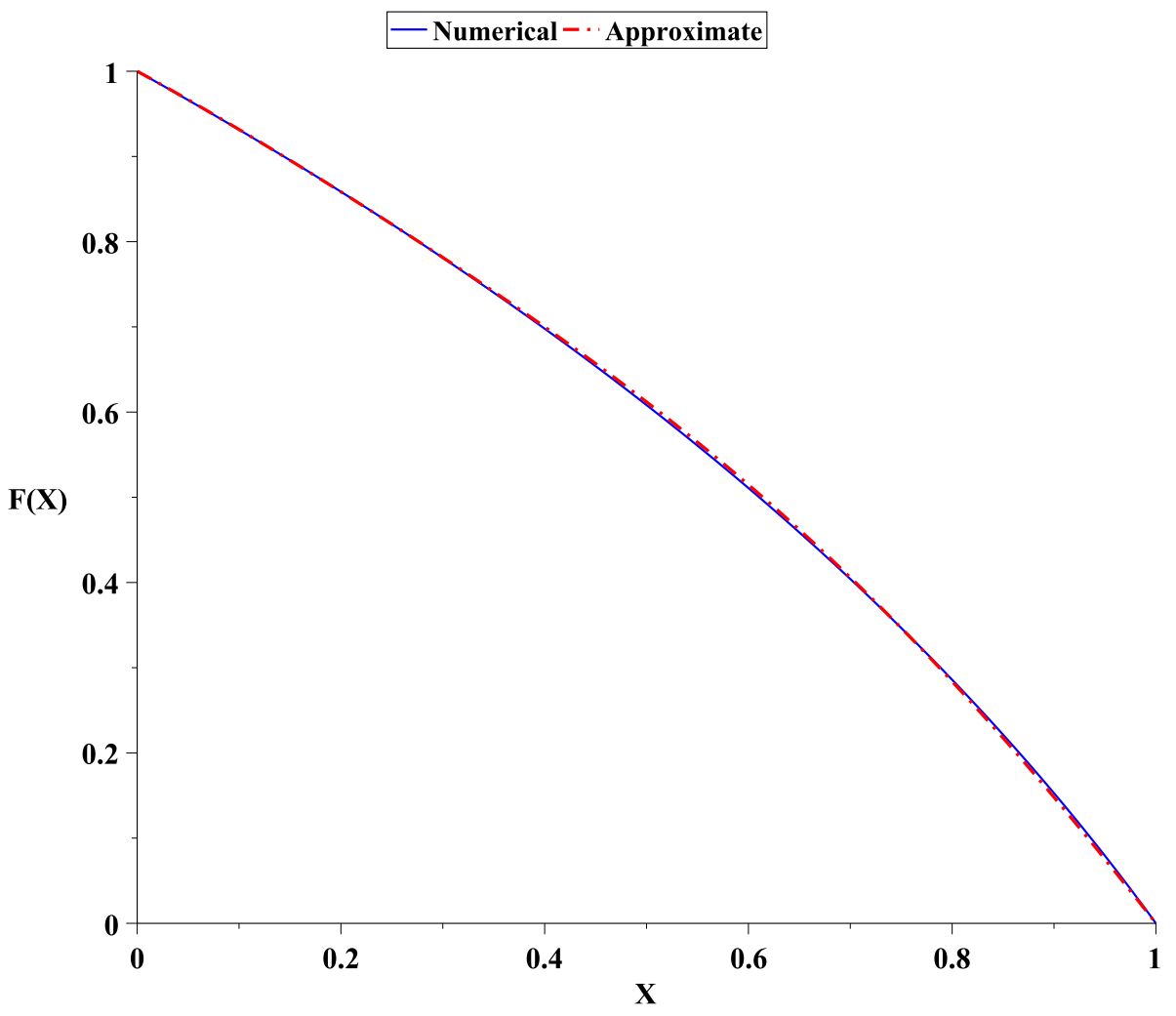
Figure 1. Equation (55) for ε = 0.5 (solid blue line) vs. approximate solution (75) (dash-dot red line).
Mathematics 09 01204 g001
Figure 2. Equation (59) for ε = 0.5 (solid blue line) vs. approximate solution (74) (dash-dot red line).
Mathematics 09 01204 g002
Table 1. Relative errors for (26) and MHPMLT [20].
xy(x) (26)Relative Error Using (26)MHPMLT [20]Relative Error Using MHPMLT [20]
010 %10 %
0.10.92336880.399%0.89999992.9226%
0.20.84220680.7989%0.84398830.5901%
0.30.75705581.10%0.76253960.3855%
0.40.66800621.22%0.67697180.0970%
0.50.57469781.11%0.58590610.8149%
0.60.47631480.7042%0.48796781.7249%
0.70.3715950.0392%0.38178262.7815%
0.80.2588241.11%0.26597593.9355%
0.90.1358322.60%0.13917315.1314%
1.000%00%
Publisher’s Note: MDPI stays neutral with regard to jurisdictional claims in published maps and institutional affiliations.

