
Design Improvement for Complex Systems with Uncertainty


Abstract
1. Introduction
2. Motivation and Problem Statement
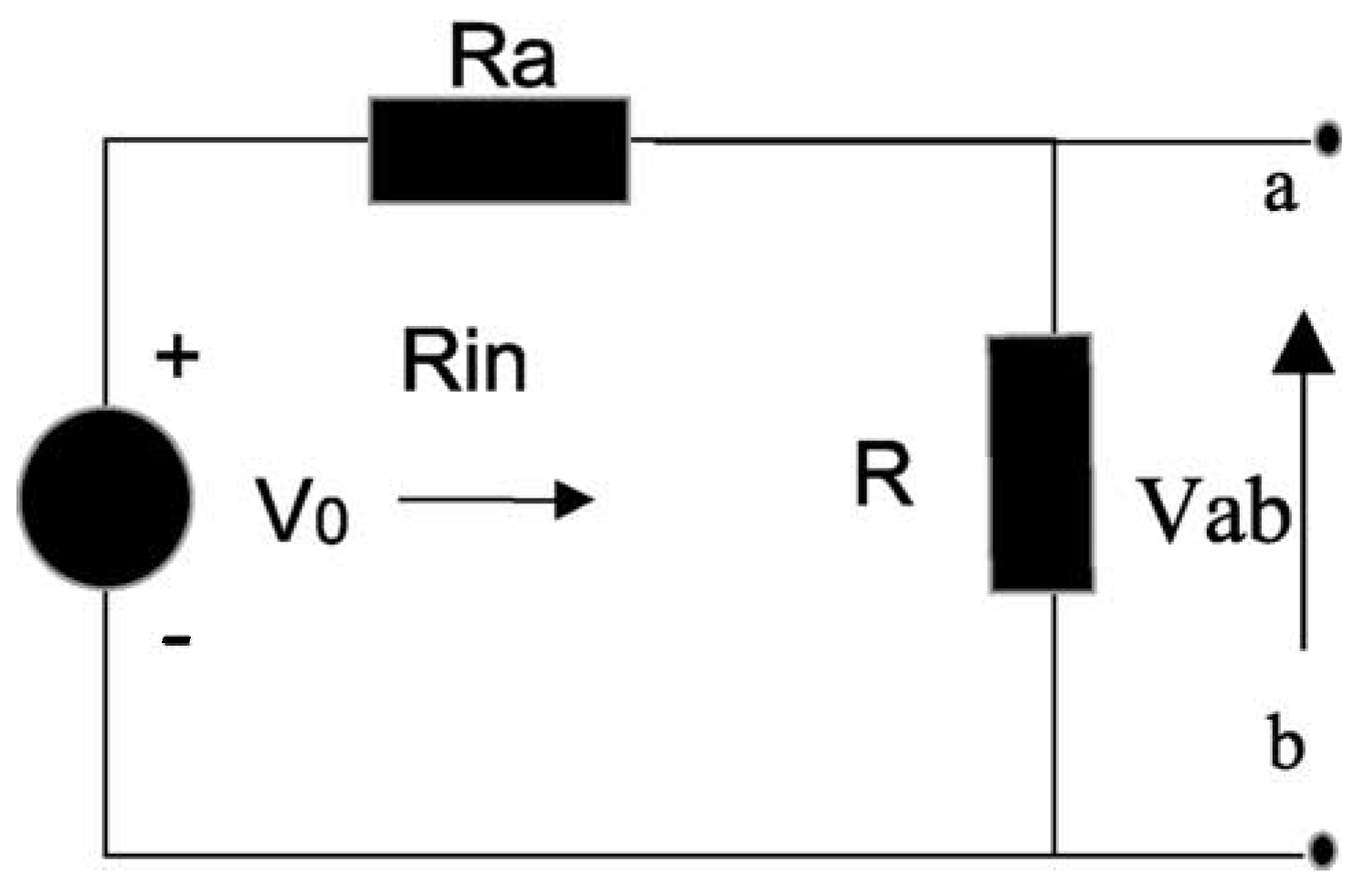
2.1. Motivation
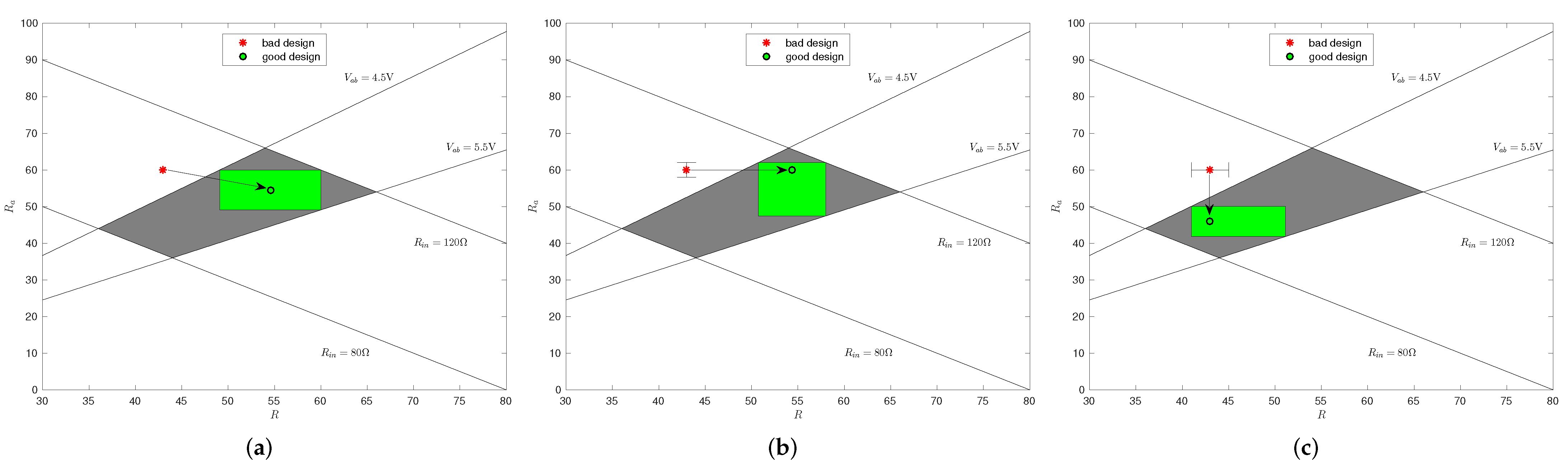
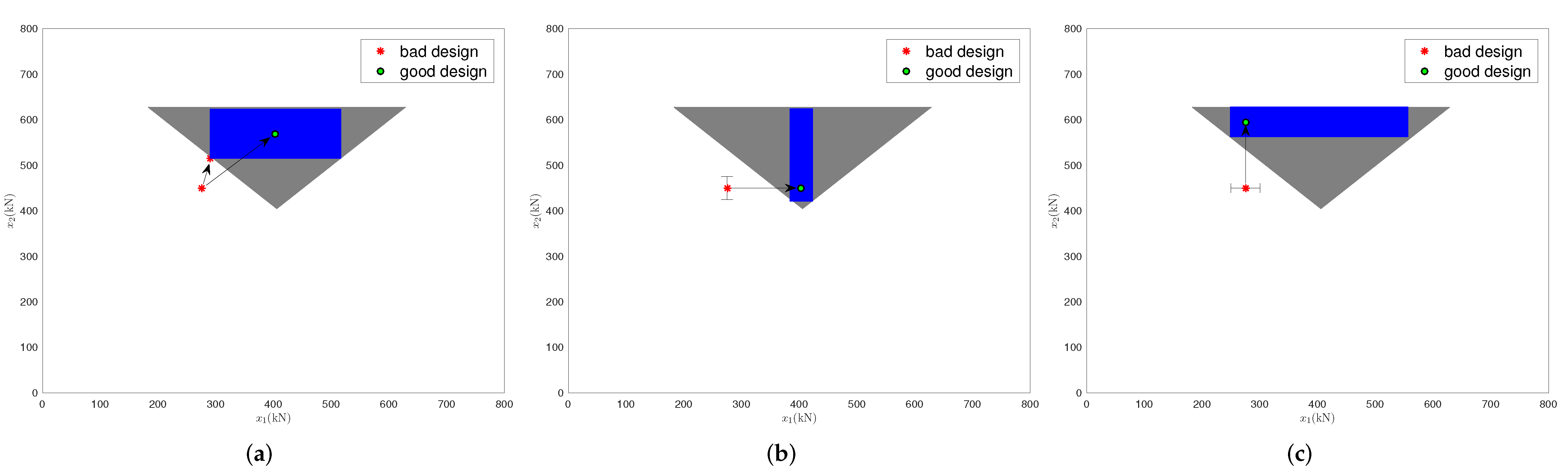
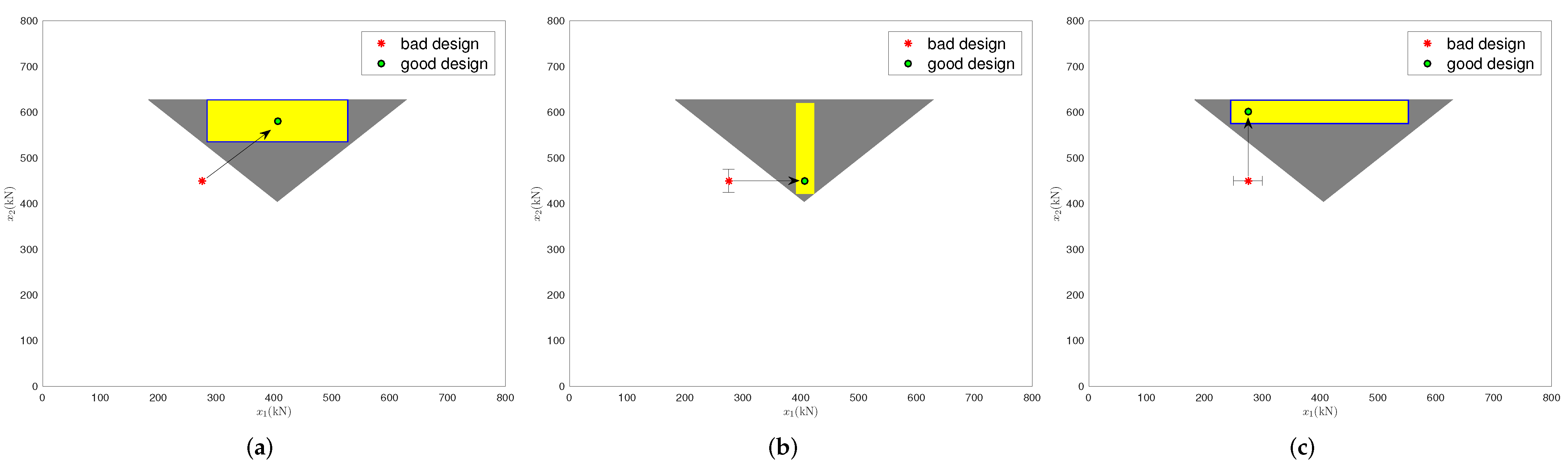
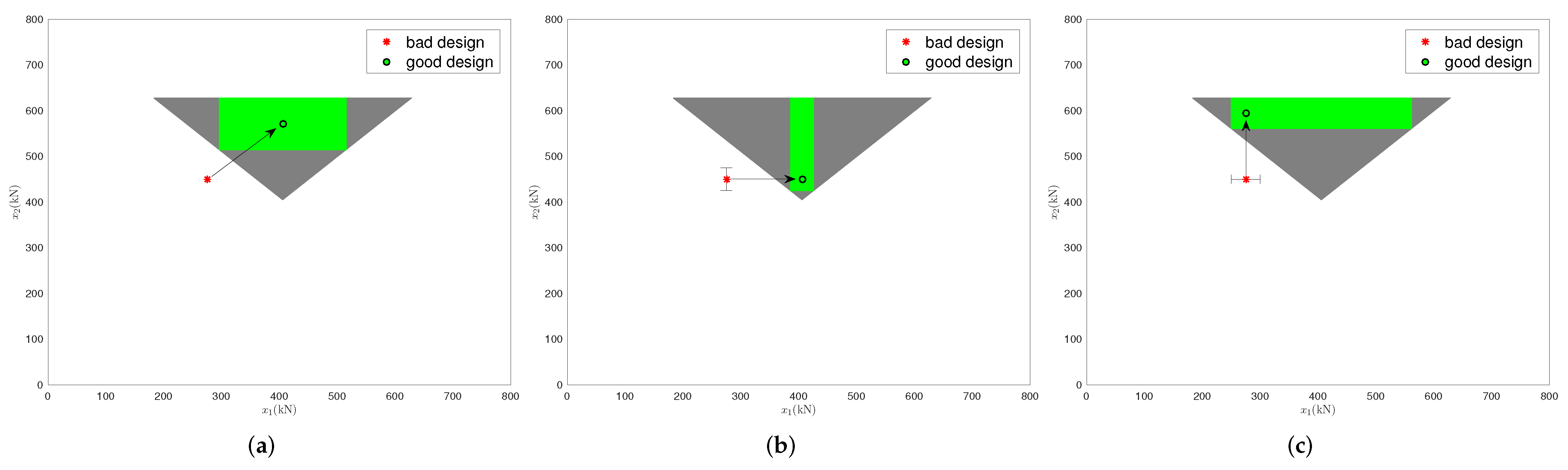
- (a)
- Figure 2a shows a solution hyper-box with the maximum volume. Both R and are changed so as to achieve the design goals.
- (b)
- Figure 2b shows a solution hyper-box that includes . To achieve the design goals, only R needs to be modified. The solution hyper-box is obtained by requiring a minimum safety margin of for . This is essential, because is subject to uncertainty and cannot be controlled exactly. The realized lower safety margin is larger than the required minimum safety margin, thus more tolerance to uncertainty is provided.
- (c)
- Figure 2c shows a solution hyper-box that includes . To realize the design goals, only needs to be modified. The same minimum safety margin as in Scenario (b) is required.
2.2. Problem Statement
3. Preliminaries
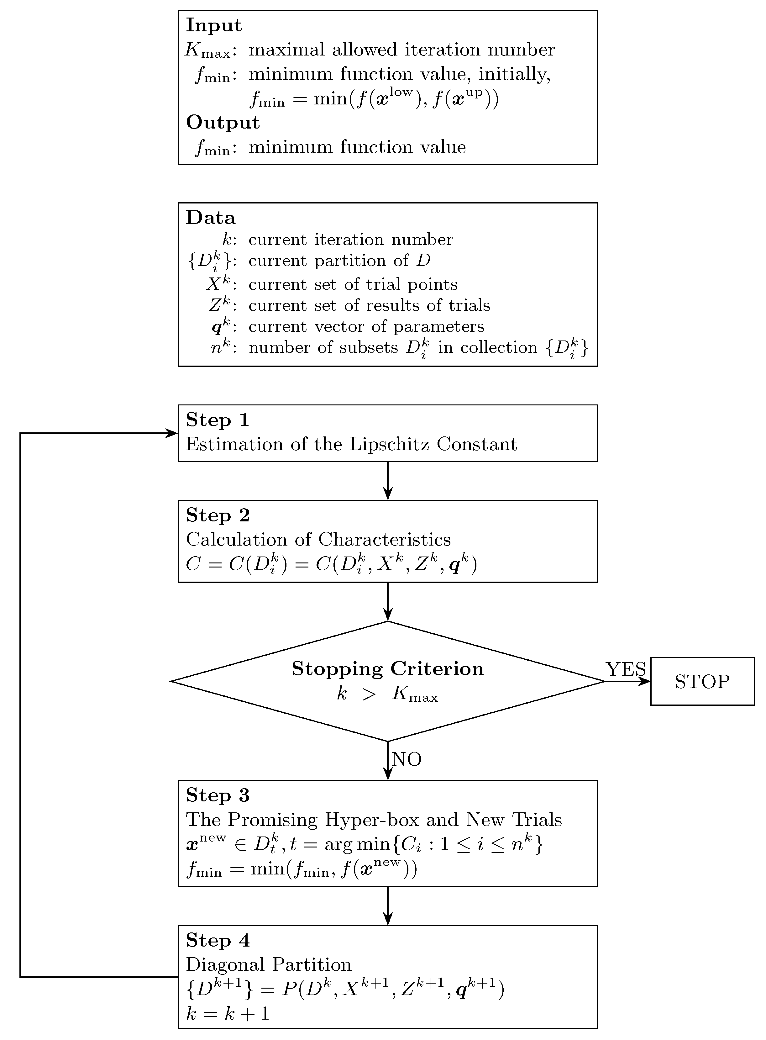
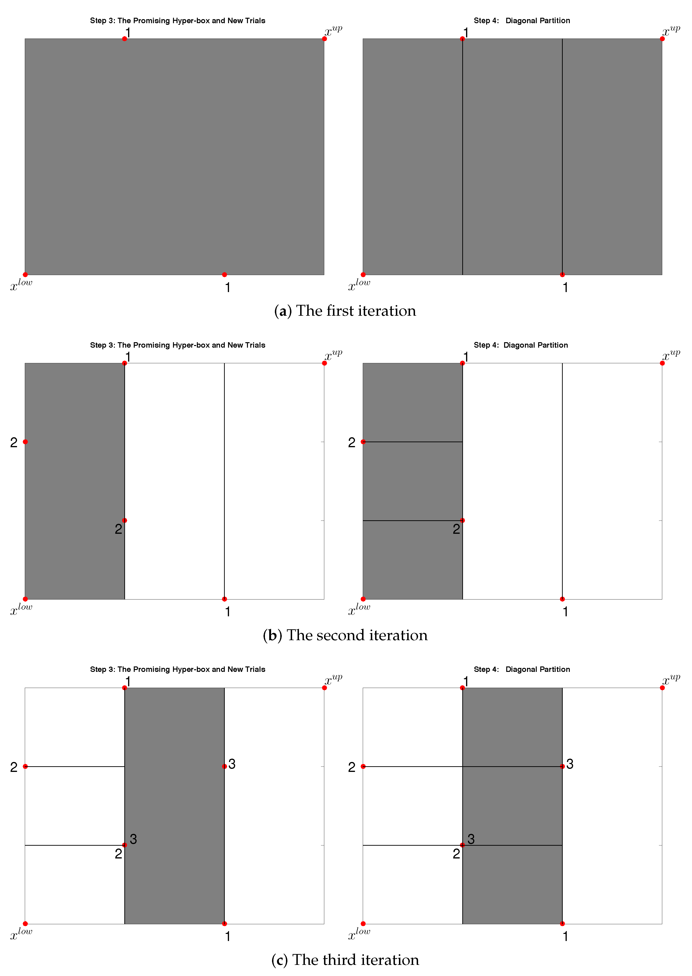
3.1. Divide-the-Best Algorithm
3.2. Particle Swarm Optimization (PSO)
4. The Proposed Particle Swarm Optimization Divide-the-Best Algorithm
| Algorithm 1 The particle swarm optimization divide-the-best algorithm (PSO-Divide-Best) |
|
- (1)
- PSO-Divide-Best has great possibility to reach the globally maximum solution hyper-box satisfying the constraints.
- (2)
- Due to the discrete nature of the trial points in the Divide-the-Best algorithm, the PSO-Divide-Best method can be applied to both analytically known and black-box performance functions.
- (3)
- PSO-Divide-Best guarantees that any point selected within the obtained hyper-box is a good design provided that the performance function is continuous.
5. Case Studies
5.1. Vehicle Structure Design Problem
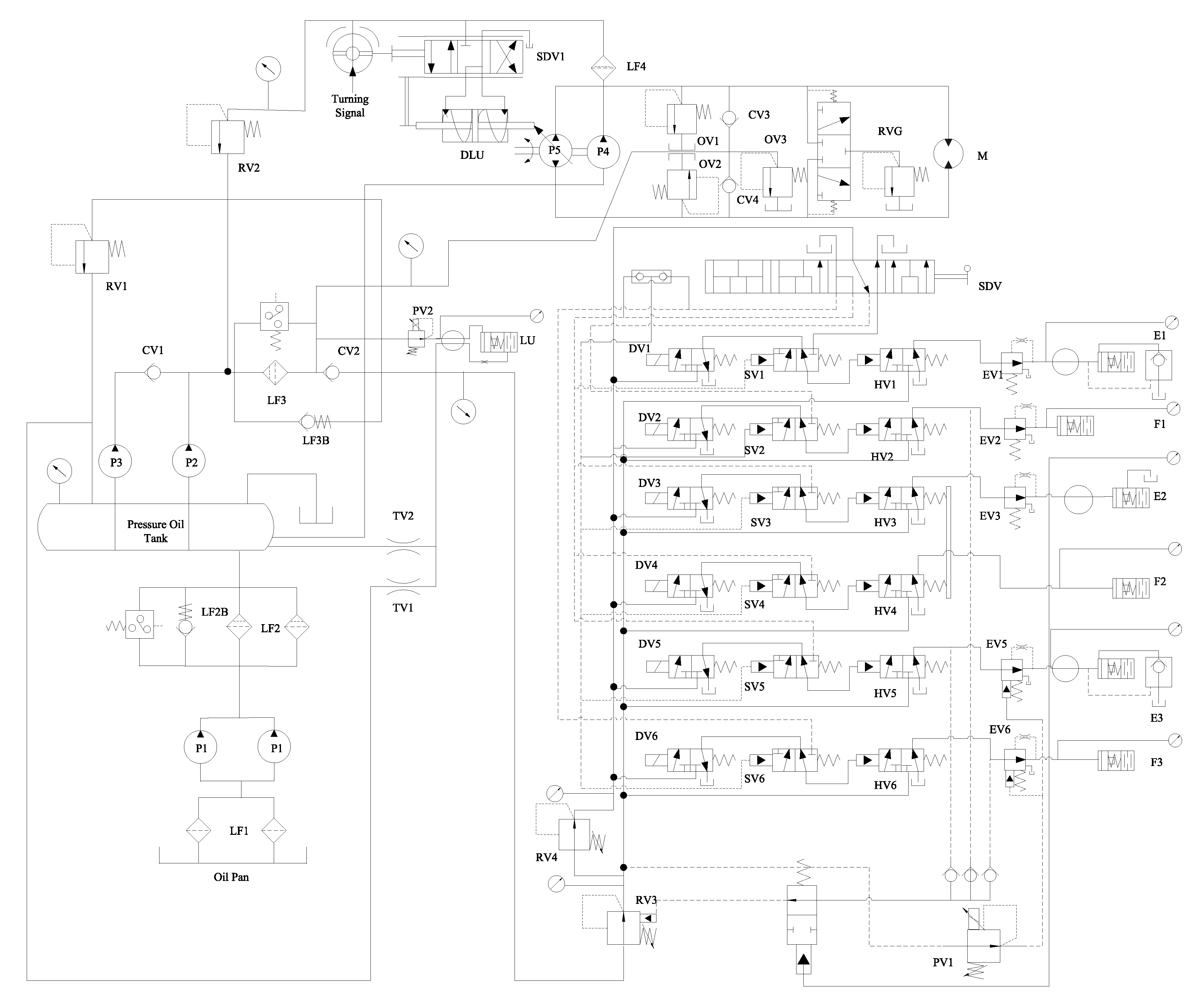
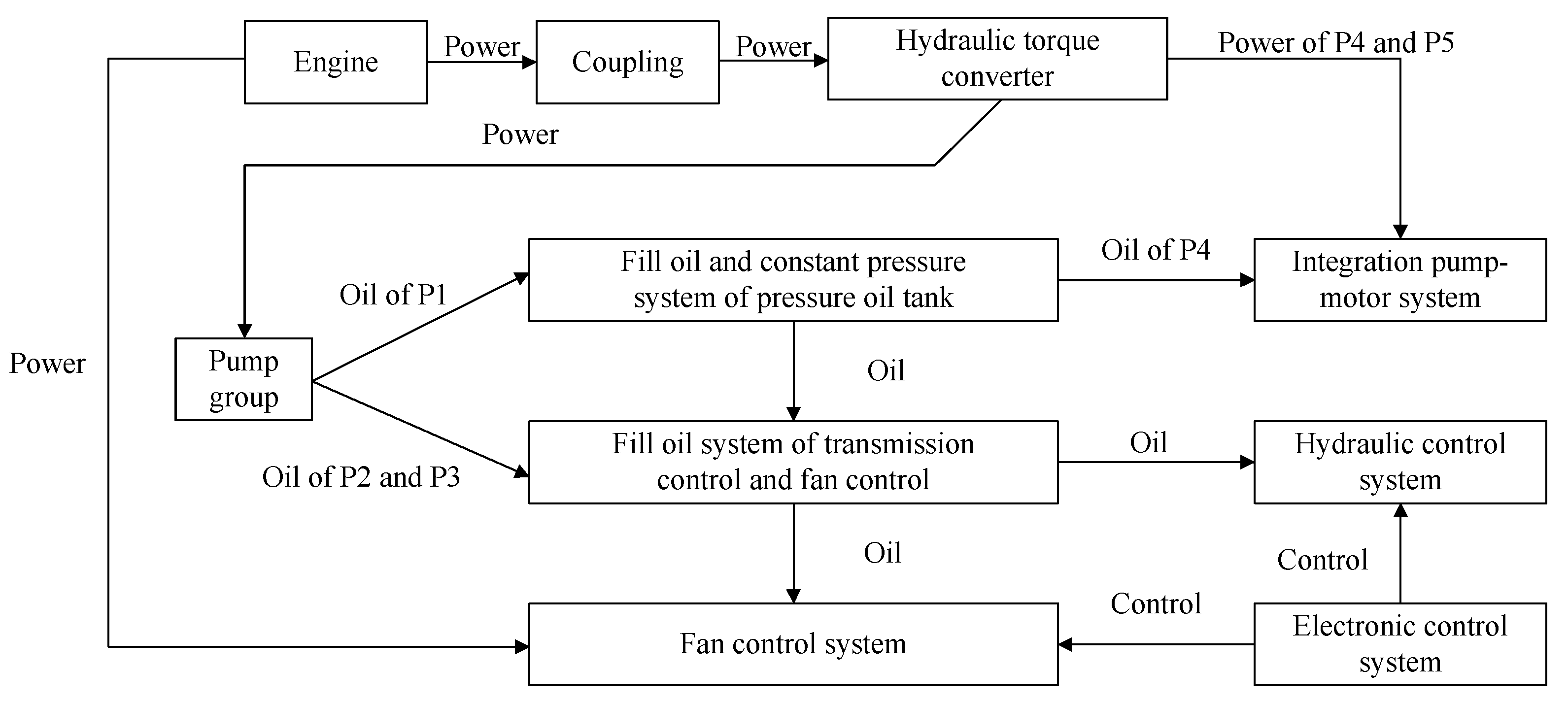
5.2. The Power-Shift Steering Transmission Control System (PSSTCS)
6. Conclusions
Author Contributions
Funding
Institutional Review Board Statement
Informed Consent Statement
Data Availability Statement
Conflicts of Interest
Abbreviations
| PSO | Particle Swarm Optimization |
| PSSTCS | Power-Shift Steering Transmission Control System |
| PSO-Divide-Best | Particle Swarm Optimization Divide-the-Best algorithm |
| EPCP | Approach in [28] including exploration phase and consolidation phase |
| IA-CES | Method in [24] which combines interval arithmetic with cellular evolutionary strategies |
Appendix A

| Bad Design | Good Design | Bad Design | Good Design | ||||
|---|---|---|---|---|---|---|---|
| EPCP | PSO-Divide-Best | EPCP | PSO-Divide-Best | ||||
| 0.9996 | 0.9998 | 0.9999 | 0.9996 | 0.9996 | 0.9996 | ||
| 0.9996 | 0.9996 | 0.9996 | 0.9996 | 0.9996 | 0.9996 | ||
| 0.9996 | 0.9996 | 0.9996 | 0.9996 | 0.9997 | 0.9999 | ||
| 0.9996 | 0.9996 | 0.9998 | 0.9996 | 0.9996 | 0.9996 | ||
| 0.9996 | 0.9997 | 0.9997 | 0.9996 | 0.9996 | 0.9996 | ||
| 0.9996 | 0.9996 | 0.9996 | 0.9996 | 0.9996 | 0.9996 | ||
| 0.9996 | 0.9996 | 0.9996 | 0.9996 | 0.9998 | 0.9996 | ||
| 0.9996 | 0.9996 | 0.9996 | 0.9996 | 0.9996 | 0.9996 | ||
| 0.9996 | 0.9996 | 0.9996 | 0.9996 | 0.9996 | 0.9996 | ||
| 0.9996 | 0.9997 | 0.9998 | 0.9996 | 0.9998 | 0.9999 | ||
| 0.9996 | 0.9998 | 0.9998 | 0.9996 | 0.9996 | 0.9996 | ||
| 0.9996 | 0.9996 | 0.9996 | 0.9996 | 0.9997 | 0.9999 | ||
| 0.9996 | 0.9997 | 0.9998 | 0.9996 | 0.9996 | 0.9996 | ||
| 0.9996 | 0.9997 | 0.9999 | 0.9996 | 0.9996 | 0.9996 | ||
| 0.9996 | 0.9997 | 0.9998 | 0.9996 | 0.9996 | 0.9996 | ||
| 0.9996 | 0.9996 | 0.9996 | 0.9996 | 0.9996 | 0.9996 | ||
| 0.9996 | 0.9997 | 0.9999 | 0.9996 | 0.9998 | 0.9999 | ||
| 0.9996 | 0.9996 | 0.9996 | 0.9996 | 0.9996 | 0.9996 | ||
| 0.9996 | 0.9996 | 0.9996 | 0.9996 | 0.9996 | 0.9996 | ||
| 0.9996 | 0.9996 | 0.9996 | 0.9996 | 0.9998 | 0.9998 | ||
| 0.9996 | 0.9998 | 0.9998 | 0.9996 | 0.9996 | 0.9996 | ||
| 0.9996 | 0.9996 | 0.9996 | 0.9996 | 0.9998 | 0.9999 | ||
| 0.9996 | 0.9996 | 0.9996 | 0.9996 | 0.9998 | 0.9998 | ||
| 0.9996 | 0.9997 | 0.9999 | 0.9996 | 0.9998 | 0.9998 | ||
| 0.9996 | 0.9998 | 0.9999 | 0.9996 | 0.9997 | 0.9999 | ||
| 0.9996 | 0.9996 | 0.9996 | 0.9996 | 0.9997 | 0.9998 | ||
| 0.9996 | 0.9998 | 0.9997 | 0.9996 | 0.9998 | 0.9999 | ||
| 0.9996 | 0.9996 | 0.9996 | 0.9996 | 0.9996 | 0.9996 | ||
| 0.9996 | 0.9996 | 0.9996 | 0.9996 | 0.9996 | 0.9997 | ||
| 0.9996 | 0.9996 | 0.9996 | 0.9996 | 0.9996 | 0.9997 | ||
| 0.9996 | 0.9997 | 0.9999 | 0.9996 | 0.9997 | 0.9998 | ||
| 0.9996 | 0.9997 | 0.9995 | 0.9996 | 0.9997 | 0.9998 | ||
| 0.9996 | 0.9996 | 0.9996 | 0.9996 | 0.9996 | 0.9996 | ||
| 0.9996 | 0.9997 | 0.9997 | 0.9996 | 0.9996 | 0.9996 | ||
| 0.9996 | 0.9996 | 0.9996 | 0.9996 | 0.9996 | 0.9995 | ||
| 0.9996 | 0.9996 | 0.9996 | 0.9996 | 0.9996 | 0.9996 | ||
| 0.9996 | 0.9996 | 0.9996 | 0.9996 | 0.9997 | 0.9996 | ||
| 0.9996 | 0.9997 | 0.9997 | 0.9996 | 0.9997 | 0.9998 | ||
| 0.9996 | 0.9997 | 0.9997 | 0.9996 | 0.9996 | 0.9998 | ||
| 0.9996 | 0.9997 | 0.9998 | 0.9996 | 0.9997 | 0.9995 | ||
| 0.9996 | 0.9997 | 0.9997 | 0.9996 | 0.9996 | 0.9996 | ||
| 0.9996 | 0.9996 | 0.9996 | 0.9996 | 0.9997 | 0.9996 | ||
| 0.9996 | 0.9996 | 0.9995 | 0.9996 | 0.9998 | 0.9998 | ||
| 0.9856 | 0.9912 | 0.9940 | |||||
| Lower Bound | EPCP | PSO-Divide-Best | Upper Bound | EPCP | PSO-Divide-Best |
|---|---|---|---|---|---|
| 0.9997 | 0.9997 | 0.9999 | 1.0000 | ||
| 0.9995 | 0.9994 | 0.9998 | 1.0000 | ||
| 0.9996 | 0.9991 | 0.9998 | 1.0000 | ||
| 0.9995 | 0.9993 | 0.9998 | 1.0000 | ||
| 0.9995 | 0.9995 | 0.9998 | 1.0000 | ||
| 0.9997 | 0.9997 | 0.9998 | 1.0000 | ||
| 0.9995 | 0.9995 | 0.9997 | 1.0000 | ||
| 0.9995 | 0.9992 | 0.9998 | 1.0000 | ||
| 0.9996 | 0.9994 | 0.9998 | 1.0000 | ||
| 0.9995 | 0.9999 | 0.9999 | 1.0000 | ||
| 0.9990 | 0.9990 | 1.0000 | 1.0000 | ||
| 0.9990 | 0.9990 | 1.0000 | 1.0000 | ||
| 0.9991 | 0.9990 | 1.0000 | 1.0000 | ||
| 0.9997 | 0.9998 | 0.9999 | 1.0000 | ||
| 0.9995 | 0.9992 | 0.9998 | 1.0000 | ||
| 0.9996 | 0.9994 | 0.9998 | 1.0000 | ||
| 0.9997 | 0.9994 | 0.9999 | 1.0000 | ||
| 0.9995 | 0.9995 | 0.9999 | 1.0000 | ||
| 0.9995 | 0.9996 | 0.9999 | 1.0000 | ||
| 0.9997 | 0.9998 | 0.9999 | 1.0000 | ||
| 0.9997 | 0.9997 | 0.9999 | 1.0000 | ||
| 0.9997 | 0.9998 | 0.9999 | 1.0000 | ||
| 0.9990 | 0.9990 | 1.0000 | 1.0000 | ||
| 0.9995 | 0.9999 | 0.9998 | 1.0000 | ||
| 0.9995 | 0.9995 | 0.9999 | 1.0000 | ||
| 0.9997 | 0.9998 | 0.9999 | 1.0000 | ||
| 0.9995 | 0.9998 | 0.9999 | 1.0000 | ||
| 0.9990 | 0.9990 | 1.0000 | 1.0000 | ||
| 0.9995 | 0.9995 | 0.9999 | 1.0000 | ||
| 0.9997 | 0.9995 | 0.9999 | 1.0000 | ||
| 0.9990 | 0.9990 | 1.0000 | 1.0000 | ||
| 0.9990 | 0.9990 | 1.0000 | 1.0000 | ||
| 0.9995 | 0.9997 | 0.9999 | 1.0000 | ||
| 0.9997 | 0.9999 | 0.9999 | 1.0000 | ||
| 0.9990 | 0.9990 | 1.0000 | 1.0000 | ||
| 0.9991 | 0.9990 | 1.0000 | 1.0000 | ||
| 0.9991 | 0.9990 | 1.0000 | 1.0000 | ||
| 0.9992 | 0.9990 | 1.0000 | 1.0000 | ||
| 0.9990 | 0.9990 | 1.0000 | 1.0000 | ||
| 0.9997 | 0.9995 | 0.9999 | 1.0000 | ||
| 0.9997 | 0.9997 | 0.9999 | 1.0000 | ||
| 0.9995 | 0.9995 | 0.9999 | 1.0000 | ||
| 0.9997 | 0.9997 | 0.9999 | 1.0000 | ||
| 0.9997 | 0.9999 | 0.9999 | 1.0000 | ||
| 0.9998 | 0.9998 | 0.9999 | 1.0000 | ||
| 0.9997 | 0.9995 | 0.9999 | 1.0000 | ||
| 0.9995 | 0.9998 | 0.9999 | 1.0000 | ||
| 0.9997 | 0.9995 | 0.9999 | 1.0000 | ||
| 0.9997 | 0.9999 | 0.9999 | 1.0000 | ||
| 0.9995 | 0.9998 | 0.9999 | 1.0000 | ||
| 0.9996 | 0.9995 | 0.9998 | 1.0000 | ||
| 0.9995 | 0.9995 | 0.9998 | 1.0000 | ||
| 0.9997 | 0.9995 | 0.9999 | 1.0000 | ||
| 0.9997 | 0.9998 | 0.9999 | 1.0000 | ||
| 0.9997 | 0.9995 | 0.9999 | 1.0000 | ||
| 0.9997 | 0.9995 | 0.9999 | 1.0000 | ||
| 0.9996 | 0.9992 | 0.9998 | 1.0000 | ||
| 0.9995 | 0.9994 | 0.9998 | 1.0000 | ||
| 0.9996 | 0.9994 | 0.9998 | 1.0000 | ||
| 0.9995 | 0.9994 | 0.9998 | 1.0000 | ||
| 0.9996 | 0.9997 | 0.9998 | 1.0000 | ||
| 0.9996 | 0.9996 | 0.9998 | 1.0000 | ||
| 0.9995 | 0.9990 | 0.9998 | 1.0000 | ||
| 0.9996 | 0.9996 | 0.9998 | 1.0000 | ||
| 0.9996 | 0.9995 | 0.9998 | 1.0000 | ||
| 0.9995 | 0.9995 | 0.9998 | 1.0000 | ||
| 0.9995 | 0.9994 | 0.9998 | 1.0000 | ||
| 0.9996 | 0.9994 | 0.9998 | 1.0000 | ||
| 0.9996 | 0.9990 | 0.9998 | 1.0000 | ||
| 0.9995 | 0.9990 | 0.9998 | 1.0000 | ||
| 0.9995 | 0.9990 | 0.9998 | 1.0000 | ||
| 0.9995 | 0.9995 | 0.9998 | 1.0000 | ||
| 0.9996 | 0.9992 | 0.9998 | 1.0000 | ||
| 0.9995 | 0.9991 | 0.9998 | 1.0000 | ||
| 0.9995 | 0.9994 | 0.9998 | 1.0000 | ||
| 0.9996 | 0.9995 | 0.9998 | 1.0000 | ||
| 0.9995 | 0.9993 | 0.9998 | 1.0000 | ||
| 0.9995 | 0.9995 | 0.9998 | 1.0000 | ||
| 0.9996 | 0.9995 | 0.9998 | 1.0000 | ||
| 0.9996 | 0.9990 | 0.9998 | 1.0000 | ||
| 0.9996 | 0.9994 | 0.9998 | 1.0000 | ||
| 0.9996 | 0.9993 | 0.9998 | 1.0000 | ||
| 0.9996 | 0.9996 | 0.9998 | 1.0000 | ||
| 0.9996 | 0.9992 | 0.9998 | 1.0000 | ||
| 0.9995 | 0.9990 | 0.9998 | 1.0000 | ||
| 0.9997 | 0.9995 | 0.9999 | 1.0000 |
References
- Oberkampf, W.L. Uncertainty Quantification Using Evidence Theory; Stanford University: Stanford, CA, USA, 2005. [Google Scholar]
- Lim, D.; Ong, Y.S.; Sendhoff, B.; Lee, B.S. Inverse multi-objective robust evolutionary design optimization. Genet. Program. Evolvable Mach. 2007, 7, 383–404. [Google Scholar] [CrossRef][Green Version]
- Li, M.Y.; Zhang, W.D.; Hu, Q.P.; Guo, H.R.; Liu, J. Design and Risk Evaluation of Reliability Demonstration Test for Hierarchical Systems With Multilevel Information Aggregation. IEEE Trans. Reliab. 2017, 66, 135–147. [Google Scholar] [CrossRef]
- Zhao, Y.G.; Ono, T. A general procedure for first/second-order reliability method (FORM/SORM). Struct. Saf. 1999, 21, 95–112. [Google Scholar] [CrossRef]
- Saltelli, A.; Scott, M. Guest editorial: The role of sensitivity analysis in the corroboration of models and its link to model structural and parametric uncertainty. Reliab. Eng. Syst. Saf. 1997, 57, 1–4. [Google Scholar] [CrossRef]
- Pannier, S.; Graf, W. Sensitivity measures for fuzzy numbers based on artificial neural networks. In Applications of Statistics and Probability in Civil Engineering; CRC Press: London, UK, 2011; pp. 497–505. [Google Scholar]
- Taguchi, G.; Elsayed, E.; Hsiang, T. Quality Engineering in Production Systems; McGraw-Hill: New York, NY, USA, 1989. [Google Scholar]
- Hara, K.; Inoue, M. Gain-Preserving Data-Driven Approximation of the Koopman Operator and Its Application in Robust Controller Design. Mathematics 2021, 9, 949. [Google Scholar] [CrossRef]
- Lee, M.; Jeong, H.; Lee, D. Design Optimization of 3-DOF Redundant Planar Parallel Kinematic Mechanism Based Finishing Cut Stage for Improving Surface Roughness of FDM 3D Printed Sculptures. Mathematics 2021, 9, 961. [Google Scholar] [CrossRef]
- Gunawan, S.; Papalambros, P.Y. A Bayesian Approach to Reliability-Based Optimization With Incomplete Information. J. Mech. Des. 2006, 128, 909–918. [Google Scholar] [CrossRef]
- Stocki, R. A method to improve design reliability using optimal Latin hypercube sampling. Comput. Assist. Mech. Eng. Sci. 2005, 12, 393–411. [Google Scholar]
- Lehar, M.; Zimmermann, M. An inexpensive estimate of failure probability for high-dimensional systems with uncertainty. Struct. Saf. 2012, 36–37, 32–38. [Google Scholar] [CrossRef]
- Daum, D.A.; Deb, K.; Branke, J. Reliability-based optimization for multiple constraints with evolutionary algorithms. In Proceedings of the 2007 IEEE Congress on Evolutionary Computation, Singapore, 25–28 September 2007. [Google Scholar]
- Asafuddoula, M.; Singh, H.K.; Ray, T. Six-Sigma Robust Design Optimization Using a Many-Objective Decomposition-Based Evolutionary Algorithm. IEEE Trans. Evol. Comput. 2015, 19, 490–507. [Google Scholar] [CrossRef]
- Jin, Y.; Branke, J. Evolutionary optimization in uncertain environments—A survey. IEEE Trans. Evol. Comput. 2005, 9, 303–317. [Google Scholar] [CrossRef]
- Nguyen, T.T.; Yang, S.; Branke, J. Evolutionary dynamic optimization: A survey of the state of the art. Swarm Evol. Comput. 2012, 6, 1–24. [Google Scholar] [CrossRef]
- Knight, J.T.; Zahradka, F.T.; Singer, D.J.; Collette, M. Multiobjective Particle Swarm Optimization of a Planing Craft with Uncertainty. J. Ship Prod. Des. 2018, 30, 194–200. [Google Scholar] [CrossRef]
- Fan, X.N.; Yue, X.Y.; Li, Y.Z. LHS applied to reliability-based design optimization of a crane metallic structure. J. Chem. Pharm. Res. 2015, 7, 2400–2406. [Google Scholar]
- Qin, Y.; Zhu, J.F.; Wei, Z. The robust optimization of the capacitated hub and spoke airline network design base on ant colony algorithms. In Proceedings of the 2010 International Conference on Intelligent Computing and Integrated Systems, Guilin, China, 22–24 October 2010; pp. 601–604. [Google Scholar]
- Chen, T.H.; Yeh, M.F.; Lee, W.Y.; Hsieh, W.H. Particle swarm optimization based networked control system design with uncertainty. Matec Web Conf. 2017, 119, 01051. [Google Scholar] [CrossRef]
- Zimmermann, M.; von Hoessle, J.E. Computing solution spaces for robust design. Int. J. Numer. Methods Eng. 2013, 94, 290–307. [Google Scholar] [CrossRef]
- Zimmermann, M. Vehicle Front Crash Design Accounting for Uncertainties. In Proceedings of the FISITA 2012 World Automotive Congress; Springer: Berlin/Heidelberg, Germany, 2013; Volume 197, pp. 83–89. [Google Scholar]
- Graff, L.; Harbrecht, H.; Zimmermann, M. On the computation of solution spaces in high dimensions. Struct. Multidiscip. Optim. 2016, 54, 811–829. [Google Scholar] [CrossRef]
- Rocco, C.M.; Moreno, J.A.; Carrasquero, N. Robust design using a hybrid cellular-evolutionary and interval-arithmetic approach:a reliability application. Reliab. Eng. Syst. Saf. 2003, 79, 149–159. [Google Scholar] [CrossRef]
- Chen, Y.; Shi, J.; Yi, X.J. A New Reliable Operating Region Design Method. Math. Probl. Eng. 2020, 2020, 1–12. [Google Scholar] [CrossRef]
- Chen, Y.; Shi, J.; Yi, X.J. A globally optimal robust design method for complex systems. Complexity 2020, 2020, 1–25. [Google Scholar] [CrossRef]
- Jones, D.R.; Perttunen, C.D.; Stuckman, B.E. Lipschitzian optimization without the Lipschitz constant. J. Optim. Theory Appl. 1993, 79, 157–181. [Google Scholar] [CrossRef]
- Fender, J.; Graff, L.; Harbrecht, H.; Zimmermann, M. Identifying Key Parameters for Design Improvement in High-Dimensional Systems With Uncertainty. J. Mech. Des. 2014, 136, 041007. [Google Scholar] [CrossRef]
- Kennedy, J. The particle swarm: Social adaptation of knowledge. In Proceedings of the 1997 IEEE International Conference on Evolutionary Computation, Indianapolis, IN, USA, 13–16 April 1997. [Google Scholar]
- Sergeyev, Y.D.; Kvasov, D.E. Global search based on diagonal partitions and a set of Lipschitz constants. SIAM J. Optim. 2006, 16, 910–937. [Google Scholar] [CrossRef]
- Kvasov, D.E.; Sergeyev, Y.D. Multidimensional Global Optimization Algorithm Based on Adaptive Diagonal Curves. Comput. Math. Math. Phys. 2003, 43, 42–59. [Google Scholar]
- Strongin, R.G.; Sergeyev, Y.D. Global Optimization with Non-Convex Constraints. Sequential and Parallel Algorithms; Springer: Berlin/Heidelberg, Germany, 2000. [Google Scholar]
- Sergeyev, Y.D.; Yaroslav, D. An Information Global Optimization Algorithm with Local Tuning. SIAM J. Optim. 2006, 5, 858–870. [Google Scholar] [CrossRef]
- Kvasov, D.E.; Sergeyev, Y.D. Deterministic approaches for solving practical black-box global optimization problems. Adv. Eng. Softw. 2015, 80, 58–66. [Google Scholar] [CrossRef]
- Sergeyev, Y.D.; Kvasov, D.E. A deterministic global optimization using smooth diagonal auxiliary functions. Commun. Nonlinear Sci. Numer. Simul. 2015, 21, 99–111. [Google Scholar] [CrossRef]
- Gablonsky, J.M. Modifications of the Direct Algorithm. Ph.D. Thesis, North Carolina State University, Raleigh, NC, USA, 2001. [Google Scholar]
- Paulavicius, R.; Chiter, L.; Žilinskas, J. Global optimization based on bisection of rectangles, function values at diagonals, and a set of Lipschitz constants. J. Glob. Optim. 2018, 71, 5–20. [Google Scholar] [CrossRef]
- Paulavičius, R.; Žilinskas, J.; Grothey, A. Investigation of selection strategies in branch and bound algorithm with simplicial partitions and combination of Lipschitz bounds. Optim. Lett. 2010, 4, 173–183. [Google Scholar] [CrossRef]
- Stripinis, L.; Paulavičius, R.; Žilinskas, J. Improved scheme for selection of potentially optimal hyper-rectangles in DIRECT. Optim. Lett. 2018, 12, 1699–1712. [Google Scholar] [CrossRef]
- Yan, J.; Hu, T.; Huang, C.C.; Wu, X. An improved particle swarm optimization algorithm. Adv. Mater. Res. 2009, 195–196, 1060–1065. [Google Scholar]
- Barrera, J.; Coello, C. A Review of Particle Swarm Optimization Methods Used for Multimodal Optimization. In Innovations in Swarm Intelligence; Springer: Berlin/Heidelberg, Germany, 2009. [Google Scholar]
- Gandomi, A.H.; Yun, G.J.; Yang, X.S.; Talatahari, S. Chaos-enhanced accelerated particle swarm optimization. Commun. Nonlinear Sci. Numer. Simul. 2013, 18, 327–340. [Google Scholar] [CrossRef]
- Rao, S.S. Engineering Optimization Theory and Practice; John Wiley & Sons, Inc.: Hoboken, NJ, USA, 2009. [Google Scholar]
- Kuhn, H.W.; Tucker, A.W. Nonlinear programming. In Proceedings of 2nd Berkeley Symposium; University of California Press: Berkeley, CA, USA, 1951; pp. 481–492. [Google Scholar]
- Yi, X.J.; Shi, J.; Dhillon, B.S.; Hou, P.; Dong, H.P. A new reliability analysis method for repairable systems with closed-loop feedback links. Qual. Reliab. Eng. Int. 2018, 34, 298–332. [Google Scholar] [CrossRef]


| (a) Both and Are Key Parameters | (b) Only Is Key Parameter | (c) Only Is Key Parameter | ||||||||||
|---|---|---|---|---|---|---|---|---|---|---|---|---|
| kN | kN | |||||||||||
| kN | kN | |||||||||||
| exact | EPCP | IA-CES | PSO-Divide-Best | exact | EPCP | IA-CES | PSO-Divide-Best | exact | EPCP | IA-CES | PSO-Divide-Best | |
| (kN) | 294.80 | 290.74 | 284.08 | 296.15 | 386.20 | 384.30 | 392.53 | 386.20 | 250.00 | 249.14 | 245.05 | 250.00 |
| (kN) | 516.40 | 516.31 | 527.30 | 515.06 | 425.00 | 422.47 | 422.78 | 425.00 | 561.20 | 556.32 | 552.28 | 561.47 |
| (kN) | 516.40 | 515.81 | 535.46 | 515.06 | 425.00 | 422.06 | 422.78 | 425.00 | 561.20 | 563.67 | 575.21 | 561.47 |
| (kN) | 627.20 | 622.59 | 626.95 | 627.20 | 627.20 | 623.69 | 619.36 | 627.19 | 627.20 | 627.48 | 626.38 | 627.19 |
| volume (kN) | 2.4553 | 2.4086 | 2.2253 | 2.4548 | 0.7845 | 0.7696 | 0.5756 | 0.7844 | 2.0539 | 1.9601 | 1.5721 | 2.0537 |
| (%) | ____ | 1.38 | 3.64 | 0.46 | ____ | 0.49 | 1.64 | 0.00 | ____ | 0.34 | 1.59 | 0.00 |
| (%) | ____ | 0.02 | 2.11 | 0.26 | ____ | 0.60 | 0.75 | 0.00 | ____ | 0.87 | 1.98 | 0.05 |
| (%) | ____ | 0.11 | 3.69 | 0.26 | ____ | 0.69 | 1.25 | 0.00 | ____ | 0.44 | 2.50 | 0.05 |
| (%) | ____ | 0.74 | 0.04 | 0.00 | ____ | 0.56 | 0.52 | 0.01 | ____ | 0.04 | 0.13 | 0.00 |
| error (%) | ____ | 1.90 | 9.29 | 0.02 | ____ | 1.90 | 26.63 | 0.01 | ____ | 4.57 | 23.46 | 0.01 |
| Method | EPCP | PSO-Divide-Best |
|---|---|---|
| Log-volume | −698.6824 | −656.9503 |
Publisher’s Note: MDPI stays neutral with regard to jurisdictional claims in published maps and institutional affiliations. |
© 2021 by the authors. Licensee MDPI, Basel, Switzerland. This article is an open access article distributed under the terms and conditions of the Creative Commons Attribution (CC BY) license (https://creativecommons.org/licenses/by/4.0/).
Share and Cite
Chen, Y.; Shi, J.; Yi, X.-J. Design Improvement for Complex Systems with Uncertainty. Mathematics 2021, 9, 1173. https://doi.org/10.3390/math9111173
Chen Y, Shi J, Yi X-J. Design Improvement for Complex Systems with Uncertainty. Mathematics. 2021; 9(11):1173. https://doi.org/10.3390/math9111173
Chicago/Turabian StyleChen, Yue, Jian Shi, and Xiao-Jian Yi. 2021. "Design Improvement for Complex Systems with Uncertainty" Mathematics 9, no. 11: 1173. https://doi.org/10.3390/math9111173
APA StyleChen, Y., Shi, J., & Yi, X.-J. (2021). Design Improvement for Complex Systems with Uncertainty. Mathematics, 9(11), 1173. https://doi.org/10.3390/math9111173