Hybrid Model for Time Series of Complex Structure with ARIMA Components

Abstract

A hybrid model for the time series of complex structure (HMTS) was proposed. It is based on the combination of function expansions in a wavelet series with ARIMA models. HMTS has regular and anomalous components. The time series components, obtained after expansion, have a simpler structure that makes it possible to identify the ARIMA model if the components are stationary. This allows us to obtain a more accurate ARIMA model for a time series of complicated structure and to extend the area for application. To identify the HMTS anomalous component, threshold functions are applied. This paper describes a technique to identify HMTS and proposes operations to detect anomalies. With the example of an ionospheric parameter time series, we show the HMTS efficiency, describe the results and their application in detecting ionospheric anomalies. The HMTS was compared with the nonlinear autoregression neural network NARX, which confirmed HMTS efficiency.

1. Introduction

Time series modeling and analysis are important bases for the methods of studying the processes and phenomena of different natures. They are used in various spheres of human activity (physics, biology, medicine, economics, etc.). Methods of data modeling and analysis aimed at detecting and identifying anomalies are of special actuality. The examples are the problems of the recognition of anomalies in geophysical monitoring data, such as the detection of magnetic and ionospheric storms [1,2,3,4], earthquakes [5,6], tsunamis [7,8], geological anomalies [9] and other catastrophic natural phenomena. The need to detect anomalies often arises in the medical field, for example, to detect and to identify clinical conditions of patients [10]. An important property of such methods is their ability to adapt, providing the possibility to detect and identify rapid changes in the system or object state, indicating anomaly occurrences.

As a rule, time series of empirical data have a complex non-stationary structure and contain local features of various forms. The methods for the time series analysis include deterministic [11], stochastic [12,13,14] approaches and their various combinations [15,16,17,18,19]. Traditional methods for data time series modeling and analysis (AR models, ARMA [20,21], exponential smoothing [22], stochastic approximation [13], etc.) do not allow us to describe the time series of complex structure adequately [23]. At present, hybrid approaches [16,17,19,23,24,25,26,27,28] are widely applied. They make it possible to improve the efficiency of the procedure of data analysis in case of its complicated structure. For example, in [19], on the basis of wavelet decomposition, a technique was developed to estimate the coefficients of turbulent diffusion and power exponents from single Lagrangian trajectories of particles. Wavelet transform is a flexible tool and was applied in the paper [29] to study the relationship between vegetation and climate in India. The 2D empirical wavelet filters developed by the authors of [30] are effective in image processing applications. Currently, neural network methods are also widely used [4,15,23,31]. They allow us to approximate complex nonlinear relationships in data and are easily automated. However, the reliability and accuracy of neural networks depend on data representativity and it is very laborious to adapt them. For example, the authors of the paper [31] proposed a neural network structure, based on the LSTM paradigm, which allowed them to obtain an accurate forecast of time series for web traffic on a limited data set. The authors of the paper [23] considered combinations of wavelet transform with neural networks to analyze hydrological data.

Due to these aspects and despite the intensive development of machine learning methods and their active application in various fields of artificial intelligence, classical models of time series, in particular, ARIMA models [4,15,32,33], are popular. The obvious advantages of ARIMA models are their mathematical validity, a formalized methodology for model identification and verification for its adequacy. However, the ARIMA model construction is based on the assumption that the process has a normal distribution and is stationary (or stationary in differences). If these assumptions are not satisfied, the model accuracy is significantly reduced. In order to improve the ARIMA efficiency, a number of papers [16,17,26,27,34,35] suggested a hybrid approach to the time series analysis. For example, the paper [17] proposed to apply ARIMA together with discrete wavelet transform and neural network LSTM. The authors of the paper [17] showed that the combination of ARIMA and LSTM with a discrete wavelet transform allowed them to improve the accuracy of ARIMA and LSTM models in order to make forecasts of a monthly precipitation time series. A combination of the discrete wavelet transform with ARIMA and neural network was also proposed in [35] to forecast a hydrological time series.

In this paper, we propose a hybrid model for a time series of complex structure (HMTS). The model includes regular and anomalous components. The HMTS identification is based on the combination of function expansion in a wavelet series [36] with ARIMA models [20]. The time series components obtained after expansion have a simpler structure allowing us to identify ARIMA models in the case of components stationarity. This makes it possible to obtain a more accurate ARIMA model for the time series of a complex structure and expands the field of its application. The HMTS anomalous component describes irregular (sporadic) changes in time series. It is identified on the basis of threshold functions. A large dictionary of wavelet bases allows us to identify models for the time series of complex structure [9,36,37], including local features of various forms. The paper describes a method of HMTS identification and suggests algorithms for anomaly detection. The HMTS efficiency is illustrated on the example of an ionospheric parameter time series. The results and their application in detecting ionospheric anomalies of different intensities are presented. The paper also compares the HMTS with the nonlinear autoregressive neural network NARX, which also confirmed the HMTS efficiency.

2. Materials and Methods

2.1. Description of the Method

The time series of a complex structure may be represented as

$$f(t)=A^{REG}(t)+U(t)+e(t)={\displaystyle \sum _{\mu =\overline{1,T}}{\alpha }_{\mu }}(t)+U(t)+e(t),$$

(1)

where $A^{REG}(t)={\displaystyle \sum _{\mu =\overline{1,T}}{\alpha }_{\mu }}(t)$ is a regular component, which is a linear combination of the components ${\alpha }_{\mu }(t)$, $\mu$ is the component number; $U(t)$ is the anomalous component including local features of various forms occurring at random times, e(t) is the noise component, t is time.

2.2. Wavelet Series Expansion and Determination of the Model Regular Components

It is assumed that $f\in L^2(R)$($L^2(R)$ is Lebesgue space) there is a unique representation [36]

$$f\left(t\right)=\dots +g_{-1}\left(t\right)+g_0\left(t\right)+g_1\left(t\right)+\dots ,$$

where $g_j\in W_j,j\in \mathbb{Z}$ ($\mathbb{Z}$ is the set of integers), $g_j\left(t\right)={\displaystyle {\displaystyle \sum }_k}{d}_{j,k}{\Psi }_{j,k}\left(t\right),$ ${\Psi }_{j,k}={\left\{{\Psi }_{j,k}\right\}}_{k\in {\rm Z}}$ is the basis of the space $W_j$, the coefficients $d_{j,k}=\langle f,{\Psi }_{j,k}\rangle$, ${\Psi }_{j,k}=2^{j/2}\Psi \left(2^{j}t-k\right)$ are considered as a result of mapping $f$ into the space $W_j$ with resolution $j$. If $\Psi \in L^2(ℝ)$ is $ℛ$-function and the sequence $\left\{{\Psi }_{j,k}\right\}$ is a Riesz basis [37] in $L^2(ℝ)$, space $L^2(ℝ)$ expansion structure generated by the wavelet $\Psi \in L^2(ℝ)$ is

$$L^2(R)=\stackrel{•}{{\displaystyle \sum _{j\in Z}{W}_j}}:=\dots \stackrel{•}{+}{W}_{-1}\stackrel{•}{+}{W}_0\stackrel{•}{+}{W}_1\stackrel{•}{+}\dots ,$$

(2)

where $W_j:=clo{s}_{L^2(ℝ)}\left({\Psi }_{j,k};\hspace{0.17em}k\in \mathbb{Z}\right)$, the dots above the summation sign and above the plus signs denote the direct sum.

Using expansion (2), we obtain a sequence of nested and closed subspaces $V_j\in L^2(ℝ),j\in \mathbb{Z}$ defined as

$$V_j=\dots \stackrel{•}{+}{W}_{j-2}\stackrel{•}{+}{W}_{j-1}$$

(3)

where the space $V_j=clo{s}_{L^2(ℝ)}\left(\varphi \left(2^{j}t-k\right)\right)$, $\varphi$ is the scaling function. Based on (2) and (3), we obtain space $L^2(ℝ)$ expansion:

$$L^2(ℝ)=V_j\stackrel{•}{+}{W}_j\stackrel{•}{+}{W}_{j+1}\stackrel{•}{+}\dots ,$$

in case of an orthogonal wavelet Ψ, we have

$$L^2(ℝ)=V_j\oplus W_j\oplus W_{j+1}\oplus \dots ,$$

(4)

where $\oplus$ is the orthogonal sum.

Considering the space $V_j=clo{s}_{L^2\left(R\right)}\left(\varphi \left(2^{j}t-k\right)\right)$ with $j=0$ as the base space $f$, and using (4) $m$ times, we obtain the following expansion [36]:

$$V_0=W_{-1}\oplus W_{-2}\oplus \dots \oplus W_{-m}\oplus V_{-m}.$$

In this case, for $f_0$ we have the following representation:

$$f_0\left(t\right)=g_{-1}\left(t\right)+g_{-2}\left(t\right)+\dots +g_{-m}\left(t\right)+f_{-m}\left(t\right)={\displaystyle \sum }_{j=-1}^{-m}{g}_j\left(t\right)+f_{-m}\left(t\right)$$

(5)

where $f_{-m}\in V_{-m}$, $g_j\in W_j$, $f_{-m}\left(t\right)={\displaystyle {\displaystyle \sum }_k}{c}_{-m,k}{\varphi }_{-m,k}\left(t\right)$ is the smoothed component, $c_{-m,k}=\langle f_0,{\varphi }_{-m,k}\rangle$, ${\varphi }_{-m,k}\left(t\right)=2^{-m/2}\varphi \left(2^{-m}t-k\right)$ is the scaling function, $g_j\left(t\right)={\displaystyle {\displaystyle \sum }_k}{d}_{j,k}{\Psi }_{j,k}\left(t\right)$ are the detailing components, $d_{j,k}=\langle f_0,{\Psi }_{j,k}\rangle$, ${\Psi }_{j,k}\left(t\right)=2^{\frac{j}{2}}\Psi \left(2^{j}t-k\right)$ is the wavelet.

Note that, when the scaling function $\varphi$ has L zero moments, i.e.,$\underset{-\infty }{\overset{+\infty }{{\displaystyle \int }}}{t}^{\vartheta }\varphi \left(t\right)dt=0,\vartheta =\stackrel{\_\_\_\_\_}{1,L}$ and $f\in C^L$ ($C^L$ is the space of functions continuously differentiable by L times), then for t near $2^{m}k$ [38]:

$$c_{-m,k}=\langle f,{\varphi }_{-m,k}\rangle \cong 2^{-m/2}f\left(2^{m}k\right)$$

(6)

It follows from (6) that the component $f_{-m}\in V_{-m}$ gives approximation $f$ with resolution $2^m$ (it approximates the trend). The detailing component $g_j$ has the resolution $2^{-j}$, and approximates the local features of the scale $j$. Figure 1 shows the amplitude–frequency characteristics (AFC) of the scaling function (solid line) and the wavelet (dashed line) for different $m$, obtained for the 3rd-order Daubechies wavelet.

Thus, we can obtain different representations of $f_0$ in the form (5) for different $m$. Obviously, it is necessary to determine the level of expansion $m^r$, for which the component $f_{-m^r}$ is regular. It is natural to assume that the component $f_{-m}$ is regular if it is strictly stationary. In this case, the problem of determining regular components is reduced to the problem of obtaining representation (5) for which the component $f_{-m}$ is strictly stationary. The condition of stationarity of the component $f_{-m}$ will allow us to identify the ARIMA model for it. Following the theory by Box and Jenkins [20], a time series is strictly stationary if its autocorrelation function (ACF) damps rapidly during average and large delays. To determine the model type (AR, MA, ARMA) and the order, ACF and partial ACF (PACF) are studied [20]. Taking into account the fact that the $f$ resolution decreases with the $m$ increase, we define $m^r$ sequentially:

The components $f_{-m^r}$ and $g_{j^r}$ obtained on the basis of Algorithm 1 describe the regular changes of the time series. Then from (1) and (5), we have the representation:

$$f_0\left(t\right)={\displaystyle \sum }_{\mu =\overline{1,T}}{\alpha }_{\mu }\left(t\right)+U\left(t\right)+e\left(t\right)=f_{-m^r}\left(t\right)+{\displaystyle \sum }_{j^r}{g}_{j^r}\left(t\right)+{\displaystyle \sum }_{j\in P_j}{g}_j\left(t\right),$$

(7)

where $A^{REG}\left(t\right)={\displaystyle {\displaystyle \sum }_{\mu =\overline{1,T}}}{\alpha }_{\mu }\left(t\right)=f_{-m^r}\left(t\right)+{\displaystyle {\displaystyle \sum }_{j^r}}{g}_{j^r}\left(t\right)$, and we assume that $f_{-m^r}\left(t\right)={\alpha }_1\left(t\right)$, $g_{j^r}\left(t\right)={\alpha }_{\mu }\left(t\right),\mu =\overline{2,T}$, $T$ is the number of regular components; $P_j=\left\{j=\overline{-1,-(m^r-1)}|j\ne j^r\right\}$.

Algorithm 1:

We map (5) for the expansion level $m=1$ for $f_0$: $f_{-m}\left(t\right)={\displaystyle {\displaystyle \sum }_k}{c}_{-m,k}{\varphi }_{-m,k}\left(t\right)$, $m=1$; We check the condition of strict stationarity for the component $f_{-m}$ by estimating the numerical characteristics (analysis of ACF and PACF [20]); In the case of strict stationarity of the component $f_{-m}$, we assume that it describes regular data changes ($m=m^r$) and go to step 5, otherwise go to step 4; If $m<M$, where $M$ is the maximum level of expansion: $M\le {\log }_{2}N$ ($N$ is the time series length), we increase the expansion level by 1: $m=m+1$ and return to step 2; if, $m\ge M$ we terminate the algorithm execution; We check the condition of strict stationarity for the detailing components $g_j\left(t\right)={\displaystyle {\displaystyle \sum }_k}{d}_{j,k}{\Psi }_{j,k}\left(t\right),j=\overline{-1,-m^r}$ by estimating the numerical characteristics (analysis of ACF and PACF [20]). If the condition of strict stationarity is satisfied for the component $g_j$, we take $j=j^r$ and assume that the component $g_{j^r}$ is regular.

2.3. Estimation of the Parameters for the Model Regular Component

The components $f_{-m^r}$ and $g_{j^r}$ are strictly stationary, thus, we can estimate ARIMA models of order $(p,\nu ,h)$ for them [20]. Then for the component $f_{-m^r}\left(t\right)={\displaystyle {\displaystyle \sum }_k}{c}_{-m^r,k}{\varphi }_{-m^r,k}\left(t\right)$ for brevity, we omit index r and obtain

$${\omega }_{-m,k}={\gamma }_1^m{\omega }_{-m,k-1}+\dots +{\gamma }_p^m{\omega }_{-m,k-p}-{\theta }_1^m{a}_{-m,k-1}-\dots -{\theta }_h^m{a}_{-m,k-h}$$

(8)

where ${\omega }_{-m,k}={\nabla }^{\nu }{c}_{-m,k}$, ${\nabla }^{\nu }$ is the difference operator of order $\nu$; $p$, ${\gamma }_1^m,\dots ,{\gamma }_p^m$ are the order and the parameters of autoregression, respectively; $h$, ${\theta }_1^m,\hspace{0.17em}\dots ,{\theta }_h^m$ are the order and parameters of the moving average, respectively; $a_{-m,k}$ are residual errors.

In a similar way, for the component $g_{j^r}\left(t\right)={\displaystyle {\displaystyle \sum }_k}{d}_{j^r,k}{\Psi }_{j^r,k}\left(t\right)$ we omit index r and obtain

$${\omega }_{j,k}\left(t\right)={\gamma }_1^j{\omega }_{j,k-1}+\dots +{\gamma }_z^j{\omega }_{j,k-z}-{\theta }_1^j{a}_{j,k-1}-\dots -{\theta }_u^j{a}_{j,k-u}$$

(9)

where ${\omega }_{j,k}={\nabla }^{{\nu }_j}{d}_{j,k}$, ${\nabla }^{{\nu }_j}$ is the difference operator of order ${\nu }_j$, $z,$, ${\gamma }_1^j,\hspace{0.17em}\dots ,{\gamma }_z^j$ are the order and the parameters of autoregression, respectively; $u,$, ${\theta }_1^j,\hspace{0.17em}\dots ,\hspace{0.17em}{\theta }_u^j$ are the order and the parameters of the moving average, respectively; $a_{j,k}$ are residual errors.

From (7) to (9) we obtain the representation:

$$A^{REG}\left(t\right)={\displaystyle \sum }_{\mu =\overline{1,T}}{\displaystyle \sum }_{k=\overline{1,N^{\mu }}}{s}_{j,k}^{\mu }{b}_{j,k}^{\mu }\left(t\right) ,$$

(10)

where $s_{j,k}^{\mu }={\displaystyle {\displaystyle \sum }_{l=1}^{p^{\mu }}}{\gamma }_l^{\mu }{\omega }_{j,k-l}^{\mu }-{\displaystyle {\displaystyle \sum }_{n=1}^{h^{\mu }}}{\theta }_n^{\mu }{a}_{j,k-n}^{\mu }$ is the estimated value of the parameters of a regular μ-th component, $p^{\mu }$, ${\gamma }_l^{\mu }$ are the order and the parameters of autoregression of the μ-th component, $h^{\mu }$, ${\theta }_n^{\mu }$ are the order and the parameters of the moving average of the μ-th component, ${\omega }_{j,k}^{\mu }={\nabla }^{{\nu }_{\mu }}{\delta }_{j,k}^{\mu }$, ${\nu }_{\mu }$ is the order of the μ-th component difference, ${\delta }_{j,k}^1=c_{-m,k}$, ${\delta }_{j,k}^{\mu }=d_{j,k}, \mu =\overline{2,T}$, $T$ is the number of modeled components, $a_{j,k}^{\mu }$ are the residual errors for the μ-th component model, $N^{\mu }$ is the μ-th component length, $b_{j,k}^1={\varphi }_{-m,k}$, $\varphi$ is the scaling function, $b_{j,k}^{\mu }={\Psi }_{j,k?}$,$\mu =\overline{2,T}$, $\Psi$ is the wavelet.

The identification of the ARIMA model for the μ-th component requires the determination of the different order ${\nu }_{\mu }$ and the identification of the resulting ARMA process (model order and parameter estimation). The ARIMA model identification is described in detail in [20] and is not presented in the paper.

The diagnostic verification of each of the components $f_{-m^r}$ and $g_{j^r}$ models can be based on the analysis of the model residual errors. Commonly used tests based on the analysis of model residual errors are the cumulative fitting criterion [20] and the cumulative periodogram test [20].

2.4. Anomalous Component of the Model

The anomalous component $U\left(t\right)$ of model (1) includes local features of various shapes occurring at random times. Therefore, the application of the parametric approach to identify it is ineffective.

2.4.1. Application of Threshold Functions

In the case of a nonparametric approach, following the results of [37], the function $U$ can be approximated by threshold functions:

$$U\left(t\right)={\displaystyle \sum }_{j,k}{P}_j\left(d_{j,k}\right){\mathsf{\Psi }}_{j,k}\left(t\right),$$

(11)

$$P_j\left(d_{j,k}\right)=\{\begin{array}{c}0,\hspace{0.17em}if\hspace{0.17em}\hspace{0.17em}\left|d_{j,k}\right|\le T_j\hspace{0.17em}\hspace{0.17em}\hspace{0.17em}\hspace{0.17em}\hfill \\ d_{j,k},if\hspace{0.17em}\left|d_{j,k}\right|>T_j\hfill \end{array}$$

In this case, from (7) and (10), we obtain the hybrid model of time series (HMTS)

$$f_0\left(t\right)=A^{REG}\left(t\right)+U\left(t\right)+e\left(t\right)={\displaystyle \sum }_{\mu =\overline{1,T}}{\displaystyle \sum }_{k=\overline{1,N^{\mu }}}{s}_{j,k}^{\mu }{b}_{j,k}^{\mu }\left(t\right)+{\displaystyle \sum }_{j,k}{P}_j\left(d_{j,k}\right){\mathsf{\Psi }}_{j,k}\left(t\right)+e\left(t\right) ,$$

(12)

It was shown in [37] that the mappings (11) allow us to obtain approximations close to optimal ones (by minimizing the minimax risk) for a complex structure function. Moreover, the equivalence of discrete and continuous wavelet expansions [36,38] provides the opportunity to analyze a function on any resolution. In its turn, the increase in the amplitudes of the wavelet coefficients $\left|d_{j,k}\right|$ in the vicinity of local features of a function (Jaffard’s theorem [39]) will provide, based on (11), their mapping into the component $U$ of model (12).

Obviously, by applying different orthogonal wavelets Ψ we can obtain different representations (12).

We should note that due to the random nature of $U$, application of any thresholds $T_j$ (see (11)) is inevitably associated with erroneous decisions. In this case, the thresholds can be chosen by minimizing the posteriori risk [40].

The threshold divides the $F$ value space of the function under analysis into two nonintersecting domains $F_1$ and $F_2$ determining anomalous and non-anomalous states, respectively. For the specific state $h_b$, the loss average can be estimated as [40]

$$R_b\left(f\right)={\displaystyle \sum }_{z=1}^2{\prod }_{bz}P\left\{f\in F_z|h_b\right\},$$

(13)

where ${\prod }_{bz}$ is the loss function, $P\left\{f\in F_z|h_b\right\}$ is the conditional probability of falling within the domain $F_z$ if the state $h_b$ actually exists, $b\ne z$, $b,z$ are the state indices (“|” denotes conditional probability).

Averaging the conditional function of the risk over all the states $h_b$ we obtain the average risk

$$R={\displaystyle \sum }_{b=1}^2{p}_b{R}_b,$$

(14)

where $p_b$ is a priori probability of the state $h_b$.

If we do not know priori probabilities of the states $p_b$, then having statistical (priori) data, we can determine posteriori probabilities $P\left\{h_b\right|f\},b=1,2$. Then, applying a simple loss function

$${\prod }_{bz}=\{\begin{array}{c}1,b\ne z,\\ 0,b=z,\end{array}$$

from (13) and (14), a posteriori risk equals

$$R={\displaystyle \sum _{b\ne z}P\left\{h_b|f\in F_z\right\}}.$$

(15)

2.4.2. Analysis of the Model’s Regular Component Errors and Detection of Anomalies

Obviously, during anomalous periods, the residual errors of the model regular component $A^{REG}$ (see (10)) increase. Then anomaly detection can be based on the conditional test

$${\epsilon }_j^{\mu }={\displaystyle \sum }_{q=1}^{Q_{\mu }}\left|a_{j,k+q}^{\mu }\right|>H_{\mu },$$

where $q\ge 1$ is the data lead step, $a_{j,k}^{\mu }$ are the residual errors of the μ-th component model, $Q_{\mu }$ is the data lead length.

We can estimate the confidence interval of the predicted data [20], which is why it is logical to define the thresholds $H_{\mu }$ as

$$H_{\mu }\left(Q_{\mu }\right)={\left\{1+{\displaystyle \sum }_{q=1}^{Q_{\mu }-1}{\left({\mathsf{\psi }}_q^{\mu }\right)}^2\right\}}^{1/2}{\sigma }_{a^{\mu }}$$

where ${\sigma }^2{}_{a^{\mu }}$ is the variance of residual errors of the μ-th component model; ${\psi }_q^{\mu }$ are the weighting coefficients of the μ-th component model, they are determined from the equation [20]

$$\begin{array}{l}\left(1-{\phi }_1^{\mu }B-{\phi }_2^{\mu }{B}^2-\dots -{\phi }_{p^{\mu }+{\nu }_{\mu }}^{\mu }{B}^{p^{\mu }+{\nu }_{\mu }}\right)\left(1+{\psi }_1^{\mu }B+{\psi }_2^{\mu }{B}^2+\dots \right)=\\ =\left(1-{\theta }_1^{\mu }B-{\theta }_2^{\mu }{B}^2-\dots -{\theta }_{h^{\mu }}^{\mu }{B}^{h^{\mu }}\right),\end{array}$$

where ${\phi }_j^{\mu }={\gamma }^{\mu }\left(B\right){(1-B)}^{{\nu }_{\mu }}$ is the generalized autoregressive operator, $B$ is the back shift operator: $B^l{\omega }_{j,k}^{\mu }={\omega }_{j,k-l}^{\mu }$.

It is also possible to use the following probability limits:

$$H_{\mu }\left(Q_{\mu }\right)=u_{\xi /2}{\left\{1+{\displaystyle \sum }_{q=1}^{Q_{\mu }-1}{\left({\mathsf{\psi }}_q^{\mu }\right)}^2\right\}}^{1/2}{\sigma }_{a^{\mu }},$$

where $u_{\epsilon /2}$ is the quantile of the level ($1-\epsilon /2$) of standard normal distribution.

3. Results of the Model Application

3.1. Modeling of Ionospheric Parameter Time Series

The ionosphere is the upper region of the earth’s atmosphere. It is located at heights from 70 to 1000 km and higher, and affects radio wave propagation [41]. Ionospheric anomalies occur during extreme solar events (solar flares and particle ejections) and magnetic storms. They cause serious malfunctions in the operation of modern ground and space technical equipment [42]. An important parameter characterizing the state of the ionosphere is the critical frequency of the ionospheric F2-layer (foF2). The foF2 time series have a complex structure and contain seasonal and diurnal components, as well as local features of various shapes and durations occurring during ionospheric anomalies. Intense ionospheric anomalies can cause failures in the operation of technical systems. Therefore, their timely detection is an important applied problem.

In the experiments, we used hourly (1969–2019) and 15-min (2015–2019) foF2 data obtained by the method of vertical radiosonding of the ionosphere at Paratunka station (53.0° N and 158.7° E, Kamchatka, Russia, IKIR FEB RAS). The proposed HMTS was identified separately for foF2 hourly and 15-min data.

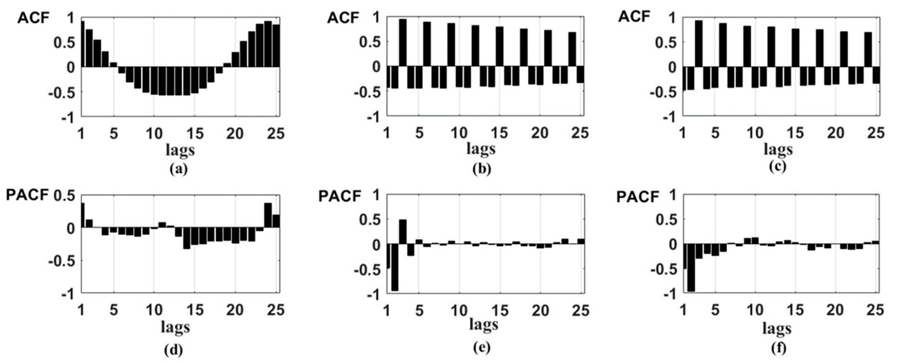
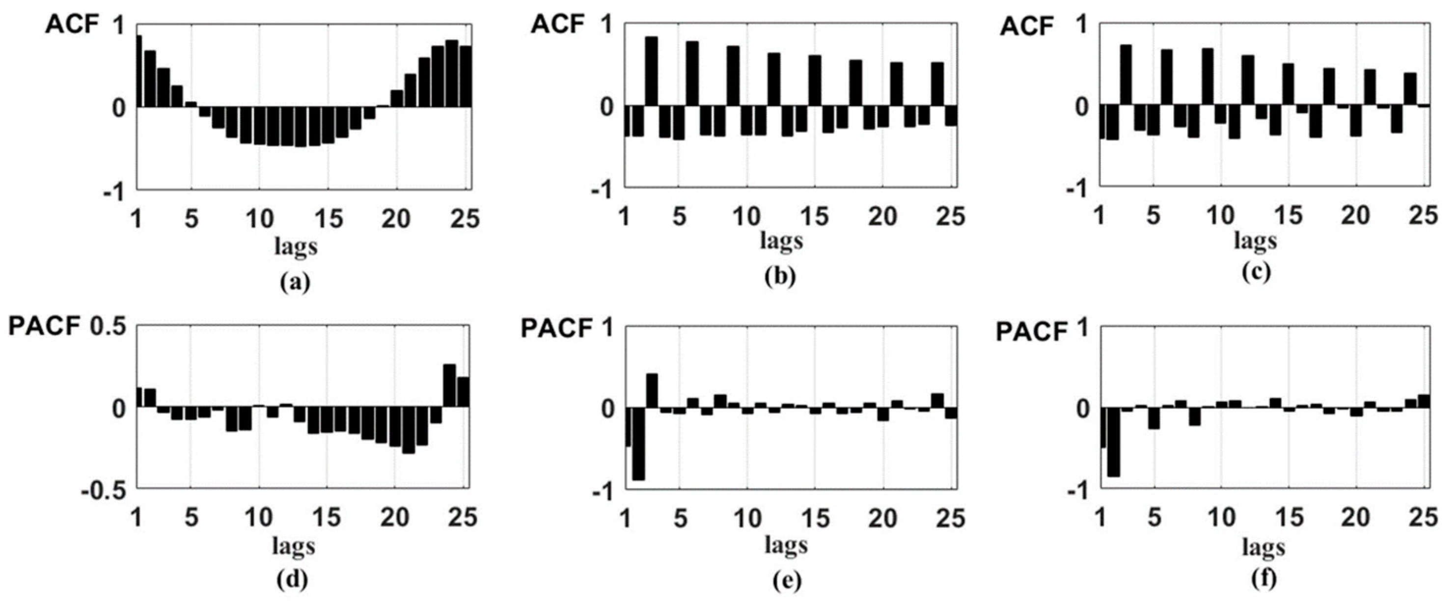
To identify HMTS regular components, we used the foF2 data recorded during the periods of absence of ionospheric anomalies. The application of Algorithm 1 showed that the components $f_{-3}$ and $g_{-3}$ are stationary (having damping ACF), thus ARIMA models can be identified for them. Figure 2 and Figure 3 show ACF and PACF of foF2 initial time series, as well as the components $f_{-3}$ and $g_{-3}$. The results confirm stationarity of the components $f_{-3}$ and $g_{-3}$. An analysis of PACF shows the possibility to identify the AR models of orders 2 and 3 for the first differences of these components. The results in Figure 2 and Figure 3 also illustrate that foF2 initial time series are non-stationary and, therefore, it is impossible to approximate them by ARIMA model without wavelet decomposition operation.

According to ratio (10) and based on the PACF of the first differences of the components $f_{-3}$ and $g_{-3}$ (Figure 3e,f), we obtain the HMTS regular component

$$A^{REG}\left(t\right)=f_{-3}(t)+g_{-3}(t)={\displaystyle \sum _k{c}_{-3,k}{\varphi }_{-3,k}(t)+}{\displaystyle \sum _k{d}_{-3,k}{\Psi }_{-3,k}(t)={\displaystyle \sum _{\mu =1,2}{\displaystyle \sum _{k=\overline{1,N^{\mu }}}{s}_{-3,k}^{\mu }{b}_{-3,k}^{\mu }}(t),}}$$

where $s_{-3,k}^{\mu }={\displaystyle \sum _{l=1}^{p^{\mu }}{\gamma }_l^{\mu }{\omega }_{-3,k-l}^{\mu }}$, $\mu =1,2$, ${\omega }_{-3,k}^1=\nabla c_{-3,k}$, ${\omega }_{-3,k}^2=\nabla d_{-3,k}$, $b_{-3,k}^1={\varphi }_{-3,k}$, $b_{-3,k}^2={\Psi }_{-3,k}$. Estimated parameters for $s_{-3,k}^1$ and $s_{-3,k}^2$ are presented in

Table 1. HMTS regular component parameters.

Period	Solar Activity	$\mathbf{Parameters} \mathbf{of} {\mathit{s}}_{\mathbf{-}\mathbf{3}\mathbf{,}\mathit{k}}^{\mathbf{1}}$			$\mathbf{Parameters} \mathbf{of} {\mathit{s}}_{\mathbf{-}\mathbf{3}\mathbf{,}\mathit{k}}^{\mathbf{2}}$
		${\gamma }_1^1$	${\gamma }_2^1$	${\gamma }_3^1$	${\gamma }_1^2$	${\gamma }_2^2$
winter	low and high	−0.6	−0.6	0.4	−0.9	−0.9
summer	low	−0.8	−0.7	−	−0.9	−0.9
	high	−0.5	−0.6	−	−0.9	−0.8

. The parameters were estimated separately for different seasons and different levels of solar activity.

Based on the data from Table 1 we obtain

(1)

for wintertime:

$s_{-3,k}^1=-0.6{\omega }_{-3,k-1}^1-0.6{\omega }_{-3,k-2}^1+0.4{\omega }_{-3,k-3}^1+a_{-3,k}^1,$

$s_{-3,k}^2=-0.9{\omega }_{-3,k-1}^2-0.9{\omega }_{-3,k-2}^2+a_{-3,k}^2,$

(2)

for summertime and high solar activity:

$s_{-3,k}^1=-0.5{\omega }_{-3,k-1}^1-0.6{\omega }_{-3,k-2}^1+a_{-3,k}^1,$

$s_{-3,k}^2=-0.9{\omega }_{-3,k-1}^2-0.8{\omega }_{-3,k-2}^2+a_{-3,k}^2,$

(3)

for summertime and low solar activity:

$s_{-3,k}^1=-0.8{\omega }_{-3,k-1}^1-0.7{\omega }_{-3,k-2}^1+a_{-3,k}^1,$

$s_{-3,k}^2=-0.9{\omega }_{-3,k-1}^2-0.9{\omega }_{-3,k-2}^2+a_{-3,k}^2.$

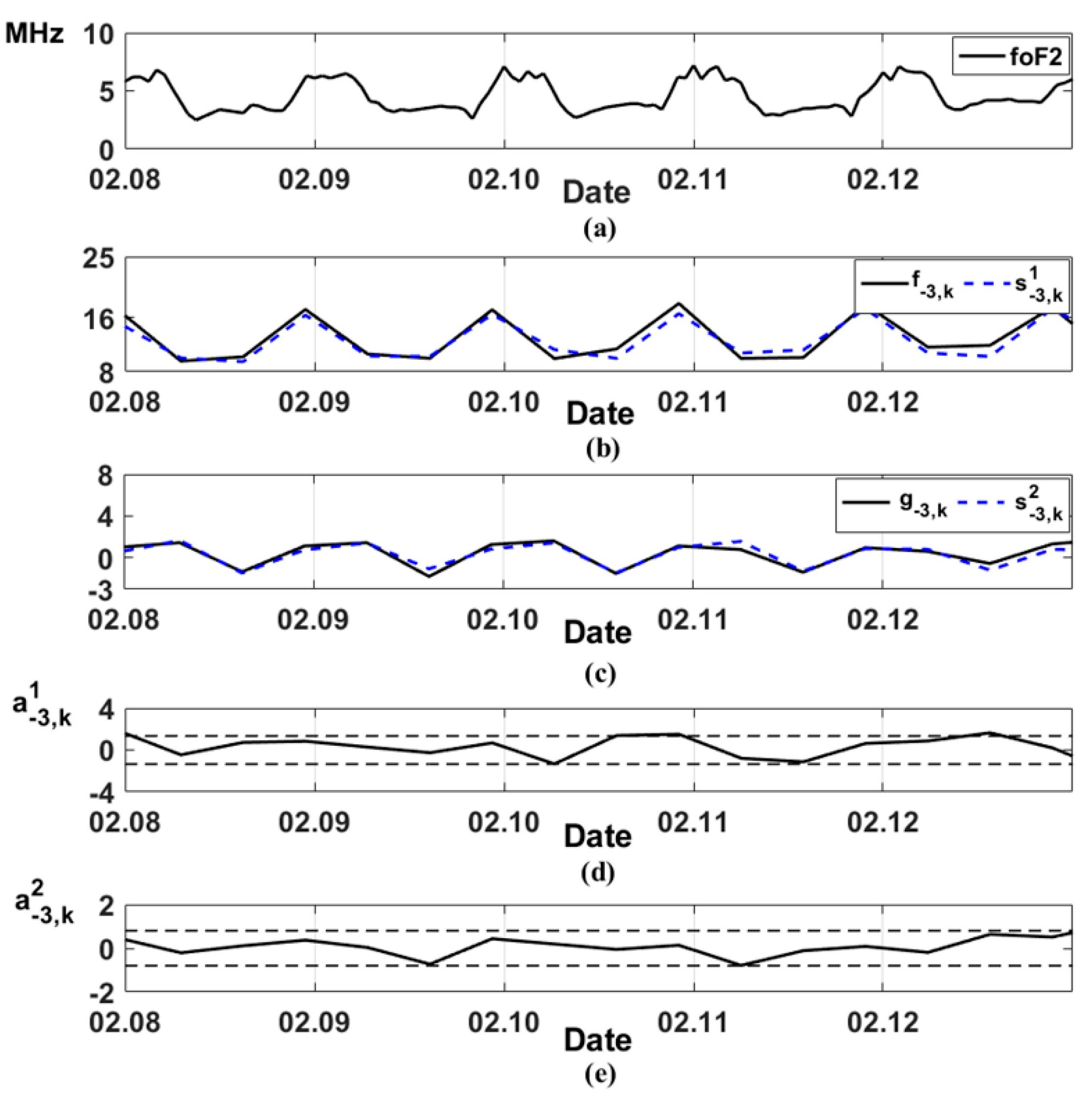
Figure 4 shows the modeling results for HMTS regular components ($f_{-3}$ and $g_{-3}$) during the absence of ionospheric anomalies. The model errors do not exceed the confidence interval that indicates their adequacy.

Table 2. Cumulative fitting criterion for the winter season.

Periods	$\mathit{Y}$ $\mathbf{for} {\mathit{s}}_{\mathbf{-}\mathbf{3}}^{\mathbf{1}}$	$\mathbf{Table} \mathbf{Value} {\mathit{\chi }}_{\mathbf{0.1}}{}^{\mathbf{2}}\mathbf{/}{\mathit{\chi }}_{\mathbf{0.05}}{}^{\mathbf{2}}$	$\mathit{Y}$ $\mathbf{for} {\mathit{s}}_{\mathbf{-}\mathbf{3}}^{\mathbf{2}}$	$\mathbf{Table} \mathbf{Value} {\mathit{\chi }}_{\mathbf{0.1}}{}^{\mathbf{2}}\mathbf{/}{\mathit{\chi }}_{\mathbf{0.05}}{}^{\mathbf{2}}$
12.15.1970–12.29.1970	18.36	24.8/27.6	28.44	26.0/28.9
02.07.2002–02.25.2002	22.08		26.40
01.30.2012–02.11.2012	16.20		13.50
02.04.2013–02.18.2013	25.90		23.76
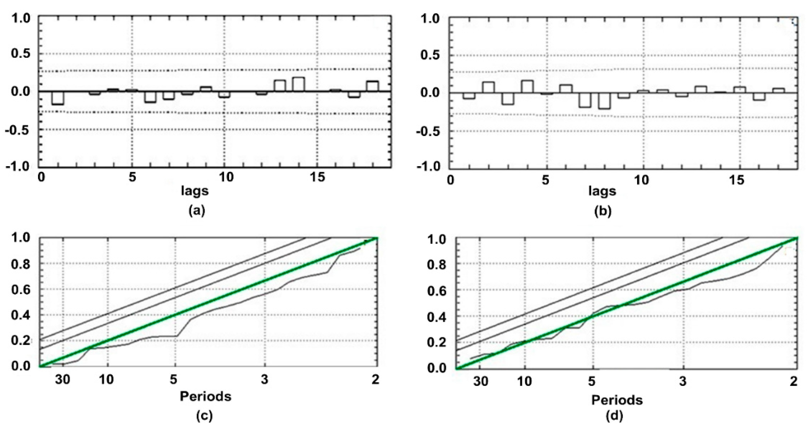
02.19.2016–03.05.2016	19.50		21.06

and

Table 3. Cumulative fitting criterion for the summer season.

Periods	$\mathit{Y}$ $\mathbf{for} {\mathit{s}}_{\mathbf{-}\mathbf{3}}^{\mathbf{1}}$	$\mathbf{Table} \mathbf{Value} {\mathit{\chi }}_{\mathbf{0.1}}{}^{\mathbf{2}}\mathbf{/}{\mathit{\chi }}_{\mathbf{0.05}}{}^{\mathbf{2}}$	$\mathit{Y}$ $\mathbf{for} {\mathit{s}}_{\mathbf{-}\mathbf{3}}^{\mathbf{2}}$	$\mathbf{Table} \mathbf{Value} {\mathit{\chi }}_{\mathbf{0.1}}{}^{\mathbf{2}}\mathbf{/}{\mathit{\chi }}_{\mathbf{0.05}}{}^{\mathbf{2}}$
06.03.1971–06.22.1971	27.26	26.0/28.9	17.39	26.0/28.9
07.11.1990–07.27.1990	16.92		18.33
08.03.2002–08.17.2002	24.84		23.76
06.15.2016–06.27.2016	20.70		21.90

, and Figure 5 show the results of validation tests for the obtained models. The tests were carried out for the foF2 data that were not used at the stage of model identification. In order to verify the models, we used the cumulative fitting criterion (Table 2 and Table 3), analysis of model residual error ACF (Figure 5a,b) and normalized cumulative periodogram (Figure 5c,d).

Based on the cumulative fitting criterion [20], the fitted model is satisfactory if

$$Y=n{\displaystyle \sum _{z=1}^Z{y}_z^2(a)}$$

is distributed approximately as ${\chi }^2(Z-p-h)$, where $Z$ are the considered first autocorrelations of model errors, $p$ is the AR model order, $h$ is the MA model order, $y_z\left(a\right)$ are the autocorrelations of model error series, $n=N-\nu$, $N$ is the series length, $\nu$ is the model difference order.

According to the criterion, if the model is inadequate, the average $Y$ grows. Consequently, the model adequacy can be verified by comparing $Y$ with the table of ${\chi }^2$ distribution. The results in Table 2 and Table 3 show that the $Y$ values of the estimated models, at a significance level $\alpha =0.05$, do not exceed the table ${\chi }^2$ values. The model adequacy is also confirmed by the analysis of residual error ACF (Figure 5a,b) and the normalized cumulative periodogram (Figure 5c,d).

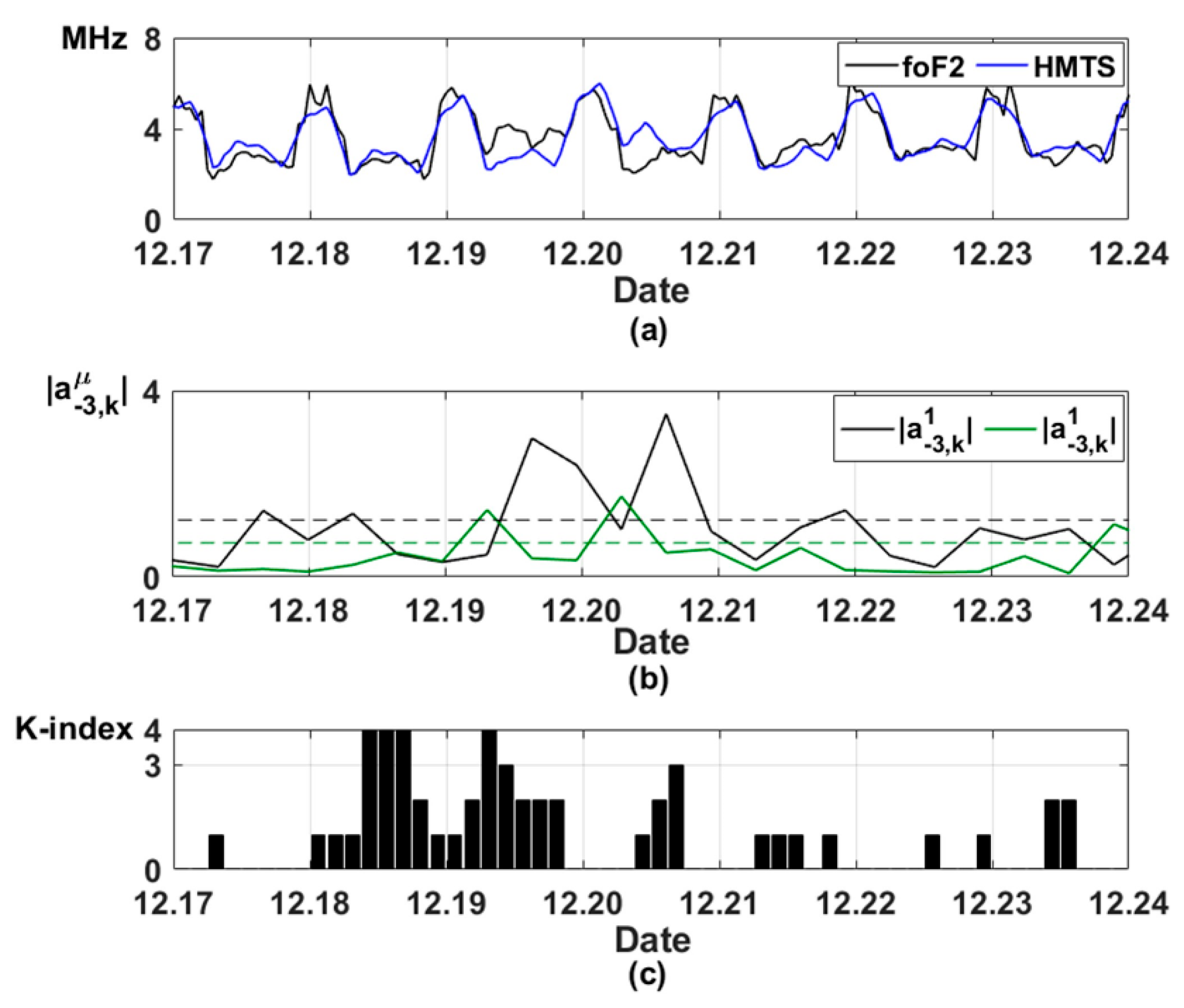
Figure 6a,b shows the results of modeling of the hourly foF2 data during the magnetic storm on 18 and 19 December 2019. Figure 6c shows the geomagnetic activity index K (K-index), which characterizes geomagnetic disturbance intensity. The K-index represents the values from 0 to 9, estimated for the three-hour interval. It is known that during increased geomagnetic activity (K > 3), anomalous changes are observed in ionospheric parameters [43]. The analysis of the results in Figure 6 shows an increase in the model errors during the increase in K-index and magnetic storm occurrence (Figure 6b). This indicates ionospheric anomaly occurrences. The results show that the HMTS allows us to detect ionospheric anomalies successfully.

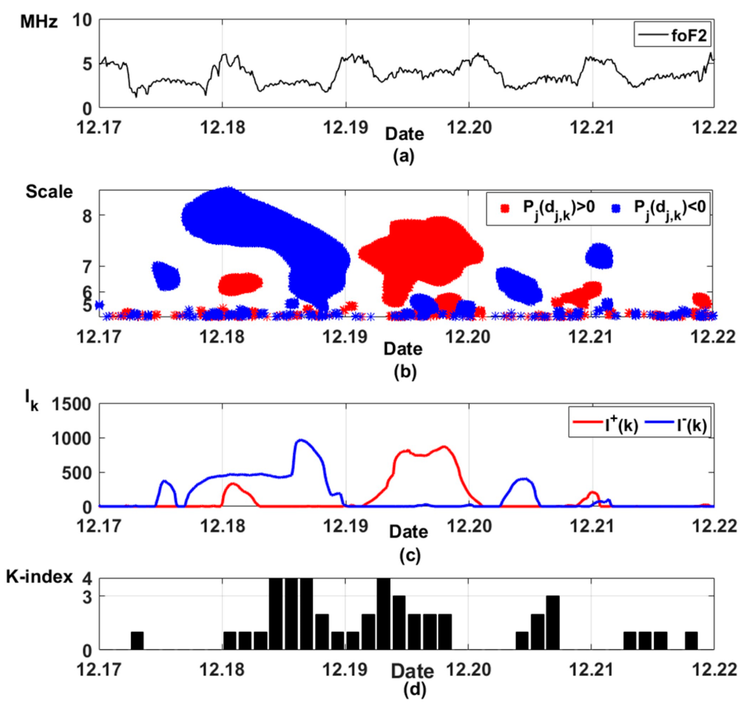
Figure 7 shows the results of the application of operation (11) to 15-min foF2 data during the same magnetic storm. Based on operation (11), ionospheric anomaly occurrences are determined by the threshold function $P_j\left(d_{j,k}\right)$ with the thresholds $T_j$.

In this paper, we used the thresholds

$$T_j=V*\sqrt{\frac{1}{\Phi -1}{\displaystyle \sum }_{k=1}^{\Phi }{\left(d_{j,k}-\overline{d_{j,k}}\right)}^2}$$

where the coefficient $V=2.3$ was estimated by minimizing a posteriori risk (ratio (15)), $\overline{d_{j,k}}$ is the average value calculated in a moving time window with the length $\Phi =480$ (it corresponds to the interval of 5 days).

Positive $(P_j\left(d_{j,k}\right)>0)$ and negative $(P_j\left(d_{j,k}\right)<0)$ anomalies were considered separately. Positive anomalies (shown in red in Figure 7b) characterize the anomalous increase in foF2 values. Negative anomalies (shown in blue in Figure 7b) characterize anomalous decrease in foF2 values. To evaluate the intensity of ionospheric anomalies we used the value

$$I_k={\displaystyle \sum }_j{P}_j\left(d_{j,k}\right)$$

Assessment of the intensity of positive $I_k^{+}$$(P_j\left(d_{j,k}\right)>0)$ and negative $I_k^{-}$$(P_j\left(d_{j,k}\right)<0)$ ionospheric anomalies is shown in Figure 7c, positive anomalies are shown in red, negative ones are shown in blue. Figure 7d shows the K-index values. The results show the occurrence of a negative ionospheric anomaly during the initial and the main phases of the magnetic storm (18 December 2019), and a positive ionospheric anomaly during the recovery phase of the storm (19 December 2019). The observed dynamics of the ionospheric parameters are characteristic of the periods of magnetic storms [43]. The results show the efficiency of HMTS application for detecting ionospheric anomalies of different intensities.

3.2. Comparison of HMTS with NARX Neural Network

To evaluate the HMTS efficiency, we compared it with the NARX neural network [44]. The NARX network is a non-linear autoregressive neural network, and it is often used to forecast time series [44,45,46,47]. The architectural structure of recurrent neural networks can take different forms. There are NARX with a Series-Parallel Architecture (NARX SPA) and NARX with a Parallel Architecture (NARX PA) [44,45].

The dynamics of the NARX SPA model is described by the equation

$$y\left(k+1\right)=F\left[x\left(k\right),x\left(k-1\right),\dots ,x\left(k-l_x\right),y\left(k\right),y\left(k-1\right),\dots ,y\left(k-l_y\right)\right],$$

where $F(\cdot )$ is the neural network display function, $y\left(k+1\right)$ is the neural network output, $x\left(k\right),x\left(k-1\right),\dots ,x\left(k-l_x\right)$ are neural network inputs, $y\left(k\right),y\left(k-1\right),\dots ,y\left(k-l_y\right)$ are past values of the time series.

In NARX PA, the network input takes the network outputs ${\widehat{y}}_i=\widehat{y}(i)$ instead of the past values of the time series $\hspace{0.17em}{y}_i=y(i),\hspace{0.17em}i=\overline{k,k-l_y}$.

The neural networks were trained separately for different seasons and different levels of solar activity. During the training, we used the data for the periods without ionospheric anomalies. We obtained the networks with delays $l_x=l_y=2$ and $l_x=l_y=5$ for each season. The results of the networks are shown in Figure 8.

Table 4. Standard deviations of neural network errors.

	SD of NARX SPA		SD of NARX PA
Season	Delays: ${\mathit{l}}_{\mathit{x}}={\mathit{l}}_{\mathit{y}}=2$	Delays: ${\mathit{l}}_{\mathit{x}}={\mathit{l}}_{\mathit{y}}=5$	Delays: ${\mathit{l}}_{\mathit{x}}={\mathit{l}}_{\mathit{y}}=2$	Delays: ${\mathit{l}}_{\mathit{x}}={\mathit{l}}_{\mathit{y}}=5$
Winter (low solar activity)	0.48	0.43	0.57	0.49
Summer (low solar activity)	0.41	0.36	0.46	0.39
Winter (high solar activity)	0.49	0.48	0.78	0.74
Summer (high solar activity)	0.42	0.36	0.45	0.36

shows the standard deviations of errors (SD) of networks, which were determined as

$$S=\sqrt{\frac{1}{n}{\displaystyle \sum _{i=1}^n{\left(y_i-{\widehat{y}}_i\right)}^2}}.$$

The analysis of the results (Figure 8, Table 4) shows that the NARX SPA predicts the data with fewer errors than the NARX PA. Sending the past time series values to the NARX SPA network input (rather than network outputs) made it possible to obtain a more accurate data prediction. The comparison results of the NARX SPA with the HMTS are presented below.

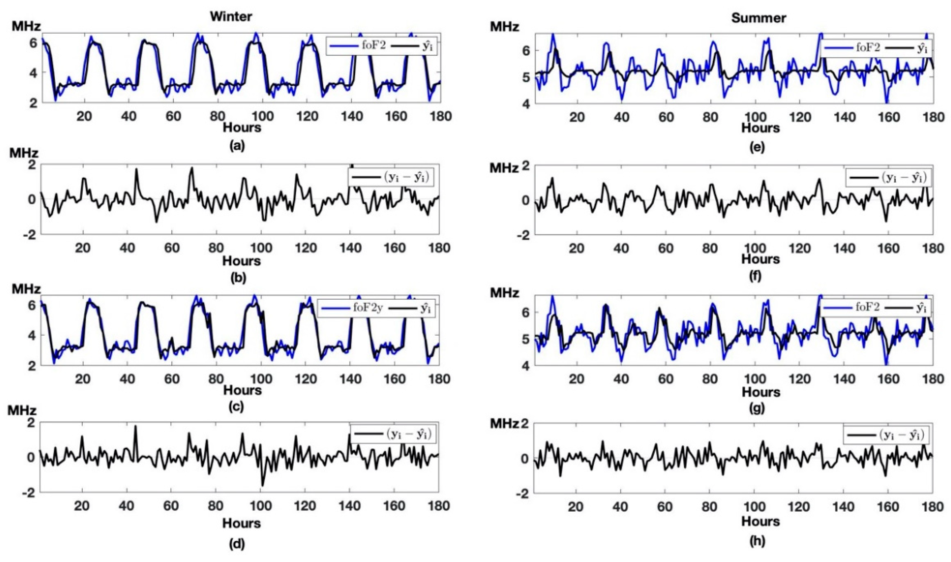
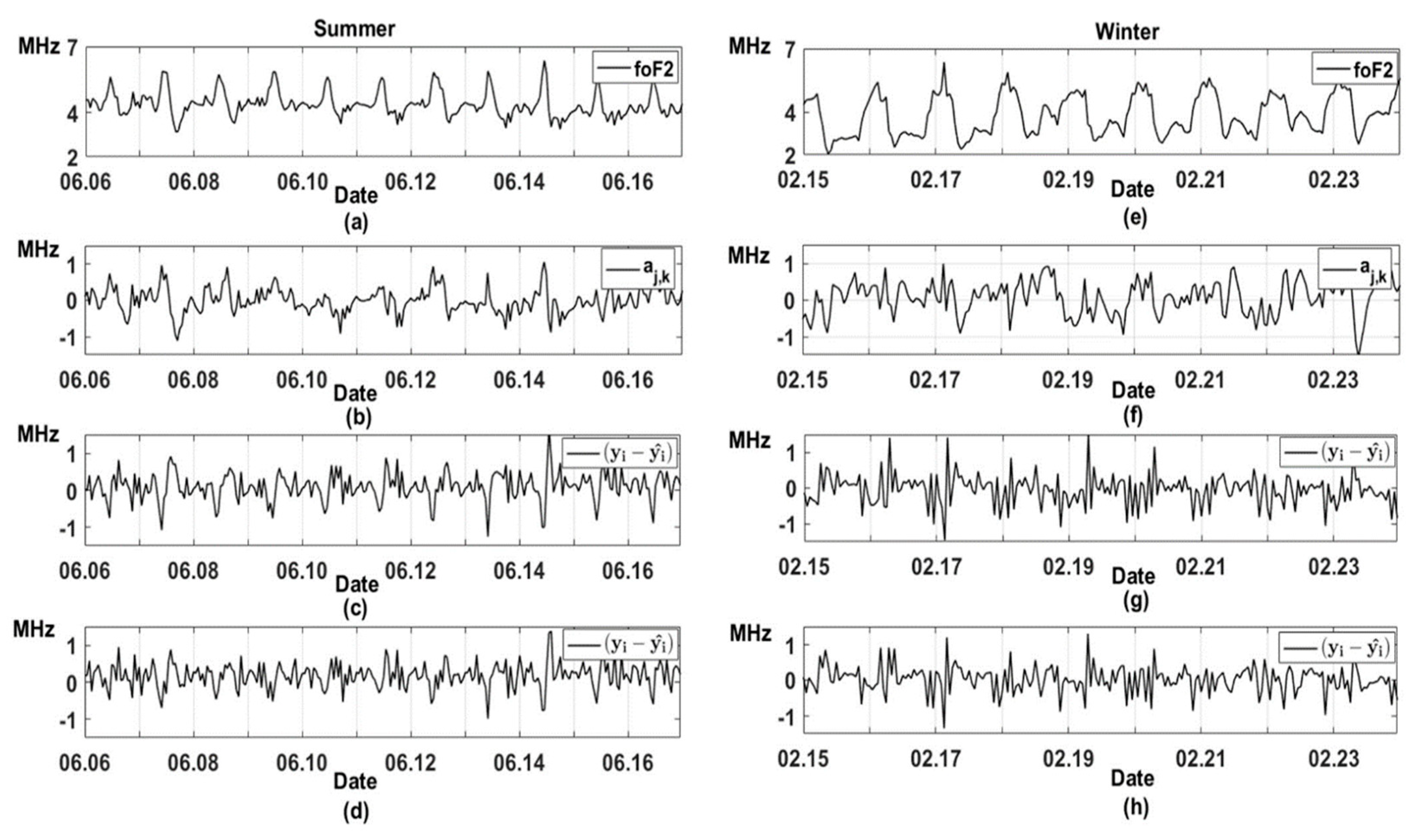
Figure 9 shows the results of ionospheric data modeling based on HMTS and NARX SPA during the periods of absence of ionospheric anomalies. The results show that the model errors have similar values for the winter and summer seasons, and vary within the interval of [−1,1], both for HMTS and NARX SPA.

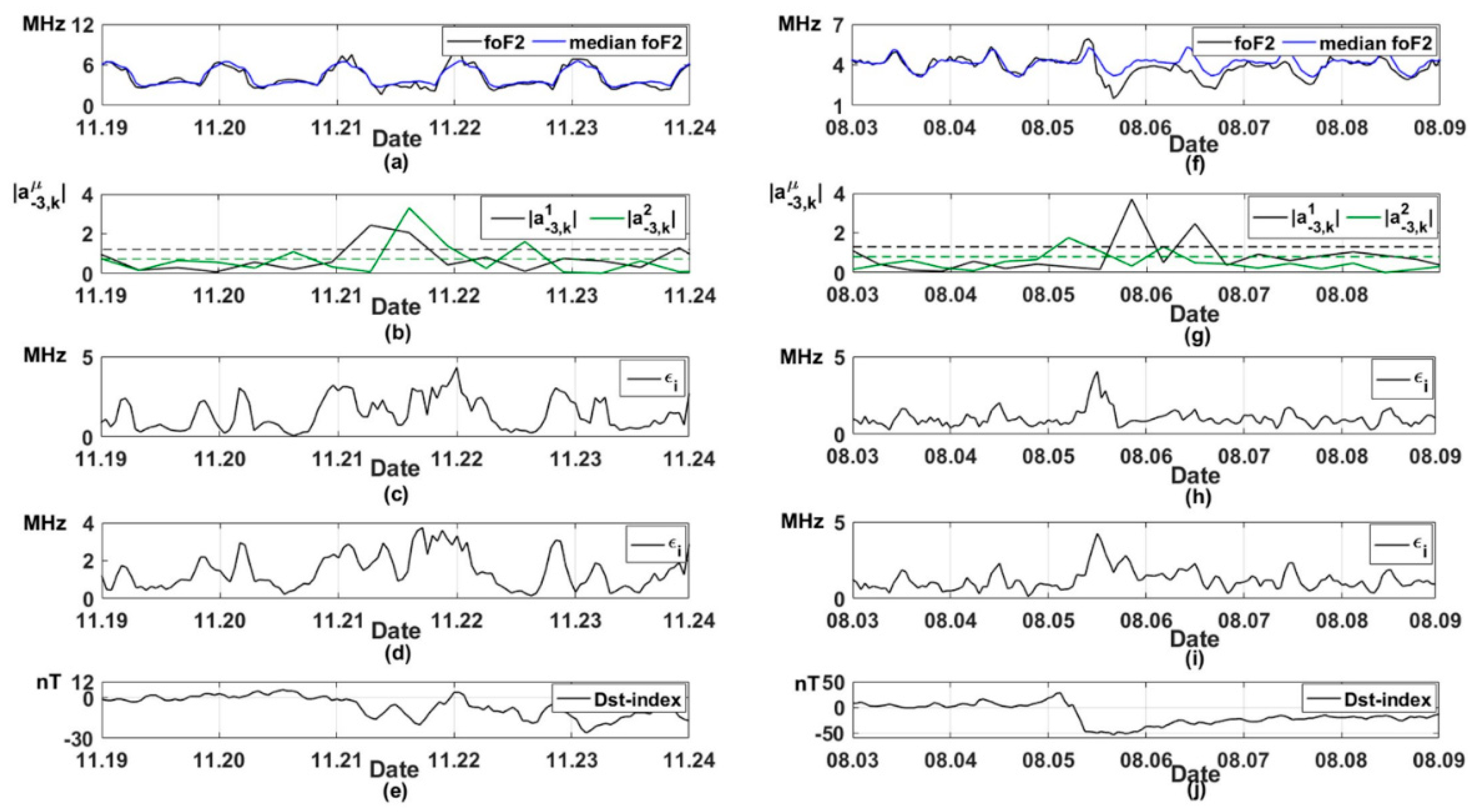
Figure 10 shows the results of the application of HMTS and NARX SPA for hourly foF2 data during magnetic storms that occurred on 21–22 November 2017 and 5–6 August 2019. NARX SPA errors were calculated in a 3-h moving time window: ${\epsilon }_i={\displaystyle {\displaystyle \sum }_{i=i-1}^{i+1}}\left|y_i-{\widehat{y}}_i\right|$. Figure 10e,j shows the geomagnetic activity Dst-index, which characterizes geomagnetic disturbance intensity during magnetic storms. Dst-index takes negative values during magnetic storms. The increases in HMTS and NARX SPA errors during the analyzed magnetic storms (Figure 10b–d,g–i) indicate ionospheric anomaly occurrences. The results show that HMTS and NARX SPA allow us to detect ionospheric anomalies successfully. However, an increase in NARX SPA errors is also observed in wintertime on the eve and after the magnetic storm (Figure 10c,d). This shows the presence of false alarms.

The results of detecting ionospheric anomalies based on HMTS and NARX SPA are shown in

Table 5. Results for wintertime and high solar activity.

HMTS			NARX SPA
Signal/Noise	Detected/False		Detected/False
	$\mathbf{Component} {\mathit{f}}_{-3}$	$\mathbf{Component} {\mathit{g}}_{-3}$	Delays: ${\mathit{l}}_{\mathit{x}}={\mathit{l}}_{\mathit{y}}=2$	Delays: ${\mathit{l}}_{\mathit{x}}={\mathit{l}}_{\mathit{y}}=5$
1.3	95%/0%	78%/2%	86%/5%	96%/4%
1	92%/0%	74%/7%	76%/8%	94%/9%
0.8	85%/3%	74%/11%	75%/12%	84%/12%

,

Table 6. Results for wintertime and low solar activity.

HMTS			NARX SPA
Signal/Noise	Detected/False		Detected/False
	$\mathbf{Component} {\mathit{f}}_{-3}$	$\mathbf{Component} {\mathit{g}}_{-3}$	Delays: ${\mathit{l}}_{\mathit{x}}={\mathit{l}}_{\mathit{y}}=2$	Delays: ${\mathit{l}}_{\mathit{x}}={\mathit{l}}_{\mathit{y}}=5$
1.3	97%/0%	90%/5%	81%/1%	89%/2%
1	96%/2%	89%/12%	73%/12%	84%/12%
0.8	85%/6%	89%/17%	70%/19%	82%/18%

,

Table 7. Results for summertime and high solar activity.

HMTS			NARX SPA
Signal/Noise	Detected/False		Detected/False
	$\mathbf{Component} {\mathit{f}}_{-3}$	$\mathbf{Component} {\mathit{g}}_{-3}$	Delays: ${\mathit{l}}_{\mathit{x}}={\mathit{l}}_{\mathit{y}}=2$	Delays: ${\mathit{l}}_{\mathit{x}}={\mathit{l}}_{\mathit{y}}=5$
1.3	79%/0%	80%/2%	79%/5%	81%/7%
1	70%/0%	65%/4%	71%/15%	72%/14%
0.8	55%/1%	63%/10%	64%/18%	64%/17%

and

Table 8. Results for summertime and low solar activity.

HMTS			NARX SPA
Signal/Noise	Detected/False		Detected/False
	$\mathbf{Component} {\mathit{f}}_{-3}$	$\mathbf{Component} {\mathit{g}}_{-3}$	Delays: ${\mathit{l}}_{\mathit{x}}={\mathit{l}}_{\mathit{y}}=2$	Delays: ${\mathit{l}}_{\mathit{x}}={\mathit{l}}_{\mathit{y}}=5$
1.3	94%/0%	83%/3%	92%/2%	93%/3%
1	90%/0%	80%/9%	90%/6%	91%/9%
0.8	86%/2%	80%/13%	85%/11%	84%/15%

. The estimates were based on statistical modeling. The HMTS results are shown for the 90% confidence interval. The analysis of the results shows that NARX SPA efficiency exceeds that for HMTS during high solar activity. However, the frequency of false alarms for HMTS is significantly less than that for NARX SPA.

4. Conclusions

The paper proposes a hybrid model of time series of complex structure. The model is based on the combination of function expansions in a wavelet series with ARIMA models. Ionospheric critical frequency data were used to estimate the HMTS efficiency. The estimates showed:

1.

The HMTS regular component adequately describes ionospheric parameter time series during the periods without ionospheric anomalies. Application of wavelet decomposition allows us to detect regular components of ionospheric parameter time series and to use the ARIMA model;

2.

Analysis of HMTS regular component errors allows us to detect ionospheric anomalies during a magnetic storm;

3.

The HMTS anomalous component allows us to detect ionospheric anomalies of different intensities by threshold functions.

Comparison of HMTS with NARX with Series-Parallel Architecture confirmed the HMTS efficiency to detect anomalies in the ionospheric critical frequency data. The results of the experiments showed that the efficiency of the NARX neural network slightly exceeds that of HMTS (about 2–3%) during high solar activity. However, the frequency of false alarms in NARX is significantly higher (about 15%). During the periods of low solar activity, the efficiency of HMTS exceeds that of NARX.

The HMTS can be used for modeling and analysis of time series of complex structure, including seasonal components and local features of various forms.

References

1. Song, R.; Zhang, X.; Zhou, C.; Liu, J.; He, J. Predicting TEC in China based on the neural networks optimized by genetic algorithm. Adv. Space Res. 2018, 62, 745–759. [Google Scholar] [CrossRef]
2. Bailey, R.L.; Leonhardt, R. Automated detection of geomagnetic storms with heightened risk of GIC. Earth Planets Space 2016, 68, 99. [Google Scholar] [CrossRef]
3. Mandrikova, O.V.; Solovev, I.S.; Zalyaev, T.L. Methods of analysis of geomagnetic field variations and cosmic ray data. Earth Planets Space 2014, 66, 148. [Google Scholar] [CrossRef] [Green Version]
4. Tang, R.; Zeng, F.; Chen, Z.; Wang, J.-S.; Huang, C.-M.; Wu, Z. The Comparison of Predicting Storm-Time Ionospheric TEC by Three Methods: ARIMA, LSTM, and Seq2Seq. Atmosphere 2020, 11, 316. [Google Scholar] [CrossRef] [Green Version]
5. Perol, T.; Gharbi, M.; Denolle, M. Convolutional neural network for earthquake detection and location. Sci. Adv. 2018, 4, e1700578. [Google Scholar] [CrossRef] [Green Version]
6. Tronin, A.A. Satellite Remote Sensing in Seismology. A Review. Remote Sens. 2009, 2, 124–150. [Google Scholar] [CrossRef] [Green Version]
7. Chierici, F.; Embriaco, D.; Pignagnoli, L. A new real-time tsunami detection algorithm. J. Geophys. Res. Ocean. 2017, 122, 636–652. [Google Scholar] [CrossRef]
8. Kim, S.-K.; Lee, E.; Park, J.; Shin, S. Feasibility Analysis of GNSS-Reflectometry for Monitoring Coastal Hazards. Remote Sens. 2021, 13, 976. [Google Scholar] [CrossRef]
9. Alperovich, L.; Eppelbaum, L.; Zheludev, V.; Dumoulin, J.; Soldovieri, F.; Proto, M.; Bavusi, M.; Loperte, A. A new combined wavelet methodology: Implementation to GPR and ERT data obtained in the Montagnole experiment. J. Geophys. Eng. 2013, 10, 25017. [Google Scholar] [CrossRef]
10. Amigó, J.M.; Small, M. Mathematical methods in medicine: Neuroscience, cardiology and pathology. Philos. Trans. R. Soc. A Math. Phys. Eng. Sci. 2017, 375. [Google Scholar] [CrossRef] [Green Version]
11. Chen, J.; Heincke, B.; Jegen, M.; Moorkamp, M. Using empirical mode decomposition to process marine magnetotelluric data. Geophys. J. Int. 2012, 190, 293–309. [Google Scholar] [CrossRef] [Green Version]
12. Chen, L.; Han, W.; Huang, Y.; Cao, X. Online Fault Diagnosis for Photovoltaic Modules Based on Probabilistic Neural Network. Eur. J. Electr. Eng. 2019, 21, 317–325. [Google Scholar] [CrossRef]
13. Robbins, H.; Monro, S. A Stochastic Approximation Method. Ann. Math. Stat. 1951, 22, 400–407. [Google Scholar] [CrossRef]
14. Vasconcelos, J.C.S.; Cordeiro, G.M.; Ortega, E.M.M.; De Rezende, É.M. A new regression model for bimodal data and applications in agriculture. J. Appl. Stat. 2021, 48, 349–372. [Google Scholar] [CrossRef]
15. Valipour, M.; Banihabib, M.E.; Behbahani, S.M.R. Comparison of the ARMA, ARIMA, and the autoregressive artificial neural network models in forecasting the monthly inflow of Dez dam reservoir. J. Hydrol. 2013, 476, 433–441. [Google Scholar] [CrossRef]
16. Li, S.; Wang, Q. India’s dependence on foreign oil will exceed 90% around 2025—The forecasting results based on two hybridized NMGM-ARIMA and NMGM-BP models. J. Clean. Prod. 2019, 232, 137–153. [Google Scholar] [CrossRef]
17. Wu, X.; Zhou, J.; Yu, H.; Liu, D.; Xie, K.; Chen, Y.; Hu, J.; Sun, H.; Xing, F. The Development of a Hybrid Wavelet-ARIMA-LSTM Model for Precipitation Amounts and Drought Analysis. Atmosphere 2021, 12, 74. [Google Scholar] [CrossRef]
18. Miljkovic, D.; Shaik, S.; Miranda, S.; Barabanov, N.; Liogier, A. Globalisation and Obesity. World Econ. 2015, 38, 1278–1294. [Google Scholar] [CrossRef]
19. Ivanov, L.; Collins, C.; Margolina, T. Reconstruction of Diffusion Coefficients and Power Exponents from Single Lagrangian Trajectories. Fluids 2021, 6, 111. [Google Scholar] [CrossRef]
20. Box, G.E.P.; Jenkins, G.M. Time Series Analysis: Forecasting and Control, Rev. ed.; Holden-Day Series in Time Series Analysis and Digital Processing; Holden-Day: San Francisco, CA, USA, 1976; ISBN 978-0-8162-1104-3. [Google Scholar]
21. Liu, J.; Kumar, S.; Palomar, D.P. Parameter Estimation of Heavy-Tailed AR Model with Missing Data via Stochastic EM. IEEE Trans. Signal Process. 2019, 67, 2159–2172. [Google Scholar] [CrossRef] [Green Version]
22. Chatfield, C.; Koehler, A.B.; Ord, J.K.; Snyder, R.D. A New Look at Models for Exponential Smoothing. J. R. Stat. Soc. Ser. D 2001, 50, 147–159. [Google Scholar] [CrossRef]
23. Estévez, J.; Bellido-Jiménez, J.A.; Liu, X.; García-Marín, A.P. Monthly Precipitation Forecasts Using Wavelet Neural Networks Models in a Semiarid Environment. Water 2020, 12, 1909. [Google Scholar] [CrossRef]
24. Mbatha, N.; Bencherif, H. Time Series Analysis and Forecasting Using a Novel Hybrid LSTM Data-Driven Model Based on Empirical Wavelet Transform Applied to Total Column of Ozone at Buenos Aires, Argentina (1966–2017). Atmosphere 2020, 11, 457. [Google Scholar] [CrossRef]
25. Mehdizadeh, S.; Fathian, F.; Adamowski, J.F. Hybrid artificial intelligence-time series models for monthly streamflow modeling. Appl. Soft Comput. 2019, 80, 873–887. [Google Scholar] [CrossRef]
26. Shishegaran, A.; Saeedi, M.; Kumar, A.; Ghiasinejad, H. Prediction of air quality in Tehran by developing the nonlinear ensemble model. J. Clean. Prod. 2020, 259, 120825. [Google Scholar] [CrossRef]
27. Büyükşahin, Ü.Ç.; Ertekin, Ş. Improving forecasting accuracy of time series data using a new ARIMA-ANN hybrid method and empirical mode decomposition. Neurocomputing 2019, 361, 151–163. [Google Scholar] [CrossRef] [Green Version]
28. Vivas, E.; Allende-Cid, H.; Salas, R.; Bravo, L. Polynomial and Wavelet-Type Transfer Function Models to Improve Fisheries’ Landing Forecasting with Exogenous Variables. Entropy 2019, 21, 1082. [Google Scholar] [CrossRef] [Green Version]
29. Sebastian, D.E.; Ganguly, S.; Krishnaswamy, J.; Duffy, K.; Nemani, R.; Ghosh, S. Multi-Scale Association between Vegetation Growth and Climate in India: A Wavelet Analysis Approach. Remote Sens. 2019, 11, 2703. [Google Scholar] [CrossRef] [Green Version]
30. Hurat, B.; Alvarado, Z.; Gilles, J. The Empirical Watershed Wavelet. J. Imaging 2020, 6, 140. [Google Scholar] [CrossRef]
31. Casado-Vara, R.; del Rey, A.M.; Pérez-Palau, D.; De-La-Fuente-Valentín, L.; Corchado, J. Web Traffic Time Series Forecasting Using LSTM Neural Networks with Distributed Asynchronous Training. Mathematics 2021, 9, 421. [Google Scholar] [CrossRef]
32. Moon, J.; Hossain, B.; Chon, K.H. AR and ARMA model order selection for time-series modeling with ImageNet classification. Signal Process. 2021, 183, 108026. [Google Scholar] [CrossRef]
33. Yang, S.; Chen, H.-C.; Wu, C.-H.; Wu, M.-N.; Yang, C.-H. Forecasting of the Prevalence of Dementia Using the LSTM Neural Network in Taiwan. Mathematics 2021, 9, 488. [Google Scholar] [CrossRef]
34. Phan, T.-T.-H.; Nguyen, X.H. Combining statistical machine learning models with ARIMA for water level forecasting: The case of the Red River. Adv. Water Resour. 2020, 142, 103656. [Google Scholar] [CrossRef]
35. Khan, M.H.; Muhammad, N.S.; El-Shafie, A. Wavelet based hybrid ANN-ARIMA models for meteorological drought forecasting. J. Hydrol. 2020, 590, 125380. [Google Scholar] [CrossRef]
36. Chui, C.K. An Introduction to Wavelets; Wavelet Analysis and Its Applications; Academic Press: Boston, MA, USA, 1992; ISBN 978-0-12-174584-4. [Google Scholar]
37. Mallat, S.G. A Wavelet Tour of Signal Processing; Academic Press: San Diego, CA, USA, 1999; ISBN 978-0-12-466606-1. [Google Scholar]
38. Daubechies, I. Ten Lectures on Wavelets; CBMS-NSF Regional Conference Series in Applied Mathematics; Society for Industrial and Applied Mathematics: Philadelphia, PA, USA, 1992; ISBN 978-0-89871-274-2. [Google Scholar]
39. Jaffard, S. Pointwise smoothness, two-microlocalization and wavelet coefficients. Publ. Matemàtiques 1991, 35, 155–168. [Google Scholar] [CrossRef] [Green Version]
40. Berger, J.O. Statistical Decision Theory and Bayesian Analysis, 2nd ed.; Springer Series in Statistics; Springer: New York, NY, USA, 1993; ISBN 978-0-387-96098-2. [Google Scholar]
41. Hernández-Pajares, M.; Juan, J.M.; Sanz, J.; Aragón-Àngel, À.; García-Rigo, A.; Salazar, D.; Escudero, M. The ionosphere: Effects, GPS modeling and the benefits for space geodetic techniques. J. Geod. 2011, 85, 887–907. [Google Scholar] [CrossRef]
42. Ferreira, A.A.; Borries, C.; Xiong, C.; Borges, R.A.; Mielich, J.; Kouba, D. Identification of potential precursors for the occurrence of Large-Scale Traveling Ionospheric Disturbances in a case study during September 2017. J. Space Weather Space Clim. 2020, 10, 32. [Google Scholar] [CrossRef]
43. Danilov, A. Ionospheric F-region response to geomagnetic disturbances. Adv. Space Res. 2013, 52, 343–366. [Google Scholar] [CrossRef]
44. Diaconescu, E. The use of NARX neural networks to predict chaotic time series. WSEAS Trans. Comp. Res. 2008, 3, 182–191. [Google Scholar]
45. Narendra, K.; Parthasarathy, K. Identification and control of dynamical systems using neural networks. IEEE Trans. Neural Netw. 1990, 1, 4–27. [Google Scholar] [CrossRef] [Green Version]
46. Ma, Q.; Liu, S.; Fan, X.; Chai, C.; Wang, Y.; Yang, K. A Time Series Prediction Model of Foundation Pit Deformation Based on Empirical Wavelet Transform and NARX Network. Mathematics 2020, 8, 1535. [Google Scholar] [CrossRef]
47. Boussaada, Z.; Curea, O.; Remaci, A.; Camblong, H.; Bellaaj, N.M. A Nonlinear Autoregressive Exogenous (NARX) Neural Network Model for the Prediction of the Daily Direct Solar Radiation. Energies 2018, 11, 620. [Google Scholar] [CrossRef] [Green Version]
Figure 1. AFC of the scaling function and the wavelet for m = 1 , 2 , 3 , 4 obtained for the 3rd-order Daubechies wavelet.
Mathematics 09 01122 g001
Figure 2. The analyzed period is from 4 January 2014 to 29 January 2014 (high solar activity): (a) ACF of the original signal; (b) ACF of the component f 3 ; (c) ACF of the component g 3 ; (d) PACF of the 1st difference of the original signal; (e) PACF of the 1st difference of the component f 3 ; (f) PACF of the 1st difference of the component g 3 .
Mathematics 09 01122 g002
Figure 3. The analyzed period is from 9 February 2008 to 27 February 2008 (low solar activity): (a) ACF of the original signal; (b) ACF of the component f 3 ; (c) ACF of the component g 3 ; (d) PACF of the 1st difference of the original signal; (e) PACF of the 1st difference of the component f 3 ; (f) PACF of the 1st difference of the component g 3 .
Mathematics 09 01122 g003
Figure 4. Modeling of the components f 3 and g 3 : (a) foF2 data (8 February 2011–12 February 2011); (b) component f 3 (black) and its model values s 3 , k 1 (blue dashed line); (c) component g 3 (black) and its model values s 3 , k 2 (blue dashed line); (d) errors of s 3 , k 1 ; (e) errors of s 3 , k 2 . On the graphs (d,e) the dashed lines show 70% confidence intervals.
Mathematics 09 01122 g004
Figure 5. Results of model verification: ACF of residual errors: (a) a 3 , k 1 ; (b) a 3 , k 2 ; cumulative periodogram of residual errors: (c) a 3 , k 1 ; (d) a 3 , k 2 .
Mathematics 09 01122 g005
Figure 6. Modeling of foF2 data for the period from 17 December 2019 to 24 December 2019. (a) foF2 data (black), HMTS (blue); (b) errors of s 3 , k 1 (black) and s 3 , k 2 (green), dashed lines show 70% confidence intervals; (c) K-index values.
Mathematics 09 01122 g006
Figure 7. Modeling of foF2 data for the period from 17 December 2019 to 22 December 2019. (a) 15-minute data of foF2; (b) positive (red) and negative (blue) ionospheric anomalies; (c) ionospheric anomaly intensity; (d) K-index values.
Mathematics 09 01122 g007
Figure 8. Network errors: (a,e) foF2 data (blue), NARX PA output (black); (b,f) NARX PA errors; (c,g) foF2 data (blue), NARX SPA output (black); (d,h) NARX SPA errors.
Mathematics 09 01122 g008
Figure 9. Errors of HMTS and NARX SPA for summer (from 6 June 2019 to 16 June 2019) and winter (from 15 February 2019 to 23 February 2019) seasons: (a,e) foF2 data; (b,f) HMTS errors; (c,g) NARX SPA errors (network delays l x = l y = 2 ); (d,h) NARX SPA errors (network delays l x = l y = 5 ).
Mathematics 09 01122 g009
Figure 10. Modeling of hourly foF2 data: (a,f) recorded foF2 data (black), foF2 median (blue); (b,g) errors of s 3 , k 1 (black) and s 3 , k 2 (green), dashed lines show 70% confidence intervals; (c,h) NARX SPA errors (network delays l x = l y = 2 ); (d,i) NARX SPA errors (network delays l x = l y = 5 ); (e,j) Dst-index of geomagnetic activity.
Mathematics 09 01122 g010