Time Series Forecasting for Wind Energy Systems Based on High Order Neural Networks

Abstract

Wind energy is one of the most promising alternatives as energy sources; however, to obtain the best results, producers need to forecast the wind speed, generated power and energy price in order to provide the appropriate tools for optimal operation, planning, control and marketing both for isolated wind systems and for those that are interconnected to a main distribution network. For the present work, a novel methodology is proposed for the forecasting of time series in wind energy systems; it consists of a high-order neural network that is trained on-line by the extended Kalman filter algorithm. Unlike most modern artificial intelligence methods of forecasting, which are based on hybridizations, data pre-filtering or deep learning methods, the proposed method is based on the simplicity of implementation, low computational complexity and real-time operation to produce 15-step-ahead forecasting in a time series of wind speed, generated power and energy price. The proposed scheme has been evaluated using real data from open access repositories of wind farms. The results show that an on-line training of the neural network produces high precision, without the need for any other information beyond a few past observations.

1. Introduction

Nowadays, the demand for electricity is growing rapidly as a result of social, economic and industrial development, while the reserves of fossil fuels for power generation are rapidly reducing and pollution is increasing. As a result of this contradiction, humanity is looking for renewable, clean and pollution-free energy sources [1]. Wind energy meets the above requirements despite the high cost of wind energy over that of fossil fuels. Wind energy may become an important source of energy in the near future, especially for supplying small loads at power plants in remote places where there is a rich wind energy resource making it the preferred location to extract kinetic energy from the wind [2].

Unfortunately, wind speed is considered one of the most difficult climatic parameters to model and forecast due to the complex parameter structures that strongly affect the wind, such as topographic properties of the earth, the rotation of the world, and the difference in temperature and pressure [2,3,4]. Due to the continuous increase of wind energy implementation in power systems, the problems caused by the volatile nature of wind speed and the occurrences in system operations, such as scheduling and dispatch, have drawn the attention of system operators, public services and researchers, for the development of state-of-the-art power, wind speed and price forecasting methods. These methods have the necessary ability to reduce the influence of intermittent wind energy on system operations, as well as the capability to harvest wind energy efficiently [5].

Research in wind energy is a very active area and is yielding results for generators, electrical system operators and market operators. In this sense, the rapid expansion of wind generation capacity in the last 20 years has led to advances in wind forecasting techniques, which in turn have been driven by advances in the affordability and power of computer technology. Furthermore, continuous innovations in statistics and machine learning has resulted in increased accuracy, allowing the use of more sophisticated techniques and more accurate forecasting tools. Forecasting techniques have also paid dividends, particularly for forecasting on very short and short-term timescales, to drive future developments in wind forecasting technology and current plans to greatly increase wind capacity: however, improvements are still needed in the existing forecasting models [6].

Time series forecasting in wind energy, which includes wind speed, power output and energy price, can be useful in various areas; for example, using the wind speed forecast makes it possible to optimize the maintenance planning according to periods of weak wind speed. Using power forecasting helps to optimally tune the wind turbine controller since the turbine curve provided by the manufacturer is unable to give a real value of the generated power. Turbine curve modeling can also be used to account for the amount of energy loss while the wind turbine is shut down for maintenance. Additionally, very short-term forecasting is used to plan turbine control actions, while long-term forecasting allows issues to be properly handled with regard to energy marketing and reducing financial and technical risk [7]. Wind power forecasting tools are invaluable because they allow better dispatch, scheduling, unit engagement of thermal and hydroelectric generators and energy storage plants, as well as provide a more competitive market. Therefore, if the error in forecasting wind power is reduced, electricity markets can trade with greater certainty [6]. Hence, the existence of an accurate global forecast of the time series of wind energy reduces the financial and technical risk of the uncertainty of the wind in energy production for all participants in the electricity market by integrating wind energy with easier tasks [6].

Therefore, for the wind energy market to work efficiently, it is evident that forecasting wind energy production in the near future is crucial for both isolated wind systems and interconnected wind systems. Thus, having efficient tools for the forecasting of wind energy time series helps producers make decisions for the operation, programming and marketing of wind energy systems [2,8]. To that end, research efforts have recently been directed towards the design of new combined algorithms and combination methods that exploit different single forecasting models and improve forecasting performance while providing reasonable computation time.

Most of the wind forecasting techniques can be classified into two main groups, namely, physical methods and statistical methods [5]. In summary, the first group takes into account physical considerations, such as location, wind farm design and temperature, to reach the estimate and uses the output from numerical weather forecasting models that provide weather forecasts using the mathematical model of the atmosphere. The second group aims to describe the relationship between the historical time series of wind speed (or power or price) in the place of interest by generally recursive techniques, whether statistical or based on artificial intelligence [5]. In [5,6], an in-depth analysis was performed regarding the state-of-the-art of forecasting methods for time series in wind systems. In the case of forecasting methods based on artificial intelligence, fuzzy logic, artificial neural networks, support vector machines, Bayesian networks, and genetic programming are generally adopted for time series forecasting of wind systems.

Forecasting methods based on artificial intelligence are simplified models of biological intelligence and have proven to be efficient forecasting techniques due to their capabilities, such as self-learning, easy implementation and the establishment of nonlinear relationships between input and output data sets with a high degree of precision. According to the review of forecasting approaches for wind energy and power carried out in [5], a large number of recent publications have used artificial neural networks (NN) instead of conventional statistical models, as they are based on linear assumptions and are therefore deficient in the adequate modeling of the nonlinearity of the relationship. On the other hand, artificial intelligence methods, mainly artificial NN, learn from experience, using data, which is called a data-driven approach. Among these, we can mention [9], where a 6 h wind speed forecast was made, equivalent to six steps forward with the linear autoregressive–moving average model. In addition, wavelets pre-filtering was previously carried out in the data set to obtain better results. Similarly, in [10], the forecasting was carried out using wavelet theory to filter the low-frequency parts of the whole wind speed and then the autoregressive–moving average model was used to forecast the wind speed of filtered data. The data set corresponds to a total of 120 points, where each sample point was taken every hour and 90 samples were used for training. The remaining 30 points were for the forecasting test.

As previously mentioned, NNs are a promising approach for forecasting wind energy, power and price because they present better results than other techniques [6]. Among the works that use NNs, we can name the one presented in [2], where an empirical mode decomposition-based multilayer feed-forward neural network was used to perform the wind speed forecast, which uses two types of data: mean monthly wind speed and mean daily wind speed. For the first case, up to 36 observations were used to train the network, and forecasting of up to 12 samples were made with this technique. For the second case, 113 observations were used as the training set and 10 samples were forecasted. Using a nonlinear autoregressive neural network, the wind speed of a 5-day horizon was forecasted, and energy production was estimated. The data used were 4320 samples for training and 720 for testing [7]. Aqsa et al. proposed a deep neural network both as a base-regressor and as a meta-regression with 24 time series delays. In that work, a wind power and wind speed dataset was used, where 90% of the data was used for training and only 10% for testing [11]. In the work presented by Erasmo et al., good results were achieved for forecasting the wind speed by implementing a multilayer neural network, where it proposes an architecture of two hidden layers; in addition, the iterative strategy was used to forecast up to three steps forward with two delays as the input [12]. Two different wind speed time series are used in [13], and a hybrid model based on the empirical mode decomposition and an NN is implemented. It also considers four time series delays as input to the neural network, and as a result, a forecasting of one, two and three steps forward of wind speed is obtained. Gong Li et al. [14] present a robust two-step methodology for wind speed forecasting based on a Bayesian combination algorithm, and three types of feed-forward NNs, i.e., an adaptive linear element network, backpropagation network, and radial basis function network. All NNs receive eight past observations as inputs. Another work where data are pre-filtered to forecast wind speed is presented in [15], which uses a backpropagation neural network with a Levenberg–Marquardt algorithm. The wind speed data are filtered into two components, i.e., low-frequency and several high-frequencies, by the wavelet decomposition method. Then, the NN forecasts every component, and the forecasting components are reconstructed to obtain the forecast of wind speed. A total of 251 data values were used for training and 10 data values for testing. The wind speed and wind power forecasting problems are approached through a backpropagation NN, wavelet backpropagation NN and a support vector machine in Reference [16], and the best results were found with wavelet NN. Wang et al. [17] propose an interesting method using a backpropagation NN model based on cluster analysis, where the data are classified into subsets with similar characteristics, which are used for the training of an NN for each subset. Afterward, for wind power forecasting, the model determines in which class the data falls into, and then an NN is chosen corresponding to the subclass. In Reference [18], the possible vulnerability in the forecasting of the wind energy load is explored. An NN trained off-line is used and then tested on a data series with added noise. The results are compared between the clean and noisy data, corroborating that off-line trained networks may present a vulnerability in the forecasting of wind energy load. A statistical-based wind power forecasting is carried out in Reference [19]. It consists of two stages: (1) wavelet decomposition of wind series is carried out, and then adaptive wavelet NN is used to forecast wind speed 30 h ahead; (2) a feed-forward NN transforms the forecasted wind speed to wind power forecasting. Recently, a multilayer NN was proposed to forecast the prices of wind energy, which was carried out for one step and multiple steps forward, and the NN training was performed by the extended Kalman filter [20]. Similarly, using the extended Kalman filter, a recurrent multilayer perceptron NN was trained to forecast the wind speed [21]; here, the parameters of the Kalman filter are optimized by an evolutionary algorithm, with which to significantly improve the forecasting results. The abductive network based on the group method of data handling to model and forecast the mean hourly wind speed was proposed in [3]. With this method, it can forecast up to 6 h and 24 h based only on previously measured values of the wind speed. Very short-term wind speed forecasting is carried out by an artificial neural network–Markov chain model in [22]. In this work, two NNs are proposed; the first is a multilayered perceptron, which performs a primary forecasting, and for this, 10 past observations are necessary. Then, the Markov state is computed. Finally, a second MLP is used, involving six input variables from the first wind speed forecasting and their transition probability values. Dario et al. [23] propose intelligence techniques to forecast the production of energy in a wind farm 1 h ahead, which is computed using four past observations of wind speed. The models used were artificial NN, support vector machines and adaptive neuro-fuzzy inference system models. The best results are presented by the adaptive neuro-fuzzy inference system. Another work using the NN multilayer perceptron feed-forward is presented in [24]. The training method implemented is the backpropagation algorithm, which uses various past observations of different phenomena, such as temperature, precipitation, and time velocity, to carry out the forecast for wind speed. Recently, a convolutional NN was proposed for the forecasting of wind speed 3 days ahead [25]. For the input of the NN, 7 days of past data is used to make the forecasting. One more work where the Wavelet transform is used to pre-filter the original data at different frequencies is proposed in [26]. In this work, the convolutional NN is also used, and the forecasting horizons range from 15 min to 8 h ahead. Other research approaches, in which the use of forecasting methods with very high computational complexity is privileged, are mainly based on deep learning or hybrid and compound forecasting methods [2,5,6,7]. Most of the aforementioned works present complicated methods to forecast wind speed, and in a few of them, the power generated by wind farms is estimated. We can also highlight that the models are trained off-line, use most of the data for training and need several past observations to forecast. This paper presents an approach that is capable of improving forecasting ability using fewer input parameters and simulation time; that is, this paper focuses on the development of a simplified and efficient forecasting method for time series in wind energy systems (speed, power and price), which is very important for future wind energy system planning and also crucial for control, scheduling, maintenance and resource planning of wind energy conversion systems.

The main contribution of this paper is the development of a simple methodology for time series forecasting applied to wind energy systems with real-world data. The proposed methodology is based on a recurrent high order neural network (RHONN) trained with an extended Kalman filter (EKF) with a RHONN for each step to be forecasted. This methodology, which is different from modern forecasting techniques, has a low computational complexity and easy implementation with a low number of neurons; moreover, this methodology is able to capture the nonlinear and chaotic characteristics of energy-associated time series because of the nonlinear capabilities of the RHONN. Additionally, due to the stochastic nature of the EKF learning algorithm, the proposed methodology can deal with noise presented in the used time series.

The rest of this paper is organized as follows: in Section 2, the proposed methodology for time series forecasting is presented; then, in Section 3, the proposed methodology is applied for forecasting three different kinds of time series in wind energy systems, i.e., wind speed, power and price. Subsequently, the obtained results are discussed, and finally, the conclusions of this work are stated.

2. Methodology to Forecast Time Series in Wind Energy Systems

There are five strategies for forecasting multiple forward steps. According to [27], these are: (1) Iterative strategy, in which a single model is trained to obtain a one-step forward forecast; (2) direct strategy, which consists of forecasting each horizon independently of the others; (3) MIMO strategy (multi-input multi-output), which learns a model of multiple outputs of the time series; (4) DirREC strategy, which combines the structures and principles underlying the direct and iterated approaches; and finally, (5) DirMO strategy, which aims to maintain the most attractive aspects of the Direct and MIMO approaches. For a detailed explanation of each one of these strategies, the reader can refer to [27]. Multiple studies have compared the different strategies using NN, but it is still not clear which is the best, and the comparison depends on the input data and the training method [27]. Regardless of which strategy is used, multi-step forward forecasting presents the problem of accumulation of error and lag, which causes significant performance degradation of multi-step forward forecasting.

The forecasting of several steps into the future would benefit by readjusting the model parameters based on information such as the latest observed values and the model’s previous outputs values, which would help to mitigate error accumulation and time lag [28]. On-line learning techniques have advantages, such as efficient implementation at run-time and good performance despite highly variable time series data [28]. In this work, we propose on-line training to continually adjust the parameters of a recurrent high order neural network (RHONN), which is used to forecast multiple steps forward by the recursive strategy.

In the recursive forecasting strategy (also known as iterated or multi-stage), only one $\widehat{f}$ model is trained to forecast a single step forward [27]:

$$\widehat{y}\left(k\right)=\widehat{f}(y(k-1),y(k-2),\dots ,y(k-d),u(k-1),\dots ,u(k-d))$$

(1)

Then $\widehat{y}(k+1)$ is forecasted using the same model:

$$\widehat{y}(k+1)=\widehat{f}(\widehat{y}\left(k\right),y(k-1),\dots ,y(k-d+1),\dots ,\widehat{u}\left(k\right),\dots ,u(k-d+1))$$

(2)

Subsequently, the forecasted value is used to forecast the next steps. MSA forecasting is carried out relating $\widehat{y}(k+n)$ with $\widehat{y}(k+n-1),\widehat{y}(k+n-2),\dots ,y\left(k\right),y(k-1)\dots ,$ and $\widehat{u}(k+n-1),\widehat{u}(k+n-2),\dots ,u\left(k\right),u(k-1)$. It continues in this way until the values of $\widehat{y}(k+r)$ from $r=1$ to $r=n$ are forecasted.

$$\begin{array}{c}\widehat{y}(k+n)=\widehat{f}(\widehat{y}(k+n-1),\hfill \\ \widehat{y}(k+n-2),\dots ,y\left(k\right),\dots y(k-d+1),\hfill \\ \widehat{u}(k+n-1),\widehat{u}(k+n-2),\dots ,u\left(k\right),\dots u(k-d+1))\hfill \end{array}$$

(3)

where n is the MSA forecasting horizon, d represents delays in the output and input. Since $y\left(k\right)$ is measured directly from the system, $x\left(k\right)=y\left(k\right)$ is considered a state variable, so $X\left(k\right)=\left[x\right(k),\dots ,x(k-d+1\left)\right]$. Thus, (2) can be rewritten as:

$$\widehat{x}(k+1)=\widehat{f}(X\left(k\right),U\left(k\right))$$

(4)

where $U=\left[u\right(k),\dots ,u(k-d+1\left)\right]$. Then, time series forecasting can be considered as a modeling problem [20]. The unknown mapping $\widehat{f}$ in (3) is modeled by a RHONN, and this kind of artificial neural network is deeply described in [29]. The following equation is defined in such work, and it is important to note that this kind of artificial neural network does not consider a hidden layer structure as defined in [29]; therefore, in [29], RHONN are described by:

$${\widehat{\chi }}_i(k+1)=w_i^T{z}_i(X\left(k\right),U\left(k\right))i=1,\dots ,n_x$$

(5)

where $\widehat{\chi }$ is the state of the i-th neuron for the X state, $w_i$ is the vector of adapted weights, U is the input vector to the RHONN, with $z_i$ defined as:

$$z_i(X\left(k\right),U\left(k\right))=\left[\begin{array}{c}{z}_{i_1}\\ z_{i_2}\\ ⋮\\ z_{i_{L_i}}\end{array}\right]=\left[\begin{array}{c}{\displaystyle \prod _{j\in I_1}{\xi }_{ij}^{d_{ij}^{\left(1\right)}}}\\ {\displaystyle \prod _{j\in I_2}{\xi }_{ij}^{d_{ij}^{\left(2\right)}}}\\ ⋮\\ {\displaystyle \prod _{j\in I_{L_i}}{\xi }_{ij}^{d_{ij}^{\left(L_i\right)}}}\end{array}\right]$$

(6)

where $L_i$ is the number of higher-order connections, $\{I_1,I_2,\dots ,I_i\}$ is a collection of unordered subsets of $\{i=1,2,\dots ,n_x+m\}$, $n_x$ is the state dimension, m is the number of inputs. With $d_{ij}\left(k\right)$ being non-negative integers. ${\xi }_{ij}$ is expressed as follows:

$${\xi }_i=\left[\begin{array}{c}{\xi }_{i_1}\\ ⋮\\ {\xi }_{i_1}\\ {\xi }_{i_{n_x+1}}\\ ⋮\\ {\xi }_{i_{n_x+m}}\end{array}\right]=\left[\begin{array}{c}S\left(x_1\right)\\ ⋮\\ S\left(x_{x_n}\right)\\ u_1\\ ⋮\\ u_m\end{array}\right]$$

(7)

where $S(·)$ is the hyperbolic tangent function, represented by the following equation:

$$S\left(\varsigma \right)={\mu }_{i}tanh\left({\beta }_i\varsigma \right)$$

(8)

where $\varsigma$ is a real value variable, and $\mu$, $\beta$ are positive constants.

Learning Process for a RHONN

The availability of information for NN training is traditionally clustered into two classes: information available a priori and information obtained in real-time, i.e., observations or measurements. In the first case, a training dataset is previously known, and in the second case, the information is produced as the learning process occurs, which would be the case closest to reality [30]. Likewise, according to the availability of the information, it can be presented to the NN in two ways: training by epoch (also named as batch) or by pattern. The first case is the most used to train neural networks and is probably the best known; however, it is further away from biological evidence and only works for static environments. Its rise occurred because, historically, the processors used to program the first NN were very limited; however, technological advancements have eliminated this restriction, which has led to the fact that it is currently the most common use of pattern training, also known as on-line training or real-time learning [30]. On-line training allows the information to be supplied to the NN as it is being produced, which means all the data can be used both as training data and test data. In this type of training, there is no concept of a learning curve, and it is not practical to analyze the learning curve since, at any moment, the data that had not been presented before can appear and cause a very high learning error that can disappear in the next iteration. Therefore, in this type of on-line training, the convergence of neural networks is analyzed in different ways. In the case of neural networks with dynamic models, such as the one presented in (5), the most common practice is to use Lyapunov’s theory. There are also hybrid learning models to combine training by epoch with training by pattern. In such a way, when the information is known a priori, it is possible to choose a training by epoch or by pattern, while in the case that the information is being produced in real-time, the only option is training by pattern, that is, in real-time or on-line training [30]. In the case that we are presenting in this work, the training is on-line, simulating that the information of the time series is produced in such a way, and then, the proposed methodology operates on-line.

To adjust the weights of the neural network, the extended Kalman filter (EKF) training algorithm is used. The main purpose of the EKF is to determine the weights of the RHONN (5), whose optimal values minimize the forecasting error between the neural network output $\widehat{y}$ and the measured plant output y. This algorithm is defined as:

$$\begin{array}{ccc}\hfill K_i\left(k\right)& =& P_i\left(k\right)H_i\left(k\right){[R_i\left(k\right)+H_i^T\left(k\right)P_i\left(k\right)H_i]}^{-1}\hfill \end{array}$$

(9)

$$\begin{array}{ccc}\hfill w_i(k+1)& =& w_i\left(k\right)+{\eta }_i{K}_i\left(k\right)e\left(k\right)\hfill \end{array}$$

(10)

$$\begin{array}{ccc}\hfill P_i(k+1)& =& P_i\left(k\right)-K_i\left(k\right)H_i^T{P}_i\left(k\right)+Q_i\left(k\right)\hfill \end{array}$$

(11)

with

$$e_i\left(k\right)=[y_i\left(k\right)-{\widehat{y}}_i\left(k\right)]$$

(12)

$$H_{ij}\left(k\right)={\left[\begin{array}{c}\frac{\partial \widehat{y}\left(k\right)}{\partial w_{ij}\left(k\right)}\end{array}\right]}_{w_i\left(k\right)=w_i(k+1)}$$

(13)

where $P_i\in {\Re }^{L_i\times L_i}$ is the weight estimation error covariance matrix, $w_i\in {\Re }^{Li}$ is the on-line adapted weight vector, $L_i$ is the number of neural network weights, $y\in {\Re }^m$ is the measured output vector, $\widehat{y}\in {\Re }^m$ is the output of the network, $\eta$ is a design parameter, $K_i\in {\Re }^{L_i\times m}$ is the Kalman gain matrix, $e_i\left(k\right)$ is the respective identification error, $Q_i\in {\Re }^{L_i\times L_i}$ is the covariance matrix associated with the noise of the state, $R_i\in {\Re }^{m\times m}$ is the error noise covariance matrix, $H_i\in {\Re }^{L_i\times L_i}$ is a matrix for which each entry ($H_{ij}$) is the Hessian matrix used to estimate the Kalman gain, which is presented in (13). $P_i$, $Q_i$, and $R_i$ are matrices that contain design values $P_i\left(0\right)$,$Q_i\left(0\right)$, and $R_i\left(0\right)$ in their diagonal, respectively.

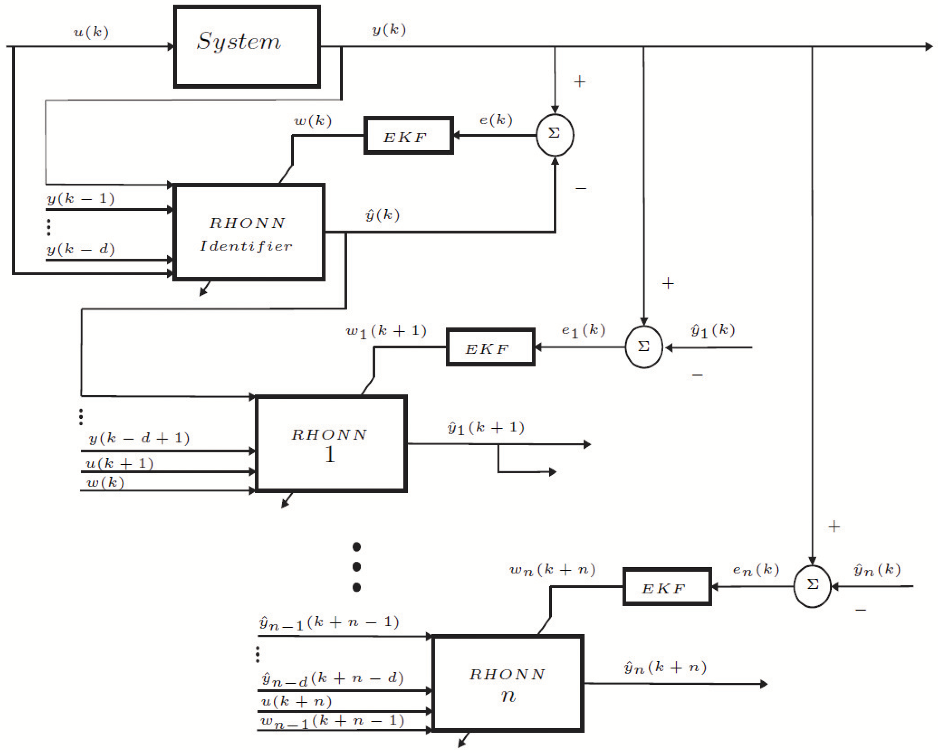
The real-time training of the recurrent neural network based on the EKF allows adjusting the weights with the value observed in time k, which is the system information in $y\left(k\right)$ and the neural network output $\widehat{y}\left(k\right)$. Consequently, the RHONN represents a model of the wind speed trend at time k, and the weight adjustment process of the model is carried out continuously in each new observed sample. In this way, we consider n RHONN identical to the identified model and to recursively produce a prediction up to the n prediction horizon.

Then, to prevent the forecasting from guessing near the mean distribution, each neural network $\{r=1,\dots ,n\}$ adjusts its weights individually through the differences between the available observed values and those predicted. The prediction error of the RHONN r used to reinforce the adjustment of the weights is calculated as follows:

$$e_r\left(k\right)=y_r\left(k\right)-{\widehat{y}}_r\left(k\right),r=1,\dots ,n,$$

(14)

where $e_r$ represents the error of each NN, ${\widehat{y}}_r$ represents the output forecast value by the r NN. All the neural networks reinforce their weights using the EKF algorithm with their respective prediction error $e_r\left(k\right)$ once the observed value can be compared with the prediction produced. In this way, it is not possible to adjust the weights in the first prediction steps since the observed value is not available to calculate the error. Figure 1 shows the graphical representation of the implemented structure of the RHONN to forecast multiple steps forward and the on-line reinforcement of the neural network weights.

3. Results

In this section, the proposed methodology is applied for the forecasting of nine different time series. For this work, we use freely available datasets, and their application shows the performance of the proposed methodology in obtaining an accurate performance for short-term time series forecasting. First, the proposed method is applied to the problem of forecasting the wind speed and wind-generated power. Then, the proposed approach is used for forecasting energy price with data from seven different countries.

3.1. Proposed Methodology

In this section, the proposed methodology for time series forecasting in wind energy systems is explained. The methodology depicted in Figure 1 was modified to be applied to time series forecasting, and this modification is depicted in Figure 2, which shows the graphical representation of the proposed methodology for time series forecasting applied to wind energy systems. To start with the forecasting process, it is necessary to have at least d past values from time series data. This value is defined as the system dimension, and in this work, it is defined using the Cao methodology [31]. The input values for the first RHONN are defined as ($y(k-1),y(k-2),\dots ,y(k-d)$. With these values, it is possible to forecast the value $\widehat{y}\left(k\right)$, and then, this value feeds the next RHONN to forecast the value $\widehat{y}(k+1)$. By applying this methodology successively until to RHONN number n, it is possible to obtain the forecasting of n future values of the used time series. The value n depends on the chaotic behavior of the used data and of their application.

The training for each RHONN is developed on-line; therefore, there is no stopping criterion nor necessary retraining for the proposed RHONNs. It is important to note that for the proposals of this paper, only the output of the RHONN n is depicted as the n-step-ahead forecasting result for each one of the used time series, as described in [29]. RHONN are not defined with a layer structure; they are defined with a dynamic model. Furthermore, it is relevant to note that, in this case, as the training algorithm works on-line, all data are used for training as well as for validation, and there is no pre-training stage. Furthermore, due to the stochastic nature of the EKF training algorithm, it is not necessary to do any data pre-processing or normalization as data are used as-obtained from repositories, which is another highlight of the proposed methodology. The proposed methodology of n RHONN trained with an EKF- based algorithm was coded in Matlab^® 2016a and implemented in an Intel^® Core™ Processor, i7-6820HQ [email protected] GHz, 2701 Mhz, 4 Core(s), 8 Logical Processor(s) with Microsoft Windows 10 Pro^®.

3.2. Data Explanation

In order to test the applicability of the proposed methodology, nine different time series related to wind energy systems were selected, and all of them are considered nonlinear, chaotic, time-variant and non-stationary [5,6]. The data were recovered from open-access repositories that can be found in [32,33] for wind speed and energy prices, respectively. Each dataset is composed of a large amount of data, but in this work, we are only considering a short period in order to test the applicability of the proposed methodology. It is relevant to comment that the selected period of the used time series can be easily modified, and the data were selected only for applicability purposes due to the open-access availability. There were no missing data or any abnormal values detected, and the processing of missing or abnormal data is out of the scope of this work. For a detailed explanation of the methodology used to obtain and process these datasets, please refer to [32,33].

3.3. Wind Speed and Power Forecasting

The proposed methodology was applied for forecasting time series of wind speed. The wind speed data are available in [32], and the selected period begins on 1 September 2020 at 01:00:00 with a sampling time of 1 h, with 500 values. This interval was only selected to test the applicability and can be easily modified. Figure 3 depicts in red the actual values for the time series data for wind speed used to test the proposed methodology. For forecasting, a RHONN (5) was used, which was trained with an EKF based-algorithm (9). The RHONN was connected, as shown in Figure 2, with 15 RHONNs, with one for each step to be forecasted. Each of them contains 20 neurons with a hyperbolic tangent activation function. The EKF parameters were selected as: $P\left(0\right)=1.0$, $R\left(0\right)=1\times {10}^{-2}$ and $P\left(0\right)=1\times {10}^{-6}$. The training was performed on-line with seven past measurements to perform the 15-step-ahead forecasting. The obtained results for a 15-step-ahead forecasting are presented in Figure 3, which includes real wind speed values at the top in red, the 15 step-ahead forecast values at the top in blue and the forecasting error at the bottom.

Now, the forecast of wind speed is used to calculate produced power using a wind turbine model, as shown in Figure 4. To obtain this estimation, the “Simple Turbine Block” of Simscape from Simulink of Matlab was used. The Simple Turbine Block converts wind speed to turbine output power by a simple output power versus wind speed characteristic. When the wind speed is below the cut-in speed or above the cut-out speed, the machine generates zero real power [34]. In this case, the selected parameters are defined in

Table 1. Wind turbine parameters.

Parameter	Value
Rated output power	150 kW
Cut-in speed	3 m/s
Rated output speed	12 m/s
Cut-out speed	23 m/s

. Calculated produced power is displayed in Figure 5, which includes emulated wind power values at the top in red, the 15 step-ahead forecast values at the top in blue and the forecasting error at the bottom. From Figure 3 and Figure 5, the excellent capability of the proposed RHONN structure to forecast the performance of time series for speed with real-world data for a wind energy system can be observed. It is important to note that this forecasting method gives information about very short and short-term forecasts, and these data can be used to improve control performance as well as for planning, production, management and marketing.

3.4. Energy Price Forecasting

Another very useful time series in wind energy systems is the energy price, which is crucial for management and marketing. This forecast allows the producers to make adequate decisions regarding the purchase and sale of energy. The used time series data are available in [33]. The selected period begins on 1 September 2020 at 01:00:00 with a sampling time of 1 h, with 700 values. This interval was only selected to test the applicability and can be easily modified. The data belong to information of seven different countries: Denmark, Germany, Ireland, Italy, Norway, Sweden and the United Kingdom. For forecasting, a RHONN (5) was used and trained with an EKF-based algorithm (9). The RHONN was connected, as in Figure 2, with 15 RHONNs, with one for each step to be forecasted. Each of them contains 20 neurons with a hyperbolic tangent activation function. The EKF parameters were selected as: $P\left(0\right)=1.0$, $R\left(0\right)=1\times {10}^{-2}$ and $P\left(0\right)=1\times {10}^{-6}$. The training was performed on-line with seven past measurements to perform the 15-step-ahead forecasting. The obtained results for a 15-step-ahead forecasting are presented in Figure 6, Figure 7, Figure 8, Figure 9, Figure 10, Figure 11 and Figure 12, and they include real energy price values at the top in red, the 15 step-ahead forecast values at the top in blue and the forecasting error at the bottom for each one of the selected time series. For each one of the selected time series, it can be seen that the forecasting error is near to zero with small variation. These results are analyzed in Section 4. Furthermore, Figure 6, Figure 7, Figure 8, Figure 9, Figure 10, Figure 11 and Figure 12 show the excellent capability of the proposed RHONN structure to forecast the performance of the time series for energy price with real-world data for a wind energy system.

4. Analysis and Discussion

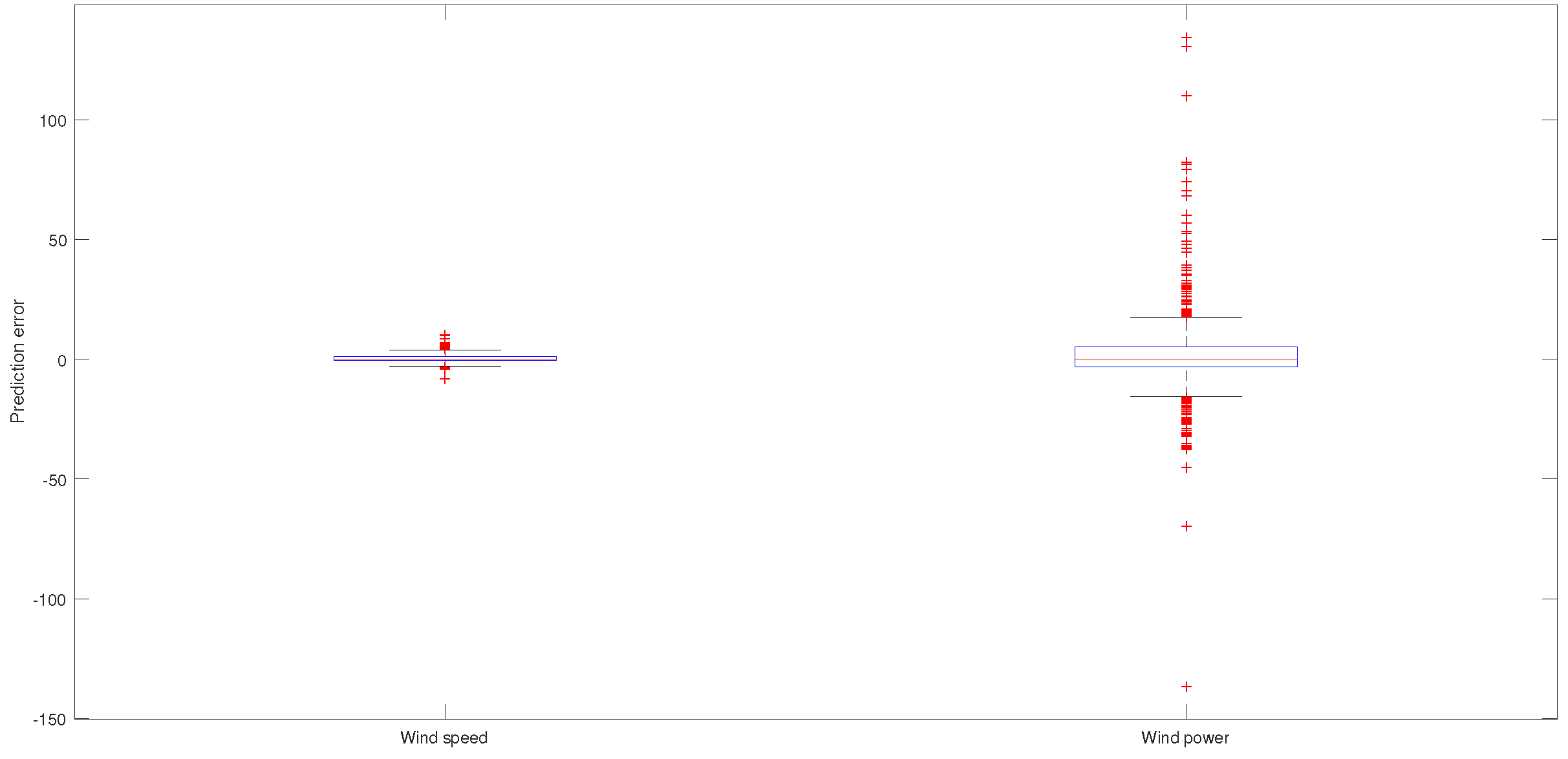
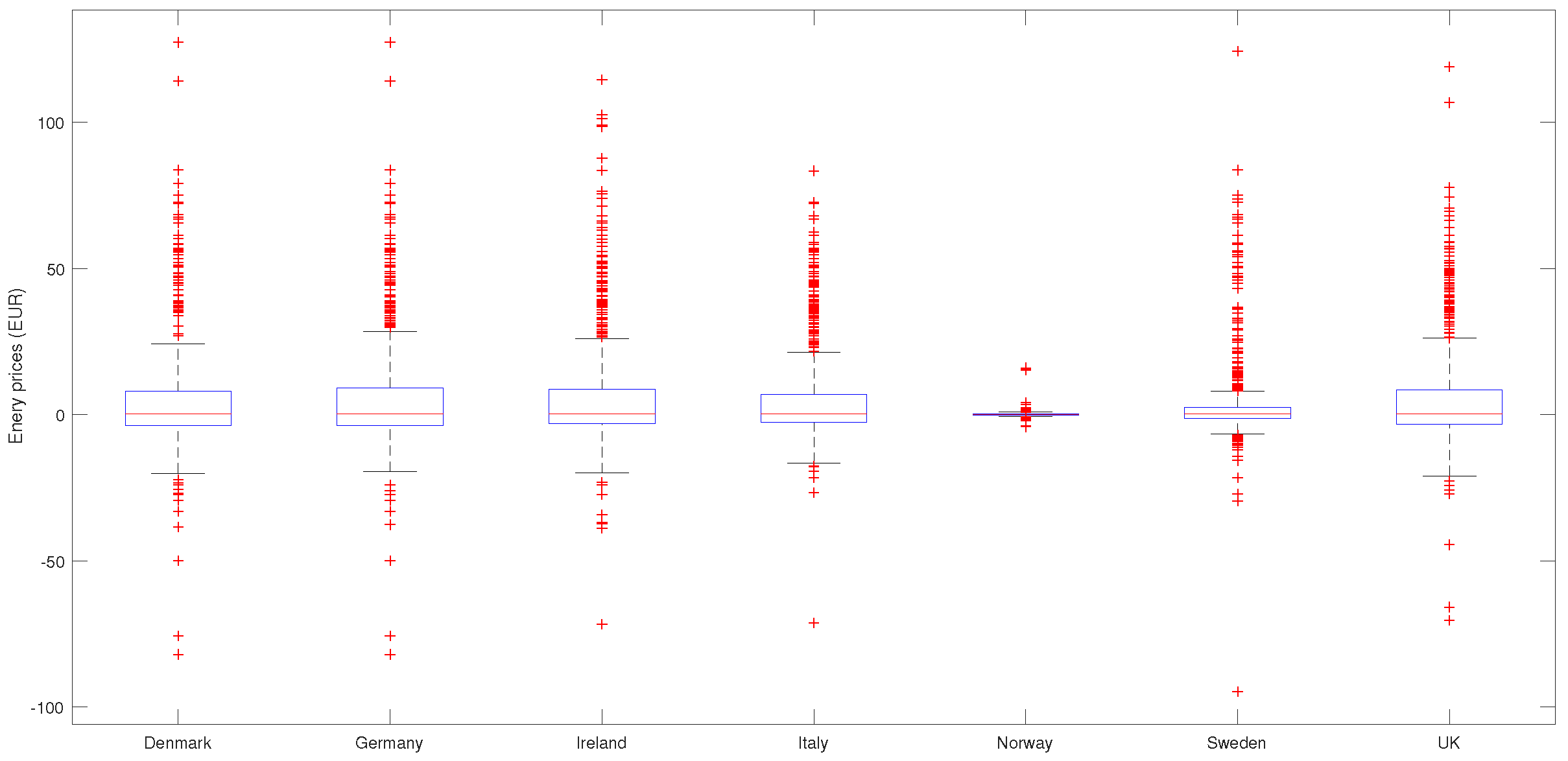
In this section, the obtained forecasting results are analyzed. First, Figure 13 and Figure 14 present a box plot for each one of the selected time series. This kind of plot is used to show the distribution of a dataset [35]. Figure 13 shows wind speed and generated power error forecasting variations, and it is easy to see that the obtained results present forecasting errors with a mean value around zero with acceptable variation. 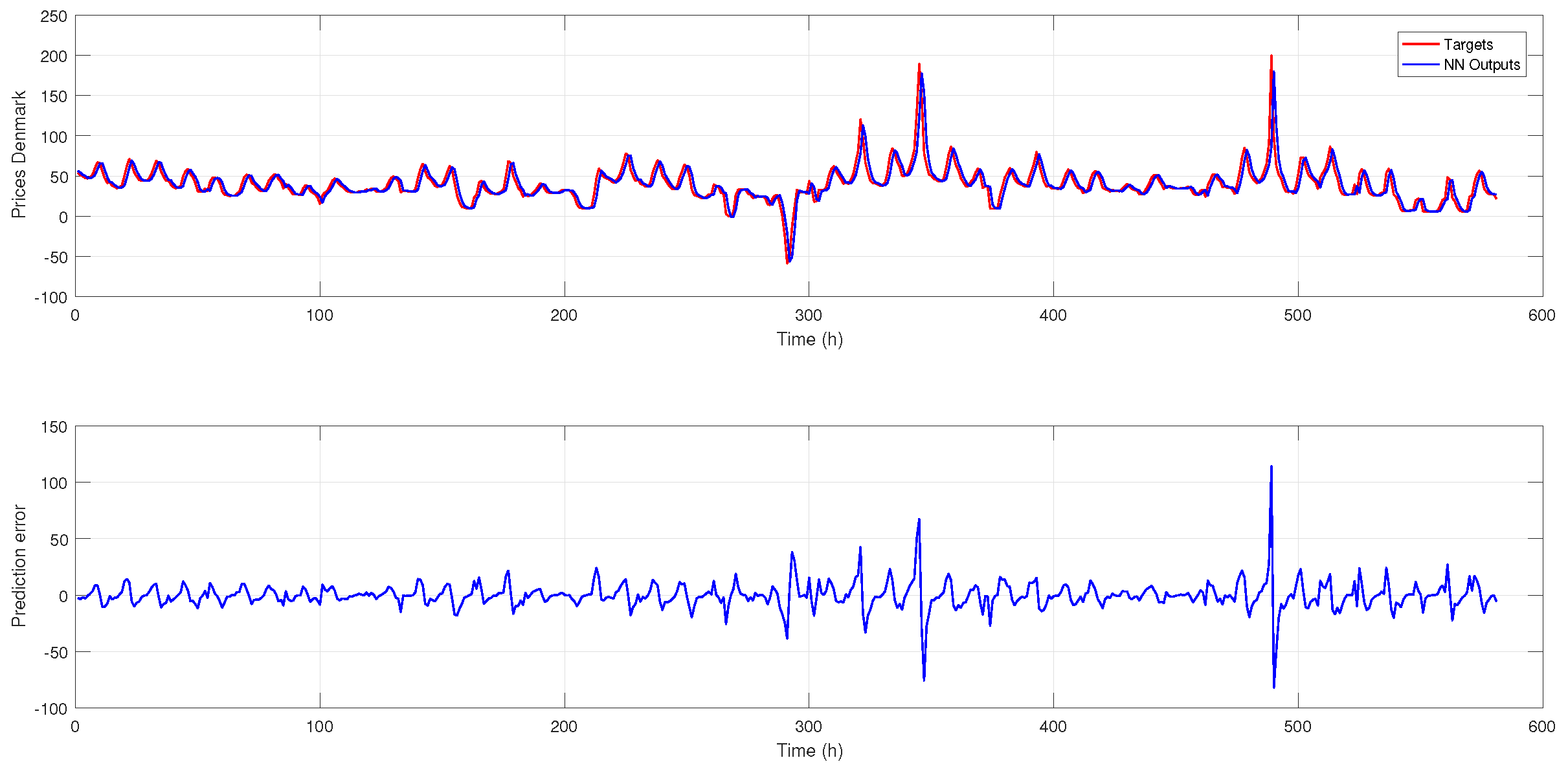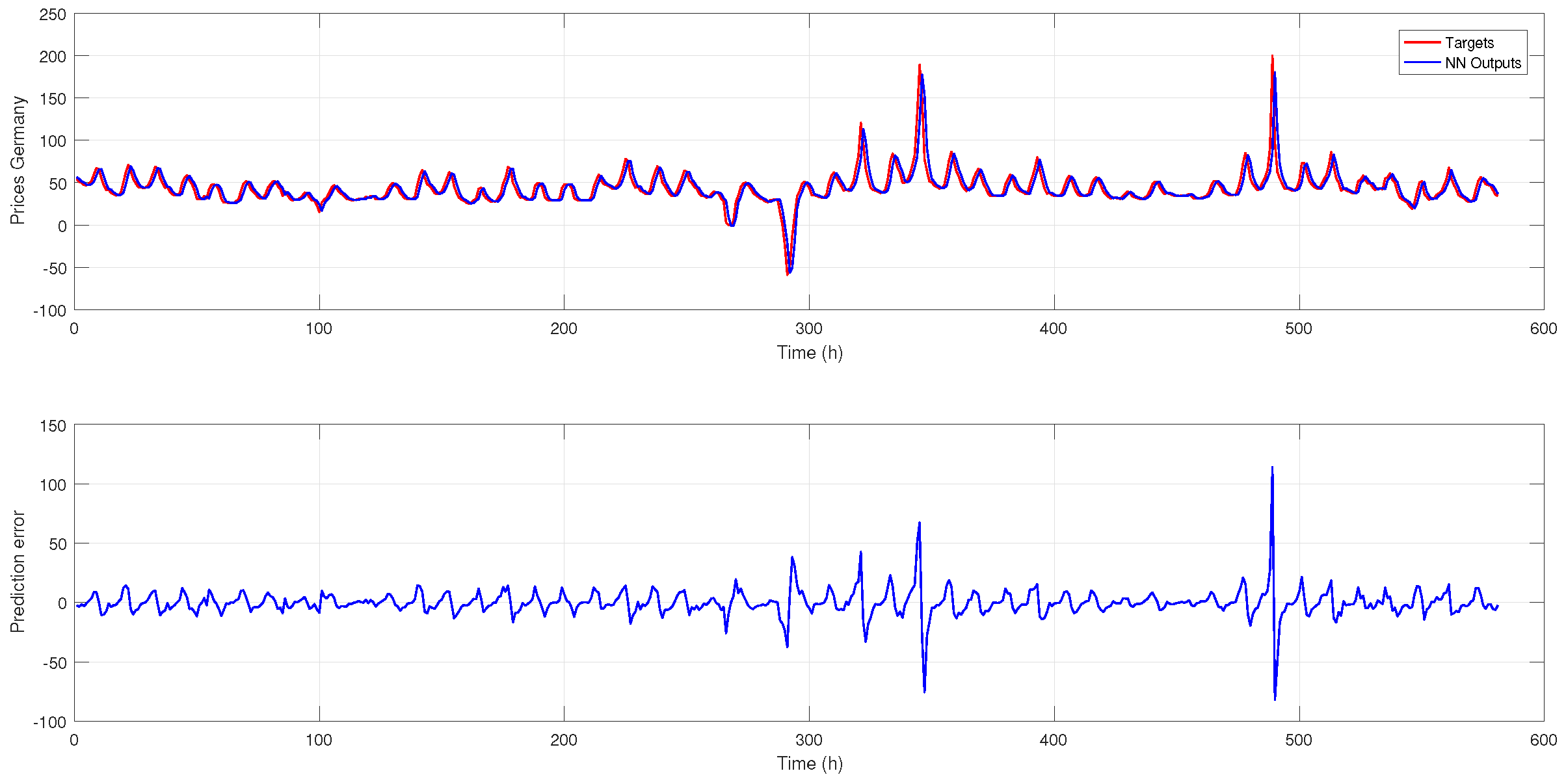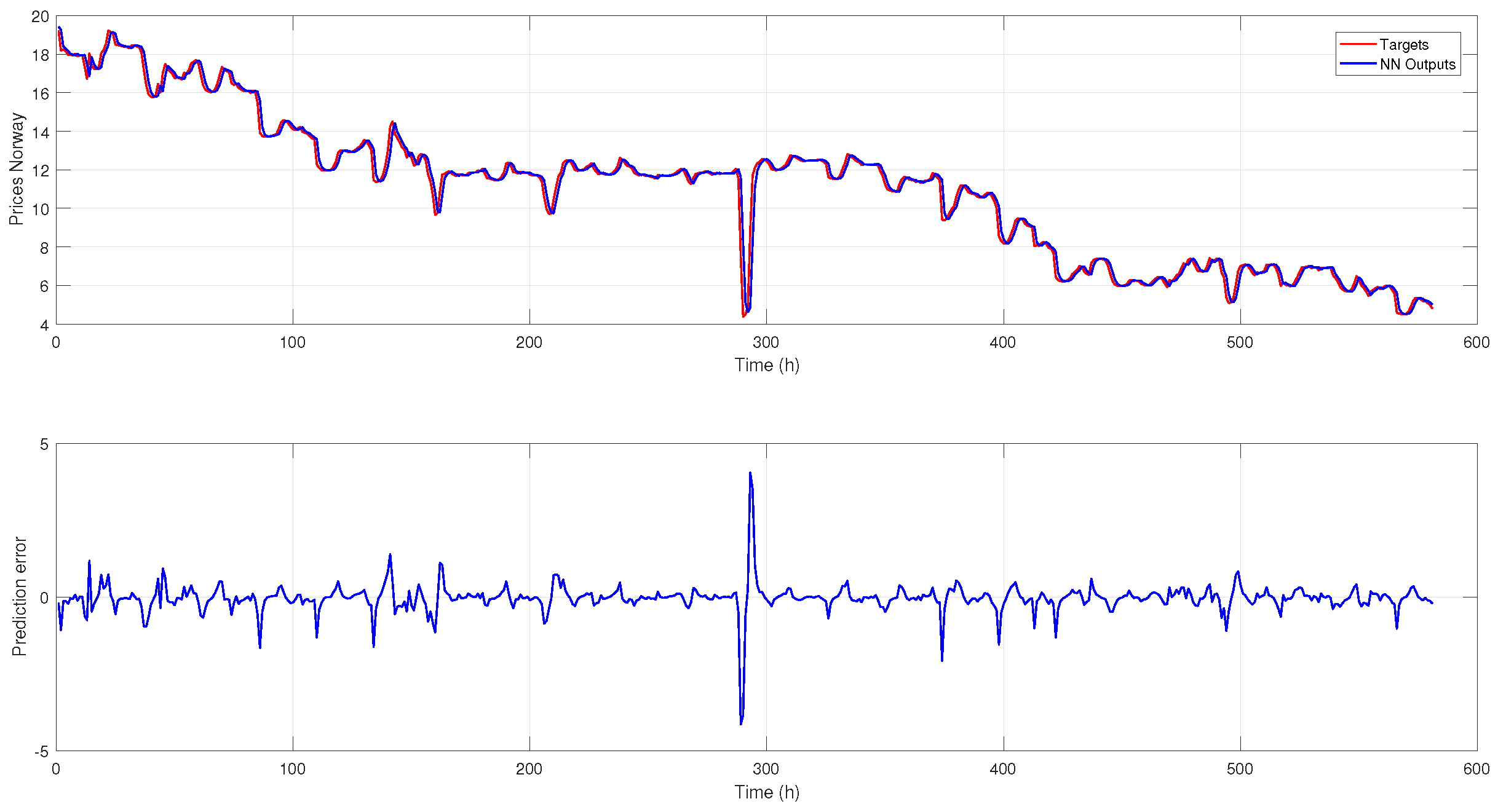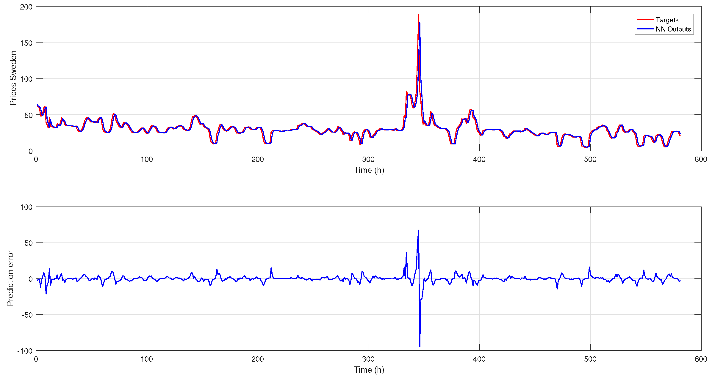Similar results can be seen in Figure 14 for energy price error forecasting, and in this last figure, it can be seen that the lower variation was obtained for Norway, and the largest variation was obtained for Denmark. This could be due to the presence of outliers. Second, in

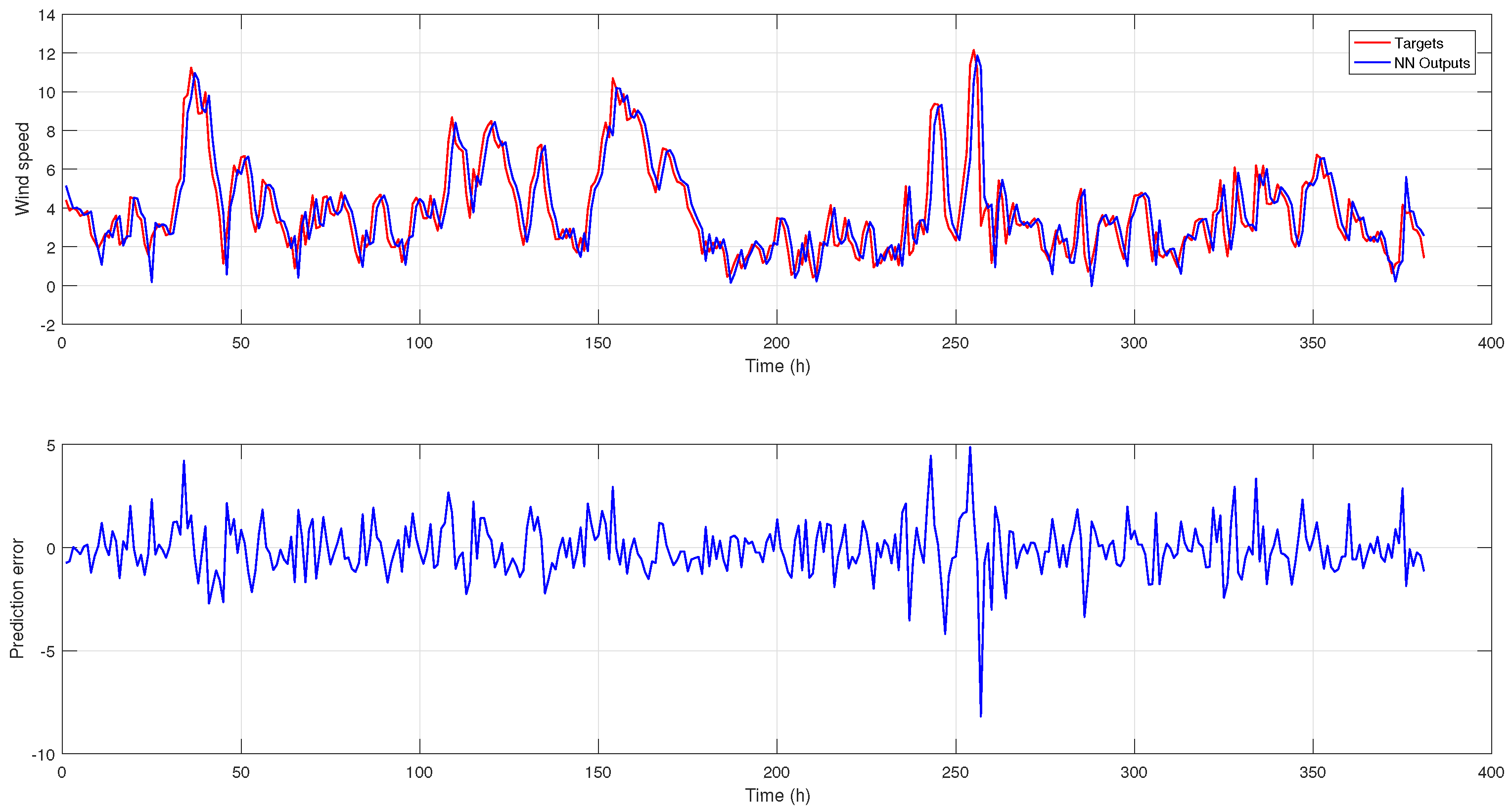
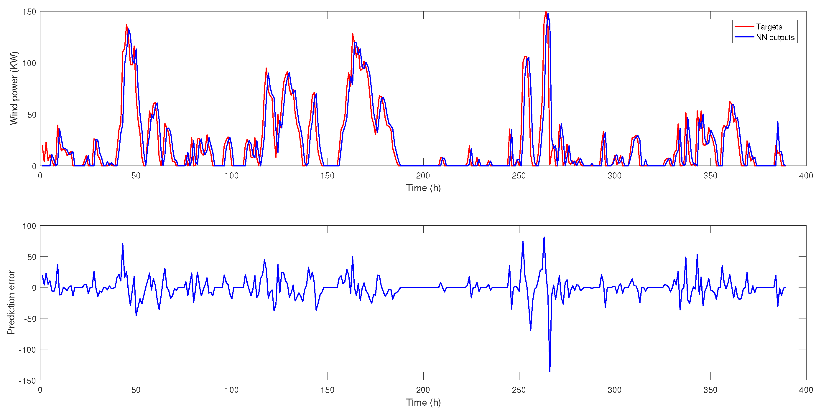
Table 2. Statistical information for time series forecasting errors.

Time Series	MSE	RMSE	MEAN	MAPE
Wind speed	1.5880	1.2601	−0.0545	3.7490
Wind power generation	216.0227	14.6977	−0.5101	1.9425
Energy price for Denmark	140.9990	11.8743	−0.1090	2.1913
Energy price for Germany	125.6029	11.2073	−0.0821	3.0339
Energy price for Ireland	5.5595	9.7755	−0.0819	3.3643
Energy price for Italy	51.8081	7.1978	−0.0145	3.7549
Energy price for Norway	0.2137	0.4623	−0.0349	1.2815
Energy price for Sweden	47.0634	6.8603	−0.0977	2.1032
Energy price for the UK	97.4408	9.8712	−0.0475	3.2192

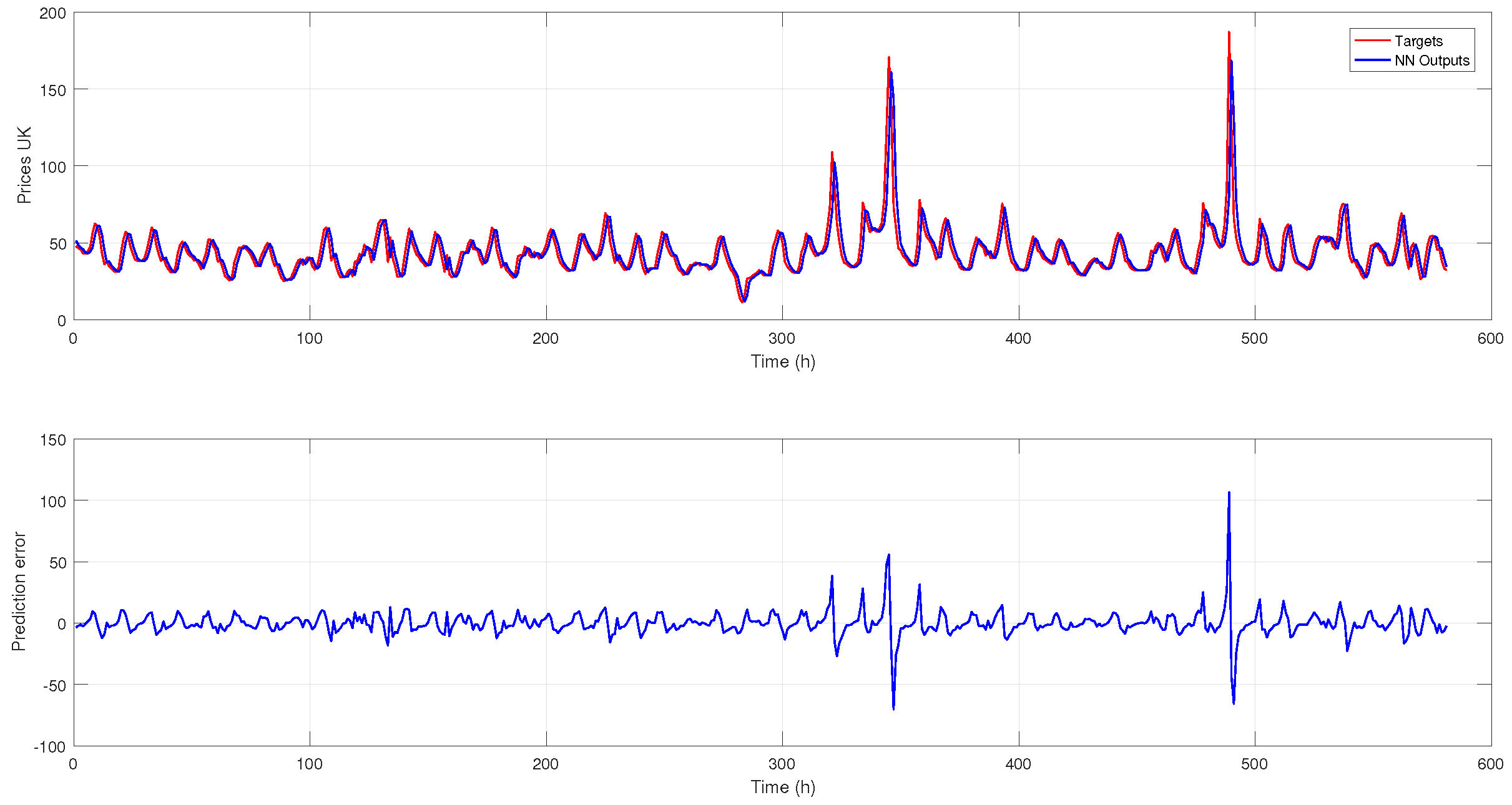
, statistical information for the forecasting error is included, which is depicted in Figure 3 and Figure 5, Figure 6, Figure 7, Figure 8, Figure 9, Figure 10, Figure 11 and Figure 12; moreover, Table 2 includes the mean square error (MSE), root mean square error (RMSE), mean and mean absolute percentage error (MAPE). From this information, it is easy to see that energy price forecasting for Norway presents the best performance. The calculations are based on the relative error $e\left(k\right)$ as defined in (12), and the statistical information was calculated in order to quantitatively determine the best model, according to [2,35], as follows:

$$\begin{array}{ccc}\hfill MSE& =& \frac{1}{n}\sum _{k=1}^n{\left(e\left(k\right)\right)}^2\hfill \end{array}$$

(15)

$$\begin{array}{ccc}\hfill RMSE& =& \sqrt{MSE}\hfill \end{array}$$

(16)

$$\begin{array}{ccc}\hfill MEAN& =& \frac{1}{n}\sum _{k=1}^n\left(e\left(k\right)\right)\hfill \end{array}$$

(17)

$$\begin{array}{ccc}\hfill MAPE& =& \frac{1}{n}\sum _{k=1}^n\frac{e\left(k\right)}{y\left(k\right)}\hfill \end{array}$$

(18)

Table 3. MAPE for time series forecasting for n-step-ahead forecasting.

Time Series	$\mathit{n}=1$	$\mathit{n}=5$	$\mathit{n}=9$	$\mathit{n}=13$	$\mathit{n}=14$	$\mathit{n}=15$
Wind speed	0.2311	0.5362	1.1369	1.4593	1.4660	1.9425
Wind power generation	0.5197	0.9413	2.0515	3.3400	3.4838	3.7490
Energy price for Denmark	0.1182	0.8337	1.2443	1.6593	1.8206	2.1913
Energy price for Germany	0.0361	0.7978	1.6035	2.3639	2.4098	3.0339
Energy price for Ireland	0.0156	0.5126	1.8111	3.0727	3.2361	3.3643
Energy price for Italy	0.3171	0.9758	2.1767	3.2619	3.2641	3.7549
Energy price for Norway	0.0636	0.2357	0.5149	0.7972	1.0932	1.2815
Energy price for Sweden	0.2029	0.7103	1.0290	1.9813	1.9871	2.1032
Energy price for the UK	0.0496	0.7558	1.7609	2.3555	2.3973	3.2192

presents MAPE. This performance criterion was selected due to the managerial appeal and is a measure commonly used in forecasting [35]. In this table, the percentile errors for different forecasting horizons can be seen. It is easy to see that for $n\le 15$, the percentile error remains below 5% due to the fact that $n=15$ is the forecasting horizon selected in this paper; for $n>15$, the obtained performance has percentile error over $5\%$, and for the purpose of this paper, it is considered a poor performance.

In order to make a comparison of the proposed methodology with respect to existing ones, it is important to note from Table 3 that, for $n=1$, the percentile error is below $0.6\%$, and for the same scenario in [21], the reported $MAPE$ is $3\%$. In addition, the proposed methodology has a better computational complexity, and in this approach, the forecasting horizon can be easily extended, as exemplified by the different examples presented in this paper. These results are important as they show the effectiveness of the proposed scheme with a high forecasting accuracy. Even for a forecasting horizon beyond this one, the existence of an accurate and reliable forecasting methodology, such as the proposed one, allows for the application to energy systems management, planification, energy dispatch improvements, scheduling and design of control systems, and can provide benefits for energy producers, users and operators.

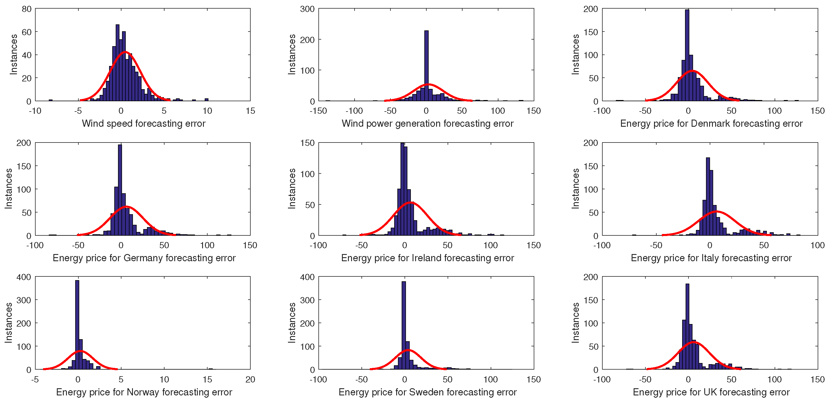
Figure 15 shows error histograms for the nine used time series. From this figure, it can be seen that the obtained forecasting errors do not have a Gaussian distribution. However, error values are around zero with a low standard deviation, which confirms the information obtained in Figure 13 and Figure 14 as well as the information contained in Table 2. All of this information confirms the forecasting capabilities of the proposed scheme independent of the nature of the data; thus, it is possible to infer that the proposed methodology can be applied to forecast a different type of time series.

5. Conclusions

This paper proposes the use of a RHONN trained with an EKF learning algorithm for energy time series forecasting, which includes wind speed, wind power generated and energy prices. All results obtained shown in Table 2 present a good performance for each case. The proposed methodology is simple in structure, which allows an on-line implementation to forecast multiple steps forward, despite the highly nonlinear nature of the system, in which it is extremely beneficial to know future values. It is important to note that, unlike most modern forecasting techniques, the proposed methodology stands out for its simplicity and for having low computational complexity, producing very good results, as shown by the included results. The obtained results show that forecasting for time series on wind energy systems is not a simple task; however, the proposed neural methodology captures complex dynamics, including nonlinearities, chaos, noise and uncertainties. The forecasting results help to operate the energy systems, satisfy the energy demand, optimize the power supplied to the utility grid, maximize the energy supplied by renewable sources and minimize the energy supplied by non-renewable sources. It is important to highlight that the forecast results obtained in this work are relevant because the proposed methodology does not require prior data treatment, nor does it require information external to the time series data. Because the training is on-line, only seven past measurements are required to start the forecasting process, being able to achieve a forecast of up to 15 steps forward. This completely differs from existing methodologies, which require off-line training to achieve a forecasting horizon beyond this one, in addition to incorporating external information to the time series. Finally, they are models with high computational complexity that require very long processing times and the use of highly specialized computer equipment, and these are requirements that are not necessary for the proposed methodology. All these improvements show the importance of the proposed methodology for time series forecasting. The used data do not contain missing or abnormal data; therefore, time series with this kind of problem can be considered in future work. At this time, the authors are working on using the forecasted time series to simulate a closed-loop wind energy system, including an electric generator dynamic, gearbox dynamic, converter, main grid parameters and other elements that complete the whole wind energy system.