A New Smoothness Indicator of Adaptive Order Weighted Essentially Non-Oscillatory Scheme for Hyperbolic Conservation Laws

Abstract

Adaptive order weighted essentially non-oscillatory scheme (WENO-AO(5,3)) has increased the computational cost and complexity of the classic fifth-order WENO scheme by introducing a complicated smoothness indicator for fifth-order linear reconstruction. This smoothness indicator is based on convex combination of three third-order linear reconstructions and fifth-order linear reconstruction. Therefore, this paper proposes a new simple smoothness indicator for fifth-order linear reconstruction. The devised smoothness indicator linearly combines the existing smoothness indicators of third-order linear reconstructions, which reduces the complexity of that of WENO-AO(5,3) scheme. Then WENO-AO(5,3) scheme is modified to WENO-O scheme with new and simple formulation. Numerical experiments in 1-D and 2-D were run to demonstrate the accuracy and efficacy of the proposed scheme in which WENO-O scheme was compared with original WENO-AO(5,3) scheme along with WENO-AO-N, WENO-Z, and WENO-JS schemes. The results reveal that the proposed WENO-O scheme is not only comparable to the original scheme in terms of accuracy and efficacy but also decreases its computational cost and complexity.

1. Introduction

It is well known that capturing shock waves in compressible flows remains a challenging issue to numerical schemes in computational fluid dynamics due to the coexistence of smooth and discontinuous structure of different scales. Thus, though the initial conditions of hyperbolic conservation laws are smooth, discontinuities might be developed in the solution. As a result, Taylor expansion-based numerical schemes fail to estimate hyperbolic conservation law solutions. Therefore, alternative schemes are proposed to realize the approximate solution without introducing spurious oscillations based on adaptively selecting the smoothest stencil among several candidates that are Essentially Non-Oscillatory (ENO) schemes. In these schemes, based on finite volume framework, Harten et al. [1] devised the concept of smoothness indicator to measure the smoothness of each interpolation polynomial and then select the smoothest stencil over different candidate stencils. Thereafter, based on finite difference discretization, Shu & Osher [2] introduced a more efficient variant of ENO schemes by directly using upwinding to the fluxes on basis of dimension-by-dimension.

In addition, a new class of ENO scheme was devised first by Liu et al. [3] and then enhanced by Jiang and Shu [4] by using more efficient smoothness indicator to reach the optimal order accuracy in smooth region. These schemes employing all candidate sub-stencils of ENO scheme by convex combination in a non-linear manner instead of choosing the smoothest one; then for each sub-stencil, a weight is assigned according to its local smoothness indicator. Therefore, these schemes are known as Weighted Essentially Non-Oscillatory (WENO) schemes. In these schemes, the basic idea of using non-linear weights is automatically ignoring the sub-stencil that contains discontinuities by assigning small weight to its polynomial while using optimal weights to each sub-stencil’s polynomial in convex combination to produce, for smooth regions, an upwind scheme of maximum possible order of accuracy.

Later in 2005, Henrick et al. [5] have done analysis to the fifth-order WENO scheme and found that the scheme does not obtain the desired order of convergence and then loses its optimal order accuracy at critical points where the solution’s first derivative vanishes. Thus, they developed a strategy to recover the optimal order accuracy of WENO schemes at critical point which maps the original weights to new weights by using mapping function, the modified scheme was known as mapped WENO scheme (WENO-M). Moreover, they derived the sufficient condition which is used as guidance to test and design the weights of improved WENO schemes since then. Nevertheless, WENO-M scheme enlarges the effect from non-smooth stencils then, near discontinuities, a potential loss of accuracy might take place. Moreover, it increases the computational cost. Furthermore, a new strategy to recover the optimal order accuracy at critical points is proposed by Borges et al. [6] whereas higher-order global smoothness indicator is obtained from existing original smoothness indicators. Thus, a new non-linear weight is devised which reduces the computational cost and improves the numerical solution of WENO-M scheme with less dissipative rate. They abbreviate the improved scheme as WENO-Z scheme.

Recently, WENO schemes are becoming popular numerical schemes for solving complex flows such as shock-turbulence interaction due to their capability for resolving discontinuities without numerical oscillations and high-order accuracy [7]. Many efforts have been made to improve classic WENO schemes such as WENO-ZQ [8], WENO-AO [9], WENO-$\theta$ [10], RBF-WENO [11], WENO-$\eta$ [12], CWENO-2D [13], ESWENO [14] schemes, and others (see for instance [15,16,17,18,19,20,21,22,23] and the references therein). Among them, this paper will focus on improving the WENO-AO scheme [9]. The idea of adaptive order is first proposed by [8] whereas a new convex combination of two linear polynomials and fourth-degree polynomial is introduced. This demonstrates superior performance over classic WENO (WENO-JS) scheme in terms of order accuracy. Thereafter, a convex combination of fourth-degree polynomial and three quadratic polynomials is used by Balsara et al. [9] to propose new adaptive fifth-order WENO scheme of known as WENO-AO(5,3). Moreover, they used Legendre polynomials to calculate the smoothness indicators.

Although this scheme enhances the accuracy of classic WENO scheme, it increases the computational cost since it involves computing new smoothness indicator for the fourth-degree polynomial. It is known that in the whole computation, the heaver part is calculating the smoothness indicators. Therefore, in WENO-AO(5,3) scheme, calculation of smoothness indicator of fifth-order linear reconstructions increases the computational cost. Moreover, it is difficult to obtain the explicit form of extra smoothness indicator for non-uniform mesh. For that reason, a non-linear convex combination of existing smoothness indicators for the three third-order linear reconstructions was proposed in [24] to compute the extra fifth-order linear smoothness indicator, and denoted the new scheme as WENO-AO-N. This method not only reduces the computational cost, but also demonstrates high accuracy without non-physical oscillations. This motivates the current paper to further reduce the computational cost of WENO-AO-N and then WENO-AO(5,3). Moreover, further increase of the accuracy without non-physical oscillations, by introducing new and simple smoothness indicator for the largest stencil.

This paper proposes new and simple smoothness indicator of the fifth-order linear reconstructions for WENO-AO(5,3) scheme and then modifies it with simple formulation. The devised simple smoothness indicator is following the idea of linearly combining the existing smoothness indicators of third-order linear reconstructions. Therefore, it is simple in the explicit form since it uses existing sub-stencils smoothness indicators unlike WENO-AO(5,3) scheme. Moreover, it is without non-linear convex combination and complex coefficients as introduced in WENO-AO-N scheme. We abbreviate the new scheme as WENO-O scheme.

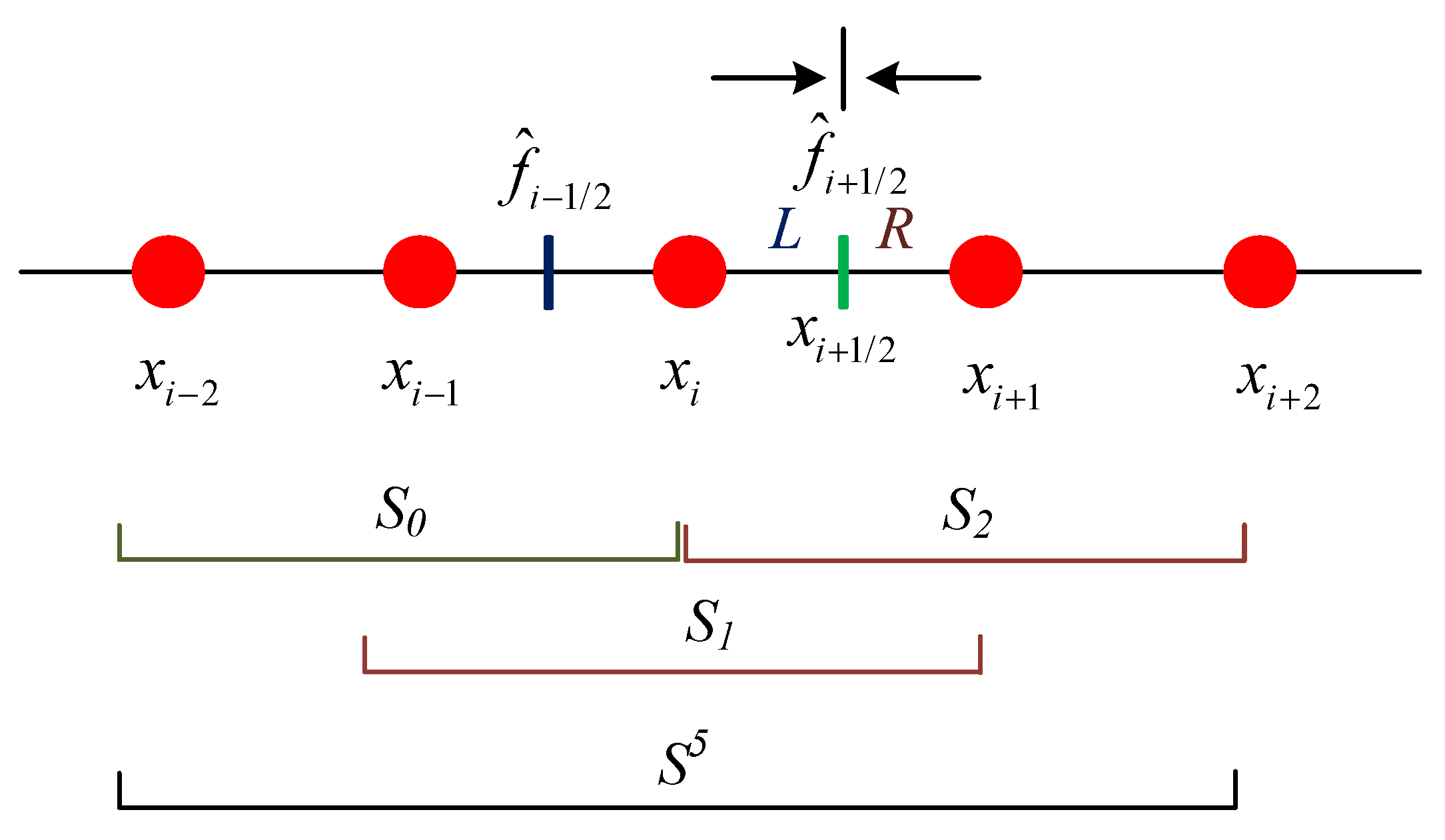
2. Finite Difference WENO Schemes

For the sake of simplicity, we adopted 1-D scalar hyperbolic conservation law

$$\left\{\begin{array}{c}{u}_t+f_x\left(u\right)=0,x\in \left[x_l,x_r\right],\\ u(x,0)=u_0\left(x\right),\end{array}\right.$$

(1)

where u is the conservative variables and $f\left(u\right)$ is the flux vector. Equation (1) can be a system or a single equation. The semi-discrete finite difference scheme of (1) is

$$\frac{d{u}_i\left(t\right)}{dt}=R{\left(u\right)}_i,$$

(2)

and $u_i\left(t\right)$ denotes the numerical approximation to the point value of $u(x_i,t)$, $R{\left(u\right)}_i$ is given by:

$$R{\left(u\right)}_i=-\frac{1}{h}({\widehat{f}}_{i+1/2}-{\widehat{f}}_{i-1/2}),$$

(3)

where ${\widehat{f}}_{i\pm 1/2}$ represent numerical fluxes at the cell boundaries that are calculated using a numerical scheme (see Figure 1). Here we consider uniform mesh to divide the spatial domain, i.e., $h=x_{i+1}-x_i,x_{i+1/2}=x_i+h/2$ and the cells are denoted by $I_i=\left[x_{i-1/2},x_{i+1/2}\right]$. The property of conservation is obtained by implicitly defining the function $v\left(x\right)$ through:

$$f\left(u\left(x\right)\right)=\frac{1}{h}\underset{x-h/2}{\overset{x+h/2}{\int }}v\left(x\right)dx,$$

(4)

where $v\left(x\right)$ approximates the numerical flux ${\widehat{f}}_{i\pm 1/2}$ with a high order of accuracy, i.e.,

$${\widehat{f}}_{i+1/2}=v\left(x_{i+1/2}\right)+\mathrm{O}\left(\mathsf{\Delta }x\right).$$

(5)

To ensure the numerical stability, the flux $f\left(u\right)$ is split into two parts $f^{+}\left(u\right)$ and $f^{-}\left(u\right)$ with $\frac{d{f}^{+}\left(u\right)}{du}\ge 0$ and $\frac{d{f}^{-}\left(u\right)}{du}\le 0$, using the global Lax-Friedrichs flux splitting method as

$${\widehat{f}}_{i+1/2}^{\pm }=\frac{1}{2}(f\left(u\right)\pm \alpha u),$$

(6)

where $\alpha$ is taken as ${max}_u\left|f^{{}^{\prime }}\left(u\right)\right|$ and ${\widehat{f}}_{i+1/2}={\widehat{f}}_{i+1/2}^{-}+{\widehat{f}}_{i+1/2}^{+}$. Since ${\widehat{f}}_{i+1/2}^{-}$ is symmetric to the positive part with respect to $x_{i+1/2}$, from here onwards, we will only describe how ${\widehat{f}}_{i+1/2}^{+}$ is constructed and the “+” sign in the superscript will be dropped for convenience.

2.1. Fifth-Order WENO-JS Scheme

Basically, WENO schemes [4] are designed to approximate the spatial derivative for solving the hyperbolic conservation laws in essentially non-oscillatory manner. In the fifth-order WENO scheme, the five-points stencil $S^5= \left\{x_{i-2},x_{i-1},x_i,x_{i+1},x_{i+2}\right\}$ is subdivided into three candidate sub-stencils $S_0= \left\{x_{i-2},x_{i-1},x_i\right\}$, $S_1= \left\{x_{i-1},x_i,x_{i+1}\right\},$ and $S_2= \left\{x_i,x_{i+1},x_{i+2}\right\}$ then a convex combination (7) of sub-stencils flux functions is used to reconstruct the flux function ${\widehat{f}}_{i+1/2}$ at the cell $I_i$ interface $x_{i+1/2}$. The main difference between WENO and ENO schemes is that WENO schemes use the convex combination of sub-stencils flux functions instead of using smoothest sub-stencil, which is written as

$${\widehat{f}}_{i+1/2}=\sum _{k=0}^2{\omega }_k{\widehat{f}}^k\left(x_{i+1/2}\right).$$

(7)

The WENO non-linear weights ${\omega }_k$ (8) are designed to approach very small value when the corresponding sub-stencil contains a discontinuity and approach the optimal value for smooth solution.

$${\omega }_k=\frac{{\alpha }_k}{{\sum }_{l=0}^2{\alpha }_l},{\alpha }_k=\frac{d_k}{{({\beta }_k+\epsilon )}^p},$$

(8)

where ${\alpha }_k$ ($k=0,1,2$) are referred to as the un-normalized weights, $\epsilon$ is small number used to prevent division by zero, $p=2$. To measure the smoothness of a solution over a particular sub-stencil, the smoothness indicators ${\beta }_k$ are employed which are given by:

$${\beta }_k=\sum _{l=1}^{r-1}\mathsf{\Delta }{x}^{2l-1}\underset{x_{i-1/2}}{\overset{x_{i+1/2}}{\int }}{\left(\frac{d^l}{d{x}^l}{\widehat{f}}^k\right)}^{2}dx.$$

(9)

In addition, $d_k$ represent the ideal/optimal weights as they create the upstream central fifth-order scheme for the five-point stencil in smooth regions as

$${\widehat{f}}_{i+1/2}^5=\sum _{k=0}^2{d}_k{\widehat{f}}^k\left(x_{i+1/2}\right).$$

(10)

The flux function ${\widehat{f}}_{i+1/2}$ of the cell interface is reconstructed using sub-stencils’ polynomials ${\widehat{f}}^k\left(x_{i+1/2}\right)$ as in (11). The values of ideal weights are given by $d_0=0.1,$ $d_1=0.6$, $d_2=0.3$ and

$$\begin{array}{c}{\widehat{f}}_{i+1/2}^0=\frac{1}{6}\left(2g_{i-2}-7g_{i-1}+11g_i\right),\hfill \\ {\widehat{f}}_{i+1/2}^1=\frac{1}{6}\left(-g_{i-1}+5g_i+2g_{i+1}\right),\hfill \\ {\widehat{f}}_{i+1/2}^2=\frac{1}{6}\left(2g_i+5g_{i+1}-g_{i+2}\right),\hfill \end{array}$$

(11)

where $g_j$$(j=i-2,i-1,i,i+1,i+2)$ are known cell averages, and the smoothness indicators are, explicitly, given by

$$\begin{array}{c}{\beta }_0=\frac{13}{12}{(g_{i-2}-2g_{i-1}+g_i)}^2+\frac{1}{4}{(g_{i-2}-4g_{i-1}+3g_i)}^2,\hfill \\ {\beta }_1=\frac{13}{12}{(g_{i-1}-2g_i+g_{i+1})}^2+\frac{1}{4}{(g_{i-1}-g_{i+1})}^2,\hfill \\ {\beta }_2=\frac{13}{12}{(g_i-2g_{i+1}+g_{i+2})}^2+\frac{1}{4}{(3g_i-4g_{i+1}+g_{i+2})}^2.\hfill \end{array}$$

(12)

2.2. Fifth-Order WENO-Z Scheme

Later, Henrick et al. [5] found that for fifth-order convergence, the non-linear weights (8) do not satisfy the necessary and sufficient conditions thus to enhance the accuracy of these weights they introduced a mapping function. However, Borges et al. [6] devised different approach to improve the non-linear weights of original WENO scheme by using the absolute difference between ${\beta }_2$ and ${\beta }_0$ then they proposed a new set of WENO weights as

$${\beta }_k^Z=\frac{{\beta }_k+\epsilon }{{\beta }_k+{\tau }_5+\epsilon },k=0,1,2.$$

(13)

Therefore, WENO-Z scheme includes higher-order information achieved from the global order smoothness indicator, ${\tau }_5$, in the formation of the non-linear weights as

$$\begin{array}{c}{\omega }_k^Z=\frac{{\alpha }_k^Z}{{\sum }_{l=0}^2{\alpha }_l},\hfill \\ {\alpha }_k^Z=d_k\left[1+{\left(\frac{{\tau }_5}{{\beta }_k+\epsilon }\right)}^p\right],\hfill \end{array}$$

(14)

where $p=2$, and the global smoothness indicator for the fifth-order WENO-Z scheme is given by

$${\tau }_5= \left|{\beta }_0-{\beta }_2\right|.$$

(15)

2.3. The Adaptive Order WENO Scheme

Dinshaw et al. [9] presented a new class of WENO schemes, known as WENO-AO, using adaptive order property as a non-linear hybridization between a rock-stable $r=3$ CWENO scheme and a higher-order centered stencil. Therefore, they proposed WENO-AO(5,3) scheme (16) that is at best fifth-order accurate by virtue of its centered stencil with five zones, and at worst third-order accurate by virtue of being non-linearly hybridized with an $r=3$ CWENO scheme.

$${\widehat{f}}_{i+1/2}^{AO}=\frac{w^h}{{\overline{w}}^h}\left[{\widehat{f}}_{i+1/2}^5-({\overline{w}}_0^l{\widehat{f}}_{i+1/2}^0+{\overline{w}}_1^l{\widehat{f}}_{i+1/2}^1+{\overline{w}}_2^l{\widehat{f}}_{i+1/2}^2)\right]+{\omega }_0^l{\widehat{f}}_{i+1/2}^0+{\omega }_1^l{\widehat{f}}_{i+1/2}^1+{\omega }_2^l{\widehat{f}}_{i+1/2}^2.$$

(16)

And the non-linear weights are determined as follows:

$$\begin{array}{c}{\omega }^h=\frac{{\alpha }^h}{{\alpha }^h+{\alpha }_0^l+{\alpha }_1^l+{\alpha }_2^l},{\omega }_0^l=\frac{{\alpha }_0^l}{{\alpha }^h+{\alpha }_0^l+{\alpha }_1^l+{\alpha }_2^l},\hfill \\ {\omega }_1^l=\frac{{\alpha }_1^l}{{\alpha }^h+{\alpha }_0^l+{\alpha }_1^l+{\alpha }_2^l},{\omega }_2^l=\frac{{\alpha }_2^l}{{\alpha }^h+{\alpha }_0^l+{\alpha }_1^l+{\alpha }_2^l},\hfill \end{array}$$

(17)

with

$${\alpha }^h=\frac{{\overline{w}}^h}{{({\beta }^h+\epsilon )}^2},{\alpha }_0^l=\frac{{\overline{w}}_0^l}{{({\beta }_0^l+\epsilon )}^2},{\alpha }_1^l=\frac{{\overline{w}}_1^l}{{({\beta }_1^l+\epsilon )}^2},{\alpha }_2^l=\frac{{\overline{w}}_2^l}{{({\beta }_2^l+\epsilon )}^2},$$

(18)

where h and l stand for high (fifth) and low (third) order. In addition, at inflection points, WENO-AO(5,3) scheme [9] uses the $\tau$ parameter to avoid loss of order.

$$\tau =\left(\frac{\left|{\beta }^h-{\beta }_0^l\right|+\left|{\beta }^h-{\beta }_1^l\right|+\left|{\beta }^h-{\beta }_2^l\right|}{3}\right),$$

and un-normalized weights are calculated via

$$\begin{array}{c}{\alpha }^h={\overline{w}}^h\left[1+\frac{{\tau }^2}{{\left({\beta }^h+\epsilon \right)}^2}\right],{\alpha }_0^l={\overline{w}}_0^l\left[1+\frac{{\tau }^2}{{\left({\beta }_0^l+\epsilon \right)}^2}\right],\hfill \\ {\alpha }_1^l={\overline{w}}_1^l\left[1+\frac{{\tau }^2}{{\left({\beta }_1^l+\epsilon \right)}^2}\right],{\alpha }_2^l={\overline{w}}_2^l\left[1+\frac{{\tau }^2}{{\left({\beta }_2^l+\epsilon \right)}^2}\right].\hfill \end{array}$$

(19)

As suggested in [9], $\epsilon ={10}^{-12}$, ${\overline{w}}_0^l=0.005,$ ${\overline{w}}_1^l=0.09,$ ${\overline{w}}_2^l=0.005,$ ${\overline{w}}^h=0.9$ and smoothness indicators ${\beta }_j^l$$(j=0,1,2)$ are given by (12) and the smoothness indicator of the five-points stencil ${\beta }^h$ is calculated by

$$\begin{array}{c}{\beta }^h={(\frac{1}{12}{g}_{i-2}-\frac{2}{3}{g}_{i-1}+\frac{2}{3}{g}_{i+1}-\frac{1}{12}{g}_{i+2})}^2\hfill \\ +\frac{13}{3}{(\frac{11}{260}{g}_{i-2}-\frac{87}{130}{g}_{i-1}+\frac{163}{130}{g}_i-\frac{87}{130}{g}_{i+1}+\frac{11}{260}{g}_{i+2})}^2\hfill \\ +\frac{781}{20}{(\frac{1}{12}{g}_{i-2}-\frac{1}{6}{g}_{i-1}+\frac{1}{6}{g}_{i+1}-\frac{1}{12}{g}_{i+2})}^2\hfill \\ +\frac{1421461}{2275}{(\frac{1}{24}{g}_{i-2}-\frac{1}{6}{g}_{i-1}+\frac{1}{4}{g}_i-\frac{1}{6}{g}_{i+1}+\frac{1}{24}{g}_{i+2})}^2.\hfill \end{array}$$

(20)

2.4. The WENO-AO-N Scheme

Huang and Chen [24] devised the simple smoothness indicator ${\widehat{\beta }}^h$ (21) instead of ${\beta }^h$ (20) for WENO-AO(5,3) scheme and then modified the WENO-AO(5,3) scheme to WENO-AO-N scheme. This smoothness indicator is also modified by [25]. For simplicity we will name them as WENO-AO and WENO-AON schemes.

$${\widehat{\beta }}^h=\frac{{\beta }_0^l+\epsilon }{3\epsilon +{\displaystyle \sum _{i=0}^2}{\beta }_i^l}{\beta }_0^l+\frac{{\beta }_1^l+\epsilon }{3\epsilon +{\displaystyle \sum _{i=0}^2}{\beta }_i^l}{\beta }_1^l+\frac{{\beta }_2^l+\epsilon }{3\epsilon +{\displaystyle \sum _{i=0}^2}{\beta }_i^l}{\beta }_2^l.$$

(21)

3. A New and Simple Smoothness Indicator

Therefore, and inspiring by [24,25], we propose new and simple smoothness indicator denoted as ${\overline{\beta }}^h$ (22), which can be used to replace ${\beta }^h$ in (20) and ${\widehat{\beta }}^h$ in (21). The new smoothness indicator is constructed based on an idea of linearly combining the existing smoothness indicators of third-order linear reconstructions; this will lead to reduce the complexity of that of WENO-AO and WENO-AON schemes. The new smoothness indicator is given by

$${\overline{\beta }}^h=\left|{\beta }_0-{\beta }_2\right|+d_0{\beta }_0+d_1{\beta }_1+d_2{\beta }_2,$$

(22)

where $d_0$, $d_1$ and $d_2$ are the optimal weights. It can be seen that the proposed smoothness indicator (22) is simple in the explicit form since it uses existing sub-stencils smoothness indicators (${\beta }_0$, ${\beta }_1$ and ${\beta }_2$) unlike ${\beta }^h$ of WENO-AO(5,3) scheme. Moreover, it is without non-linear convex combination and complex coefficients as ${\widehat{\beta }}^h$ of WENO-AO-N scheme. By using ${\overline{\beta }}^h$, a new WENO-AO(5,3) reconstruction is achieved, which is called WENO-O scheme. Since the five-points stencil polynomial could be constructed using optimal weights and the polynomials of sub-stencil as

$${\widehat{f}}_{i+1/2}^5\left(x\right)=d_0{\widehat{f}}_{i+1/2}^0\left(x\right)+d_1{\widehat{f}}_{i+1/2}^1\left(x\right)+d_2{\widehat{f}}_{i+1/2}^2\left(x\right).$$

(23)

Equation (16) might be written as

$$\begin{array}{c}{\widehat{f}}_{i+1/2}^O=\frac{w^h}{{\overline{w}}^h}\left[d_0{\widehat{f}}_{i+1/2}^0\left(x\right)+d_1{\widehat{f}}_{i+1/2}^1\left(x\right)+d_2{\widehat{f}}_{i+1/2}^2\left(x\right)-({\overline{w}}_0^l{\widehat{f}}_{i+1/2}^0\left(x\right)+{\overline{w}}_1^l{\widehat{f}}_{i+1/2}^1\left(x\right)+{\overline{w}}_2^l{\widehat{f}}_{i+1/2}^2\left(x\right))\right]\hfill \\ +{\omega }_0^l{\widehat{f}}_{i+1/2}^0\left(x\right)+{\omega }_1^l{\widehat{f}}_{i+1/2}^1\left(x\right)+{\omega }_2^l{\widehat{f}}_{i+1/2}^2\left(x\right).\hfill \end{array}$$

Then

$${\widehat{f}}_{i+1/2}^O=\sum _{j=0}^2\left[\frac{w^h}{{\overline{w}}^h}(d_j-{\overline{w}}_j^l)+{\omega }_j^l\right]{\widehat{f}}_{i+1/2}^j\left(x\right).$$

(24)

Thus, a new non-linear weight can be derived as

$${\omega }_k^O=\sum _{i=0}^2\left[\frac{{\omega }^h}{{\overline{w}}^h}(d_i-{\overline{w}}_i^l)+{\omega }_i^l\right],$$

(25)

with simplifying (25) we get

$${\omega }_k^O=\sum _{i=0}^2\left[{\omega }^h{\delta }_i+{\omega }_i^l\right],$$

(26)

where ${\delta }_i=(d_i-{\overline{w}}_i^l)/{\overline{w}}^h$, By adding non-linear weights (17) into (26) we have

$${\omega }_k^O=\frac{{\alpha }^h{\delta }_k+{\alpha }_k^l}{{\alpha }^h+{\sum }_{j=0}^2{\alpha }_j^l},k=0,1,2,$$

(27)

or, explicitly:

$$\left\{\begin{array}{c}{\omega }_0^O=\frac{{\alpha }^h{\delta }_0+{\alpha }_0^l}{{\alpha }^h+{\alpha }_0^l+{\alpha }_1^l+{\alpha }_2^l},\\ {\omega }_1^O=\frac{{\alpha }^h{\delta }_1+{\alpha }_1^l}{{\alpha }^h+{\alpha }_0^l+{\alpha }_1^l+{\alpha }_2^l},\\ {\omega }_2^O=\frac{{\alpha }^h{\delta }_2+{\alpha }_2^l}{{\alpha }^h+{\alpha }_0^l+{\alpha }_1^l+{\alpha }_2^l}.\end{array}\right.$$

(28)

It is easy to see that ${\sum }_{j=0}^2{\omega }_j^O=1$ and ${\sum }_{j=0}^2{\delta }_j=1$ with ${\delta }_0=95/900,$ ${\delta }_1=510/900,$ and ${\delta }_2=295/900$. The un-normalized weights (${\alpha }^h$, ${\alpha }_0$, ${\alpha }_1$, and ${\alpha }_2$) are determined using (19). As a result, the fifth-order WENO-O scheme flux function is given by

$${\widehat{f}}_{i+1/2}^O={\omega }_0^O{\widehat{f}}_{i+1/2}^0\left(x\right)+{\omega }_1^O{\widehat{f}}_{i+1/2}^1\left(x\right)+{\omega }_2^O{\widehat{f}}_{i+1/2}^2\left(x\right),$$

(29)

or

$${\widehat{f}}_{i+1/2}^O=\sum _{j=0}^2{\omega }_j^O{\widehat{f}}_{i+1/2}^j\left(x\right).$$

(30)

Moreover, a comparison of the proposed WENO-O scheme with original adaptive order scheme WENO-AO and modified adaptive order scheme WENO-AON is presented in

Table 1. Comparison of flux function of the adaptive order schemes (WENO-AO and WENO-AON) and proposed WENO-O scheme.

Scheme	Flux Function
WENO-O	${\widehat{f}}_{i+1/2}^O={\omega }_0^O{\widehat{f}}_{i+1/2}^0\left(x\right)+{\omega }_1^O{\widehat{f}}_{i+1/2}^1\left(x\right)+{\omega }_2^O{\widehat{f}}_{i+1/2}^2\left(x\right)$
WENO-AO	$\begin{array}{c}{\widehat{f}}_{i+1/2}^{AO}=\\ \frac{w^h}{{\overline{w}}^h}\left[{\widehat{f}}_{i+1/2}^5-({\overline{w}}_0^l{\widehat{f}}_{i+1/2}^0+{\overline{w}}_1^l{\widehat{f}}_{i+1/2}^1+{\overline{w}}_2^l{\widehat{f}}_{i+1/2}^2)\right]+\\ {\omega }_0^l{\widehat{f}}_{i+1/2}^0+{\omega }_1^l{\widehat{f}}_{i+1/2}^1+{\omega }_2^l{\widehat{f}}_{i+1/2}^2\end{array}$
WENO-AON	$\begin{array}{c}{\widehat{f}}_{i+1/2}^{AO}=\\ \frac{w^h}{{\overline{w}}^h}\left[{\widehat{f}}_{i+1/2}^5-({\overline{w}}_0^l{\widehat{f}}_{i+1/2}^0+{\overline{w}}_1^l{\widehat{f}}_{i+1/2}^1+{\overline{w}}_2^l{\widehat{f}}_{i+1/2}^2)\right]+\\ {\omega }_0^l{\widehat{f}}_{i+1/2}^0+{\omega }_1^l{\widehat{f}}_{i+1/2}^1+{\omega }_2^l{\widehat{f}}_{i+1/2}^2\end{array}$

and

Table 2. Comparison of smoothness indicator of the adaptive order schemes (WENO-AO and WENO-AON) and proposed WENO-O scheme.

Scheme	Smoothness Indicator
WENO-O	${\overline{\beta }}^h= \left|{\beta }_0-{\beta }_2\right| + d_0{\beta }_0+d_1{\beta }_1+d_2{\beta }_2$
WENO-AO	$\begin{array}{c}{\beta }^h={(\frac{1}{12}{g}_{i-2}-\frac{2}{3}{g}_{i-1}+\frac{2}{3}{g}_{i+1}-\frac{1}{12}{g}_{i+2})}^2\hfill \\ +\frac{13}{3}{(\frac{11}{260}{g}_{i-2}-\frac{87}{130}{g}_{i-1}+\frac{163}{130}{g}_i-\frac{87}{130}{g}_{i+1}+\frac{11}{260}{g}_{i+2})}^2\hfill \\ +\frac{781}{20}{(\frac{1}{12}{g}_{i-2}-\frac{1}{6}{g}_{i-1}+\frac{1}{6}{g}_{i+1}-\frac{1}{12}{g}_{i+2})}^2\hfill \\ +\frac{1421461}{2275}{(\frac{1}{24}{g}_{i-2}-\frac{1}{6}{g}_{i-1}+\frac{1}{4}{g}_i-\frac{1}{6}{g}_{i+1}+\frac{1}{24}{g}_{i+2})}^2\hfill \end{array}$
WENO-AON	${\widehat{\beta }}^h=\frac{{\beta }_0^l+\epsilon }{3\epsilon +{\displaystyle \sum _{i=0}^2}{\beta }_i^l}{\beta }_0^l+\frac{{\beta }_1^l+\epsilon }{3\epsilon +{\displaystyle \sum _{i=0}^2}{\beta }_i^l}{\beta }_1^l+\frac{{\beta }_2^l+\epsilon }{3\epsilon +{\displaystyle \sum _{i=0}^2}{\beta }_i^l}{\beta }_2^l$

. These tables demonstrated that the proposed WENO-O scheme has reduced the complexity of both WENO-AO and WENO-AON schemes in which the flux function is in simple formulation and smoothness indicator is just one-step calculated equation.

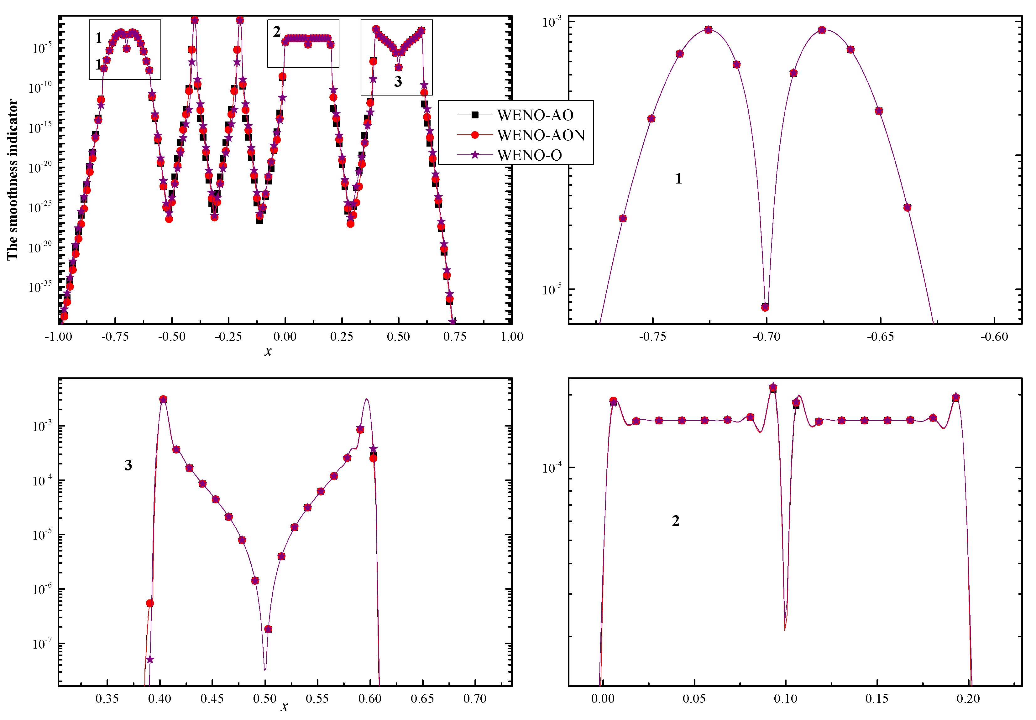
4. Analysis of the Smoothness Indicators

The observation of the Taylor series of the smoothness indicators ${\beta }^h$, ${\widehat{\beta }}^h$, and ${\overline{\beta }}^h$ reveals no difference in the order of accuracy, as will be discussed in this analysis. By using the Taylor series of $f\left(x\right)$ at $x_{i+1/2}$ for ${\beta }_0$, ${\beta }_1$ and ${\beta }_2$ (12) we have

$$\left\{\begin{array}{c}{\beta }_0=P^2{\mathsf{\Delta }x}^2-P{P}^{\prime }{\mathsf{\Delta }x}^3+[\frac{4}{3}{P^{\prime }}^2-\frac{1}{3}P{P}^{″}]{\mathsf{\Delta }x}^4+\mathrm{O}\left[{\mathsf{\Delta }x}^5\right],\\ {\beta }_1=P^2{\mathsf{\Delta }x}^2-P{P}^{\prime }{\mathsf{\Delta }x}^3+[\frac{4}{3}{P^{\prime }}^2+\frac{2}{3}P{P}^{″}]{\mathsf{\Delta }x}^4+\mathrm{O}\left[{\mathsf{\Delta }x}^5\right],\\ {\beta }_2=P^2{\mathsf{\Delta }x}^2-P{P}^{\prime }{\mathsf{\Delta }x}^3+[\frac{4}{3}{P^{\prime }}^2-\frac{1}{3}P{P}^{″}]{\mathsf{\Delta }x}^4+\mathrm{O}\left[{\mathsf{\Delta }x}^5\right].\end{array}\right.$$

(31)

For simplicity, P denotes the $f^{\prime }\left(x_{i+1/2}\right)$. Moreover, by using the Taylor series for the smoothness indicators of WENO-AO, WENO-AON and WENO-O schemes, ${\beta }^h$ (20), ${\widehat{\beta }}^h$ (21), and ${\overline{\beta }}^h$ (22), respectively, at $x_{i+1/2}$, we obtain

$$\left\{\begin{array}{c}{\beta }^h=P^2{\mathsf{\Delta }x}^2-P{P}^{\prime }{\mathsf{\Delta }x}^3+[\frac{4}{3}{P^{\prime }}^2+\frac{1}{3}P{P}^{″}]{\mathsf{\Delta }x}^4+\mathrm{O}\left[{\mathsf{\Delta }x}^5\right],\\ {\widehat{\beta }}^h=P^2{\mathsf{\Delta }x}^2-P{P}^{\prime }{\mathsf{\Delta }x}^3+\frac{4}{3}{P^{\prime }}^2{\mathsf{\Delta }x}^4+\mathrm{O}\left[{\mathsf{\Delta }x}^5\right],\\ {\overline{\beta }}^h=P^2{\mathsf{\Delta }x}^2-P{P}^{\prime }{\mathsf{\Delta }x}^3+[\frac{4}{3}{P^{\prime }}^2+\frac{4}{15}P{P}^{″}]{\mathsf{\Delta }x}^4+\mathrm{O}\left[{\mathsf{\Delta }x}^5\right].\end{array}\right.$$

(32)

As can be seen from this analysis, the three smoothness indicators, ${\beta }^h$, ${\widehat{\beta }}^h$, and ${\overline{\beta }}^h$, have the same leading and second terms which reveals that the new smoothness indicator ${\overline{\beta }}^h$ gives comparable values in smooth region of solution as the original one ${\beta }^h$.

5. Time Integration

Using method-of-lines approach, Equation (1) is estimated by the third-order three stages TVD Runge–Kutta method of [26] that is given by

$$\begin{array}{c}{u}^{\left(1\right)}=u^{\left(n\right)}+\mathsf{\Delta }tR\left(u^{\left(n\right)}\right),\hfill \\ u^{\left(2\right)}=\frac{3}{4}{u}^{\left(n\right)}+\frac{1}{4}{u}^{\left(1\right)}+\frac{1}{4}\mathsf{\Delta }tR{u}^{\left(1\right)},\hfill \\ u^{(n+1)}=\frac{1}{3}{u}^{\left(n\right)}+\frac{2}{3}{u}^{\left(2\right)}+\frac{2}{3}\mathsf{\Delta }tR\left(u^{\left(2\right)}\right),\hfill \end{array}$$

(33)

with $\mathsf{\Delta }t$ and n are the time step and time level, respectively.

6. Numerical Experiments

To demonstrate the accuracy and convergence rate of the devised WENO-O scheme, eight test cases are studied and shown. To perform a fair comparison, the original WENO-AO, WENO-AON, WENO-Z, and WENO-JS schemes are adopted to assess the performance of the new WENO-O scheme. To calculate the errors in $L_1-,L_{\infty }-$ norms the exact solution ${\overline{u}}_i^{exact}$ is compared with the numerical solution ${\overline{u}}_i$ with, using

$$\begin{array}{c}{∥error∥}_1=\mathsf{\Delta }x{\displaystyle \sum _{i=1}^N} \left|{\overline{u}}_i-{\overline{u}}_i^{exact}\right|,\hfill \\ {∥error∥}_{\infty }=max\left(\left|{\overline{u}}_i-{\overline{u}}_i^{exact}\right|\right),\hfill \end{array}$$

(34)

where N is the cell number.

6.1. Scalar Equation

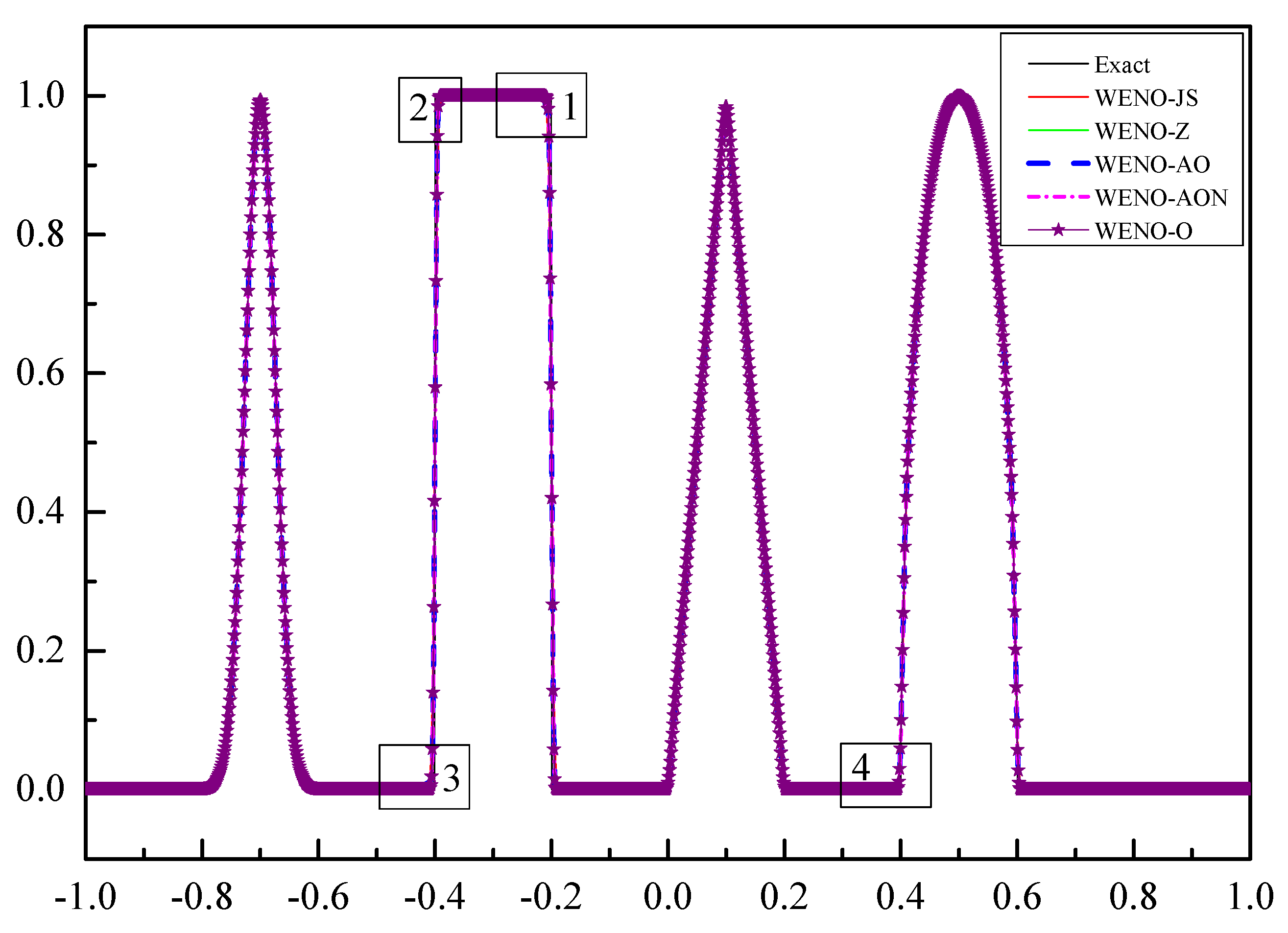
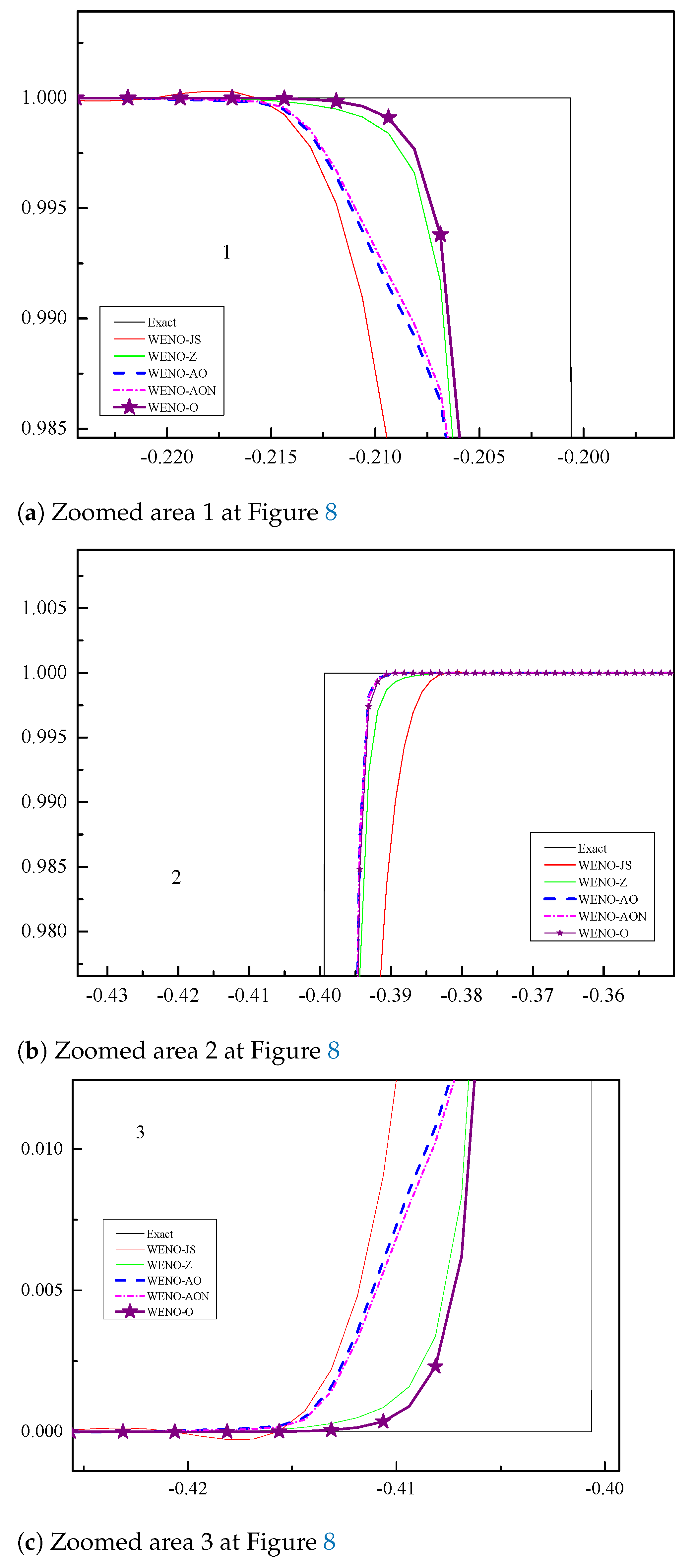
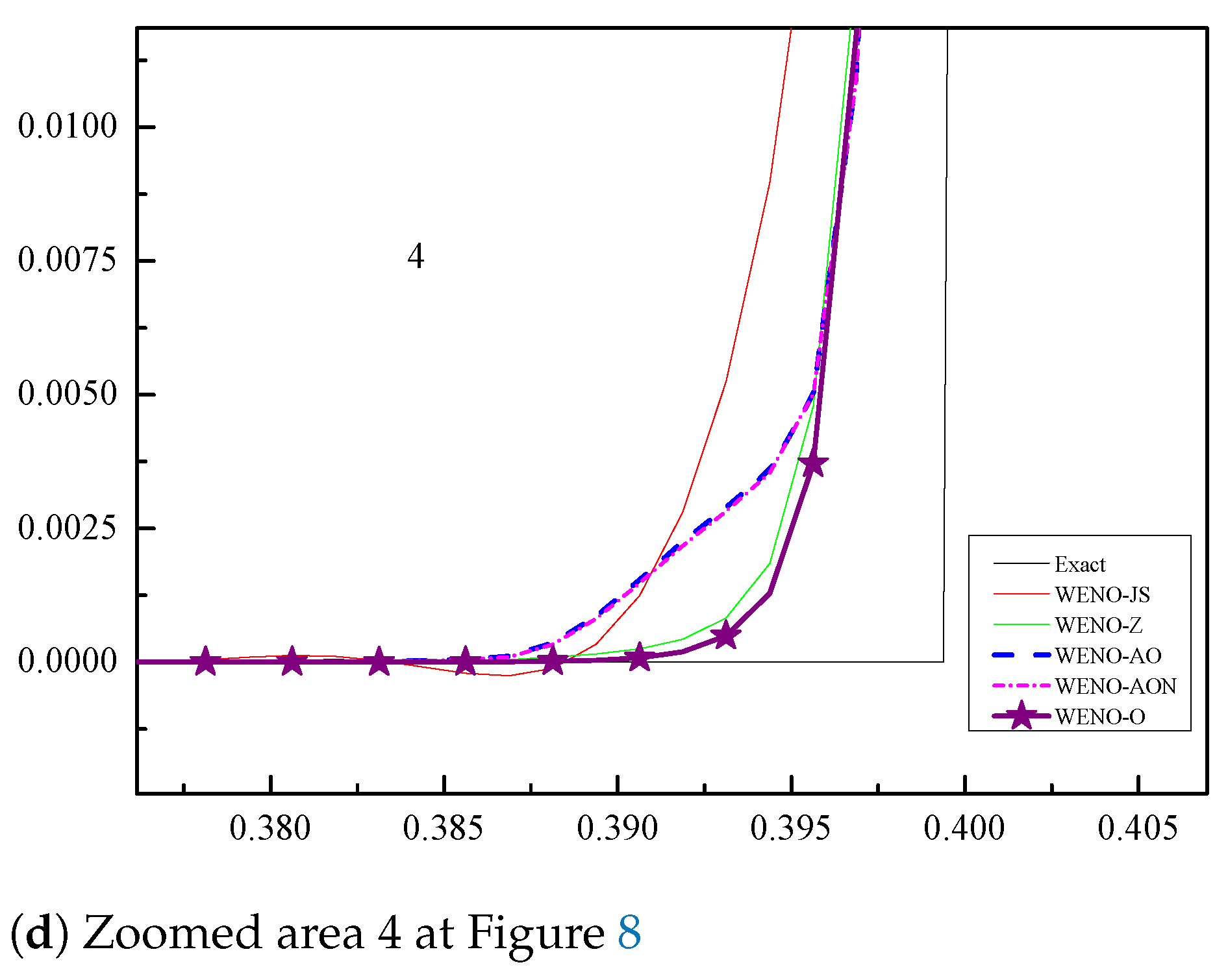
6.1.1. Example (1)—Linear Advection of Sinusoidal Profiles

On the 1-D periodic domain $x\in (-1,1)$, the scalar advection equation is solved

$$u_t+u_x=0,$$

(35)

with initial condition

$$u(x,0)=sin\left(\pi x\right),x\in (-1,1).$$

The numerical computations were run to a final time of $t=10$ with $CFL={\left(\mathsf{\Delta }x\right)}^{2/3}$. This case was used to test the convergence rate of the new scheme WENO-O because, as time evolves, the solution is always smooth. For all considered fifth-order WENO schemes, $L_1$ -norm errors, $L_{\infty }$ -norm errors, computational time and the accuracy are presented in

Table 3. The sine wave advection test accuracy (Section 6.1.1) with WENO-JS, WENO-AO, WENO-Z, WENO-AON and WENO-O schemes.

Method	N	40	80	160	320	640
	$L_1$-norm error	4.6300 × 10${}^{-4}$	1.4500 × 10${}^{-5}$	4.5100 × 10${}^{-7}$	1.4100 × 10${}^{-8}$	4.3700 × 10${}^{-10}$
WENO-JS	$L_{\infty }$-norm error	3.9447 × 10${}^{-4}$	1.3153 × 10${}^{-5}$	4.1205 × 10${}^{-7}$	1.2966 × 10${}^{-8}$	3.7797 × 10${}^{-10}$
	CPU time	0.0737	0.2244	0.7555	2.8856	11.9590
	$L_1$ accuracy	-	5.00096	5.00143	5.00257	5.00925
	$L_1$-norm error	7.9900 × 10${}^{-5}$	2.5000 × 10${}^{-6}$	7.8000 × 10${}^{-8}$	2.4400 × 10${}^{-9}$	7.6200 × 10${}^{-11}$
WENO-Z	$L_{\infty }$-norm error	6.3800 × 10${}^{-5}$	1.9714 × 10${}^{-6}$	6.1381 × 10${}^{-8}$	1.9160 × 10${}^{-9}$	5.9857 × 10${}^{-11}$
	CPU time	0.07316	0.22302	0.7488	2.8570	12.1060
	$L_1$ accuracy	-	5.00101	4.99947	4.99982	4.99964
	$L_1$-norm error	7.9644 × 10${}^{-5}$	2.4949 × 10${}^{-6}$	7.8014 × 10${}^{-8}$	2.4383 × 10${}^{-9}$	7.6215 × 10${}^{-11}$
WENO-AO	$L_{\infty }$-norm error	6.2539 × 10${}^{-5}$	1.9595 × 10${}^{-6}$	6.1272 × 10${}^{-8}$	1.9151 × 10${}^{-9}$	5.9855 × 10${}^{-11}$
	CPU time	0.0936	0.3021	1.0136	3.8675	16.2850
	$L_1$ accuracy	-	4.99651	4.99911	4.99979	4.99966
	$L_1$-norm error	7.9644 × 10${}^{-5}$	2.4949 × 10${}^{-6}$	7.8014 × 10${}^{-8}$	2.4383 × 10${}^{-9}$	7.6214 × 10${}^{-11}$
WENO-AON	$L_{\infty }$-norm error	6.2540 × 10${}^{-5}$	1.9595 × 10${}^{-6}$	6.1272 × 10${}^{-8}$	1.9150 × 10${}^{-9}$	5.9843 × 10${}^{-11}$
	CPU time	0.0853	0.2628	0.8998	3.5138	14.5450
	$L_1$ accuracy	-	4.99651	4.99911	4.99979	4.99968
	$L_1$-norm error	7.9645 × 10${}^{-5}$	2.4949 × 10${}^{-6}$	7.8014 × 10${}^{-8}$	2.4383 × 10${}^{-9}$	7.6215 × 10${}^{-11}$
WENO-O	$L_{\infty }$-norm error	6.2573 × 10${}^{-5}$	1.9595 × 10${}^{-6}$	6.1272 × 10${}^{-8}$	1.9151 × 10${}^{-9}$	5.9863 × 10${}^{-11}$
	CPU time	0.0822	0.2482	0.8219	3.1722	13.4120
	$L_1$ accuracy	-	4.99653	4.99911	4.99979	4.99966

with different mesh numbers. In this table, it is shown that all the methods reach their design accuracies. On comparing the new WENO scheme (WEON-O) with both adaptive order schemes (WENO-AO and WENO-AON), for the same mesh, the new scheme exhibits less computational time which is good to see for decreasing the adaptive order schemes’ computational cost. Furthermore, the proposed WENO-O scheme presents similar efficiency as both adaptive order schemes, as can be seen from Figure 2 and Figure 3.

6.1.2. Example (2)—Non-Linear Burgers Equation in One Dimension

On the one-dimensional periodic domain, we use the non-linear Burgers equation

$$u_t+{(u^2/2)}_x=0,x\in (0,2),$$

(36)

with initial condition

$$u(x,0)=\left\{\begin{array}{c}0,\mathrm{if}x\in (0.5,1),\\ -4,\mathrm{if}x\in (1,2),\\ 1,\mathrm{otherwise}.\end{array}\right.$$

We run numerical simulations to a final time of $t=1$ with $CFL=0.1$ on different uniform mesh numbers for all considered WENO schemes as described in Example 1 (Section 6.1.1). The accuracy results along with $L_1$ -norm errors and computational time are given in

Table 4. The non-linear Burgers equation accuracy (Section 6.1.2) in 1-D with WENO-JS, WENO-AO, WENO-Z, WENO-AON and WENO-O schemes.

Method	N	100	200	400	800	1600
	$L_1$-norm error	10.5320 × 10${}^{-2}$	4.9560 × 10${}^{-2}$	1.8770 × 10${}^{-2}$	9.7500 × 10${}^{-3}$	6.1100 × 10${}^{-3}$
WENO-JS	CPU time	0.0884	0.1893	0.4628	1.3257	4.1040
	$L_1$ accuracy	-	1.08739	1.40112	0.94452	0.67477
	$L_1$-norm error	8.9590 × 10${}^{-2}$	4.0470 × 10${}^{-2}$	1.5630 × 10${}^{-2}$	8.0900 × 10${}^{-3}$	5.3100 × 10${}^{-3}$
WENO-Z	CPU time	0.0918	0.1978	0.4818	1.3818	4.2026
	$L_1$ accuracy	-	1.14656	1.37206	0.95128	0.60665
	$L_1$-norm error	9.5970 × 10${}^{-2}$	4.328 × 10${}^{-2}$	1.6460 × 10${}^{-2}$	8.5900 × 10${}^{-3}$	5.5400 × 10${}^{-3}$
WENO-AO	CPU time	0.1210	0.2654	0.6338	1.8035	7.7902
	$L_1$ accuracy	-	1.14886	1.39521	0.93783	0.63237
	$L_1$-norm error	8.4530 × 10${}^{-2}$	3.9110 × 10${}^{-2}$	1.5450 × 10${}^{-2}$	7.8600 × 10${}^{-3}$	5.1900 × 10${}^{-3}$
WENO-AON	CPU time	0.1061	0.2305	0.5772	1.6001	6.7917
	$L_1$ accuracy	-	1.11204	1.33956	0.97565	0.5972
	$L_1$-norm error	9.1120 × 10${}^{-2}$	4.067 × 10${}^{-2}$	1.5680 × 10${}^{-2}$	8.1000 × 10${}^{-3}$	5.3000 × 10${}^{-3}$
WENO-O	CPU time	0.1025	0.2170	0.5269	1.5128	4.5968
	$L_1$ accuracy	-	1.16402	1.3749	0.95213	0.61221

. We see that our WENO-O scheme is somewhat better than WENO-AO scheme in terms of computational time. Moreover, the efficiency of the proposed method is also better than adaptive order scheme WENO-AO as can be seen from Figure 4 and Figure 5. However, the new WENO-O scheme gives more accurate solution, on the same mesh, than WENO-AO scheme (see Figure 5). Moreover, the values of smoothness indicators ${\overline{\beta }}^h$, ${\beta }^h$, and ${\widehat{\beta }}^h$ of WENO-O, WENO-AO, and WENO-AON schemes, respectively, are displayed in Figure 6 in which the value of smoothness indicator of WENO-O scheme showed closer results to that of WENO-AON and WENO-AO schemes.

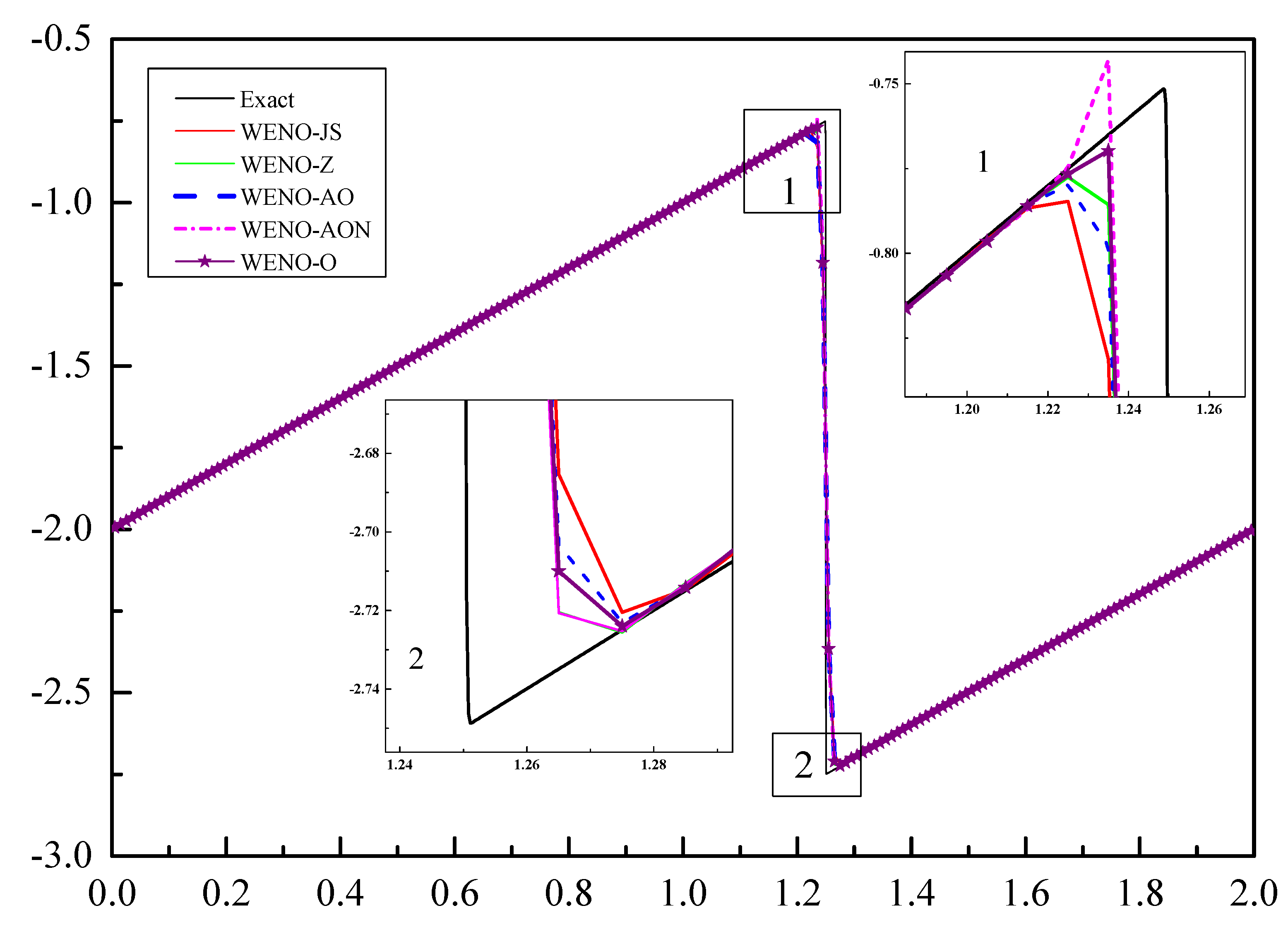
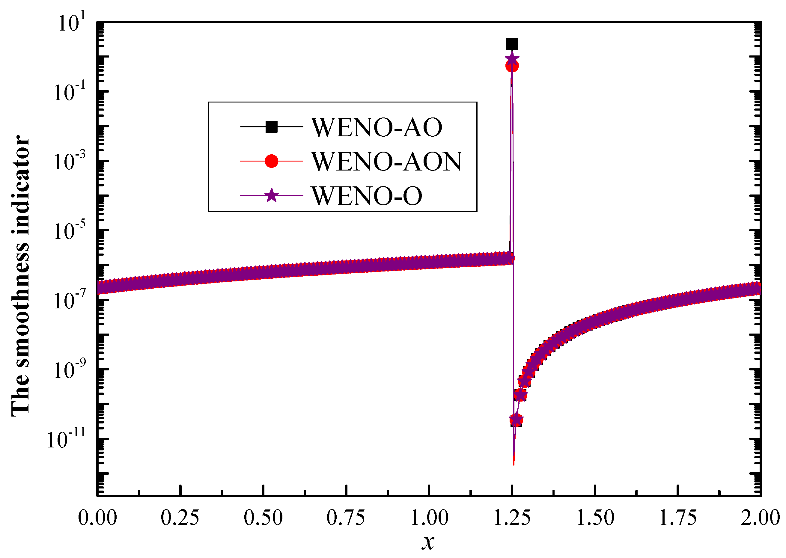
6.1.3. Example (3)—The Scalar Advection Test Problem

The 1-D periodic domain $x\in (-1,1)$ is considered to solve the scalar advection equation

$$u_t+u_x=0,x\in [-1,1],$$

with initial condition

$$u(x,0)=\left\{\begin{array}{l} \frac{1}{6}[F(x,\beta ,z-\delta )+F(x,\beta ,z+\delta )+4F(x,\beta ,z)],\mathrm{if}x\in [-0.8,-0.6],\\ 1,\mathrm{if}x\in [-0.4,-0.2],\\ 1-\left|10(x-0.1)\right|,\mathrm{if}x\in [0,0.2],\\ \frac{1}{6}[G(x,\alpha ,a-\delta )+G(x,\alpha ,a+\delta )+4F(x,\alpha ,a)],\mathrm{if}x\in [0.4,0.6],\\ \hspace{1em}\hspace{1em} 0,\mathrm{otherwise},\end{array}\right.$$

(37)

where

$$F(x,\alpha ,a)=\sqrt{max(1-{\alpha }^2{(x-a)}^2,0)},F(x,\beta ,z)=e^{-\beta {(x-z)}^2},$$

and the constants are $\delta =0.005,$ $\alpha =10,$ $z=-0.7,$ $a=0.5$ and $\beta =log2/36{\delta }^2$. This test case is conducted to assess the ability of the devised WENO-O scheme to resolve rich constructions of the solution that contains a smooth but narrow combination of a square wave, Gaussian, half ellipse, and sharp triangle wave. The simulations are performed at $t=10$ and $CFL=0.1$ with different meshes. The accuracy of considered fifth-order WENO schemes is presented in

Table 5. The accuracy of scalar advection test of Example 3 (Section 6.1.3) in one dimension with WENO-AO, WENO-AON, WENO-JS, WENO-Z and WENO-O schemes.

Method	N	100	200	400	800	1600
	$L_1$-norm error	14.5820 × 10${}^{-2}$	6.2810 × 10${}^{-2}$	2.8020 × 10${}^{-2}$	1.4020 × 10${}^{-2}$	7.4000 × 10${}^{-3}$
WENO-JS	CPU time	0.0567	0.1167	0.2670	0.7877	2.2937
	$L_1$ accuracy	-	1.21512	1.16454	0.99897	0.92189
	$L_1$-norm error	10.3540 × 10${}^{-2}$	4.4910 × 10${}^{-2}$	2.0940 × 10${}^{-2}$	1.0560 × 10${}^{-2}$	5.5200 × 10${}^{-3}$
WENO-Z	CPU time	0.0555	0.1193	0.3035	0.7751	2.3831
	$L_1$ accuracy	-	1.20508	1.10078	0.98765	0.93587
	$L_1$-norm error	9.7320 × 10${}^{-2}$	4.3500 × 10${}^{-2}$	2.0000 × 10${}^{-2}$	1.0130 × 10${}^{-2}$	5.3400 × 10${}^{-3}$
WENO-AO	CPU time	0.0758	0.1596	0.3838	1.1061	4.3390
	$L_1$ accuracy	-	1.16172	1.12102	0.98137	0.92372
	$L_1$-norm error	9.4160 × 10${}^{-2}$	4.2970 × 10${}^{-2}$	1.9850 × 10${}^{-2}$	1.0100 × 10${}^{-2}$	5.3200 × 10${}^{-3}$
WENO-AON	CPU time	0.0686	0.1403	0.3382	0.9420	3.8419
	$L_1$ accuracy	-	1.13178	1.11419	0.97764	0.922
	$L_1$-norm error	10.0930 × 10${}^{-2}$	4.4060 × 10${}^{-2}$	2.0280 × 10${}^{-2}$	1.0200 × 10${}^{-2}$	5.3300 × 10${}^{-3}$
WENO-O	CPU time	0.0602	0.1281	0.3436	0.8360	2.5197
	$L_1$ accuracy	-	1.19581	1.11941	0.99149	0.93636

, in which $L_1$-norm errors, computational time and convergence rates display that the solution of the new scheme is comparable to the adaptive order WENO schemes. Moreover, WENO-O scheme reduces the computational cost of the adaptive order schemes; this also can be observed from Figure 7. In addition, the results are plotted in Figure 8 for 1600 mesh points and the close view of some locations is presented in Figure 9. It could be observed that the devised scheme exhibited better solution than other schemes and then higher efficiency. Moreover, convergence rates of all schemes dropped to first order from fifth order, due to discontinuities in the solution. Furthermore, the values of smoothness indicator ${\overline{\beta }}^h$, ${\beta }^h$, and ${\widehat{\beta }}^h$ of WENO-O, WENO-AO, and WENO-AON schemes, respectively, are demonstrated in Figure 10 in which the value of new smoothness indicator of WENO-O scheme showed closer results to that of WENO-AON and WENO-AO schemes.

6.2. One-Dimensional Euler Equations

The three well-known cases governed by the 1-D Euler Equation (38) are examined in Examples 4–6.

$$\frac{\partial \mathbf{U}}{\partial t}+\frac{\partial \mathbf{F}\left(\mathbf{U}\right)}{\partial x}=0,$$

(38)

here $\mathbf{U}$ and $\mathbf{F}$ represent conservative vector and convective flux in x direction, respectively, which are

$$\begin{array}{c}\mathbf{U}={(\rho ,\rho u,E)}^T,\hfill \\ \mathbf{F}\left(\mathbf{U}\right)={(\rho u,\rho u^2+p,u(E+p))}^T,\hfill \end{array}$$

where $E,p,u$ and $\rho$ denote the total energy, pressure, velocity component in x direction and the density, respectively. The pressure is calculated by

$$p=(\gamma -1)(E-\frac{1}{2}\rho u^2),$$

where $\gamma$ denotes the specific heat ratio ($\gamma =1.4$ for all considered cases).

6.2.1. Example (4)—The Lax Test Problem

To assess the capability of the devised WENO-O scheme to capture relatively strong shock, the Lax problem is used [27]. The initial conditions are

$$(\rho ,u,p)=\left\{\begin{array}{c}(0.445,0.698,3.528),\mathrm{if}x<0,\\ (0.5,0,0.571),\mathrm{if}x>0.\end{array}\right.$$

(39)

All simulations are performed on uniform grid composed of four different meshes ($x\in [-4,4]$) at non-dimensional final time of $t=1.3$ and $CFL=0.95$. At different uniform meshes, the accuracy of considered fifth-order WENO schemes including the proposed WENO-O scheme are summarized in

Table 6. The accuracy of Lax’s test of Example 4 (Section 6.2.1) in one dimension with WENO-AO, WENO-AON, WENO-JS, WENO-Z and WENO-O schemes.

Method	N	100	200	400	800
	$L_1$-norm error	2.2053 × 10${}^{-1}$	1.2080 × 10${}^{-1}$	5.8170 × 10${}^{-2}$	3.2700 × 10${}^{-2}$
WENO-JS	CPU time	0.5005	1.6318	6.4533	25.3660
	$L_1$ accuracy	-	0.86835	1.05427	0.83098
	$L_1$-norm error	1.7743 × 10${}^{-1}$	9.6730 × 10${}^{-2}$	4.4950 × 10${}^{-2}$	2.5640 × 10${}^{-2}$
WENO-Z	CPU time	0.5018	1.6433	6.2886	25.2070
	$L_1$ accuracy	-	0.87521	1.10564	0.80992
	$L_1$-norm error	1.8416 × 10${}^{-1}$	9.9480 × 10${}^{-2}$	4.5600 × 10${}^{-2}$	2.6200 × 10${}^{-2}$
WENO-AO	CPU time	0.5849	1.7990	7.3039	29.1650
	$L_1$ accuracy	-	0.88848	1.12442	0.79821
	$L_1$-norm error	1.7110 × 10${}^{-1}$	9.2890 × 10${}^{-2}$	4.3090 × 10${}^{-2}$	2.4750 × 10${}^{-2}$
WENO-AON	CPU time	0.5442	1.8045	7.0549	28.2850
	$L_1$ accuracy	-	0.88124	1.10817	0.79992
	$L_1$-norm error	1.7887 × 10${}^{-1}$	9.6990 × 10${}^{-2}$	4.4730 × 10${}^{-2}$	2.5580 × 10${}^{-2}$
WENO-O	CPU time	0.5149	1.7442	6.8033	27.3540
	$L_1$ accuracy	-	0.88300	1.11659	0.80623

and Figure 11; however, our scheme reveals less $L_1$-error norm with the same grids than WENO-AO scheme. Moreover, it gives less computational time than that of the original WENO-AON and WENO-AO schemes. Moreover, the results exhibited that the new WENO-O scheme provides correct solutions and good resolution to the shock wave as accurate as adaptive order WENO schemes (WENO-AON and WENO-AO schemes) and the contact discontinuity can be resolved sharply as illustrated in Figure 12 and Figure 13.

6.2.2. Example (5)—The Sod Test Problem

The 1-D Euler Equation (38) were solved on $x\in [-5,5]$ using

$$(\rho ,u,p)= \left\{\begin{array}{c}(1,0,1),\mathrm{if}x<0,\\ (0.125,0,0.1),\mathrm{if}x>0.\end{array}\right.$$

(40)

This Riemann problem [28] that contains contact discontinuity, shock, and rarefaction waves is simulated at $t=2$ and $CFL=0.1$ with different uniform meshes. The results of the $L_1$ error norms, convergence rates and computational time are summarized in

Table 7. The accuracy of Sod’s test of Example 5 (Section 6.2.2) in one dimension with WENO-AO, WENO-AON, WENO-JS, WENO-Z and WENO-O schemes.

Method	N	80	150	320	640
	$L_1$-norm error	10.217 × 10${}^{-2}$	5.2620 × 10${}^{-2}$	2.7250 × 10${}^{-2}$	1.4250 × 10${}^{-2}$
WENO-JS	CPU time	1.4147	5.2543	21.3190	85.1990
	$L_1$ accuracy	-	0.95729	0.94936	0.93529
	$L_1$-norm error	8.7670 × 10${}^{-2}$	4.4480 × 10${}^{-2}$	2.2810 × 10${}^{-2}$	1.1930 × 10${}^{-2}$
WENO-Z	CPU time	1.4665	5.4114	21.7280	87.2130
	$L_1$ accuracy	-	0.97893	0.96349	0.93507
	$L_1$-norm error	8.8940 × 10${}^{-2}$	4.4880 × 10${}^{-2}$	2.2870 × 10${}^{-2}$	1.1910 × 10${}^{-2}$
WENO-AO	CPU time	1.7262	6.3594	25.7530	103
	$L_1$ accuracy	-	0.98676	0.97262	0.94128
	$L_1$-norm error	8.3130 × 10${}^{-2}$	4.2260 × 10${}^{-2}$	2.1720 × 10${}^{-2}$	1.1420 × 10${}^{-2}$
WENO-AON	CPU time	1.5325	5.8208	23.577	93.4990
	$L_1$ accuracy	-	0.97608	0.96027	0.92746
	$L_1$-norm error	8.6990 × 10${}^{-2}$	4.4230 × 10${}^{-2}$	2.2690 × 10${}^{-2}$	1.1870 × 10${}^{-2}$
WENO-O	CPU time	1.5241	5.7645	23.1690	92.6200
	$L_1$ accuracy	-	0.97582	0.96297	0.93474

and Figure 14. A similar observation as in Example 4 (Section 6.2.1) can be concluded from this example. The efficiency of the devised scheme for predicting the solution of Sod’s problem is illustrated in Figure 15 and Figure 16. Thus, the devised WENO-O scheme predicts the contact discontinuity, shock, and rarefaction waves as accurate as adaptive order and WENO-Z schemes and better than WENO-JS scheme.

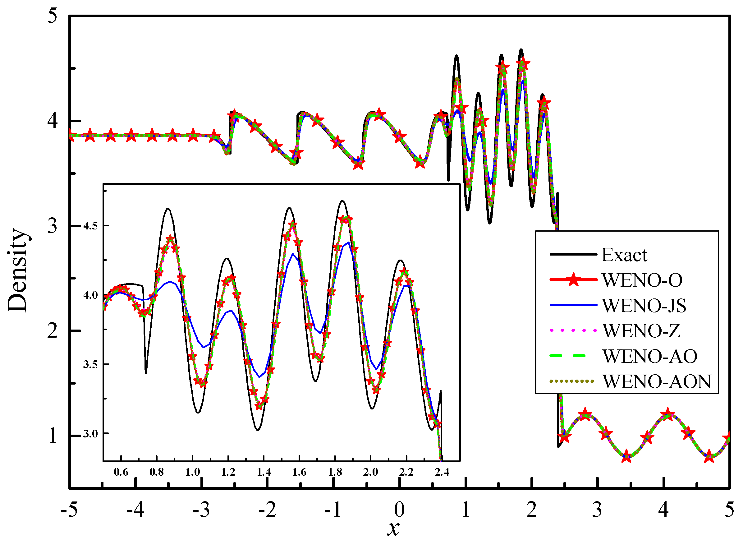
6.2.3. Example (6)—The Shu–Osher Problem

The 1-D Euler Equation (38) on $x\in [-5,5]$ are considered with

$$(\rho ,u,p)(x,0)=\left\{\begin{array}{c}(27/7,4\sqrt{35}/9,31/3),\mathrm{if}x<-4,\\ (1+0.2sin(5x),0.0,1.0),\mathrm{if}x>-4.\end{array}\right.$$

(41)

The shock entropy wave interaction problem of Shu–Osher [29] is also adopted to test the new WENO-O scheme. The numerical solutions are run with CFL number $0.1$ to final time of $t=1.8$. Since the exact solution is unavailable, the solution of WENO-AO scheme that obtained over mesh size of 6400 is adopted as the reference solution. From Figure 17 and Figure 18, it shows the similar conclusion as in Example 4 (Section 6.2.1) for both accuracy and efficiency of proposed WENO-O scheme.

6.3. Two-Dimensional Euler Equations

To further test the proposed WENO-O scheme, two test cases for two-dimensional coordinates (2-D) are simulated; two of which are two-dimensional Riemann problems along with double-Mach reflection of strong shock. Therefore, the 2-D Euler Equation (42) are used in this work.

$$\frac{\partial \mathbf{U}}{\partial t}+\frac{\partial \mathbf{F}\left(\mathbf{U}\right)}{\partial x}+\frac{\partial \mathbf{G}\left(\mathbf{U}\right)}{\partial y}=0,$$

(42)

here $\mathbf{U}$ is the conservative vector, $\mathbf{F}$ and $\mathbf{G}$ are the convective fluxes in x and y directions, respectively, which are

$$\begin{array}{c}\mathbf{U}={(\rho ,\rho u,\rho v,E)}^T,\hfill \\ \mathbf{F}\left(\mathbf{U}\right)={(\rho u,\rho u^2+p,\rho uv,u(E+p))}^T,\hfill \\ \mathbf{G}\left(\mathbf{U}\right)={(\rho v,\rho uv,\rho v^2+p,v(E+p))}^T,\hfill \end{array}$$

with $E,p,u,v,p$ and $\rho$ denote the total energy, pressure, velocity components in x and y directions and density, respectively. The pressure is calculated by

$$p=(\gamma -1)(E-\frac{1}{2}\rho (u^2+v^2)),$$

and $\gamma$ denotes the specific heat ratio ($\gamma =1.4$ for all considered cases).

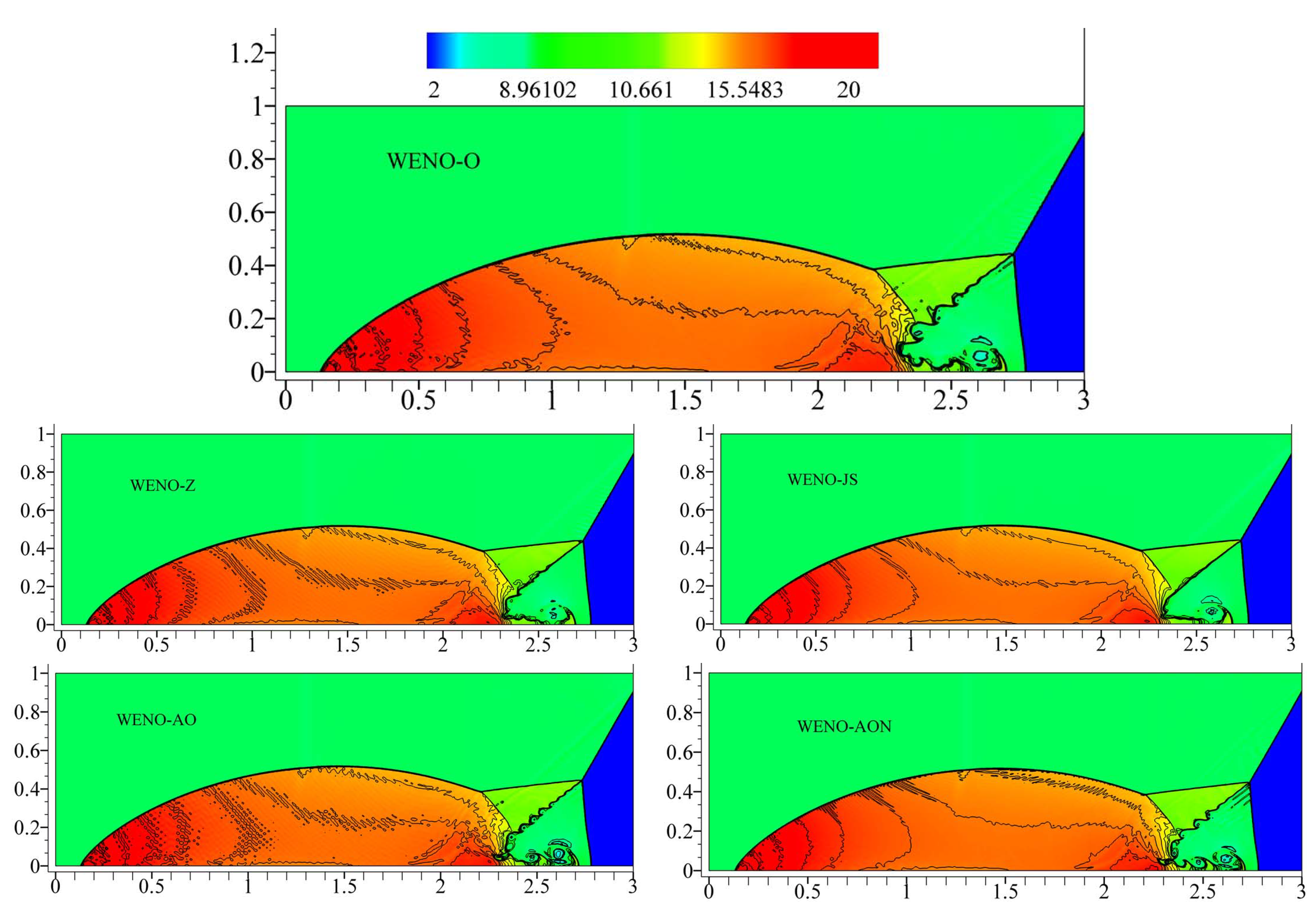
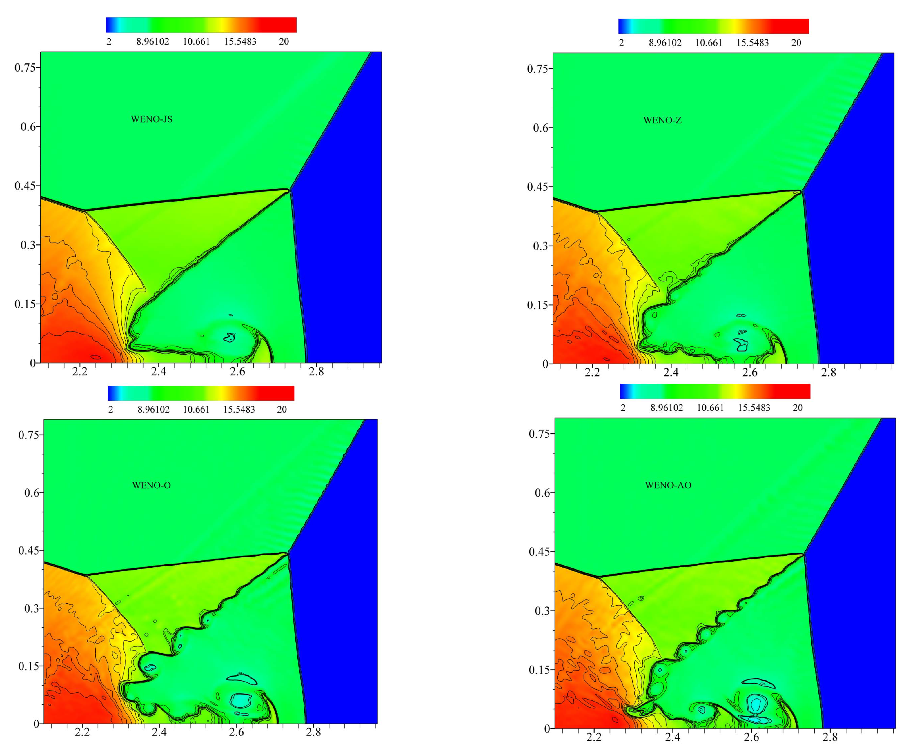
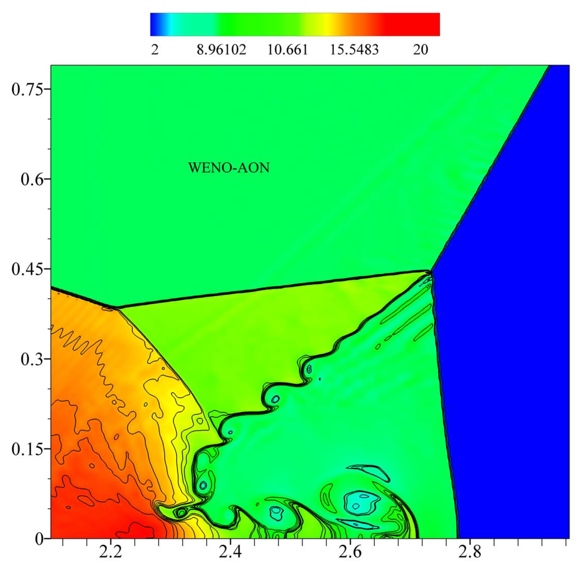
6.3.1. Example (7)—Double-Mach Reflection of Strong Shock

Woodward and Colella [30] have proposed the well-known 2-D Double-Mach shock reflection test case that had been taken extensively to assess high resolution schemes. In this case, a strong vertical shock moves horizontally into a wedge that is inclined with some angle. The considered WENO schemes were used to simulate a 2-D computational domain of $[0,4]\times [0,1]$ whereas the reflective wall lies on the bottom of the computational domain for $1/6\le x\le 4$. In the beginning, a right-moving Mach 10 shock is positioned at $x=1/6,$ $y=0$ and creates an angle 60° with the x-axis. More details can be found elsewhere [30]. We consider the 2-D Euler Equation (42) with initial conditions

$${(\rho ,u,v,p)}_{t=0}=\left\{\begin{array}{c}(8.0,8.25cos(\pi /6),-8.25sin(\pi /6),116.5),\mathrm{if}x<\frac{1}{6}+\frac{y}{\sqrt{3}},\\ (1.4,0.0,0.0,1.0),\mathrm{if}x\ge \frac{1}{6}+\frac{y}{\sqrt{3}}.\end{array}\right.$$

(43)

Numerical results of the density achieved from the proposed WENO-O scheme and other considered fifth-order WENO schemes at time $t=0.2$, CFL = 0.475, and 1600 × 400 points are demonstrated in Figure 19 and Figure 20. On comparing the new scheme WENO-O with other schemes, it can be observed that our scheme reveals a much high resolution around the blown-up region with complicated structures than WENO-Z and WENO-JS schemes; and similar to WENO-AO and WENO-AON schemes. Moreover, it can be observed that at the end of the slip line and the wall jet, the rendering of small vortices becomes clear for adaptive order schemes including the WENO-O scheme (see Figure 20). In addition, the CPU time (s) of new WENO-O, WENO-AON, and WENO-AO schemes were 35,094.84, 36,105.65 and 37,536.94, respectively, which confirms that the proposed scheme decreases the computational cost of the original scheme.

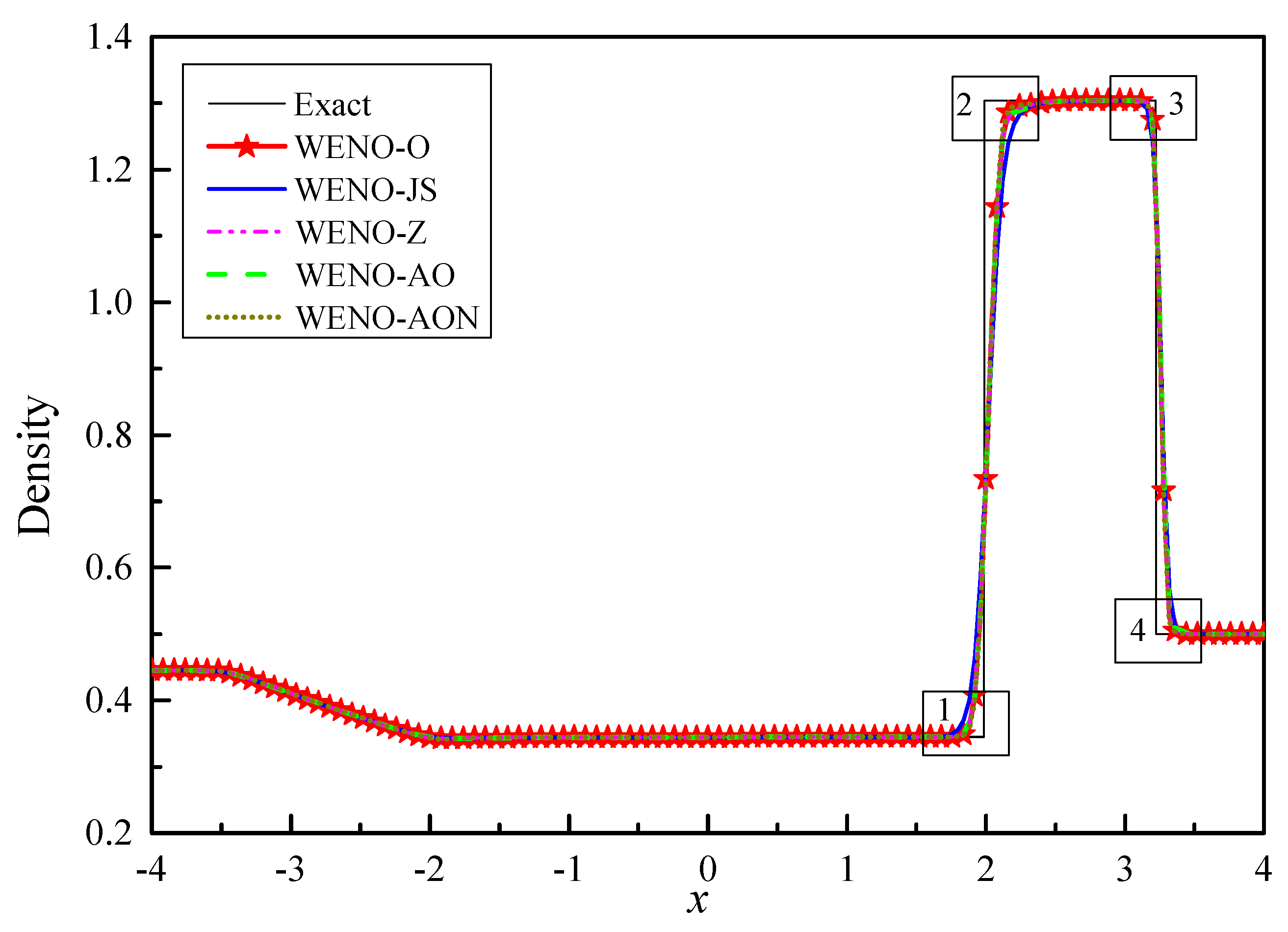
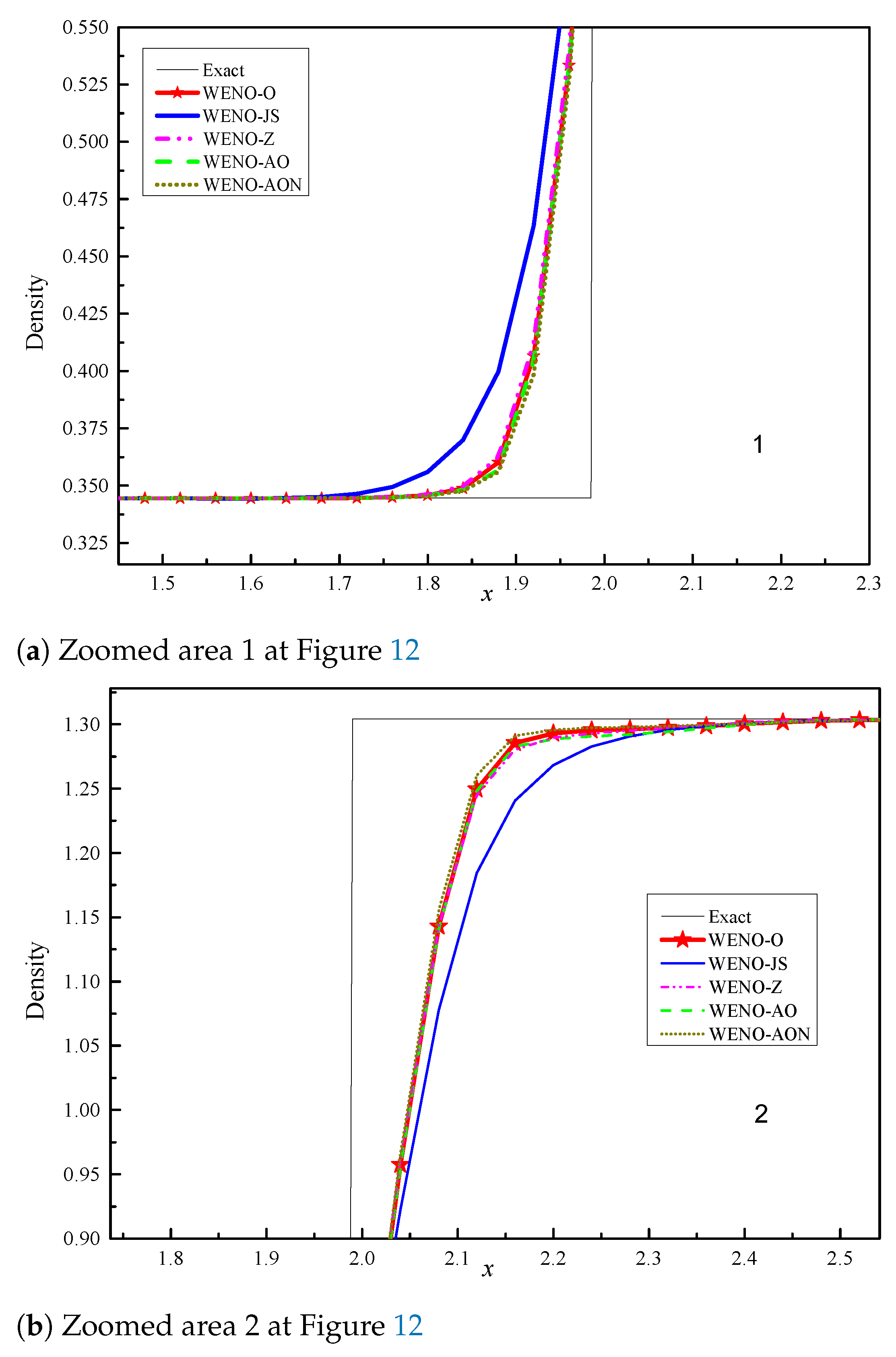
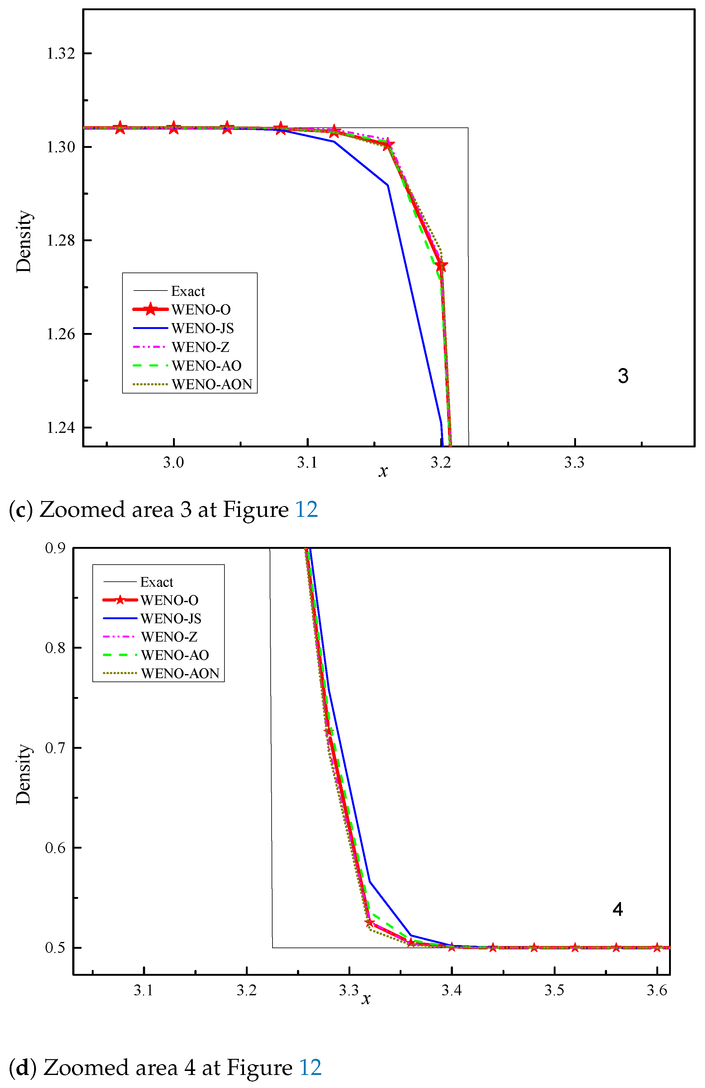
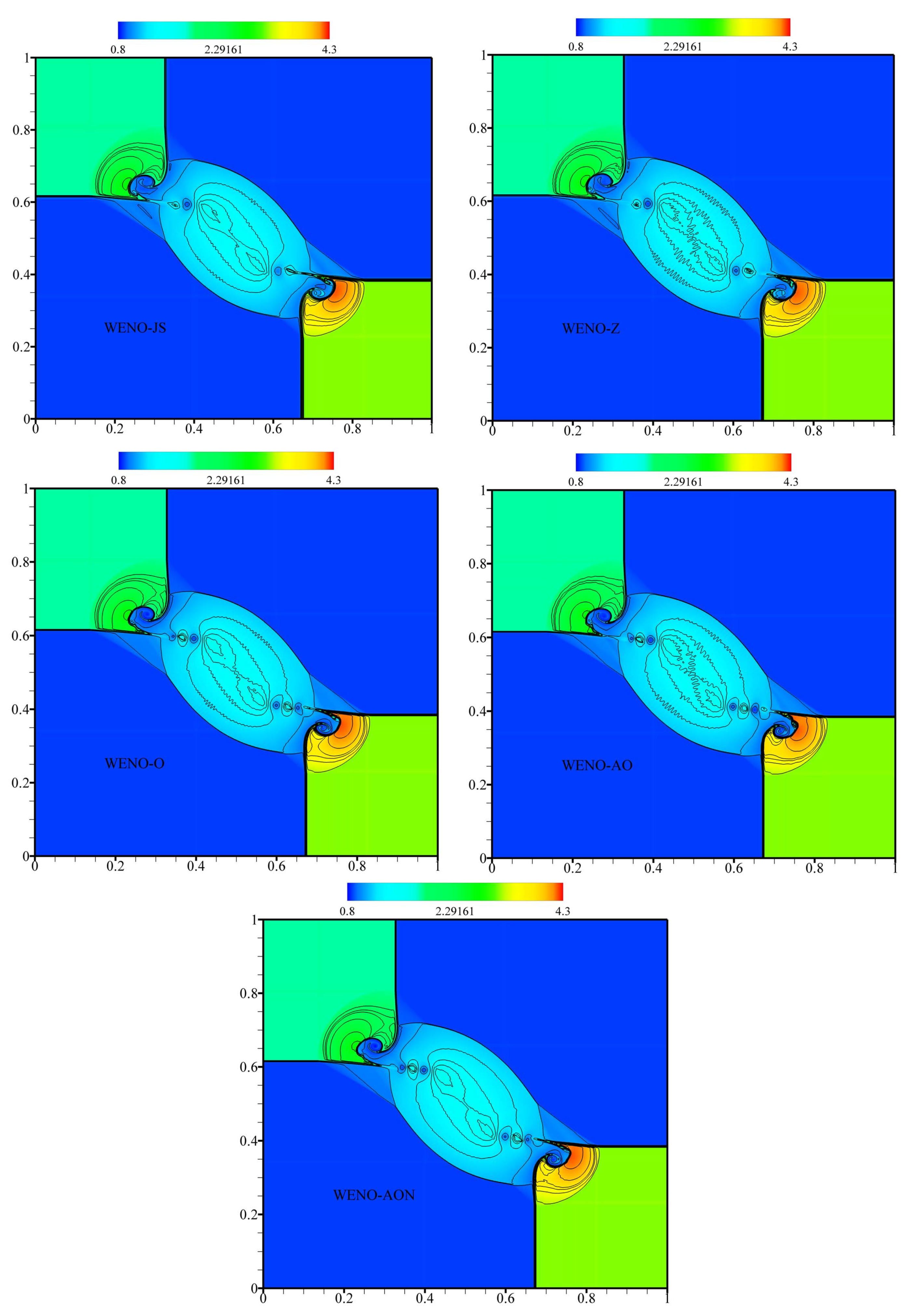
6.3.2. Example (8)—2-D Riemann initial data (Lax-Liu)

To assess the capability of the devised WENO-O scheme for different structures, such as contact discontinuities, reflection shocks and instability interfaces, a 2-D Riemann test case proposed by [31] is adopted. We consider the 2-D Euler Equation (42) with initial conditions

$$\begin{array}{c}\hfill {(\rho ,u,v,p)}_{t=0}=\left\{\begin{array}{c}(1,-0.75,-0.5,1),\mathrm{if}0.5\le x\le 1,0.5\le y\le 1,\\ (2,-0.75,0.5,1),\mathrm{if}0\le x\le 0.5,0.5\le y\le 1,\\ (1,0.75,0.5,1),\mathrm{if}0\le x\le 0.5,0\le y\le 0.5,\\ (3,0.75,-0.5,1),\mathrm{if}0.5\le x\le 1,0\le y\le 0.5.\end{array}\right.\end{array}$$

(44)

The simulations were run to a final time of 0.23 with $CFL=0.6$ in a computational domain of $[0,1]\times [0,1]$ that is divided into four quadrants by two lines $x=0.5$ and $y=0.5$ with mesh grid of size 800 × 800. This test case revealed that the new WENO-O scheme resolves the contact discontinuity and shock waves very well as displayed in Figure 21. Moreover, WENO-O scheme has also decreased the computational cost of WENO-AO scheme where WENO-O, WENO-AON, and WENO-AO schemes cost CPU time of 9120.62 s, 9526.09 s, and 9788.74 s, respectively.

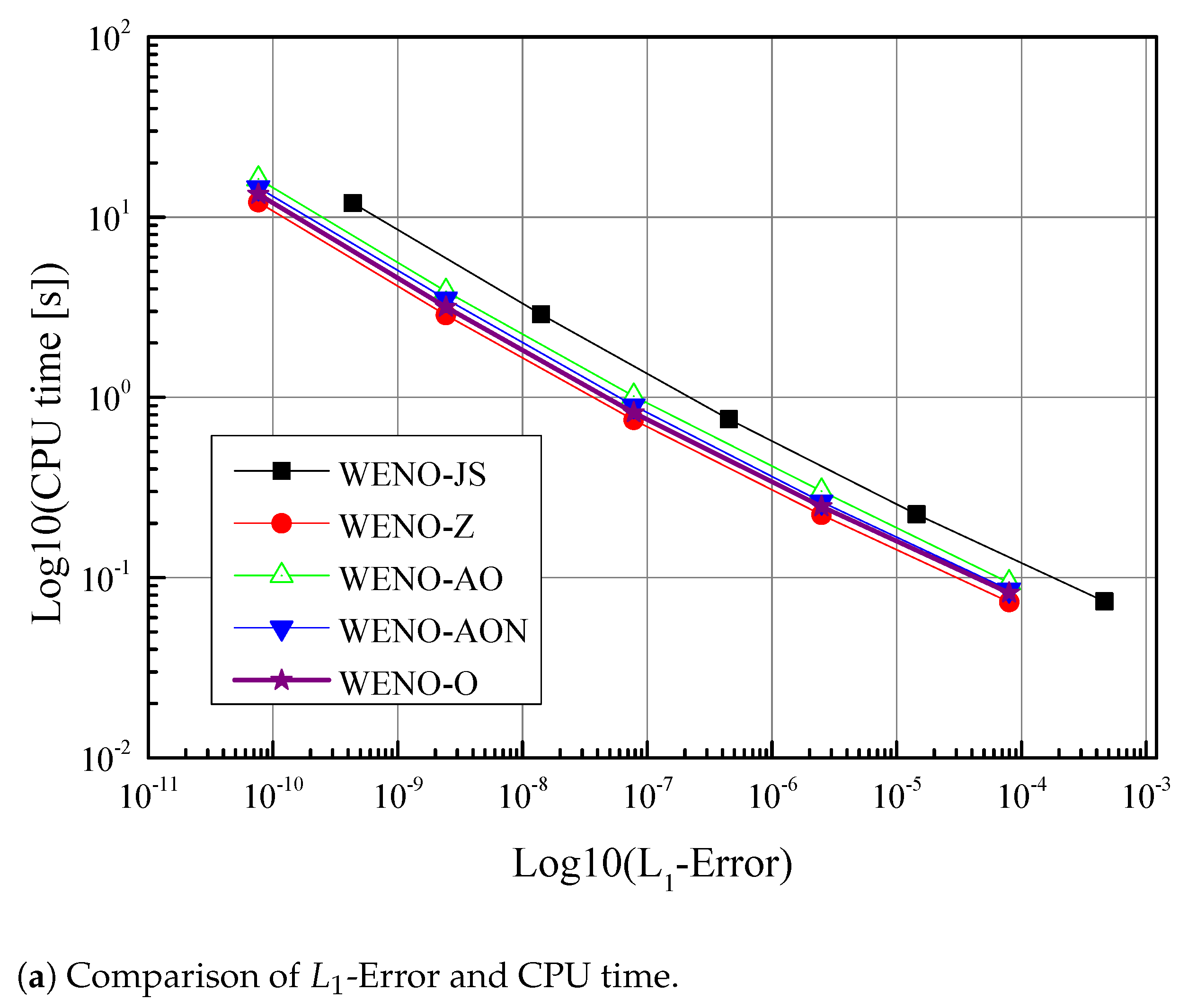
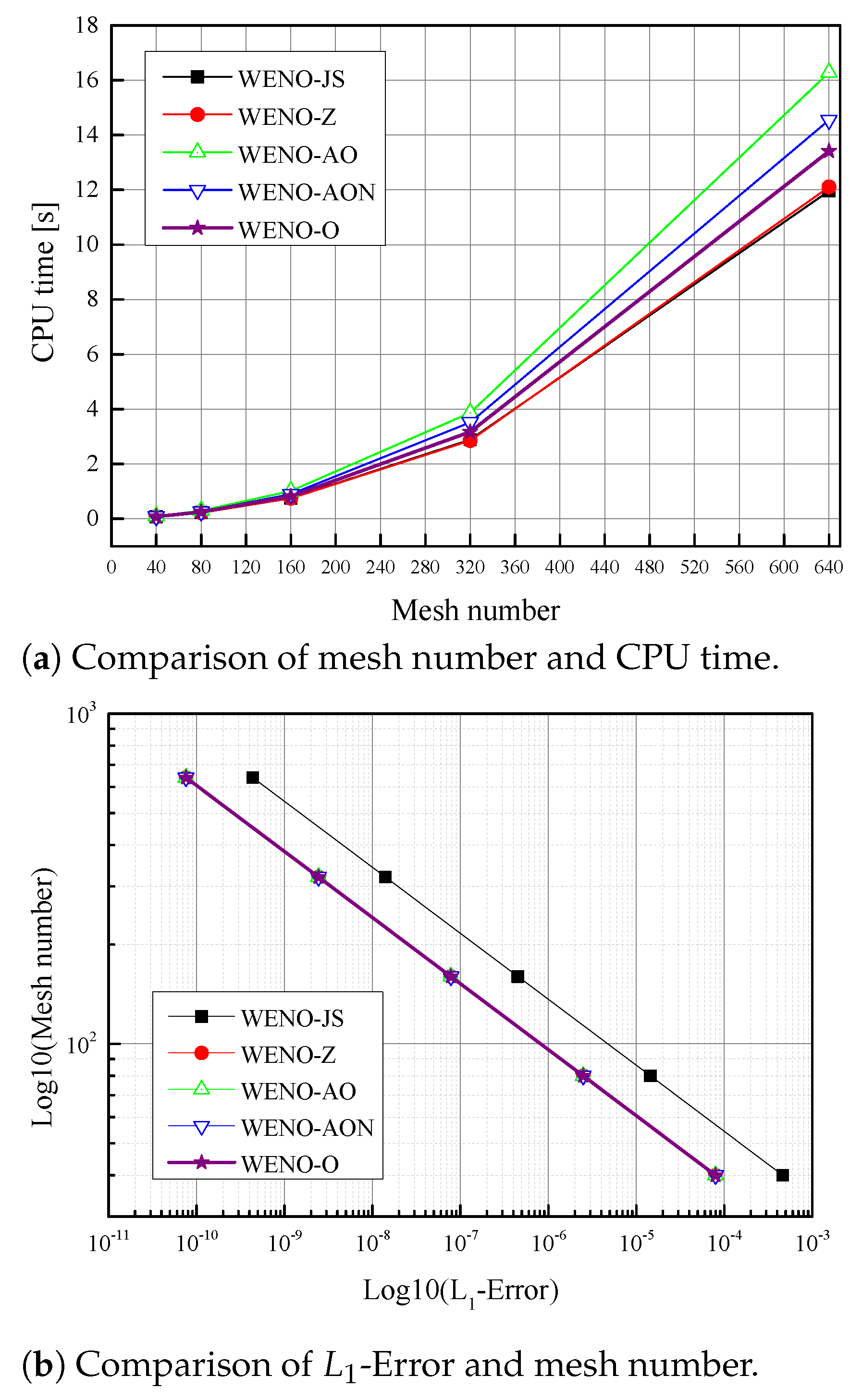
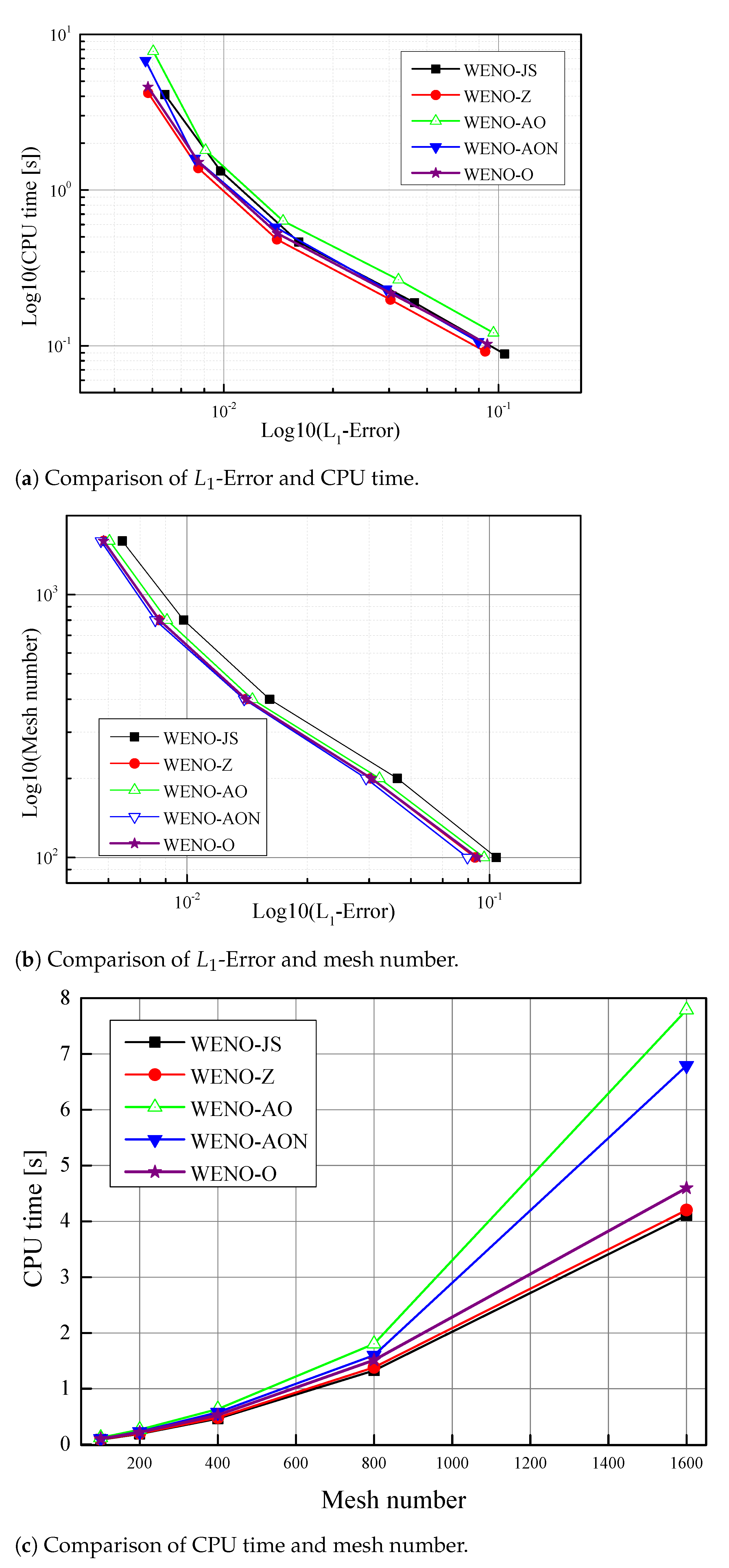
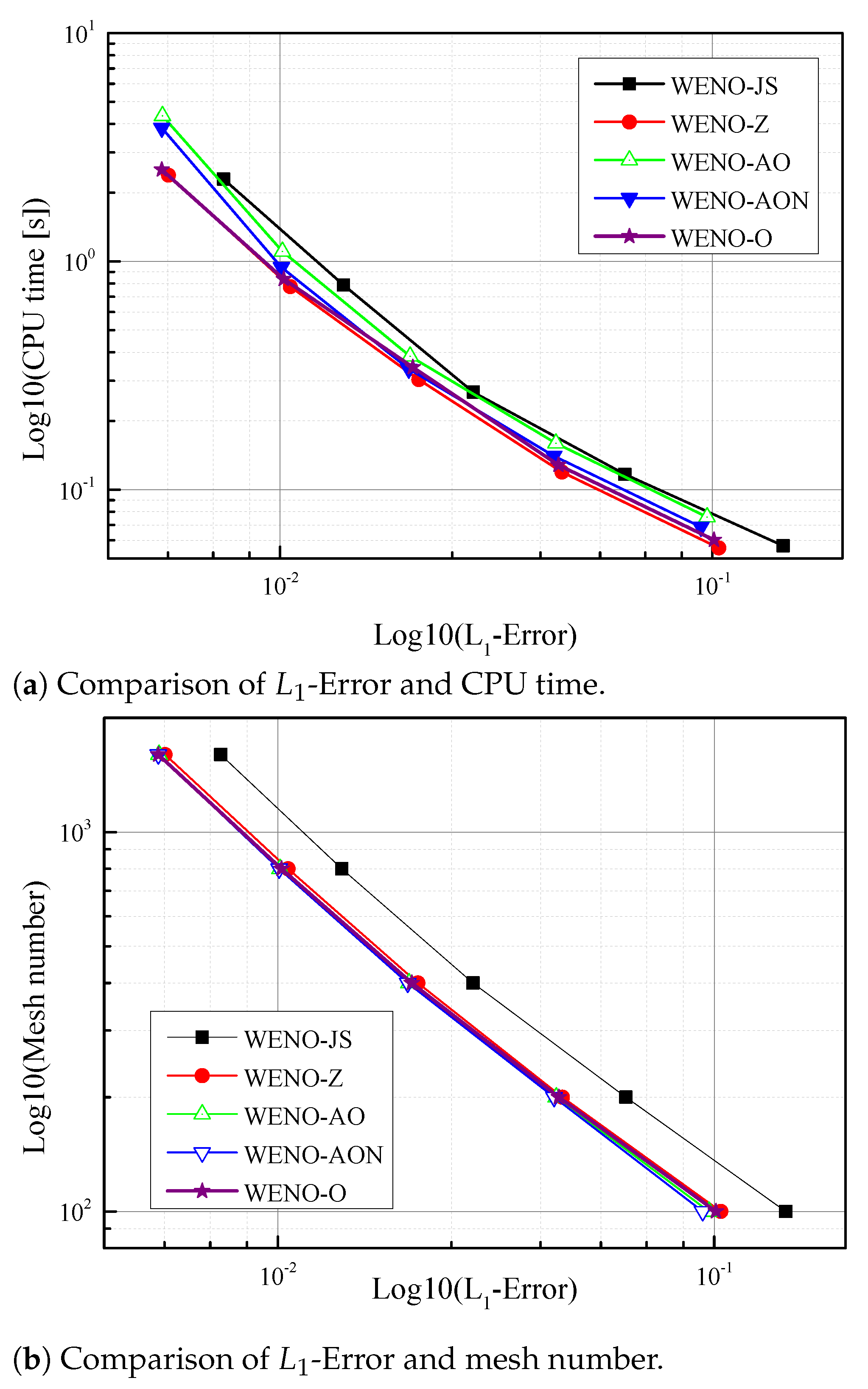
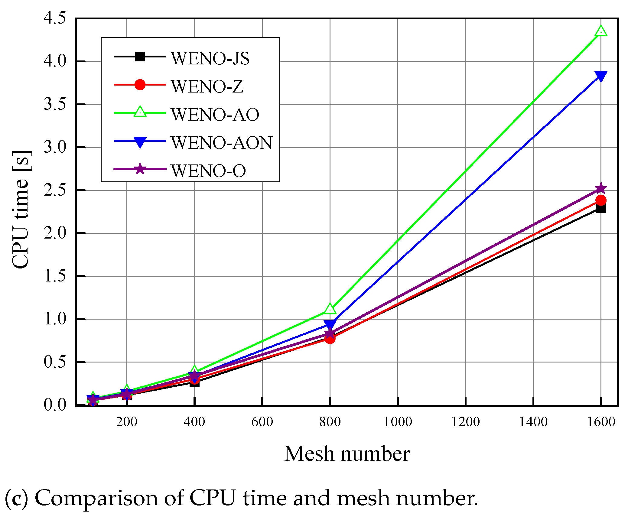
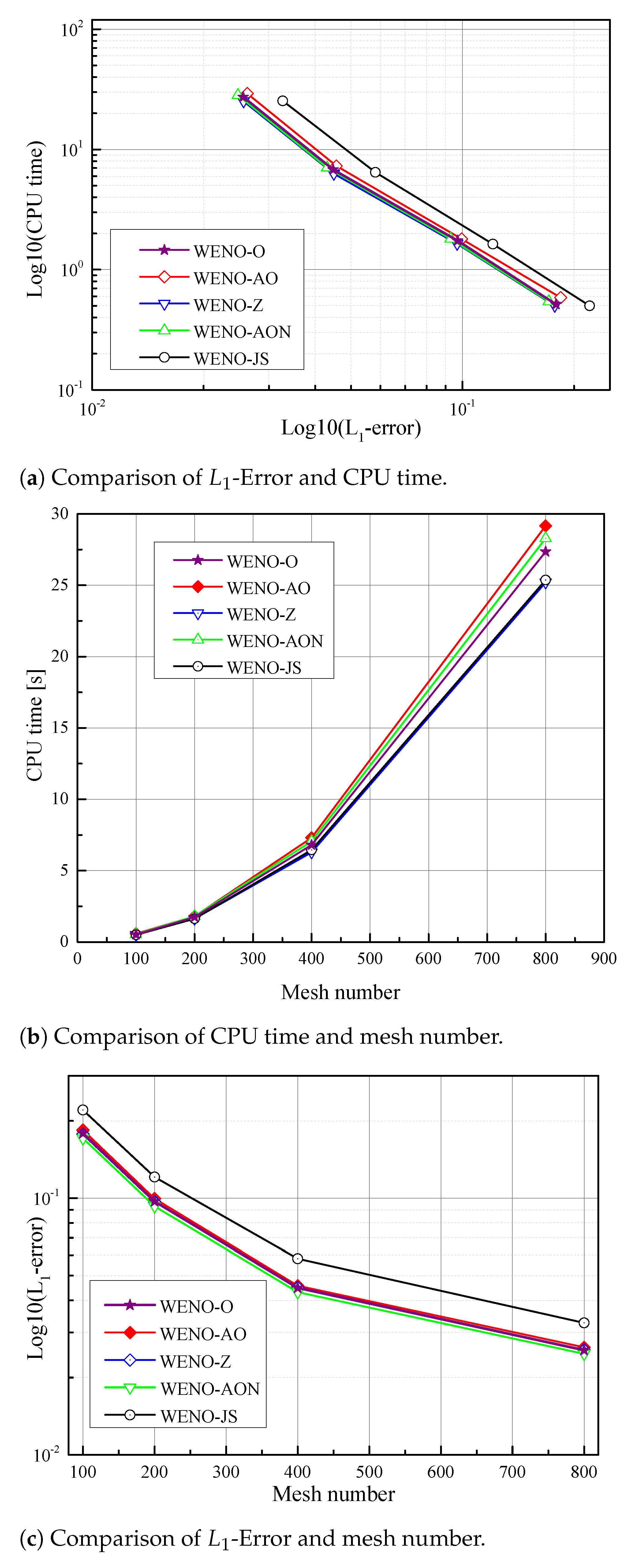
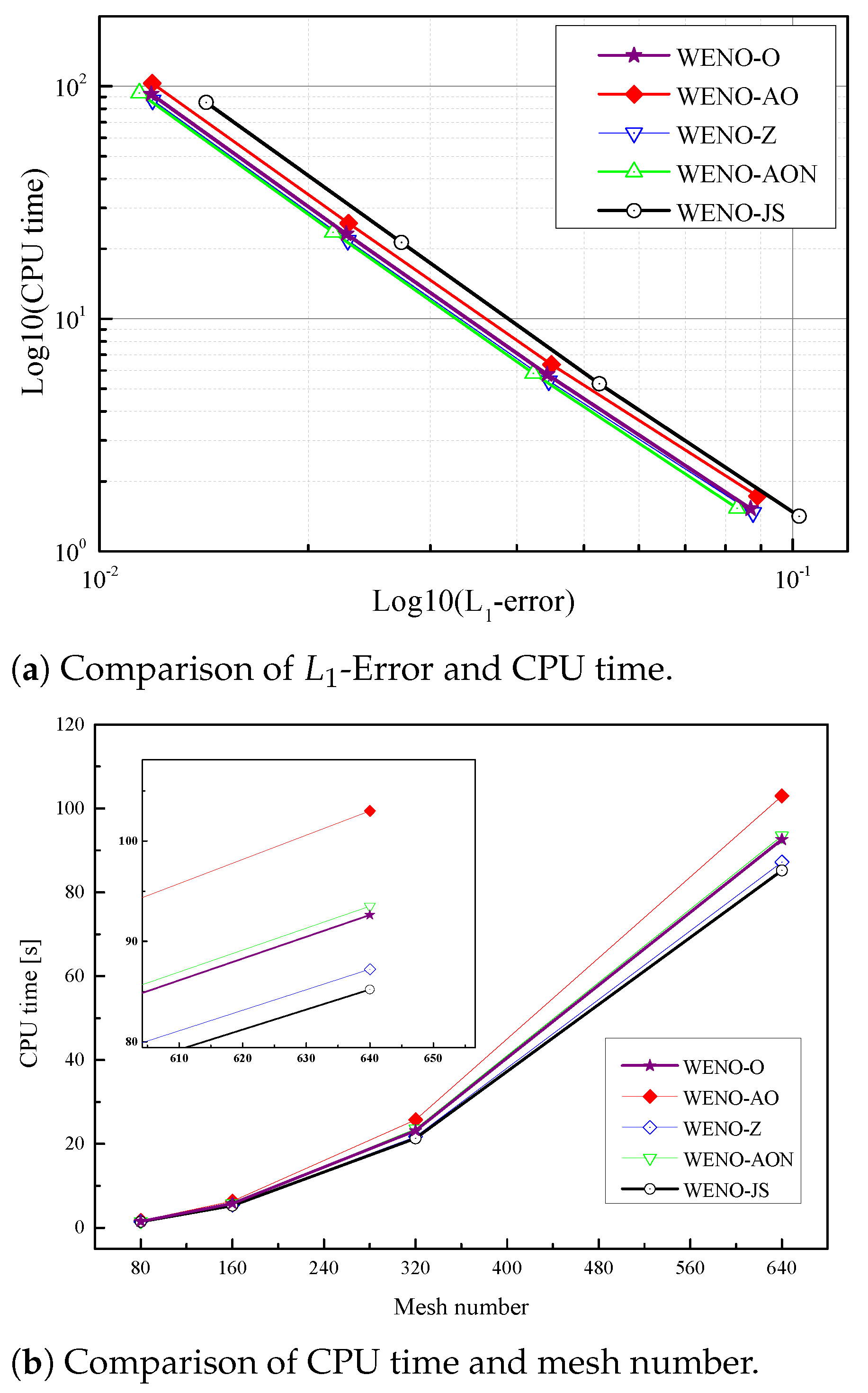
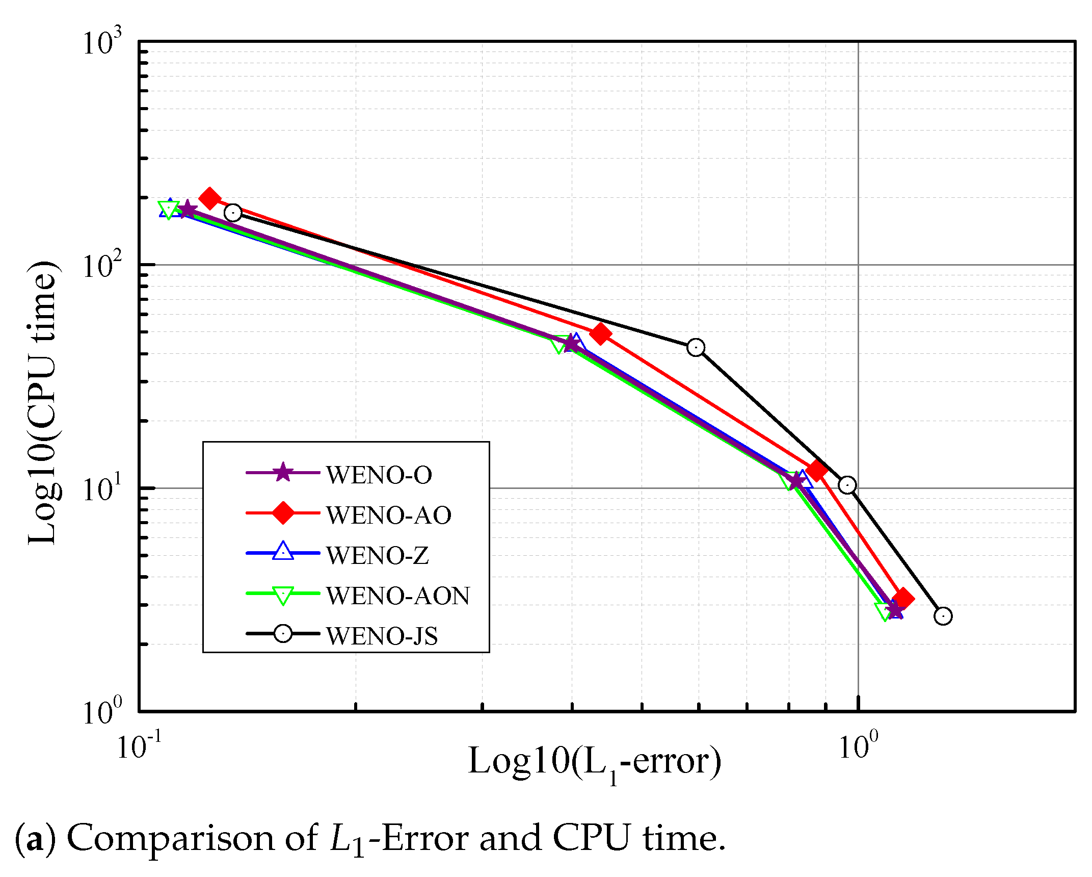
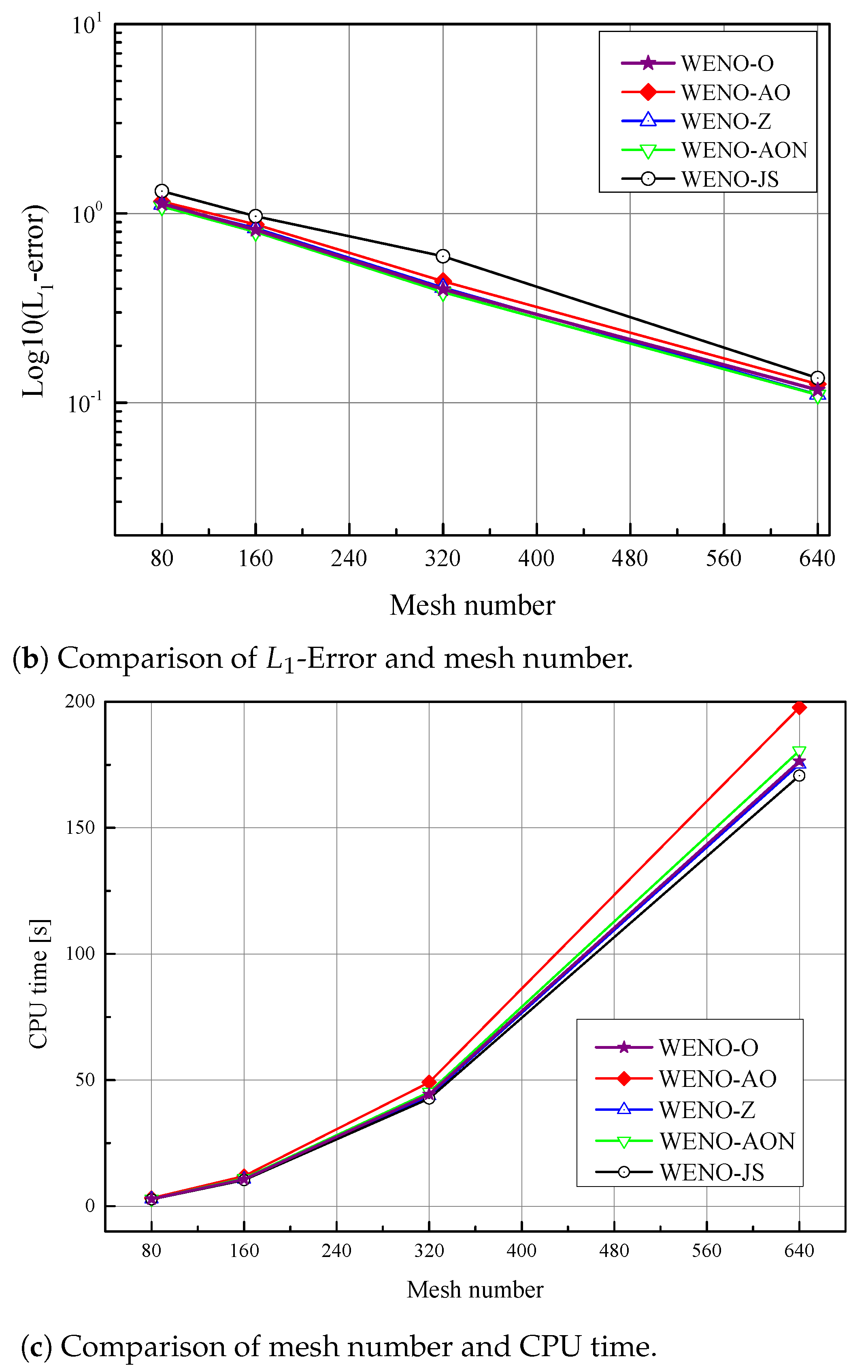
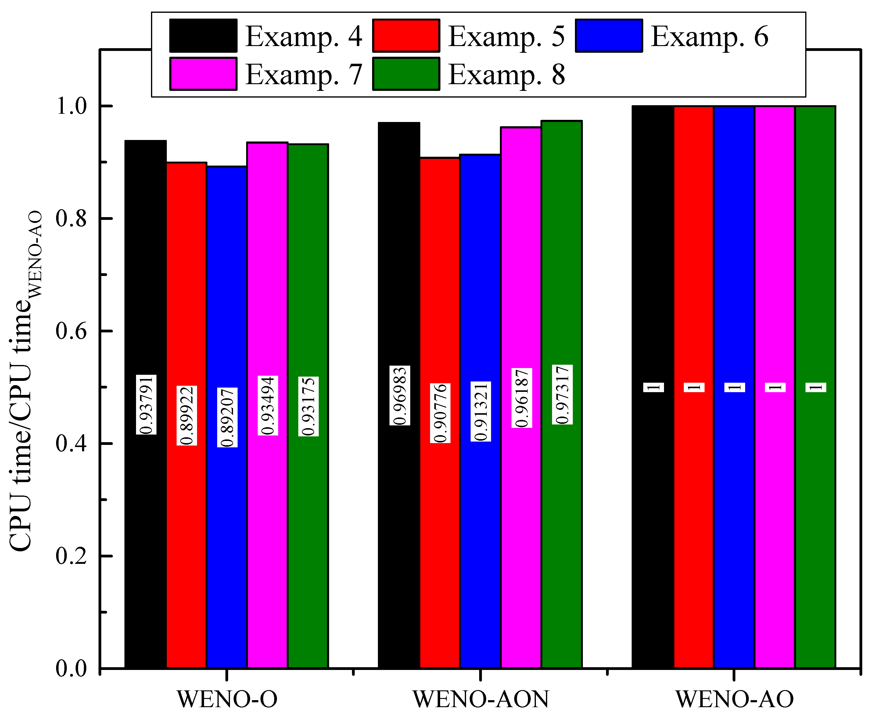
6.4. CPU Time Comparison

As shown in Section 3 (Table 1 and Table 2), the devised WENO-O scheme has decreased the complexity of adaptive order schemes (WENO-AO and WENO-AON). In this section, a comparison of CPU time of the devised WEON-O scheme and adaptive order schemes (WENO-AO and WENO-AON) is presented for six test cases (see Figure 22). In this figure, the CPU time of original WENO-AO scheme is used as a reference to other schemes (WENO-O and WENO-AON) because both schemes are modified version of WENO-AO scheme. The first modification of original WENO-AO scheme, WENO-AON scheme, showed less CPU time for all six test cases compared to WENO-AO scheme. The devised WENO-O scheme illustrated less CPU time than both original WENO-AO and WENO-AON schemes. One can conclude that the devised WENO-O scheme has decreased the computational cost of both WENO-AO and WENO-AON schemes.

7. Conclusions

It was shown that in previously published literature, adaptive order weighted essentially non- oscillatory WENO-AO(5,3) has increased the computational cost and complexity by introducing a complicated smoothness indicator for fifth-order linear reconstruction. Therefore, in this work we have proposed a simple smoothness indicator for fifth-order linear reconstruction. The devised smoothness indicator linearly combines the existing smoothness indicators of third-order linear reconstructions which reduces the complexity of that of WENO-AO(5,3) scheme. Then, the adaptive order weighted essentially non- oscillatory scheme uses the devised smoothness indicator is known as WENO-O scheme. We have demonstrated through eight numerical experiments that the WENO-O scheme has decreased the complexity and computational cost of adaptive order schemes (WENO-AO(5,3) and WENO-AON).

References

1. Harten, A.; Engquist, B.; Osher, S.; Chakravarthy, S.R. Uniformly high order accurate essentially non-oscillatory schemes, III. J. Comput. Phys. 1987, 71, 231–303. [Google Scholar] [CrossRef]
2. Shu, C.W.; Osher, S. Efficient implementation of essentially non-oscillatory shock-capturing schemes. J. Comput. Phys. 1988, 77, 439–471. [Google Scholar] [CrossRef] [Green Version]
3. Liu, X.D.; Osher, S.; Chan, T. Weighted essentially non-oscillatory schemes. J. Comput. Phys. 1994, 115, 200–212. [Google Scholar] [CrossRef] [Green Version]
4. Jiang, G.S.; Shu, C.W. Efficient implementation of weighted ENO schemes. J. Comput. Phys. 1996, 126, 202–228. [Google Scholar] [CrossRef] [Green Version]
5. Henrick, A.K.; Aslam, T.D.; Powers, J.M. Mapped weighted essentially non-oscillatory schemes: Achieving optimal order near critical points. J. Comput. Phys. 2005, 207, 542–567. [Google Scholar] [CrossRef]
6. Borges, R.; Carmona, M.; Costa, B.; Don, W.S. An improved weighted essentially non-oscillatory scheme for hyperbolic conservation laws. J. Comput. Phys. 2008, 227, 3191–3211. [Google Scholar] [CrossRef]
7. Musa, O.; Huang, G.; Yu, Z.; Li, Q. An improved Roe solver for high order reconstruction schemes. Comput. Fluids 2020, 207, 104591. [Google Scholar] [CrossRef]
8. Zhu, J.; Qiu, J. A new fifth order finite difference WENO scheme for solving hyperbolic conservation laws. J. Comput. Phys. 2016, 318, 110–121. [Google Scholar] [CrossRef]
9. Balsara, D.S.; Garain, S.; Shu, C.W. An efficient class of WENO schemes with adaptive order. J. Comput. Phys. 2016, 326, 780–804. [Google Scholar] [CrossRef] [Green Version]
10. Jung, C.Y.; Nguyen, T.B. A new adaptive weighted essentially non-oscillatory WENO-θ scheme for hyperbolic conservation laws. J. Comput. Appl. Math. 2018, 328, 314–339. [Google Scholar] [CrossRef]
11. Guo, J.; Jung, J.H. A RBF-WENO finite volume method for hyperbolic conservation laws with the monotone polynomial interpolation method. Appl. Numer. Math. 2017, 112, 27–50. [Google Scholar] [CrossRef]
12. Fan, P. High order weighted essentially nonoscillatory WENO-η schemes for hyperbolic conservation laws. J. Comput. Phys. 2014, 269, 355–385. [Google Scholar] [CrossRef] [Green Version]
13. Levy, D.; Puppo, G.; Russo, G. A third order central WENO scheme for 2D conservation laws. Appl. Numer. Math. 2000, 33, 415–422. [Google Scholar] [CrossRef]
14. Yamaleev, N.K.; Carpenter, M.H. A systematic methodology for constructing high-order energy stable WENO schemes. J. Comput. Phys. 2009, 228, 4248–4272. [Google Scholar] [CrossRef] [Green Version]
15. Guo, W.; Lin, G.; Christlieb, A.J.; Qiu, J. An adaptive WENO collocation method for differential equations with random coefficients. Mathematics 2016, 4, 29. [Google Scholar] [CrossRef] [Green Version]
16. Sheng, C.; Zhao, Q.; Zhong, D.; Ge, N. A Strategy to Implement High-Order WENO Schemes on Unstructured Grids. In Proceedings of the AIAA Aviation 2019 Forum, Dallas, TX, USA, 17–21 June 2019. [Google Scholar] [CrossRef]
17. Dong, H.; Lu, C.; Yang, H. The Finite Volume WENO with Lax–Wendroff Scheme for Nonlinear System of Euler Equations. Mathematics 2018, 6, 211. [Google Scholar] [CrossRef] [Green Version]
18. Peng, J.; Shen, Y. A novel weighting switch function for uniformly high-order hybrid shock-capturing schemes. Int. J. Numer. Methods Fluids 2017, 83, 681–703. [Google Scholar] [CrossRef] [Green Version]
19. Rathan, S. An improved non-linear weights for seventh-order weighted essentially non-oscillatory scheme. Comput. Fluids 2017, 156, 496–514. [Google Scholar] [CrossRef]
20. Wu, X.; Liang, J.; Zhao, Y. A new smoothness indicator for third-order WENO scheme. Int. J. Numer. Methods Fluids 2016, 81, 451–459. [Google Scholar] [CrossRef]
21. Xu, W.; Wu, W. Improvement of third-order WENO-Z scheme at critical points. Comput. Math. Appl. 2018, 75, 3431–3452. [Google Scholar] [CrossRef]
22. Zhao, Z.; Zhu, J.; Chen, Y.; Qiu, J. A new hybrid WENO scheme for hyperbolic conservation laws. Comput. Fluids 2019, 179, 422–436. [Google Scholar] [CrossRef]
23. Huang, C. WENO scheme with new smoothness indicator for Hamilton—Jacobi equation. Appl. Math. Comput. 2016, 290, 21–32. [Google Scholar] [CrossRef]
24. Huang, C.; Chen, L.L. A simple smoothness indicator for the WENO scheme with adaptive order. J. Comput. Phys. 2018, 352, 498–515. [Google Scholar] [CrossRef]
25. Kumar, R.; Chandrashekar, P. Simple smoothness indicator and multi-level adaptive order WENO scheme for hyperbolic conservation laws. J. Comput. Phys. 2018, 375, 1059–1090. [Google Scholar] [CrossRef] [Green Version]
26. Gottlieb, S.; Shu, C.W. Total variation diminishing Runge-Kutta schemes. Math. Comput. Am. Math. Soc. 1998, 67, 73–85. [Google Scholar] [CrossRef] [Green Version]
27. Lax, P.D. Weak solutions of nonlinear hyperbolic equations and their numerical computation. Commun. Pure Appl. Math. 1954, 7, 159–193. [Google Scholar] [CrossRef]
28. Sod, G.A. A survey of several finite difference methods for systems of nonlinear hyperbolic conservation laws. J. Comput. Phys. 1978, 27, 1–31. [Google Scholar] [CrossRef] [Green Version]
29. Shu, C.W.; Osher, S. Efficient implementation of essentially non-oscillatory shock-capturing schemes, II. J. Comput. Phys. 1989, 83, 32–78. [Google Scholar] [CrossRef]
30. Woodward, P.; Colella, P. The numerical simulation of two-dimensional fluid flow with strong shocks. J. Comput. Phys. 1984, 54, 115–173. [Google Scholar] [CrossRef]
31. Lax, P.D.; Liu, X.D. Solution of two-dimensional Riemann problems of gas dynamics by positive schemes. SIAM J. Sci. Comput. 1998, 19, 319–340. [Google Scholar] [CrossRef] [Green Version]
Figure 1. Schematic of the 1-D spatial discretization; 5-points stencil S 5 composed of three 3-points stencils S 0 , S 1 , S 2 .
Mathematics 09 00069 g001
Figure 2. The accuracy comparison of WENO-O with WENO-AO, WENO-AON, WENO-Z, and WENO-JS schemes for Example 1 (Section 6.1.1) on uniform mesh at t = 10 and C F L = ( Δ x ) 2 / 3 .
Mathematics 09 00069 g002aMathematics 09 00069 g002b
Figure 3. The performance comparison of WENO-O with WENO-AO, WENO-AON, WENO-Z, and WENO-JS schemes for Example 1 (Section 6.1.1) on different number of mesh points at t = 10 and C F L = ( Δ x ) 2 / 3 .
Mathematics 09 00069 g003
Figure 4. The accuracy comparison of WENO-O with WENO-AO, WENO-AON, WENO-Z, and WENO-JS schemes for Example 2 (Section 6.1.2) on uniform mesh at t = 1 and C F L = 0.1 .
Mathematics 09 00069 g004
Figure 5. Numerical solutions of Example 2 (Section 6.1.2) on uniform mesh with 200 cells at t = 1 and C F L = 0.1 .
Mathematics 09 00069 g005
Figure 6. Comparison of smoothness indicators β ¯ h , β h , and β ^ h of WENO-O, WENO-AO, and WENO-AON schemes, respectively, of Example 2 (Section 6.1.2).
Mathematics 09 00069 g006
Figure 7. The accuracy comparison of WENO-O with WENO-AO, WENO-AON, WENO-Z, and WENO-JS schemes for Example 3 (Section 6.1.3) on 1600 cells at t = 10 and C F L = 0.1 .
Mathematics 09 00069 g007aMathematics 09 00069 g007b
Figure 8. Numerical solutions of Example 3 (Section 6.1.3) on 1600 cells at t = 10 and C F L = 0.1 .
Mathematics 09 00069 g008
Figure 9. Zoomed regions of numerical solutions of Example 3 (Figure 8) (Section 6.1.3) on 1600 cells at t = 10 and C F L = 0.1 .
Mathematics 09 00069 g009aMathematics 09 00069 g009b
Figure 10. Comparison of smoothness indicators β ¯ h , β h , and β ^ h of WENO-O, WENO-AO, and WENO-AON schemes, respectively, of Example 3 (Section 6.1.3).
Mathematics 09 00069 g010
Figure 11. The accuracy comparison of the considered WENO schemes for Lax’s problem of Example 4 (Section 6.2.1) for density field at time t = 1.3 , C F L = 0.95 .
Mathematics 09 00069 g011
Figure 12. Numerical results of Lax’s problem of Example 4 (Section 6.2.1) for density field at time t = 1.3 , C F L = 0.95 with 200 cells for the considered WENO schemes.
Mathematics 09 00069 g012
Figure 13. Zoomed regions of numerical results of Lax’s problem of Example 4 (Figure 12) (Section 6.2.1) for density field at time t = 1.3 , C F L = 0.95 with 200 cells for the considered WENO schemes.
Mathematics 09 00069 g013aMathematics 09 00069 g013b
Figure 14. The accuracy comparison of considered WENO schemes for Sod’s problem of Example 5 (Section 6.2.2) for density field at time t = 2 , C F L = 0.1 .
Mathematics 09 00069 g014
Figure 15. Numerical results of Sod’s problem of Example 5 (Section 6.2.2) for density field at time t = 2 , C F L = 0.1 with 320 cells for the considered WENO schemes.
Mathematics 09 00069 g015
Figure 16. Zoomed regions of numerical results of Sod’s problem of Example 5 (Figure 15) (Section 6.2.2) for density field at time t = 2 , C F L = 0.1 with 320 cells for the considered WENO schemes.
Mathematics 09 00069 g016aMathematics 09 00069 g016b
Figure 17. The accuracy comparison of considered WENO schemes for Shu–Osher problem of Example 6 (Section 6.2.3) for density field at time t = 1.8 , C F L = 0.1 with 320 cells.
Mathematics 09 00069 g017aMathematics 09 00069 g017b
Figure 18. Numerical results of Shu–Osher problem of Example 6 (Section 6.2.3) for density field at time t = 1.8 , C F L = 0.1 with 320 cells for considered WENO schemes.
Mathematics 09 00069 g018
Figure 19. Equally spaced contours of two-dimensional double-Mach reflection of strong shock of Example 7 (Section 6.3.1) at time of 0.2 , C F L = 0.475 , [ 0 , 4 ] × [ 0 , 1 ] 1600 × 400.
Mathematics 09 00069 g019
Figure 20. Close view of equally spaced contours of two-dimensional double-Mach reflection of strong shock of Example 7 (Section 6.3.1) at time of 0.2, C F L = 0.475 , [ 0 , 4 ] × [ 0 , 1 ] 2-D domain and 1600 × 400 mesh size.
Mathematics 09 00069 g020aMathematics 09 00069 g020b
Figure 21. Equally spaced contours of two-dimensional Riemann problem of Example 8 (Section 6.3.2) at time 0.23, CFL = 0.6, [ 0 , 1 ] × [ 0 , 1 ] 2-D domain and 800 × 800 mesh size.
Mathematics 09 00069 g021
Figure 22. Comparison of CPU time of the adaptive order schemes (WENO-AO and WENO-AON) and proposed WENO-O scheme for six test cases.
Mathematics 09 00069 g022