Article

Fast Two-Stage Computation of an Index Policy for Multi-Armed Bandits with Setup Delays

Department of Statistics, Carlos III University of Madrid, 28903 Getafe, Spain
Mathematics 2021, 9(1), 52; https://doi.org/10.3390/math9010052
Submission received: 7 December 2020 / Revised: 23 December 2020 / Accepted: 24 December 2020 / Published: 29 December 2020
(This article belongs to the Special Issue Stochastic Models with Applications)

Abstract

:
We consider the multi-armed bandit problem with penalties for switching that include setup delays and costs, extending the former results of the author for the special case with no switching delays. A priority index for projects with setup delays that characterizes, in part, optimal policies was introduced by Asawa and Teneketzis in 1996, yet without giving a means of computing it. We present a fast two-stage index computing method, which computes the continuation index (which applies when the project has been set up) in a first stage and certain extra quantities with cubic (arithmetic-operation) complexity in the number of project states and then computes the switching index (which applies when the project is not set up), in a second stage, with quadratic complexity. The approach is based on new methodological advances on restless bandit indexation, which are introduced and deployed herein, being motivated by the limitations of previous results, exploiting the fact that the aforementioned index is the Whittle index of the project in its restless reformulation. A numerical study demonstrates substantial runtime speed-ups of the new two-stage index algorithm versus a general one-stage Whittle index algorithm. The study further gives evidence that, in a multi-project setting, the index policy is consistently nearly optimal.

1. Introduction

1.1. Background

In a much-studied version of the multi-armed bandit problem (MABP), a decision-maker selects one project to engage from a finite set of dynamic and stochastic projects at each of an infinite sequence of discrete-time periods. Each project is modeled as a classic (non-restless) bandit, so the engaged (active) project gives rewards and its state changes in a Markovian fashion, while rested (passive) projects neither produce rewards nor change state. The goal is to find a policy that selects one project to be engaged at each time, for maximizing the expected total geometrically discounted reward. The MABP is widely applicable, being regarded as a modeling paradigm of the exploration versus exploitation trade-off, and it has generated a vast literature (see the monograph [1] and the cited references there). Although the curse of dimensionality hinders direct numerical solution of its dynamic programming (DP) optimality equations for realistic-size models, as the size of the multi-dimensional state space grows exponentially with the number of projects, the MABP is solved optimally by a remarkably simple type of policy, a so-called (priority-) index policy. Index policies are based on defining for each project m an index λ m ( i m ) —a scalar mapping of the project state i m that depends only on the project parameters—and engage at each time a project of largest index. See, e.g., [2,3,4,5,6]. The index that is considered in [2], which is known in the literature as the Gittins index, extends to general Markovian bandits that which was introduced by Bellman in [7] for solving a Bernoulli bandit model.
However, appropriate modeling of potential applications often entails the incorporation of features that violate assumptions of the classic MABP. Regarding the assumption that passive projects do not give rewards, this is noncritical, since passive rewards can be readily eliminated through a linear transformation, as shown in [8]. Yet, other assumptions turn out to be critical, as index policies are typically suboptimal when they are violated. Such is the case, as demonstrated in [9], with the requirement that switching from engaging one project to another be costless, which is hardly realistic in many, if not most, applications. As stated in (p. 1, [9]), “it is diffificult to imagine a relevant economic decision problem in which the decision-maker may costlessly move between alternatives”. This motivates the interest of investigating extensions of the MABP that incorporate costs and/or delays for switching projects, which we will refer to generically, as in [10], as the multi-armed bandit problem with switching penalties (MABPSP).
Despite its practical relevance, the MABPSP has received relatively scant research attention when compared to the standard MABP. We refer the reader to [11] for a review of research on the MABPSP until the early 2000s. Important references on such early work include [9,10,12,13,14]. Additionally, see the survey [15]. Yet, the last decade has witnessed growing interest on variants of the MABPSP, being motivated by the relevance of switching penalties in a variety of application areas, including hiring and retention of workers who learn over time [16], online marketing [17,18], experiential learning [19], opportunistic channel access in communication networks [20,21], and continuation and abandonment decisions for research projects [22]. For recent theoretical work on properties of the MABPSP, see [23].
While the aforementioned work concerns discrete-state projects, ref. [24,25] address Markovian continuous-state projects with constant setup penalties (costs or delays).

1.2. Index Policies, Histeresis, and the Asawa and Teneketzis Index for the MABPSP

While switching penalties can generally be sequence-dependent, this paper will focus on the case that such penalties are separately defined for each project, while allowing them to depend on the project state. Specifically, we will assume that switching from engaging one project to another entails, similarly as in [26], a setdown cost to switch off the currently engaged project, and then a setup cost followed by a random setup delay to switch on the project about to be engaged. Note that setup delays can be used to model, e.g., time for preparing the ground or building infrastructure, as well as training or learning delays.
Although index policies are generally suboptimal for the MABPSP (see [9]), their ease of implementation motivates the interest of designing policies from such a class that perform well. An index policy in such a setting attaches to each project m an index λ m ( a m , i m ) , which now depends on both the previous action a m { 0 , 1 } (passive: 0 or active: 1) and the current project state i m . Thus, such an index decouples into a continuation index λ m ( 1 , i m ) , which applies when the project has already been set up, and a switching index λ m ( 0 , i m ) , to be used when the project has not yet been set up.
Drawing on intuition one would expect that switching penalties should discourage frequent switching and, hence, should cause a histeresis effect on the structure of optimal policies. Thus, it should be optimal to stick longer to the currently engaged project that would be the case in the absence of such penalties. As put in (p. 691 [9]), “it is obvious that in comparing two otherwise identical arms, one of which was used in the previous period, the one which was in use must necessarily be more attractive than the one which was idle”. To be consistent with such a hysteresis property, the indices of a project m must satisfy that
λ m ( 1 , i m ) λ m ( 0 , i m ) for   every   project   state   i m .
Note that index policies can be optimal in special cases of the MABPSP, as shown in [13], in a model for scheduling a multi-class batch of stochastic jobs.
An intuitively appealing choice of index, extending that in [13], is that considered by Asawa and Teneketzis in [10]—which we will refer to in the sequel as the AT index—for a project having either a constant (not dependent on the project state) setup cost or a constant setup delay distribution, and no setdown costs. It is shown in [10] that the AT index provides a partial characterization of optimal policies for the version of the MABPSP considered there. The continuation AT index of a project is simply its Gittins index. As for the switching AT index, it is the highest rate of discounted expected reward minus setup cost per unit of discounted expected active time (counting the setup delay as active time) that can be attained from an initially passive project by first setting it up and then engaging it for a random duration that is given by a stopping time.

1.3. Index Computation

Efficient index computation is a key issue that must be addressed in practice for deploying an index policy for the MABPSP. For a project with n states and constant setup cost, but without setup delays, (Section III.C [10]) shows that the 2 n AT continuation and switching index values λ * ( a , i ) can be computed as the Gittins index of an appropriately defined 2 n -state project with augmented state ( a , i ) . Because computing the Gittins index has, in general, a cubic operation complexity in the number of states, such an approach results in an eightfold increase in complexity relative to that of computing the continuation index only.
A faster two-stage approach for a project with both setup and setdown costs—but no setup delays—that can be state-dependent was given by the author in [27]. The proposed algorithm computes, in the first stage, the continuation index and certain extra quantities by applying the ( 4 / 3 ) n 3 + O ( n 2 ) fast-pivoting algorithm with extended output presented in [28]. Subsequently, in the second stage, it computes the switching index in at most O ( n 2 ) operations. Hence, computing with that algorithm the 2 n AT index values entails only a twofold complexity increase relative to the ( 2 / 3 ) n 3 + O ( n 2 ) operation count to compute the continuation (Gittins) index only through the fast-pivoting algorithm (without extended output) given in [28]. Further, ref. [27] reports on the results of a numerical study demonstrating that the resulting index policy for the version of the MABPSP considered there is close to optimal and outperforms the Gittins index policy by a wide margin, across a wide range of instances.

1.4. Approach via Restless Bandit Reformulation, Whittle Index, and Indexability

The two-stage index algorithm shown in [27] exploits the reformulation of a project with switching costs and states i as a restless bandit—i.e., a project that can change state while passive—without such costs, moving across augmented states ( a , i ) . In that way, the MABP with switching costs is cast as a multi-armed restless bandit problem (MARBP) without them, which allows for the deployment of theoretical and algorithmic results on restless bandit indexation, as introduced in [29] by Whittle. Such a theory has been developed in [30,31,32,33] by the author. Additionally, see the survey [34].
Thus, while the MARBP is generally intractable, as it is known to be PSPACE-hard (see [35]), Whittle introduced, in [29], a widely applied heuristic index policy. For a sample of recent applications, see, for example [36,37,38,39,40,41,42,43,44,45,46,47,48]. Yet, the Whittle index is only defined for a limited class of restless bandits, called indexable, and it is nontrivial to verify whether such an indexability property holds for a given model. The work of the author referred to above provides sufficient indexability conditions for general restless bandits, which are grounded on satisfaction by project performance metrics of partial conservation laws (PCLs), together with an adaptive-greedy index algorithm that computes the Whittle index (and extensions thereof) under such conditions.
Such a PCL-indexability approach is deployed in [27], using the result that the AT index of a non-restless bandit with switching costs (but no switching delays) is its Whittle index in the project’s restless reformulation. The corresponding restless bandit model is shown to satisfy the PCL-indexability conditions, ensuring that its Whittle index can be computed by the adaptive-greedy algorithm. Special structure and the results in [49] are then used in [27] in order to decouple that algorithm into a faster two-stage method.

1.5. Motivation and Goals

Yet, no method is given in Asawa and Teneketzis [10] in order to compute their proposed index under switching delays. The latter’s relevance in applications, along with the tractability and effectiveness of the AT index policy in the pure-switching-costs case, motivates the interest to extend the restless bandit indexation approach for developing an efficient index algorithm for bandits that incorporate both switching costs and delays, which is the first goal of this paper.
Carrying out such an extension turns out to raise methodological research challenges on restless bandit indexation. Thus, when a Markovian non-restless bandit with switching delays is reformulated as a semi-Markov restless bandit without them, it is found that the resultant model need not satisfy the PCL-indexability conditions that were the cornerstone to the analyses presented in Niño-Mora [27] for the pure-switching-costs case. This motivates us to significantly extend the scope of previous theory, obtaining more powerful sufficient indexability conditions, which are both easier to apply and applicable to a wider class of models, including that of concern herein. That is the second goal of this paper. The third goal entails assessing the runtime performance of the proposed index algorithm, and evaluating the performance of the resulting index policy, both in terms of its optimality gap and its improvement over alternative simpler index policies.

1.6. Contributions

Concerning the second goal, on general restless bandit methodology, we introduce, for finite-state restless bandits, significantly simpler and less stringent sufficient conditions for indexability than the former PCL-based conditions, under which it is also assured that the adaptive-greedy algorithm computes the MPI. We further show such conditions to be necessary, in that any indexable finite-state restless bandit satisfies them. Thus, the new conditions furnish a complete characterization of indexability, which can be used in order to analytically establish a priori that a restless bandit model of concern is indexable—as opposed to numerically verifying a posteriori that a given instance is indexable.
As for the first goal, we deploy the new indexability conditions in the restless bandit reformulation of a non-restless bandit with switching delays and costs. Because the AT index emerges as the Whittle index in such a reformulation, we are thus assured that the adaptive-greedy algorithm will compute it. The complexity of such an algorithm is then reduced by exploiting special structure, which again yields a substantially faster two-stage method. In the first stage, the continuation index is computed in ( 4 / 3 ) n 3 + O ( n 2 ) arithmetic operations, and then the switching index is computed in the second stage in only—at most— ( 5 / 2 ) n 2 + O ( n ) operations. Thus, we obtain a two-stage algorithm that computes both the continuation and switching index in roughly twice the time that is required to compute the continuation index alone (if the latter were computed using the fast-pivoting ( 2 / 3 ) n 3 + O ( n 2 ) algorithm in [34]).
Regarding the third goal, we report on a computational study demonstrating the substantial runtime speed-up that is achieved by the two-stage algorithm relative to direct application of the one-stage adaptive-greedy algorithm. This study further reports on experiments providing evidence that the index policy is close to optimal and it attains significant gains against a benchmark index policy across a wide range of randomly generated instances with two and three projects.

1.7. Structure of the Paper and Notation

The rest of the paper proceeds as follows. Section 2 describes the MABPSP model of concern, reviews the AT index, and describes the restless bandit indexation approach to be applied. Section 3 lays the groundwork for such an approach in a general framework of finite-state restless bandits, introducing the new methological advances on restless bandit indexation. Section 4 deploys the new results in the special restless bandit model that arises from the reformulation of a non-restless bandit with switching penalties, which culminates in the development of the new two-stage index algorithm in Section 5. Section 6 presents some qualitative properties on how the index depends on setup and setdown penalties. Finally, Section 7 presents and discusses the numerical study.
Because the notation of the paper may be hard to follow, Table 1 summarizes it for the reader’s convenience.

2. MABPSP Model and Its Semi-Markov MARBP Reformulation

A decision-maker ponders how to prioritize the allocation of effort to M dynamic and stochastic projects that are labelled by m M { 1 , , M } , one of which must be engaged (active) at each of a sequence of decision periods t k Z + { 0 , 1 , 2 , } , with t 0 = 0 and t k as k , while others are rested (passive). Switching projects on and off entails setup and setdown delays and costs, respectively. A setup (resp. setdown) delay on a project is necessarily followed by a period in which the project is worked on (resp. rested), i.e., the times at which a setup or a setdown delay are completed are not decision periods. We will say that a project is “active” when it is either being engaged (worked upon) or undergoing a setup or a setdown delay. Let X m ( t ) and A m ( t ) denote the prevailing state, which belongs to the finite state space X m , and action for project m at time t ( A m ( t ) = 1 : active; A m ( t ) = 0 : passive), and let A m ( t ) A m ( t 1 ) denote the previously chosen action, with A m ( 0 ) indicating the initial setup status.
While project m is passive, it neither accrues rewards nor changes state. Switching it on when it lies in state i m entails a lump setup cost c m ( i m ) , followed by a random setup delay of duration ξ m ( i m ) periods, whose z-transform is ϕ m ( z ; i m ) E z ξ m ( i m ) , over which no rewards are earned. After such a setup, the project must be engaged, yielding a reward R m ( i m ) , after which its state moves at the next period to j m with transition probability p m ( i m , j m ) . After at least one period in which the project is engaged, it may be decided to switch it off. If this is done when the project lies in state j m , then a lump setdown cost d m ( j m ) is incurred, followed by a random setdown delay of duration η m with z-transform ψ m ( z ) E z η m , over which no rewards accumulate. Subsequently, the project remains passive for one or more periods. Note that setup delay distributions are allowed to be state-dependent, whereas setdown delay’s are not (cf. Section 2.1). Rewards and costs are geometrically time-discounted with factor β < 1 . We write, in what follows, the above z-transforms evaluated at z = β simply as ϕ m ( i m ) and ψ m .
Actions are prescribed through a scheduling policy π , which is chosen from the class Π of policies that are admissible, i.e., nonanticipative with respect to the history of states and actions, and engaging one project at a time. The MABPSP (cf. Section 1) is concerned with finding an admissible scheduling policy that attains the maximum expected total discounted reward net of switching costs.
This problem can be cast into the framework of semi-Markov decision problems (SMDPs) by including into the state of each project m the last action taken, i.e., by using the augmented state Y m ( t ) ( A m ( t ) , X m ( t ) ) , which belongs to the augmented state space Y m { 0 , 1 } × X m . Thus, one obtains a multidimensional SMDP having joint state Y ( t ) ( Y m ( t ) ) m M and joint action A ( t ) ( A m ( t ) ) m M . This is a special type of semi-Markov MARBP (cf. Section 1), as the constituent projects become restless in such a reformulation.
Rewards and dynamics for the reformulated project m are as follows, where R m a m ( a m , i ) and p m a m ( ( a m , i m ) , ( b m , j m ) ) denote the one-stage (i.e., from t k to t k + 1 ) expected reward and transition probability, which results from taking action a m in state Y m ( t k ) = ( a m , i m ) . On the one hand, if, in period t k , the project lies in state ( 1 , i m ) and it is again engaged, it yields the reward R m 1 ( 1 , i m ) R m ( i m ) and its state transitions at t k + 1 = t k + 1 to ( 1 , j m ) with probability p m 1 ( ( 1 , i m ) , ( 1 , j m ) ) p m ( i m , j m ) . If, instead, the project is switched off, it gives the reward R m 0 ( 1 , i m ) d m ( i m ) and its state moves at t k + 1 = t k + η m + 1 to ( 0 , i m ) with probability 1, i.e., p m 0 ( ( 1 , i m ) , ( 0 , i m ) ) 1 . On the other hand, if the project occupies at time t k the state ( 0 , i m ) and is then switched on, it yields the expected reward
R m 1 ( 0 , i m ) E [ c m ( i m ) + β ξ m ( i m ) R m ( i m ) ] = c m ( i m ) + ϕ m ( i m ) R m ( i m )
until the following decision time t k + 1 = t k + ξ m ( i m ) + 1 , in which the project state transitions to ( 1 , j m ) with probability p m 1 ( ( 0 , i m ) , ( 1 , j m ) ) p m ( i m , j m ) . If the project is kept idle, then it gives no reward, i.e., R m 0 ( 0 , i m ) 0 , and its state remains frozen up to t k + 1 = t k + 1 , so p m 0 ( ( 0 , i m ) , ( 0 , i m ) ) 1 .
Thus, the MABPSP of concern is formulated as the semi-Markov MARBP
maximize π Π E Y ( 0 ) π k = 0 m = 1 M R m A m ( t k ) ( Y m ( t k ) ) β t k ,
where E Y ( 0 ) π [ · ] is expectation under policy π conditioned on starting from the joint state Y ( 0 ) .

2.1. Reduction to the Case with No Setdown Penalties

We next show that one can restrict attention with no loss of generality to the case that there are no setdown penalties, which will allow for us to simplify subsequent analyses. Imagine that, say, at time t = 0 , a passive project is set up and is then worked on for a random number of periods determined by a stopping time τ 1 , after which it is set down. Dropping the label m, denote, by R = ( R j ) j X , c = ( c j ) j X , and d = ( d j ) j X , the active reward vector, and the setup and setdown cost vectors. Denote, by ϕ = ( ϕ j ) j X , the setup delay z-transform vector and by ψ the constant setdown delay transform, both evaluated at z = β . The total discounted expected net reward that is obtained from the project over such a time interval, starting from the augmented state Y ( 0 ) = ( 0 , i ) , is
F ( 0 , i ) τ ( R , c , d , ϕ , ψ ) E ( 0 , i ) τ c i + β ξ i t = 0 τ 1 R X ( t ) β t d X ( τ ) β ξ i + τ ,
where ξ i is the setup delay. The corresponding discounted active time expended on the project is
G ( 0 , i ) τ ( ϕ , ψ ) E ( 0 , i ) τ 1 β ξ i 1 β + β ξ i t = 0 τ 1 β t + 1 β η 1 β β ξ i + τ ,
where, as pointed out above, the setup and setdown delays ξ i and η are both considered to be active time.
In the next result, which extends Lemma 3.4 of [27] to the present setting, I is the identity matrix indexed by X , P = ( p i j ) i , j X , 0 is a vector of zeros, and ϕ · d ( ϕ j d j ) j X .
Lemma 1.
(a)
F ( 0 , i ) τ ( R , c , d , ϕ , ψ ) = F ( 0 , i ) τ ( ψ 1 ( R + ( I β P ) d ) , c + ϕ · d , 0 , ψ ϕ , 1 ) .
(b)
G ( 0 , i ) τ ( ϕ , ψ ) = G ( 0 , i ) τ ( ψ ϕ , 1 ) .
Proof. 
(a) Use the identity
d X ( τ ) β τ = d i t = 0 τ 1 ( d X ( t ) β d X ( t + 1 ) ) β t
to write
F ( 0 , i ) τ ( R , c , d , ϕ , ψ ) E ( 0 , i ) τ c i + β ξ i t = 0 τ 1 R X ( t ) β t d Y ( τ ) β ξ i + τ = c i + ϕ i E ( 0 , i ) τ t = 0 τ 1 R X ( t ) β t d Y ( τ ) β τ = c i + ϕ i d i + E ( 0 , i ) τ t = 0 τ 1 ( R X ( t ) + d X ( t ) β d X ( t + 1 ) ) β t = c i ϕ i d i + ϕ i E ( 0 , i ) τ t = 0 τ 1 ( R X ( t ) + d X ( t ) β d X ( t + 1 ) ) β t = c i ϕ i d i + ϕ i ψ E ( 0 , i ) τ ψ 1 t = 0 τ 1 ( R X ( t ) + d X ( t ) β d X ( t + 1 ) ) β t = F ( 0 , i ) τ ( ψ 1 ( R + ( I β P ) d ) , c + ϕ · d , 0 , ψ ϕ , 1 ) .
(b) This part follows by writing
G ( 0 , i ) τ E ( 0 , i ) τ 1 β ξ i 1 β + β ξ i t = 0 τ 1 β t + 1 β η 1 β β ξ i + τ = 1 ϕ i 1 β + ϕ i E i τ t = 0 τ 1 β t + 1 ψ 1 β β τ = 1 ϕ i 1 β + ϕ i E ( 0 , i ) τ t = 0 τ 1 β t + 1 ψ 1 β 1 ( 1 β ) t = 0 τ 1 β t = 1 ϕ i ψ 1 β + ϕ i E ( 0 , i ) τ t = 0 τ 1 ( 1 ( 1 ψ ) ) β t = 1 ϕ i ψ 1 β + ϕ i ψ E ( 0 , i ) τ t = 0 τ 1 β t = G ( 0 , i ) τ ( ψ ϕ , 1 ) .
 □
Lemma 1 can be used in order to eliminate setdown penalties: it suffices to incorporate them into new setup costs, setup delay transforms, and active rewards, while using the transformations
c ˜ j c j + ϕ j d j , ϕ ˜ j ψ ϕ j , and R ˜ ψ 1 ( R + ( I β P ) d ) .
Note that such a reduction would not have been accomplished had the setdown delay transform not been constant. In the case c j c and d j d , we obtain c ˜ j c + d ϕ j and R ˜ j = ( R j + ( 1 β ) d ) / ψ .
Accordingly, we will focus henceforth on the normalized case without setdown penalties d j 0 , ψ 1 .

2.2. The AT Index

We next consider the AT index of a project with setup penalties—dropping again the label m—extending the original definitions in [10]. The continuation AT index is
λ ( 1 , i ) AT max τ 1 E i τ t = 0 τ 1 R X ( t ) β t E i τ t = 0 τ 1 β t ,
where τ 1 is a stopping time for engaging the project starting in state i when it is already set up; hence, λ ( 1 , i ) AT is just the project’s Gittins index. As for the switching AT index, it is given by
λ ( 0 , i ) AT max τ 1 c i + E i τ β ξ i t = 0 τ 1 R X ( t ) β t E i τ t = 0 ξ i 1 β t + β ξ i t = 0 τ 1 β t = max τ 1 c i + ϕ i E i τ t = 0 τ 1 R X ( t ) β t 1 ϕ i 1 β + ϕ i E i τ t = 0 τ 1 β t ,
where now τ is a stopping-time rule that is followed after the project has been set up in state i.
The following requirements will be assumed henceforth on setup costs and setup delay transforms, which extend the corresponding conditions in [10].
Assumption 1.
The following holds:
(i)
non-negative setup costs: c j 0 for j X .
(ii)
non-negative rewards: If some setup delay can be positive, i.e., ϕ 1 , then R j 0 for j X .
The next result shows that Assumption 1 ensures the satisfaction of the hysteresis property in (1).
Lemma 2.
Under Assumption 1, λ ( 1 , i ) AT λ ( 0 , i ) AT for i X .
Proof. 
For a given state i X and stopping-time rule τ as above, write G i τ E i τ [ t = 0 τ 1 β t ] and F i τ E i τ [ t = 0 τ 1 R X ( t ) β t ] . Now, Assumption 1 ensures that c i 0 and F i τ 0 , and hence
F i τ G i τ c i + ϕ i F i τ 1 ϕ i 1 β + ϕ i G i τ = 1 G i τ ( 1 β ) c i G i τ + ( 1 ϕ i ) F i τ 1 ϕ i + ( 1 β ) ϕ i G i τ 0 ,
Further, (9), (7), and (8) immediately yield that λ ( 1 , i ) AT λ ( 0 , i ) AT , which completes the proof. □

3. New Methodological Results on Restless Bandit Indexation

This section presents new results on restless bandit indexation, which, besides having an intrinsic interest, are required and form the basis for the approach to non-restless bandits with switching times that is deployed in later sections.

3.1. Indexable Restless Bandits and the Whittle Index

Consider a semi-Markov restless bandit, representing a dynamic and stochastic project whose state Y ( t ) transitions over time periods t = 0 , 1 , 2 , through the finite state space Y . The project’s evolution is governed by a policy π that is taken from the class Π of nonanticipative randomized policies, which, at each of an increasing sequence t k of decision periods with t 0 = 0 and t k as k , prescribes an action A ( t k ) { 0 , 1 } that determines the status during the ensuing stage until the next decision period t k + 1 (1: active; 0: passive). Taking action A ( t k ) = a at time t k when the project occupies state Y ( t k ) = y has the following consequences over the following stage, relative to a given one-period discount factor 0 < β < 1 : an expected total discounted amount of reward R y a and of a generic resource Q y a 0 is earned and expended, respectively; further, the joint distribution of the stage’s duration t k + 1 t k and its final state Y ( t k + 1 ) is given through the discounted transition transform ϕ y y a E β t k + 1 t k 1 { Y ( t k + 1 ) = y } | Y ( t k ) = y , A ( t k ) = a , where 1 { · } denotes an event indicator.
It will be convenient to partition Y into the (possibly empty) set of uncontrollable states
Y { 0 } i Y : Q y 0 = Q y 1 and ϕ y y 0 ϕ y y 1 , y Y ,
where both actions entail identical resource consumptions and dynamics, and the remaining set Y { 0 , 1 } Y \ Y { 0 } of controllable states, which is assumed to consist of N = | Y { 0 , 1 } | 1 elements. The notation Y { 0 } is meant to reflect the convention that the passive action a = 0 is chosen in uncontrollable states.
The value of the rewards earned and amount of resource expended by a policy π starting from state y is evaluated, respectively, by the discounted reward and resource consumption metrics
F y π E y π k = 0 R Y ( t k ) A ( t k ) β t k and G y π E y π k = 0 Q Y ( t k ) A ( t k ) β t k .
Let us introduce a parameter λ representing the resource unit price, and consider the λ-price problem
maximize π Π F y π λ G y π ,
which concerns finding a policy that maximizes the value of rewards earned minus the cost of resources expended. Because (10) is an infinite-horizon finite-state and -action SMDP, by standard results it is solved by stationary deterministic policies that are characterized by the solutions to the following DP equations, where V y * ( λ ) denotes the optimal value starting from y under price λ :
V y * ( λ ) = max a { 0 , 1 } R y a λ Q y a + y Y ϕ y y a V y * ( λ ) , y Y .
Such a project is said to be indexable (cf. [29]), if, for each controllable state y Y { 0 , 1 } , there exists a unique break-even price λ y * , such that: it is optimal to engage the project in state y if and only if λ λ y * , and it is optimal to rest it if and only if λ λ y * . Or, in terms of the DP Equation (11),
R y 1 λ Q y 1 + y Y ϕ y y 1 V y * ( λ ) R y 0 λ Q y 0 + y Y ϕ y y 0 V y * ( λ ) λ y * λ , y Y { 0 , 1 }
and
R y 1 λ Q y 1 + y Y ϕ y y 1 V y * ( λ ) R y 0 λ Q y 0 + y Y ϕ y y 0 V y * ( λ ) λ * λ y , y Y { 0 , 1 } .
We will refer to the mapping i λ y * as the project’s Whittle index. See [29].

3.2. Exploiting Special Structure: Indexability Relative to a Family of Policies

While one can readily numerically test whether a given restless bandit instance is indexable, a researcher investigating a particular restless bandit model will instead be concerned with analytically establishing its indexability under an appropriate range of model parameters. The key to achieving such a goal is—as in optimal-stopping problems—to exploit special structure by guessing a family of policies (stationary deterministic), among which there exists an optimal policy for (10) for every resource price λ R .
We represent a stationary deterministic policy by its active (state) set, consisting of those controllable states where it prescribes engaging the project. Thus, a family of such policies is given as a family F of active sets S Y { 0 , 1 } , and, hence, we will refer to the family of F -policies. Relative to such a family, we will call the project F -indexable if (i) it is indexable, and (ii) F -policies are optimal for λ -price problem (10) for every resource price λ R .
We will impose the following connectivity requirements on F .
Assumption 2.
The active-set family F satisfies the following conditions:
(i)
, Y { 0 , 1 } F ;
(ii)
for any S , S F , with S S , there exist y , y S \ S such that S { y } , S \ { y } F ;
(iii)
for any S , S F , S S , S S F .
Note that condition (iii) in Assumption 2 means that F is a lattice relative to set inclusion. As for condition (ii), it ensures that any two nested active sets S , S F with S S can be connected by an increasing chain S = S 0 S k = S of adjacent (i.e., differing by one state) sets in F . Further, condition (i) ensures that one can connect in such a fashion ∅ with Y { 0 , 1 } . We will call a set family F satisfying Assumption 2(ii, iii) a monotonically connected lattice.

3.3. New Sufficient Conditions for F -Indexability and Adaptive-Greedy Index Algorithm

Suppose that, for a particular restless bandit model, a suitable active-set family F , as above, has been posited relative to which one aims to analytically establish F -indexability. While, in the aforementioned earlier work of the author, sufficient conditions for F -indexability are given, which further ensure that the project’s Whittle index can be computed by using an adaptive-greedy index algorithm that was introduced in such work, we next introduce new sufficient conditions that are significantly less restrictive.The new conditions are motivated by the model of concern in this paper, as we will see that it need not satisfy the former conditions, as mentioned in Section 1.
In order to formulate the new conditions and the index algorithm we need to define certain marginal metrics, as follows. Given an action a { 0 , 1 } and active set S Y { 0 , 1 } , write, as a , S , the policy that initially chooses action a, and then follows the S-active policy. For a given state y and active set S, consider the marginal work metric
g y S G y 1 , S G y 0 , S ,
which represents the marginal increase in the amount of resource expended resulting from taking first the active rather than the passive action and, then, following the S-active policy. Note that such a marginal work metric vanishes at uncontrollable states:
g y S = 0 , y Y { 0 } .
Further, define the marginal reward metric
f y S F y 1 , S F y 0 , S ,
which represents the marginal increase in rewards earned. Finally, for g y S 0 , define the marginal productivity metric
λ y S f y S g y S .
We will consider the adaptive-greedy index algorithm that is given in Algorithm 1 in its top-down version, where index values are meant to be computed from highest to lowest; one could similarly consider the symmetric bottom-up version. Such an algorithm has a very simple structure, as it constructs in n steps (recall that N | Y { 0 , 1 } | ), an increasing chain of successive active sets S 0 = S 1 S N = Y { 0 , 1 } in F , proceeding at each step in a greedy fashion. Thus, once active set S k 1 F has been obtained, the next active set S k is constructed by augmenting S k 1 with a controllable state y Y { 0 , 1 } \ S k 1 that maximizes marginal productivity metric λ y S k 1 , restricting attention to states y for which the following active set is in F , so S k = S k 1 { y } F . Ties are broken arbitrarily.
Note that Algorithm 1 only shows an algorithmic scheme, as it is not specified how to compute the metrics that are required for computations. A complete fast-pivoting implementation of such an algorithm is given by the author in [49].
Additionally, note that the algorithm’s input consists of all the project’s primitive parameters, namely states, rewards, transition probabilities, and discount factor.
The same considerations apply to Algorithm 2.
Algorithm 1: Top-down adaptive-greedy index algorithm AG F .
  Output: y k , λ y k * k = 1 N
   S 0 : =
  for k : = 1 to N do
   choose y k arg max λ y S k 1 : y Y 0 , 1 \ S k 1 , S k 1 y F
    λ y k * : = λ y k S k 1 ; S k : = S k 1 y k
  end { for }
The main result of this section, giving the new indexability conditions and ensuring the validity of the adaptive-greedy index algorithm for computing the Whittle index, is stated next.
Algorithm 2: Geometrically intuitive reformulation of adaptive-greedy index algorithm AG F .
  Output: { y k , λ y k * } k = 1 N
   S 0 : =
  for k : = 1 to N do
   choose j k arg max F S k 1 { j } F S k 1 G S k 1 { y } G S k 1 : y Y { 0 , 1 } \ S k 1 , S k 1 { y } F
    λ y k * : = λ y k S k 1 ; S k : = S k 1 { y k }
  end { for }
Theorem 1.
The following holds:
(a)
Suppose that the project satisfies the following conditions:
(i)
for every active set S F ,
g y S > 0 , y S , S \ { y } F , g y S > 0 , y Y { 0 , 1 } \ S , S { y } F ;
or, equivalently, for every nested active-set pair S S with S , S F ,
G y S y Y G y S y Y .
(ii)
for every resource price λ R , there exists an optimal F -policy for λ-price problem (10).
Then, the project is F -indexable and algorithm AG F computes its Whittle index λ y k * in non-increasing order.
(b)
If the project is indexable, then it satisfies conditions (i) and (ii) in part (a) for some nested family of adjacent active sets of the form F = { S 0 , S 1 , , S N } with S 0 = S 1 S N = Y { 0 , 1 } .
In order to prove Theorem 1, we need to establish a number of preliminary results. Before doing so, let us clarify the improvement that the new sufficient F -indexability conditions (i) and (ii) in Theorem 1(a) represent over those that were introduced in Niño-Mora [30,31] based on PCLs, which are:
(i)
for every S F , g y S > 0 for y Y { 0 , 1 } ;
(ii)
algorithm AG F computes index λ y k * in non-increasing order: λ y 1 * λ y 2 * λ y N * .
Thus, the new condition (i) in Theorem 1(a), as formulated in (16), is significantly less stringent than the old condition (i). Further, the reformulation in (17) clarifies its intuitive meaning: it means that resource consumption metric G y S is monotone non-decreasing in the active set S within the domain F , and that two nested active sets S S in F give different resource consumption vectors ( G y S ) y Y and ( G y S ) y Y .
As for the old condition (ii), the author has found that, in complex models with a multidimensional state, it can be elusive to establish it analytically. In contrast, the new condition (ii) in Theorem 1(a) allows one either to draw on the rich literature available on optimality of structured policies for special models, or to deploy ad hoc DP arguments to prove the optimality of F -policies for the model at hand.
Note that [50] has proposed sufficient F -indexability conditions, which are, however, significantly more restrictive than those herein. Thus, the conditions in [50] require, among further assumptions, including (i) and (ii) in Theorem 1(a), that the resource metric be submodular and reward metric be supermodular in the active set. Theorem 1(a) shows that such extra assumptions are unnecessary.
Theorem 1(b) further assures that the new conditions are also necessary for indexability, in the sense that any indexable restless bandit satisfies them relative to some nested active-set family F , as stated.
We start by establishing the equivalence between the formulations in (16) and (17) of condition (i) in Theorem 1(a), by drawing on the results in Niño-Mora (Sect. 6 of [31]) (for Markovian restless bandits) and in Niño-Mora (Sect. 4 of [32]) for semi-Markov restless bandits. These refer to relations between resource and reward metrics and their marginal counterparts, via state-action occupancy measures
x y y a , π E y π k = 0 1 { Y ( t k ) = y , A ( t k ) = a } β t k .
Note that x y y a , π measures the expected total discounted number of decision periods, in which action a is chosen in state y while using policy π , starting from state y. In the present notation, the relevant relations are
G y S \ { y } = G y S g y S x y y 0 , S \ { y } , y S G y S { y } = G y S + g y S x y y 1 , S { y } , y Y { 0 , 1 } \ S ,
and
F y S \ { y } = F y S f y S x y y 0 , S \ { y } , y S F y S { y } = F y S + f y S x y y 1 , S { y } , y Y { 0 , 1 } \ S .
Lemma 3.
Conditions (16) and (17) in Theorem 1(a) are equivalent.
Proof. 
Suppose that (16) holds for a certain S F . We then have, on the one hand, that g y S > 0 for y S such that S \ { y } F , along with x y y 0 , S \ { j } 0 for any y, implies, via the first identity in (19), that G y S \ { y } G y S ; further, by taking y = y , we obtain G y S \ { y } < G y S , since x y y 0 , S \ { y } > 0 . Hence, we have G y S \ { y } i Y G y S y Y , for such y . On the other hand, we have that g y S > 0 for y Y { 0 , 1 } \ S such that S { y } F , along with x y y 1 , S { y } 0 for any y, implies, via the second identity in (19), that G y S G y S { j } ; further, by taking y = y , we obtain G y S < G y S { y j } , since x y y 1 , S { y } > 0 . Hence, we have G y S y Y G y S { y } y Y for such y . Now, the proven relations imply (17) via Assumption 2(ii).
Conversely, suppose that (17) holds for a certain S F . Then, on the one hand, we have G y S \ { y } y Y G y S y Y for y S such that S \ { y } F . This, along with x y y 0 , S \ { j } 0 for every y implies, via the first identity in (19), that g y S > 0 for such y . On the other hand, we have G y S y Y G y S { y } y Y for y Y { 0 , 1 } \ S such that S { y } F . This, along with x y y 1 , S { y } 0 for every y implies, via the second identity in (19), that g y S > 0 for such y . Therefore, (16) holds, which completes the proof. □

3.4. Proving Theorem 1: Achievable Resource-Reward Performance Region Approach

We next deploy an approach in order to prove Theorem 1, which draws on first principles via an intuitive geometric and economic viewpoint introduced in [31,32]. We will find it convenient to consider, instead of (10), the λ -price problem that is obtained by using the averaged resource and reward metrics where the initial project state Y ( 0 ) is drawn from a distribution p with positive probability mass p y > 0 at every state y Y ,
G π y Y p y G y π and F π y Y p y F y π ,
i.e.,
maximize π Π F π λ G π .
Relative to such metrics, consider the project’s achievable resource-reward performance region
H ( G π , F π ) : π Π ,
which is defined as the region in the resource-reward plane that consists of all the performance points ( G π , F π ) that can be achieved under admissible project operating policies π Π . The optimality of stationary deterministic policies for infinite-horizon finite-state and -action SMDPs ensures that H is the closed convex polygon spanned as the convex hull of points ( G S , F S ) for active sets S Y { 0 , 1 } . Thus, we can reformulate λ -price problem (22) as the linear programming (LP) problem
maximize ( G , F ) H F λ G .
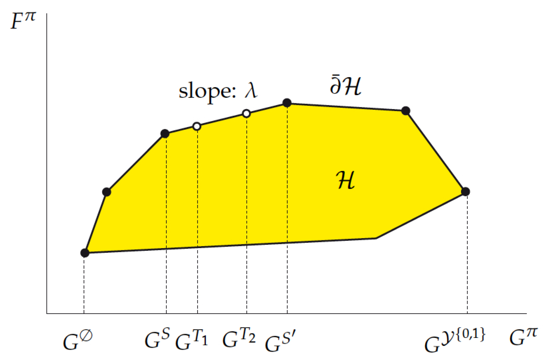
In order to illustrate and clarify such an approach, consider the concrete example of a certain restless bandit having state space Y = Y { 0 , 1 } = { 1 , 2 , 3 } that is discussed in (Sec. 2.2 of [34]) For such a project, Figure 1, in that paper, plots the achievable resource-reward performance region H , with points ( G S , F S ) being labeled by their active sets S.
The fact that such a project is indexable is apparent from the structure of the upper boundary of H ,
¯ H ( G , F ) H : F ˜ F for every ( G ˜ , F ˜ ) H having G ˜ = G ,
as this is determined from left to right by an increasing nested family of adjacent active sets connecting to Y { 0 , 1 } : F = , { 1 } , { 1 , 2 } , { 1 , 2 , 3 } . Thus, the Whittle indices of the states are given by the successive slopes measuring the marginal reward versus resource trade-off rates:
λ 1 * = F { 1 } F G { 1 } G λ 2 * = F { 1 , 2 } F { 1 } G { 1 , 2 } G { 1 } λ 3 * = F { 1 , 2 , 3 } F { 1 , 2 } G { 1 , 2 , 3 } G { 1 , 2 } .
In this example, the geometry of the top-down adaptive-greedy algorithm AG F corresponds to traversing the upper boundary ¯ H from left to right, proceeding, at each step, by augmenting the current active set by a new state in a locally greedy fashion, as the slopes in (26) are equivalently formulated as
λ 1 * = f 1 g 1 λ 2 * = f 2 { 1 } g 2 { 1 } λ 3 * = f 3 { 1 , 2 } g 3 { 1 , 2 } .
The insights that are conveyed by such an example extend to the general setting of concern herein, as elucidated in Niño-Mora [31,32,34]. Thus, the indexability of a project is recast as a property of the upper boundary ¯ H of region H , whereby it is determined by a nested active-set family as in the example. Note that the equivalence between the geometric slopes in (27) and the marginal productivity rates (26) in follow from (19) and (20) or, more precisely, from the corresponding relations for the averaged metrics,
G S \ { y } = G S g y S x y 0 , S \ { y } , y S G S { y } = G S + g y S x y 1 , S { y } , y Y { 0 , 1 } \ S ,
and
F S \ { y } = F S f y S x y 0 , S \ { y } , y S F S { y } = F S + f y S x y 1 , S { y } , y Y { 0 , 1 } \ S ,
where x y a , π is the state-action occupancy measure that is obtained by drawing the initial state according to the probabilities p y . Thus, assuming condition (i) in Theorem 1(a), we have, for S F ,
f y S g y S = F S F S \ { y } G S G S \ { y } , y S , S \ { y } F F S { y } F S G S { y j } G S , y Y { 0 , 1 } \ S , S { y } F .
Such relations allow for us to reformulate the adaptive-greedy algorithm AG F in Algorithm 1 into the geometrically intuitive form that is shown in Algorithm 2. Such a reformulation clarifies that this algorithm seeks to traverse, from left to right, the upper boundary ¯ H , proceeding at each step by augmenting the current active set by a new state in a locally greedy fashion, while only using active sets in F .
We next proceed to establish a number of preliminary results, on which the proof of Theorem 1 will draw. The first shows that the family of optimal active sets for the λ -price problem is a lattice that contains its intervals.
Lemma 4.
If S and S are optimal active sets for (22), then so is any S satisfying S S S S S .
Proof. 
The result is an immediate property of the DP Equations (11) characterizing the optimal stationary deterministic policies (i.e., the optimal active sets) for the λ -price problem. □
The following result shows that, under condition (i) in Theorem 1(a), resource consumption metric G S is strictly increasing relative to active-set inclusion in the domain S F .
Lemma 5.
Suppose that condition (i) in Theorem 1(a) holds. Then, G S < G S for S S , S , S F .
Proof. 
The result follows immediately from the formulation of such a condition (i) in (17), along with the assumption of positive initial state probabilities p y > 0 for y Y . □
The next result establishes, under conditions (i) and (ii) in Theorem 1(a), the non-degeneracy of the extreme points of H in upper boundary ¯ H , showing that each is achieved by a unique active set in F .
Lemma 6.
Suppose that conditions (i) and (ii) in Theorem 1(a) hold. Then, for every ( G * , F * ) ¯ H that is an extreme point of H , there exists a unique active set S * F achieving it, i.e., with ( G * , F * ) = ( G S , F S ) .
Proof. 
Because ( G * , F * ) is an extreme point of H in ¯ H , there exists a resource price λ * , such that ( G * , F * ) is the unique solution to the LP problem (24) for λ = λ * . Now, condition (ii) in Theorem 1 ensures that there exists an active set S * F that is optimal for λ * -price problem (22), i.e., such that ( G * , F * ) = ( G S * , F S * ) . Let us argue, by contradiction, that such an active set is unique, assuming that there exists a different active set S * * F , for which ( G * , F * ) = ( G S * * , F S * * ) . Then, by Assumption 2(iii) and Lemma 4, both S * S * * and S * S * * would belong in F and be optimal for the λ * -price problem. Therefore,
( G * , F * ) = ( G S * , F S * ) = ( G S * S * * , F S * S * * ) = ( G S * S * * , F S * S * * ) .
Now, since it is assumed that S * S * * , there are two cases to consider: in the first case, if it were S * S * * , then it would be S * S * * S * S * S * * and, hence, by Lemma 5, G S * S * * < G S * < G S * S * * , which contradicts (31). In the second case, if it were S * * S * , then it would be S * S * * S * * S * S * * and, hence, by Lemma 5, G S * S * * < G S * * < G S * S * * , which again contradicts (31). Therefore, there cannot exist such an S * * , which completes the proof. □
We can now prove Theorem 1.
Proof of Theorem 1.
(a) We will show that the project is F -indexable by using the geometric characterization of indexability that is reviewed in the present section. Namely, by showing that the upper boundary ¯ H is determined by an increasing nested family of adjacent active sets in F connecting ∅ to Y { 0 , 1 } . We refer the reader to the plot shown in Figure 1 for a geometric illustration of the following arguments.
Let us start by showing that the extreme points of H , which determine ¯ H , are attained, from left to right, by a unique increasing chain of active sets in F —not necessarily adjacent. Thus, consider two adjacent extreme points of H in ¯ H , i.e., joined by a line segment in ¯ H . By Lemma 6, there exist two unique and distinct active sets S , S F , whose performance points ( G S , F S ) and ( G S , F S ) achieve such extreme points, where we assume, without loss of generality, that G S < G S . We will show that it must be S S . Letting λ = ( F S F S ) / ( G S G S ) be the slope of the line segment joining such extreme points we have that both S and S solve the λ -price problem and, hence, by Lemma 4, so do S S and S S . Now, from the stated properties of S and S , it follows that points ( G S S , F S S ) and ( G S S , F S S ) must lie in the line segment joining ( G S , F S ) and ( G S , F S ) and, hence, G S S , G S S [ G S , G S ] . Further, since, by Assumption 2(iii) S S , S S F , Lemma 5 gives that G S S G S and G S G S S . Therefore,
G S = G S S = G S S = G S .
We next argue, by contradiction, that S S : if such were not the case, i.e., S S , then it would follow that S S S S S and, hence, by Lemma 5, G S S < G S < G S S , contradicting (32).
Let us next show that, if any two adjacent extreme points ( G S , F S ) and ( G S , F S ) in ¯ H , with G S < G S , are determined by active sets S S in such a chain that are not adjacent, they can be connected from left to right by points in ¯ H that are attained by an increasing chain of adjacent active sets in F . On the one hand, Assumption 2(ii) ensures the existence of an increasing chain of active sets in F that are adjacent and connect S to S : S = T 0 T 1 T k 1 T k = S . On the other hand, if λ = ( F S F S ) / ( G S G S ) is the slope of the line segment joining such extreme points, then we have that both S and S solve the λ -price problem and, hence, by Lemma 4, so does every intermediate active set T 1 , , T k 1 in such a chain. Hence, Lemma 5 ensures that G S < G T 1 < < G T k 1 < G S , as required.
In order to establish F -indexability, it only remains to show that the leftmost (resp. rightmost) extreme point of H in ¯ H is that attained by active set S = (resp. S = Y { 0 , 1 } ). This follows from Assumption 2(i), condition (ii) in Theorem 1(a), and Lemma 5 (ensuring that G < G S < G Y { 0 , 1 } for S F , S Y { 0 , 1 } ).
Having established F -indexability, the result that algorithm AG F computes the project’s Whittle index follows immediately from the algorithm’s geometric interpretation, as revealed by its reformulation in Algorithm 2.
(b) Suppose now that the project is indexable. Then, ¯ H is determined by some increasing chain of adjacent active sets connecting ∅ to Y { 0 , 1 } : S 0 = S 1 S N = Y { 0 , 1 } . Letting F { S 0 , S 1 , , S N } , it is readily seen that such an active-set family satisfies conditions (i) and (ii) in part (a). This completes the proof. □

4. Application to Projects with Setup Delays and Costs

This section deploys the framework and results above on restless bandit indexation in our motivating model: the restless bandit reformulation of a non-restless bandit with setup costs and delays (and no setdown penalties: cf. Section 2.1), as discussed in Section 2. The project label m is dropped thereafter from the notation.
In this reformulation, all of the augmented states are controllable, i.e., Y = Y { 0 , 1 } , and an active-state subset of the augmented state space Y representing a stationary deterministic policy is given by specifying the original-state subsets S 0 , S 1 X , such that the project is engaged when it was rested (resp. engaged) previously if the state X ( t ) belongs to S 0 (resp. in S 1 ). We will denote such an active set/policy, as in [27], by 
S 0 S 1 { 0 } × S 0 { 1 } × S 1 Y .
We next address the issue of guessing an appropriate family F of active sets S 0 S 1 , which contains optimal active sets for the λ -price problem of concern (cf. (10)), which is now formulated as
maximize π Π F ( a , i ) π G ( a , i ) π ,
where F ( a , i ) π and G ( a , i ) π are the reward and resource (work) metrics that are given by
F ( a , i ) π E ( a , i ) π k = 0 R Y ( t ) a ( t ) β t k and G ( a , i ) π E ( a , i ) π k = 0 Q Y ( t ) a ( t ) β t k .
The intuition that, under Assumption 1, if engaging the project is optimal when it was not set up, then engaging it should also be optimal when it was set up, leads us to posit the following choice of F :
F S 0 S 1 : S 0 S 1 X .
Such an F represents a family of policies that satisfies Assumption 2. If S 0 S 1 , policy S 0 S 1 F has the hysteresis region S 1 \ S 0 , i.e., when the original state X ( t ) lies in S 1 \ S 0 the policy sticks to the previously chosen action. We will seek to prove indexability with respect to such a family of policies, i.e., F -indexability.
Note that the marginal work, reward, and productivity metrics defined in general by (12)–(15) now take the form
g ( a , i ) S 0 S 1 G ( a , i ) 1 , S 0 S 1 G ( a , i ) 0 , S 0 S 1 ,
f ( a , i ) S 0 S 1 F ( a , i ) 1 , S 0 S 1 F ( a , i ) 0 , S 0 S 1 ,
and, for g ( a , i ) S 0 S 1 0 ,
λ ( a , i ) S 0 S 1 f ( a , i ) S 0 S 1 g ( a , i ) S 0 S 1 .
We next adapt to the present setting the general top-down adaptive-greedy algorithm AG F in Algorithm 1, which yields the algorithm in Algorithm 3, where n | X | is now the number of project states in the non-restless formulation. The output of the algorithm has been decoupled, noting that, at every step, the algorithm expands the current active set S 0 k 0 1 S 1 k 1 1 by adding a state that can be either of the form ( 0 , i 0 k 0 ) or ( 1 , i 1 k 1 ) . Thus, instead of using a single counter k, ranging from 0 to 2 n , two counters 1 k 0 k 1 n are used, with such counters being related by k = k 0 + k 1 1 . Henceforth, we use a more algorithm-like notation, writing, e.g., λ ( 0 , j ) S 0 k 0 1 S 1 k 1 1 as λ ( 0 , j ) ( k 0 1 , k 1 1 ) . Note that the active sets S 0 k 0 and S 1 k 1 that are generated in the algorithm are given by S 0 k 0 = { i 0 1 , , i 0 k 0 } and S 1 k 1 = { i 1 1 , , i 1 k 1 } , and satisfy S 0 k 0 S 1 k 1 , for 1 k 0 k 1 n , consistently with (35). Thus, the algorithm produces a decoupled output consisting of two augmented-state strings strings ( 0 , i 0 k 0 ) and ( 1 , i 1 k 1 ) , which jointly span Y , along with corresponding switching and continuation index values λ ( 0 , i 0 k 0 ) * and λ ( 1 , i 1 k 1 ) * .
Algorithm 3: Adaptation of index algorithm AG F to the present model.
  Output: ( 0 , i 0 k 0 ) , λ ( 0 , i 0 k 0 ) * k 0 = 1 n , ( 1 , i 1 k 1 ) , λ ( 1 , i 1 k 1 ) * k 1 = 1 n
   S 0 0 : = ; S 1 0 : = ; k 0 : = 1 ; k 1 : = 1
  while k 0 + k 1 2 n + 1 do
   if k 1 n choose j 1 max arg max λ ( 1 , j ) ( k 0 1 , k 1 1 ) : j X \ S 1 k 1 1
   if k 0 < k 1 choose j 0 max arg max λ ( 0 , j ) ( k 0 1 , k 1 1 ) : j S 1 k 1 1 \ S 0 k 0 1
   if k 1 = n + 1 or k 0 < k 1 n and λ ( 1 , j 1 max ) ( k 0 1 , k 1 1 ) < λ ( 0 , j 0 max ) ( k 0 1 , k 1 1 )
     i 0 k 0 : = j 0 max ; λ ( 0 , i 1 k 0 ) * : = λ ( 0 , i 1 k 0 ) ( k 0 1 , k 1 1 ) ; S 0 k 0 : = S 0 k 0 1 i 0 k 0 ; k 0 : = k 0 + 1
   else
     i 1 k 1 : = j 1 max ; λ ( 1 , i 1 k 1 ) * : = λ ( 1 , i 1 k 1 ) ( k 0 1 , k 1 1 ) ; S 1 k 1 : = S 1 k 1 1 { i 1 k 1 } ; k 1 : = k 1 + 1
   end { if }
  end { while }

4.1. Proving That F -Policies Are Optimal

We next aim to establish that condition (ii) in Theorem 1(a) is satisfied by the present model, i.e., that F -policies, i.e., those with active sets S 0 S 1 F that are defined by (35), suffice to solve the λ -price problem (33) for any price λ R . We will use the DP optimality equations that characterize the optimal value function V ( a , i ) * ( λ ) for problem (33), starting from each augmented state ( a , i ) Y : thus, for each original state i X ,
V ( 1 , i ) * ( λ ) = max β V ( 0 , i ) * ( λ ) , R i λ + β j X p i j V ( 1 , j ) * ( λ ) V ( 0 , i ) * ( λ ) = max β V ( 0 , i ) * ( λ ) , c i 1 ϕ i 1 β λ + ϕ i R i λ + β j X p i j V ( 1 , j ) * ( λ ) .
We start by showing that the optimal value function is non-negative.
Lemma 7.
V ( a , i ) * ( λ ) 0 .
Proof. 
Because no setdown penalties are assumed (cf. Section 2.1), a possible course of action incurring zero net reward is to set down the project and keep it that way, which yields the result. □
We can now prove the optimality of F -policies.
Lemma 8.
For every λ R , there exists an optimal active set S 0 S 1 F for λ-price problem (33).
Proof. 
Fix λ R and i X . It suffices to show that, if resting the project is optimal in state ( 1 , i ) , then it is also optimal doing so in state ( 0 , i ) . Let us formulate that hypothesis, as
β V ( 0 , i ) * ( λ ) R i λ + β j X p i j V ( 1 , j ) * ( λ ) .
We aim to show that, then, it is optimal resting the project in state ( 0 , i ) , so
β V ( 0 , i ) * ( λ ) c i 1 ϕ i 1 β λ + ϕ i R i λ + β j X p i j V ( 1 , j ) * ( λ ) .
Consider first the case λ < 0 . We will argue, by contradiction, that hypothesis (40) then cannot hold, i.e., it cannot be optimal to rest the project once it is active. Drawing on non-restless bandit theory, note that, when the project is active, it is optimal to rest it only if it ever reaches an original state j X at which λ λ j * , where λ j * is the original (non-restless) bandit’s Gittins index. Assumption 1(ii) now assures us that λ j * 0 for each j X , and, therefore, it is optimal to keep the project active forever.
Next, consider the case λ 0 . Then, the following chain of inequalities holds:
β V ( 0 , i ) * ( λ ) R i λ + β j X p i j V ( 1 , j ) * ( λ ) c i 1 ϕ i 1 β λ + ϕ i R i λ + β j X p i j V ( 1 , j ) * ( λ ) ,
where the fact that the second inequality holds is apparent by reformulating it as
( 1 ϕ i ) ( R i + β j X p i j V ( 1 , j ) * ( λ ) ) c i β 1 ϕ 1 β λ ,
and noting that Assumption 1(ii) and Lemma 7, ensure that the latter inequality left-hand side is non-negative, and, further, Assumption 1(i) and λ 0 ensure non-positivity of its right-hand side. This completes the proof. □

4.2. Work Metric Analysis and F -Indexability Proof

We now consider how to calculate work and marginal work metrics G ( a , i ) S 0 S 1 and g ( a , i ) S 0 S 1 , by relating them to the corresponding metrics G i S and g i S for the underlying non-restless project. We will further use such analyses to establish that condition (i) in Theorem 1(a) holds for the model of concern, thus allowing for us to apply such a theorem.
For each S X , the G i S are characterized by the unique solution to the evaluation equations
G i S = 1 + β j S p i j G j S if i S 0 otherwise .
Further, the marginal work metric g i S is evaluated by
g i S G i 1 , S G i 0 , S = 1 + β j X p i j G j S β G i S = ( 1 β ) G i S if i S 1 + β j S p i j G j S otherwise .
Note that (41) and (42) imply that
g i S > 0 , i N .
We now go back to the project’s restless bandit reformulation. The next result, whose proof is omitted, as it is immediate, gives the evaluation equations for work metric G ( a , i ) S 0 S 1 under a given active set.
Lemma 9.
For S 0 S 1 F ,
G ( 0 , i ) S 0 S 1 = 1 ϕ i 1 β + ϕ i G ( 1 , i ) S 0 S 1 if i S 0 0 otherwise and G ( 1 , i ) S 0 S 1 = 1 + β j X p i j G ( 1 , j ) S 0 S 1 if i S 1 0 otherwise .
The following result represents work metric G ( a , i ) S 0 S 1 in terms of the G j S .
Lemma 10.
For S 0 S 1 F :
(a)
G ( a , i ) S 0 S 1 = G i S 1 = 0 , for a { 0 , 1 } , i X \ S 1 .
(b)
G ( 1 , i ) S 0 S 1 = G i S 1 , for i S 1 .
(c)
G ( 0 , i ) S 0 S 1 = ( 1 ϕ i ) / ( 1 β ) + ϕ i G i S 1 , for i S 0 .
(d)
G ( 0 , i ) S 0 S 1 = 0 , for i S 1 \ S 0 .
Proof. 
(a) The result follows readily from the definition of S 0 S 1 .
(b) For i S 1 , we have
G ( 1 , i ) S 0 S 1 = 1 + β j S 1 p i j G ( 1 , j ) S 0 S 1 + β j X \ S 1 p i j G ( 1 , j ) S 0 S 1 = 1 + β j S 1 p i j G ( 1 , j ) S 0 S 1 ,
while using Lemma 9 and part (a). Thus, the G ( 1 , i ) S 0 S 1 satisfy the equations in (41) characterizing the G i S 1 for i S 1 , which gives the result.
(c) We have, for i S 0 ,
G ( 0 , i ) S 0 S 1 = 1 ϕ i 1 β + ϕ i G ( 1 , i ) S 0 S 1 = 1 ϕ i 1 β + ϕ i G i S 1 ,
using Lemma 9, the inclusion S 0 S 1 , and (a, b).
(d) The result follows readily from the definition of S 0 S 1 . □
Concerning the marginal work metric g ( a , i ) S 0 S 1 , (36) and Lemma 9, they readily give that
g ( 1 , i ) S 0 S 1 = 1 + β j X p i j G ( 1 , j ) S 0 S 1 β G ( 0 , i ) S 0 S 1 g ( 0 , i ) S 0 S 1 = 1 ϕ i 1 β + ϕ i 1 + β j X p i j G ( 1 , j ) S 0 S 1 β G ( 0 , i ) S 0 S 1 .
The following result represents marginal work metric g ( a , i ) S 0 S 1 in terms of the g j S .
Lemma 11.
For every a { 0 , 1 } , S 0 S 1 F :
(a)
g ( 1 , i ) S 0 S 1 = g i S 1 , for i X \ S 1 .
(b)
g ( 0 , i ) S 0 S 1 = 1 ϕ i 1 β + g i S 1 , for i X \ S 1 .
(c)
g ( 1 , i ) S 0 S 1 = 1 β ϕ i 1 β g i S 1 β 1 ϕ i 1 β ϕ i , for i S 0 .
(d)
g ( 0 , i ) S 0 S 1 = 1 ϕ i + ϕ i g i S 1 , for i S 0 .
(e)
g ( 1 , i ) S 0 S 1 = g i S 1 1 β , for i S 1 \ S 0 .
(f)
g ( 0 , i ) S 0 S 1 = 1 ϕ i 1 β + ϕ i 1 β g i S 1 , for i S 1 \ S 0 .
Proof. 
(a) We have, for i X \ S 1 ,
g ( 1 , i ) S 0 S 1 = 1 + β j X p i j G ( 1 , j ) S 0 S 1 β G ( 0 , i ) S 0 S 1 = 1 + β j S 1 p i j G j S 1 = g i S 1 ,
using (44), Lemma 10(a,b), and (42).
(b) We can write, for i X \ S 1 ,
g ( 0 , i ) S 0 S 1 = 1 ϕ i 1 β + ϕ i 1 + β j X p i j G ( 1 , j ) S 0 S 1 β G ( 0 , j ) S 0 S 1 = 1 ϕ i 1 β + ϕ i 1 + β j S 1 p i j G j S 1 = 1 ϕ i 1 β + ϕ i g i S 1 ,
while using (44), Lemma 10(a,b), and (42).
(c) We have, for i S 0 ,
g ( 1 , i ) S 0 S 1 = G ( 1 , i ) S 0 S 1 β G ( 0 , i ) S 0 S 1 = G i S 1 β 1 ϕ i 1 β + ϕ i G i S 1 = ( 1 β ϕ i ) G i S 1 β 1 ϕ i 1 β = 1 β ϕ i 1 β g i S 1 β 1 ϕ i 1 β ϕ i ,
using (44), S 0 S 1 , Lemma 9, Lemma 10(b,c), and (42).
(d) We obtain, for i S 0 ,
g ( 0 , i ) S 0 S 1 = 1 ϕ i 1 β + ϕ i G ( 1 , i ) S 0 S 1 β G ( 0 , i ) S 0 S 1 = 1 ϕ i 1 β + ϕ i G i S 1 β 1 ϕ i 1 β + ϕ i G i S 1 = 1 ϕ i + ϕ i ( 1 β ) G i S 1 = 1 ϕ i + ϕ i g i S 1 ,
while using Lemma 9, S 0 S 1 , Lemma 10(b,c), and (42).
(e) We have, for i S 1 \ S 0 ,
g ( 1 , i ) S 0 S 1 = G ( 1 , i ) S 0 S 1 β G ( 0 , i ) S 0 S 1 = G i S 1 = g i S 1 1 β ,
using (44), Lemma 9, Lemma 10(d), and (42).
(f) We have, for i S 1 \ S 0 ,
g ( 0 , i ) S 0 S 1 = 1 ϕ i 1 β + ϕ i G ( 1 , i ) S 0 S 1 = 1 ϕ i 1 β + ϕ i G i S 1 = 1 ϕ i 1 β + ϕ i 1 β g i S 1 ,
using (44), Lemma 9, Lemma 10(b), and (42). □
It must be now remarked that, at the corresponding point in the analysis of [27]—for the case with no setup delays ϕ i 1 —one could establish the positivity of the marginal work metric, i.e., g ( a , i ) S 0 S 1 > 0 for ( a , i ) Y , S 0 S 1 F , which is the first PCL-indexability condition and it implies the less stringent condition (i) in Theorem 1(a). However, here, it is apparent from Lemma 11(c) that, for i S 0 , g ( 1 , i ) S 0 S 1 can be negative for β that is close to 1. This is why we cannot use here the same line of argument that is given in [27] to show indexability.
As mentioned above, we will use, instead, for such a purpose, Theorem 1(a). The following result shows that condition (i) in that theorem holds for the model of concern.
Lemma 12.
For S 0 S 1 F ,
g ( a , i ) S 0 S 1 > 0 , ( a , i ) S 0 S 1 , S 0 S 1 \ { ( a , i ) } F g ( a , i ) S 0 S 1 > 0 , ( a , i ) Y \ S 0 S 1 , S 0 S 1 { ( a , i ) } F .
Proof. 
First, consider the case S 0 S 1 = . Then, using Lemma 11(a–d), along with g i 1 , gives that, for i X ,
g ( 1 , i ) = g i = 1 > 0 , g ( 0 , i ) = 1 ϕ i 1 β + g i = 1 ϕ i 1 β + 1 > 0 .
Now, consider the case S 0 S 1 = X X = Y . Then, again using Lemma 11(a–d) along with g i X 1 gives that, for i X ,
g ( 1 , i ) X X = 1 β ϕ i 1 β g i X β 1 ϕ i 1 β ϕ i = 1 > 0 , g ( 0 , i ) X X = 1 ϕ i + ϕ i g i X = 1 > 0 .
Finally, consider S 0 S 1 F , which is different from and X X . Then, Lemma 11 and (35) imply that it could only happen that marginal work metric g ( a , i ) S 0 S 1 be negative if a = 1 and i S 0 . However, such a case is not included in the required conditions, since ( 1 , i ) S 0 S 1 (due to S 0 S 1 ), yet S 0 S 1 \ { ( 1 , i ) } = S 0 S 1 \ { i } F (since i S 0 S 1 \ { i } ). This completes the proof. □
We are now ready to deploy Theorem 1(a) in the present model.
Proposition 1.
The present restless bandit model is F -indexable and Algorithm 3 computes its Whittle index.
Proof. 
Lemmas 8 and 12 show that conditions (i) and (ii) in Theorem 1(a) hold, respectively, which implies the result. □

4.3. The AT Index Is the Whittle Index

We next use the results above in order to prove the identity between the Whittle index and the AT index. We will reformulate the AT index formulae in (7)–(8) while using active sets S X , rather than stopping times τ . Thus, we can reformulate the continuation and switching AT indices, as
λ ( 1 , i ) AT max S X : i S F i S G i S ,
and
λ ( 0 , i ) AT max S X : i S c i + ϕ i F i S 1 ϕ i 1 β + ϕ i G i S .
Recall that we denote the Whittle index by λ ( a , i ) * .
Proposition 2.
For i X , λ ( 1 , i ) * = λ ( 1 , i ) AT and λ ( 0 , i ) * = λ ( 0 , i ) AT .
Proof. 
We start by showing that λ ( 1 , i ) * = λ ( 1 , i ) AT , while using the equivalences
λ λ ( 1 , i ) * resting the project in ( 1 , i ) is optimal for problem ( 33 ) 0 max S 0 S 1 X : i S 1 F ( 1 , i ) S 0 S 1 λ G ( 1 , i ) S 0 S 1 λ max S 0 S 1 X : i S 1 F ( 1 , i ) S 0 S 1 G ( 1 , i ) S 0 S 1 λ max i S 1 X F i S 1 G i S 1 = λ ( 1 , i ) AT ,
drawing on the project’s F -indexability (Proposition 1), and so, if resting the project iin ( 1 , i ) is optimal, then resting it in ( 0 , i ) is also optimal, together with Lemmas 10(b) and 14(b).
We next prove that λ ( 0 , i ) * = λ ( 0 , i ) AT , through the chain of equivalences
λ λ ( 0 , i ) * resting the project in ( 0 , i ) is optimal for ( 33 ) 0 max S 0 S 1 X : i S 0 F ( 0 , i ) S 0 S 1 λ G ( 0 , i ) S 0 S 1 λ max S 0 S 1 X : i S 0 F ( 0 , i ) S 0 S 1 G ( 0 , i ) S 0 S 1 λ max S 1 X : i S 1 c i + ϕ i F i S 1 1 ϕ i 1 β + ϕ i G i S 1 = λ ( 0 , i ) AT ,
drawing on the result that the project is F -indexable, together with Lemmas 10(c) and 14(c). □

4.4. Reward Metric Analysis

We proceed by considering how to calculate the reward and marginal reward metrics F ( a , i ) S 0 S 1 and f ( a , i ) S 0 S 1 , by relating them to the metrics F i S and f i S for the corresponding non-restless project with no setup penalties.
For every active set S X , the reward metric F i S is determined by the evaluation equations
F i S = R i + β j S p i j F j S if i S 0 otherwise ,
and the marginal reward metric is given by
f i S F i 1 , S F i 0 , S = R i + β j S p i j F j S β F i S = ( 1 β ) F i S if i S R i + β j S p i j F j S otherwise .
Going back to the semi-Markov restless bandit reformulation, the following result shows the evaluation equations for the reward metrics F ( a , i ) S 0 S 1 , for an active set S 0 S 1 F .
Lemma 13.
F ( a , i ) S 0 S 1 = R i + β j X p i j F ( 1 , j ) S 0 S 1 if a = 1 , i S 1 c i + ϕ i R i + β j X p i j F ( 1 , j ) S 0 S 1 if a = 0 , i S 0 β F ( 0 , i ) S 0 S 1 otherwise .
The following result formulates the reward metric F ( a , i ) S 0 S 1 , in terms of the F i S ’s.
Lemma 14.
For S 0 S 1 F :
(a)
F ( a , i ) S 0 S 1 = 0 = F i S 1 , for a { 0 , 1 } , i X \ S 1 .
(b)
F ( 1 , i ) S 0 S 1 = F i S 1 , for i S 1 .
(c)
F ( 0 , i ) S 0 S 1 = c i + ϕ i F i S 1 , for i S 0 .
(d)
F ( 0 , i ) S 0 S 1 = 0 = F i S 0 , for i S 1 \ S 0 .
Proof. 
(a) This part follows from the definition of S 0 S 1 .
(b) We have, for i S 1 ,
F ( 1 , i ) S 0 S 1 = R i + β j S 1 p i j F ( 1 , j ) S 0 S 1 + β j X \ S 1 p i j F ( 1 , j ) S 0 S 1 = R i + β j S 1 p i j F ( 1 , j ) S 0 S 1 ,
while using Lemma 13 and part (a). Thus, the F ( 1 , i ) S 0 S 1 ’s, for i S 1 , satisfy (47), which yields the result.
(c) We can write, for i S 0 ,
F ( 0 , i ) S 0 S 1 = c i + ϕ i R i + β j S 1 p i j F ( 1 , j ) S 0 S 1 = c i + ϕ i F i S 1 ,
using parts (a, b), Lemma 13, and (47).
(d) The result follows from the definition of S 0 S 1 . □
Concerning the marginal reward metric f ( a , i ) S 0 S 1 , we obtain, from (37) and Lemma 13, that
f ( 1 , i ) S 0 S 1 = R i + β j X p i j F ( 1 , j ) S 0 S 1 β F ( 0 , i ) S 0 S 1 f ( 0 , i ) S 0 S 1 = c i + ϕ i R i + β j X p i j F ( 1 , j ) S 0 S 1 β F ( 0 , i ) S 0 S 1 .
The following result represents the marginal reward f ( a , i ) S 0 S 1 in terms of the f j S .
Lemma 15.
For S 0 S 1 F :
(a)
f ( 1 , i ) S 0 S 1 = f i S 1 , for i X \ S 1 .
(b)
f ( 0 , i ) S 0 S 1 = c i + f i S 1 , for i X \ S 1 .
(c)
f ( 1 , i ) S 0 S 1 = β c i + 1 β ϕ i 1 β f i S 1 , for i S 0 .
(d)
f ( 0 , i ) S 0 S 1 = ( 1 β ) c i + ϕ i f i S 1 , for i S 0 .
(e)
f ( 1 , i ) S 0 S 1 = f i S 1 1 β , for i S 1 \ S 0 .
(f)
f ( 0 , i ) S 0 S 1 = c i + ϕ i f i S 1 1 β , for i S 1 \ S 0 .
Proof. 
(a) We have, for i X \ S 1 ,
f ( 1 , i ) S 0 S 1 = R i + β j X p i j F ( 1 , j ) S 0 S 1 F ( 1 , i ) S 0 S 1 = R i + β j S 1 p i j F j S 1 = f i S 1 ,
using (49), Lemmas 13 and 14(a,b), (47), and (48).
(b) We can write, for i X \ S 1 ,
f ( 0 , i ) S 0 S 1 = c i + ϕ i 1 + β j X p i j F ( 1 , j ) S 0 S 1 β F ( 0 , j ) S 0 S 1 = c i + ϕ i 1 + β j S 1 p i j F j S 1 = c i + ϕ i f i S 1 ,
using (49), (48), and Lemma 14(a,b).
(c) We have, for i S 0 ,
f ( 1 , i ) S 0 S 1 = F ( 1 , i ) S 0 S 1 β F ( 0 , i ) S 0 S 1 = F i S 1 β c i + ϕ i F i S 1 = β c i + ( 1 β ϕ i ) F i S 1 = β c i + 1 β ϕ i 1 β f i S 1 ,
using (49), S 0 S 1 , Lemmas 13 and 14(b,c), and (48).
(d) We can write, for i S 0 ,
f ( 0 , i ) S 0 S 1 = c i + ϕ i F ( 1 , i ) S 0 S 1 β F ( 0 , i ) S 0 S 1 = c i + ϕ i F i S 1 β c i + ϕ i F i S 1 = ( 1 β ) c i + ϕ i ( 1 β ) F i S 1 = ( 1 β ) c i + ϕ i f i S 1 ,
while using Lemmas 13 and 14(b,c), S 0 S 1 , and (48).
(e) We have, for i S 1 \ S 0 ,
f ( 1 , i ) S 0 S 1 = F ( 1 , i ) S 0 S 1 β F ( 0 , i ) S 0 S 1 = F i S 1 = f i S 1 1 β ,
using (49), Lemmas 13 and 14(d), and (48).
(f) We obtain, for i S 1 \ S 0 ,
f ( 0 , i ) S 0 S 1 = c i + ϕ i R i + β j N p i j F ( 1 , j ) S 0 S 1 β F ( 0 , i ) S 0 S 1 = c i + ϕ i F i S 1 = c i + ϕ i f i S 1 1 β ,
using (49), Lemmas 13 and 14(b), and (48). This completes the proof. □

5. Designing an Efficient Two-Stage Index Algorithm

This section draws on the above in order to develop an efficient index algorithm, which exploits special structure to simplify the one-stage adaptive-greedy algorithm in Algorithm 3, by decoupling the calculation of the continuation and switching indices into a two-stage method, for which an efficient implementation is provided.

5.1. Marginal Productivity Metric Analysis

We start by addressing the calculation of required marginal productivity metrics λ ( a , i ) S 0 S 1 in (38), also by relating them to metrics λ i S for the corresponding non-restless project without setup penalties, which are given by
λ i S f i S g i S , i X , S X .
The next result represents λ ( a , i ) S 0 S 1 in terms of the λ j S .
Lemma 16.
For S 0 S 1 F :
(a)
λ ( 1 , i ) S 0 S 1 = λ i S 1 , for i X \ S 1 .
(b)
λ ( 0 , i ) S 0 S 1 = c i + f i S 1 1 ϕ i 1 β + g i S 1 = g i S 1 1 ϕ i 1 β + g i S 1 λ i S 1 c i g i S 1 , for i X \ S 1 .
(c)
λ ( 1 , i ) S 0 S 1 = β c i + 1 β ϕ i 1 β f i S 1 1 β ϕ i 1 β g i S 1 β 1 ϕ i 1 β ϕ i = g i S 1 g i S 1 β 1 ϕ i 1 β ϕ i λ i S 1 + β ( 1 β ) 1 β ϕ i c i g i S 1 , for i S 0 such that g i S 1 β 1 ϕ i 1 β ϕ i .
(d)
λ ( 0 , i ) S 0 S 1 = ( 1 β ) c i + ϕ i f i S 1 1 ϕ i + ϕ i g i S 1 = ( 1 β ) c i + ϕ i g i S 1 λ i S 1 1 ϕ i + ϕ i g i S 1 , for i S 0 .
(e)
λ ( 1 , i ) S 0 S 1 = λ i S 1 , for i S 1 \ S 0 .
(f)
λ ( 0 , i ) S 0 S 1 = λ i S 1 1 β c i + 1 ϕ i λ i S 1 1 ϕ i + ϕ i g i S 1 , i S 1 \ S 0 .
Proof. 
All of the parts follow readily from (50), (38), and Lemmas 11 and 15. □

5.2. Simplified Version of the Index Algorithm

Using the above results allows for us to give a simplified and more explicit version of the index algorithm AG F in Algorithm 3, which is given in Algorithm 4. In it, we draw on Lemma 16(b,d) to formulate marginal productivity rates λ ( a , i ) S 0 S 1 in terms of the g j S and λ j S . Thus, the g j ( k 1 1 ) and λ j ( k 1 1 ) in the algorithm correspond to g ( 1 , j ) ( k 0 1 , k 1 1 ) and λ ( 1 , j ) ( k 0 1 , k 1 1 ) , respectively. Further, we use λ ( 0 , j ) ( 0 , k 1 1 ) (which denotes λ ( 0 , j ) S 0 0 S 1 k 1 1 ) in place of λ ( 0 , j ) ( k 0 1 , k 1 1 ) , drawing on Lemma 16(d). Note that such simplifications achieve significant savings in computer memory, since storage of quantities λ j ( k 1 1 ) and λ ( 0 , j ) ( 0 , k 1 1 ) entail one less dimension than storing of the λ ( 1 , j ) ( k 0 1 , k 1 1 ) and λ ( 0 , j ) ( k 0 1 , k 1 1 ) .
Algorithm 4: Simplified version of index algorithm AG F .
  Output: { ( 0 , i 0 k 0 ) , λ ( 0 , i 0 k 0 ) * } k 0 = 1 n , { ( 1 , i 1 k 1 ) , λ ( 1 , i 1 k 1 ) * } k 1 = 1 n
   S 0 0 : = ; S 1 0 : = ; k 0 : = 1 ; k 1 : = 1 ; compute { ( g i ( 0 ) , λ i ( 0 ) ) : i X }
  while k 0 + k 1 2 n + 2 do
   if k 1 n choose j 1 max arg max λ j ( k 1 1 ) : j X \ S 1 k 1 1
    λ ( 0 , j ) ( 0 , k 1 1 ) : = λ j ( k 1 1 ) 1 β c j + 1 ϕ j λ j ( k 1 1 ) 1 ϕ j + ϕ j g j ( k 1 1 ) , j S 1 k 1 1 \ S 0 k 0 1
   if k 0 < k 1 choose j 0 max arg max λ ( 0 , j ) ( 0 , k 1 1 ) : j S 1 k 1 1 \ S 0 k 0 1
   if k 1 = n + 1 or k 0 < k 1 n and λ j 1 max ( k 1 1 ) < λ j 0 max ( 0 , k 1 1 )
     i 0 k 0 : = j 0 max ; λ ( 0 , i 0 k 0 ) * : = λ ( 0 , i 0 k 0 ) ( 0 , k 1 1 ) ; S 0 k 0 : = S 0 k 0 1 { i 0 k 0 } ; k 0 : = k 0 + 1
   else
     i 1 k 1 : = j 1 max ; λ i 1 k 1 * : = λ i 1 k 1 ( k 1 1 ) ; S 1 k 1 : = S 1 k 1 1 { i 1 k 1 } ; k 1 : = k 1 + 1
    compute { ( g i ( k 1 ) , λ i ( k 1 ) ) : i X }
   end { if }
  end { while }

5.3. Two-Stage Implementation of the Index Algorithm

We next proceed to still further simplify the index algorithm in Algorithm 4, by decoupling it into two successive algorithms. The first stage of such a scheme computes the continuation index λ ( 1 , i ) * , which we saw above is just the Gittins index λ i * . We will need additional quantities as input to the second stage: the g j ( k 1 ) and λ j ( k 1 ) appearing in Algorithm 4.
In order to obtain such an index and the required additional quantities, consider the algorithmic scheme AG 1 in Algorithm 5, which is a variant of that in [8], reformulated as in [28]. For implementations, we can use algorithms that are provided in the latter paper, in particular the fast-pivoting algorithm with extended output, which has an ( 4 / 3 ) n 3 + O ( n 2 ) arithmetic-operation count.
Algorithm 5: Gittins-index algorithmic scheme AG 1 .
  Output: { i 1 k 1 } k 1 = 1 n , { λ j * : j X } , { ( g j ( k 1 ) , λ j ( k 1 ) ) : j S 1 k 1 } k 1 = 1 n
  set S 1 0 : = ; compute { ( g i ( 0 ) , λ i ( 0 ) ) : i X }
  for k 1 : = 1 to n do
   choose i 1 k 1 arg max λ i ( k 1 1 ) : i X \ S 1 k 1 1
    λ i 1 k 1 * : = λ i 1 k 1 ( k 1 1 ) ; S 1 k 1 : = S 1 k 1 1 { i 1 k 1 }
   compute { ( g i ( k 1 ) , λ i ( k 1 ) ) : i X }
  end
We next address the computation of the switching index in the second stage, once the Gittins index and required extra quantities have been computed. Consider algorithm AG 0 that is given in Algorithm 6, whose input is the output of algorithm AG 1 , and which returns a sequence of all the states i 0 k 0 in X , together with index values λ ( 0 , i 0 k 0 ) * . Note that such an algorithm is formulated in a form applying to the case of concern herein, with a positive setup delay at every state j, so ϕ j < 1 .
Algorithm 6: Switching-index algorithm AG 0 .
  ALGORITHM AG 0 :
  Input: { i 1 k 1 } k 1 = 1 n , { λ j * : j X } , { ( g j ( k 1 ) , λ j ( k 1 ) ) : j S 1 k 1 } k 1 = 1 n
  Output: { i 0 k 0 } k 0 = 1 n , { λ ( 0 , j ) * : j X }
   c ^ j : = 1 β 1 ϕ j c j , j X ; z j = ϕ j / ( 1 ϕ j ) ; S 0 0 : = ; S 1 0 : = ; k 0 : = 0
  for k 1 : = 1 to n do
    S 1 k 1 : = S 1 k 1 1 { i 1 k 1 } ; AUGMENT 1 : = false
    λ ( 0 , j ) ( 0 , k 1 ) : = λ j ( k 1 1 ) c ^ j + λ j ( k 1 1 ) 1 + z j g j ( k 1 1 ) , j S 1 k 1 \ S 0 k 0
   while k 0 < k 1 and not( AUGMENT 1 ) do
    choose j 0 max arg max λ ( 0 , j ) ( 0 , k 1 ) : j S 1 k 1 \ S 0 k 0
    if k 1 = n or λ i 1 k 1 * < λ ( 0 , j 0 max ) ( 0 , k 1 )
      i 0 k 0 + 1 : = j 0 max ; λ ( 0 , i 0 k 0 + 1 ) * : = λ ( 0 , i 0 k 0 + 1 ) ( 0 , k 1 )
      S 0 k 0 + 1 : = S 0 k 0 { i 0 k 0 + 1 } ; k 0 : = k 0 + 1
    else
      AUGMENT 1 : = true
    end { if }
   end { while }
  end { for }
We have the following result.
Proposition 3.
Algorithm AG 0 computes index λ ( 0 , i ) * in no more than ( 5 / 2 ) n 2 + O ( n ) operations.
Proof. 
The fact that algorithm AG 0 calculates the λ ( 0 , i ) * follows by noting that we have obtained it from algorithm AG F in Algorithm 4 simply by decoupling the calculation of the λ ( 0 , i ) * and the λ ( 1 , i ) * = λ i * .
As for the algorithm’s arithmetic-operation count, it is dominated by the statements
λ ( 0 , j ) ( 0 , k 1 ) : = λ j ( k 1 1 ) c ^ j + λ j ( k 1 1 ) 1 + z j g j ( k 1 1 ) , j S 1 k 1 \ S 0 k 0 ,
for k 1 = 2 , , n + 1 , each of which performs no more than 5 k 1 operations. This gives the maximum stated operation count. □

6. How Does the Index Depend on Switching Penalties?

We next present and discuss properties on the index dependence on the switching penalties, when considering the case where the latter are constant across states: c i c , d i d and ϕ i ϕ for i X . The notation below will make explicit the prevailing penalties, writing λ ( 1 , i ) * ( d , ψ ) , and λ ( 0 , i ) * ( c , d , ϕ , ψ ) .
We write, as λ i * 0 , the Gittins index, and as F i S 0 , the reward metric of the original project with no switching penalties. We will draw on the following expression for the switching index:
λ ( 0 , i ) * ( c , d , ϕ , ψ ) = max S X : i S H c , d , ϕ , ψ , F i S , G i S ,
where
H ( c , d , ϕ , ψ , F , G ) ( c + ϕ d ) + ϕ F + ( 1 β ) d G 1 ϕ ψ 1 β + ϕ ψ G .
Note that (51) uses the transformation that is considered in Section 2.1, together with the switching-index formulation in (46), while using the result that the original non-restless project’s reward metric with transformed rewards R ˜ j = ( R j + ( 1 β ) d ) / ψ , for j X , is F ˜ i S = ( F i S + ( 1 β ) d G i S ) / ψ .
We will further use the following preliminary result.
Lemma 17.
(a)
If S S X , then F i S F i S and G i S G i S .
(b)
If d + ψ c ϕ ψ F i X , then H ( c , d , ϕ , ψ , F , G ) is monotone increasing in F and in G.
Proof. 
(a) The results follows from the interpretation of work and reward metrics, using Assumption 1(ii) for the latter.
(b) This part follows from the following results:
F H ( c , d , ϕ , ψ , F , G ) = ϕ 1 ϕ ψ 1 β + ϕ ψ G > 0 and G H ( c , d , ϕ , ψ , F , G ) = ϕ d + ψ c ϕ ψ F 1 ϕ ψ 1 β + ϕ ψ G 2 > 0 .
 □
We have the following result.
Proposition 4.
(a)
λ ( 1 , i ) * ( d , ψ ) = ( λ i * + ( 1 β ) d ) / ψ .
(b)
If d + ψ c ϕ ψ F i X , then λ ( 0 , i ) * = ϕ λ i X ( 1 β ) c .
(c)
λ ( 0 , i ) * ( c , d , ϕ , ψ ) is convex and piecewise linear in ( c , d ) , decreasing in c and non-increasing in d.
(d)
For d + ψ c ϕ ψ F i X , or for c , d 0 small enough and R i > 0 , or for c = d = 0 , λ ( 0 , i ) * ( c , d , ϕ , ψ ) is convex and non-decreasing in ϕ and in ψ.
(e)
lim ϕ 0 λ ( 0 , i ) * ( c , d , ϕ , ψ ) = ( 1 β ) c .
(f)
λ ( 0 , i ) * ( c , d , ϕ , ψ ) = ϕ λ i N ( 1 β ) c + O ( ψ 2 ) , as ψ 0 .
Proof. 
(a) The result follows from noting that λ ( 1 , i ) * ( d , ψ ) is the Gittins index of the project with modified active rewards R ˜ j = ( R j + ( 1 β ) d ) / ψ (cf. Section 2.1), which is related to the project Gittins index λ i * (with unmodified rewards R j ) by the stated expression.
(b) Using Lemma 17(b) and λ i X = ( 1 β ) F i X , we obtain
λ ( 0 , i ) * ( c , d , ϕ , ψ ) = max ( F , G ) [ 0 , F i X ] × [ 0 , G i X ] H ( c , d , ϕ , ψ , F , G ) = H c , d , ϕ , ψ , F i X , G i X = ϕ λ i X ( 1 β ) c .
(c) The result follows by noting that (51) formulates λ ( 0 , i ) * ( c , d , ϕ , ψ ) as the maximum of linear functions in ( c , d ) that decrease in c and are non-increasing in d.
(d) Concerning the dependence on ϕ , when d + ψ c ϕ ψ F i X the result follows by (b). Furthermore,
ϕ H c , d , ϕ , ψ , F i S , G i S = 1 β F i S 1 ( 1 β ) G i S ( d + ψ c ) 1 ϕ ψ 1 ( 1 β ) G i S 2 0 2 ϕ 2 H c , d , ϕ , ψ , F i S , G i S , = 2 ( 1 β ) 1 ( 1 β ) G i S ψ 1 ϕ ψ 1 ( 1 β ) G i S 3 F i S 1 ( 1 β ) G i S ( d + ψ c ) 0 ,
where the inequalities hold for c , d small enough, using that R i > 0 so that F i S > 0 , and for c = d = 0 . Hence, λ ( 0 , i ) * ( c , d , ϕ , ψ ) is a maximum of convex non-decreasing functions, which is also convex non-decreasing.
The same argument can be applied to dependence on ψ , while using that
ψ H c , d , ϕ , ψ , F i S , G i S = ( 1 β ) 1 ( 1 β ) G i S ϕ 1 ϕ ψ 1 ( 1 β ) G i S 2 ϕ F i S c 1 1 β G i S ϕ d 2 ψ 2 H c , d , ϕ , ψ , F i S , G i S = 2 ( 1 β ) 1 ( 1 β ) G i S 2 ϕ 2 ( 1 ϕ ψ 1 ( 1 β ) G i S ) 3 ϕ F i S c 1 1 β G i S ϕ d .
Parts (e) and (f) follow straightforwardly. □
We conjecture that Lemma 4(c) should hold without the qualifications considered above.
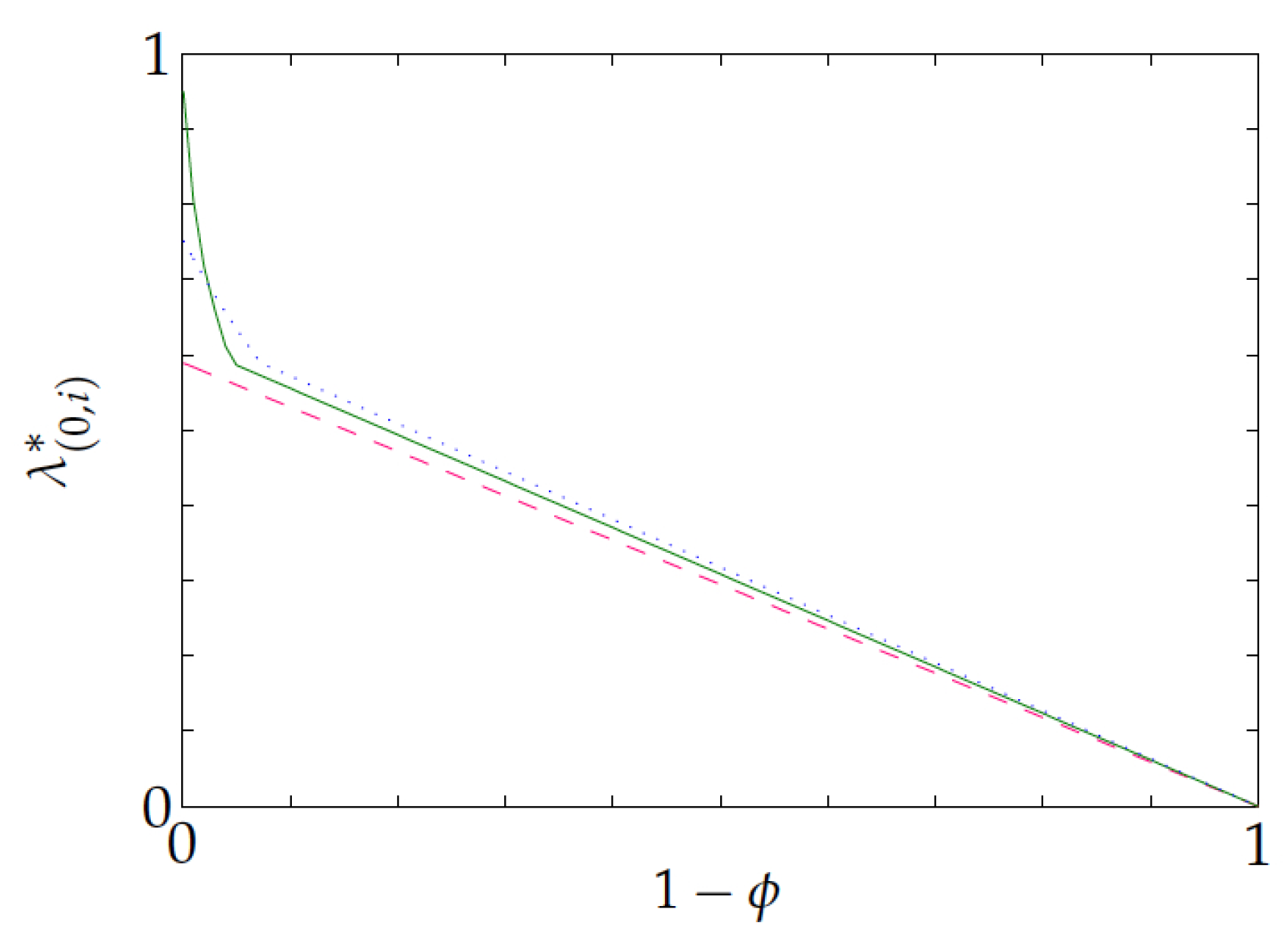
Now, consider the following examples to illustrate the results above. The first example concerns a three-state project with no setdown penalties or setup costs, setup delay transform ϕ , β = 0.95 ,
R = 0.7221 0.9685 0.1557 and P = 0.8061 0.1574 0.0365 0.1957 0.0067 0.7976 0.1378 0.5959 0.2663 .
Figure 2 plots the project’s switching index for each of the three states versus 1 ϕ . Note that each of the lines shown corresponds to one of the project states. The plot agrees with Proposition 4(d, e). It also illustrates that the relative ordering of states that is induced by the switching index can vary with ϕ .
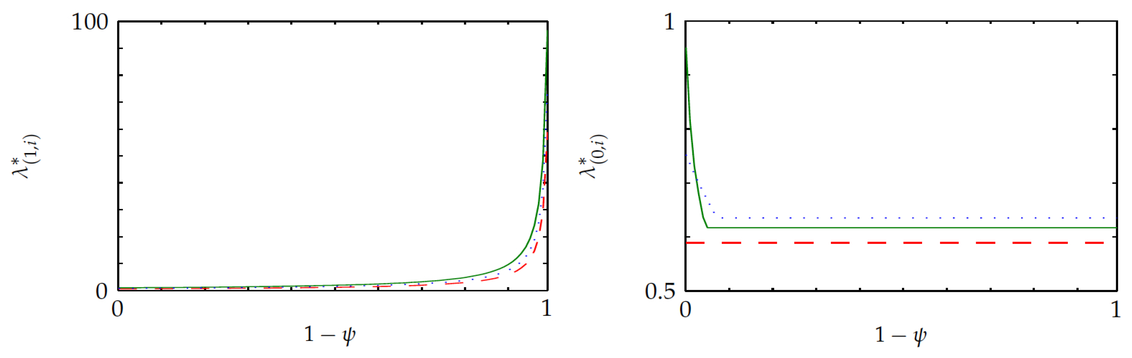
The following example is based on the same project, but with no setup delays and with setdown delay transform ψ . Figure 3 displays the continuation and switching indices for each of the three states versus 1 ψ . Note that each of the lines shown corresponds to one of the project states. The plots agree with Proposition 4(a,d,f). Note that the continuation index λ ( 1 , i ) * ( d , ψ ) increases to infinity as ψ vanishes, as the incentive of sticking to a project increases steeply as the setdown delay becomes larger. The plot for the switching index further shows that the relative ordering of states can vary with ψ .

7. Numerical Study

We next report on the results of a numerical study, which is based on MATLAB implementations of the algorithms that are discussed here developed by the author.
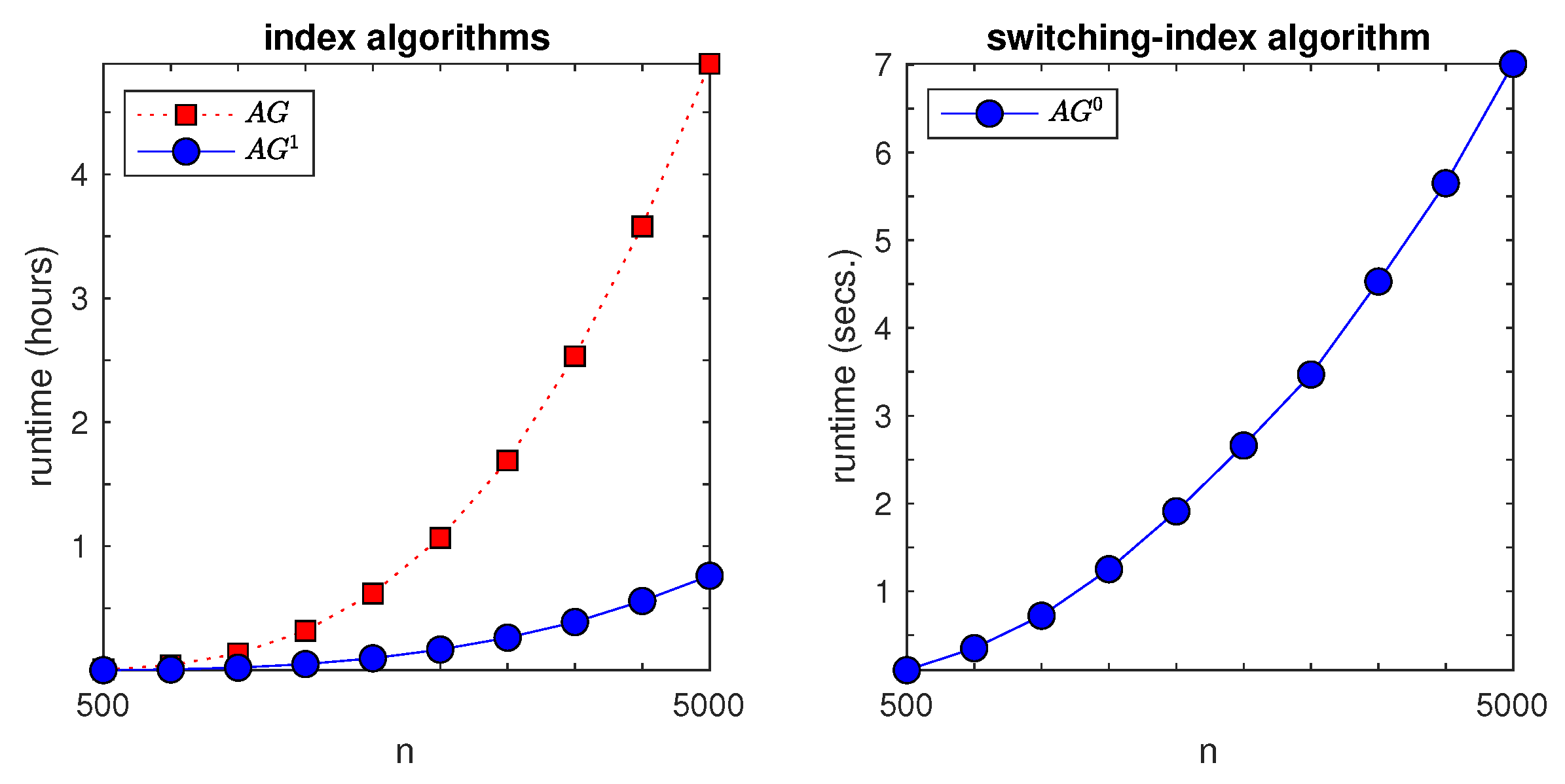
The first experiment addressed the runtime of the decoupled index computing method. A random project instance with setup delays and costs was randomly generated for each of the following numbers of states: n = 500 , 1000 , , 5000 . For each such n, the time to compute the continuation index and required extra quantities while using the fast-pivoting algorithm with extended output in [28] was recorded, as well as the time for computing the switching index by algorithm AG 0 , and the time for jointly computing both indices by using the simplex-based implementation that is given in [49] of the adaptive-greedy algorithm AG F . This experiment was run on a 2.8 GHz PC with 4 GB of memory.
Figure 4 shows the results. The left pane plots total runtimes (measured in hours) to compute both indices versus n. Red squares represent the AG F joint-computing scheme, and blue circles represent the two-stage scheme. We see that the latter attained approximately a fourfold speed-up over the former. The right pane plots runtimes (measured in seconds), for the switching index algorithm versus the number of states n. The timescale change from hours to seconds highlights the order-of-magnitude speed-up attained.
The following experiments were designed in order to evaluate the average relative performance of the Whittle index policy in randomly generated two- and three-project instances, both versus the optimal problem value, and versus the benchmark Gittins index policy, which does not take setups into account. For each problem instance, the optimal value was calculated by solving with the CPLEX LP solver the LP formulation of the DP optimality equations. The Whittle index and benchmark scheduling policies were evaluated by solving, with MATLAB, the appropriate systems of linear evaluation equations.
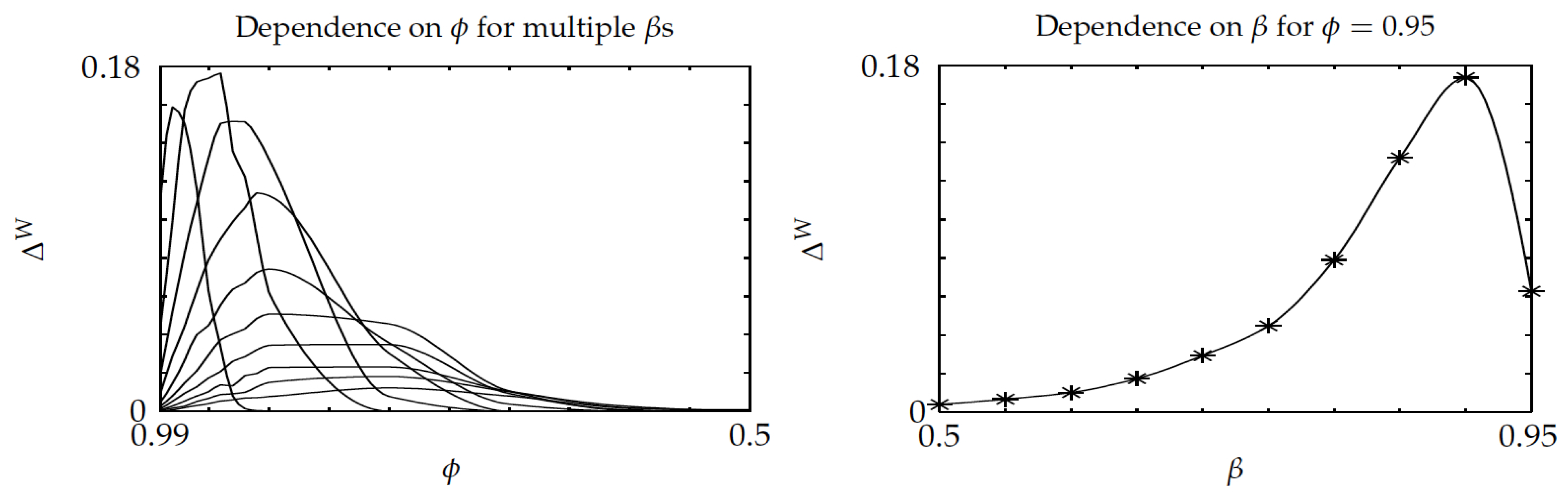
The second experiment was designed to assess the dependence of the relative performance of Whittle’s index policy for two-project instances on a constant setup-time transform ϕ and discount factor β —with no setdown penalties. A sample of 100 randomly generated instances with 10-state projects was obtained with MATLAB. In each instance, the parameters for each project were independently drawn: transition probabilities (by scaling a matrix with uniform entries) and uniform (between 0 and 1) active rewards. For every instance k = 1 , , 100 and parameters ( ϕ , β ) [ 0.5 , 0.99 ] × [ 0.5 , 0.95 ] —with a 0.1 grid—the optimal value V ( k ) , opt and the values of the Whittle index ( V ( k ) , W ) and benchmark ( V ( k ) , bench ) policies were calculated, together with the relative optimality of the Whittle index policy Δ ( k ) , W 100 ( V ( k ) , opt V ( k ) , W ) / | V ( k ) , opt | , and the optimality-gap ratio of the Whittle index over the benchmark policy ρ ( k ) , W , bench 100 ( V ( k ) , W V ( k ) , opt ) / ( V ( k ) , bench V ( k ) , opt ) . The latter were then averaged over the 100 instances for each ( c , β ) pair, in order to obtain the average values Δ W and ρ W , bench .
Values V ( k ) , opt , V ( k ) , W and V ( k ) , bench were computed, as follows. The corresponding value functions V ( ( a 1 , i 1 ) , ( a 2 , i 2 ) ) ( k ) , opt , V ( ( a 1 , i 1 ) , ( a 2 , i 2 ) ) ( k ) , W and V ( ( a 1 , i 1 ) , ( a 2 , i 2 ) ) ( k ) , bench were calculated. Subsequently, the values were calculated when considering that both projects start out being passive, as
V ( k ) , π 1 n 2 i 1 , i 2 N V ( ( 0 , i 1 ) , ( 0 , i 2 ) ) ( k ) , π , π { opt , W , bench } .
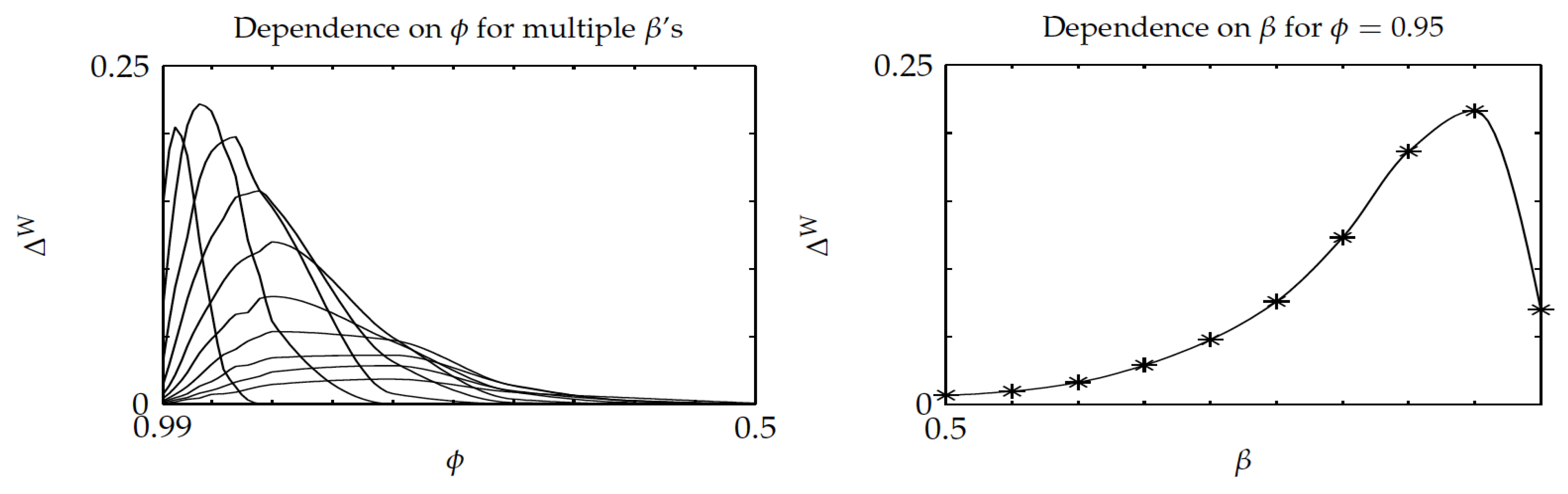
Figure 5 displays, in its left pane, the relative gap Δ W versus ϕ —note the inverted ϕ -axis used throughout—for multiple β , while using cubic interpolation. The gap starts at 0 as ϕ approaches 1 (as the optimal policy is then obtained), and then grows up to a maximum, which is below 0.18 % , and then decreases to 0 as ϕ gets smaller. That pattern agrees with intuition: for small enough ϕ , both the optimal and Whittle index policies initially pick a project and stick to it. Because the best such project can be determined by single-project evaluations, the Whittle index policy will correctly choose it. The right pane shows that Δ W is not monotonic in β , as it is increasing for small β and then decreases for β closer to 1. Hence, in the left pane, the higher peaks typically correspond to larger values of β .
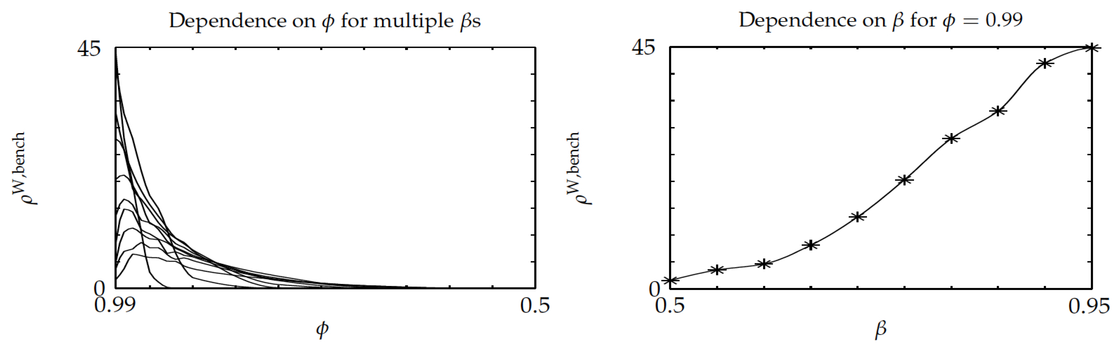
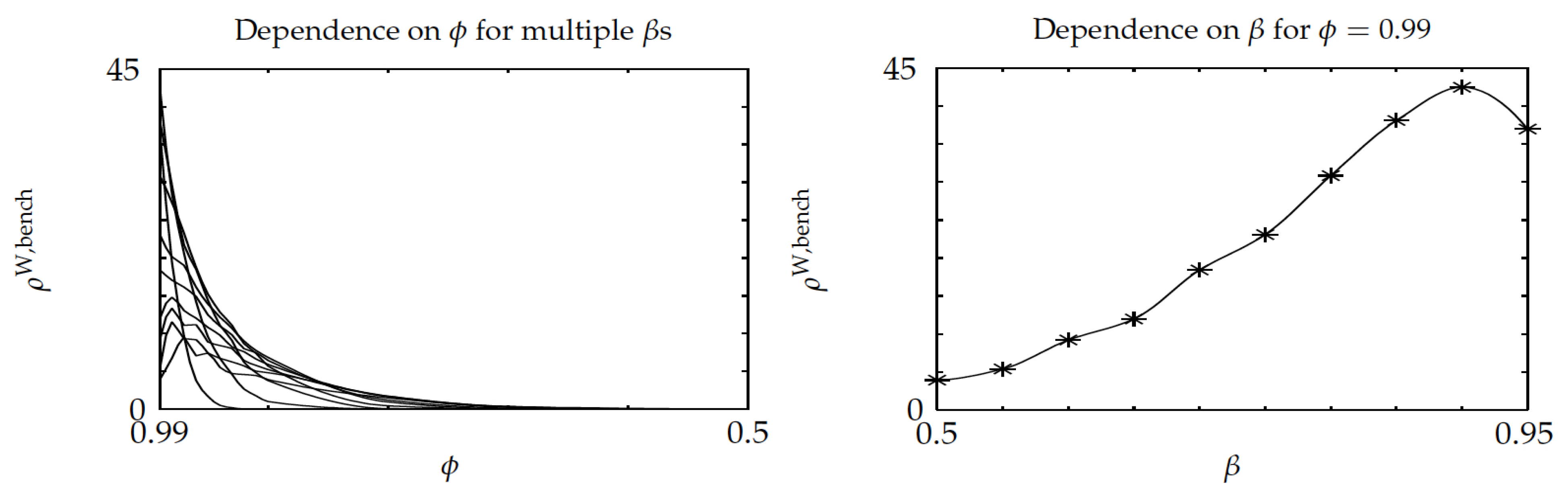
Figure 6 shows similar plots for the optimality-gap ratio ρ W , bench of the Whittle index over the benchmark policy. They highlight that the average optimality gap for the Whittle index policy remains below 45 % of that for the benchmark policy. The left pane shows that the ratio vanishes for ϕ that is small enough, as the Whittle index policy is then optimal. Additionally, the right pane shows that the ratio is increasing with β . Thus, in the left pane, for fixed ϕ , higher values correspond to larger β .
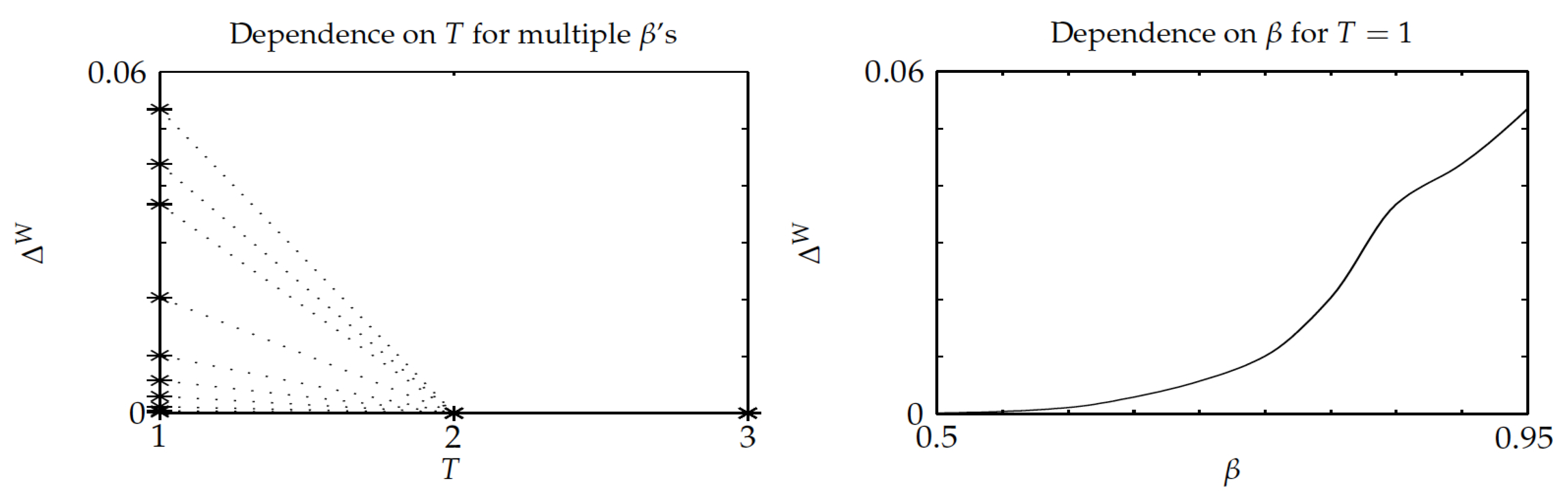
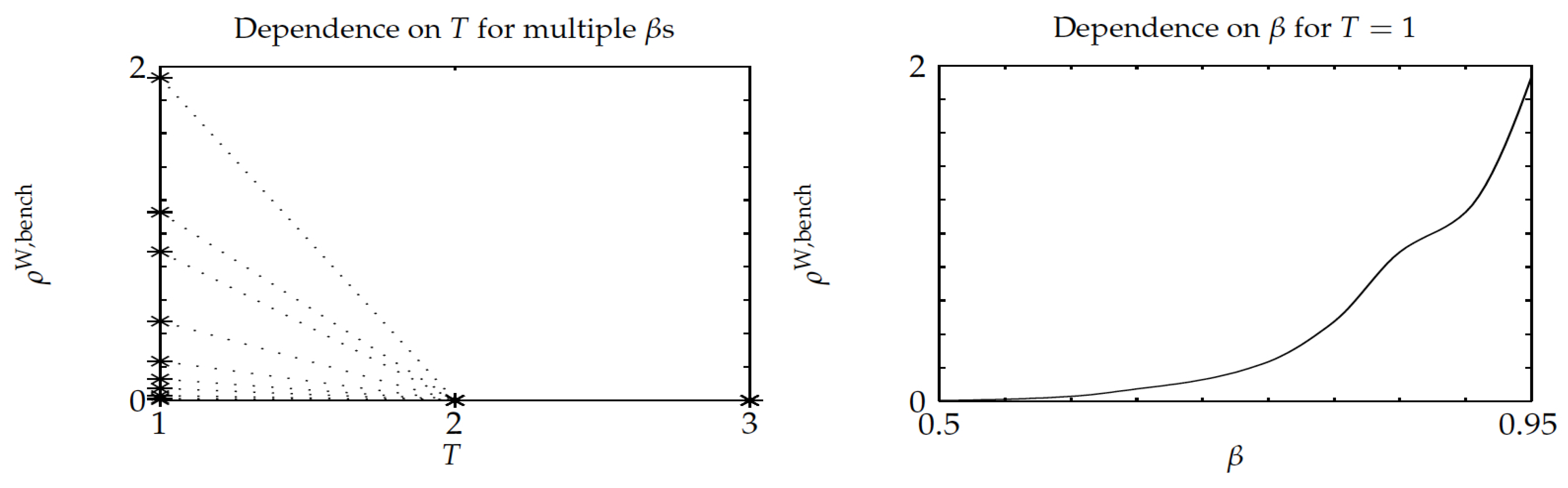
The third experiment was similar in nature as the previous one, but, when considering instead a constant setup delay T for each project, ϕ = β T . Figure 7 and Figure 8 show the results, which highlight that Whittle’s index policy was optimal for T 2 , its relative optimality gap did not exceed 0.06 % , and it substantially outperformed the benchmark Gittins-index policy, as the optimality-gap ratio stays below 2 % .
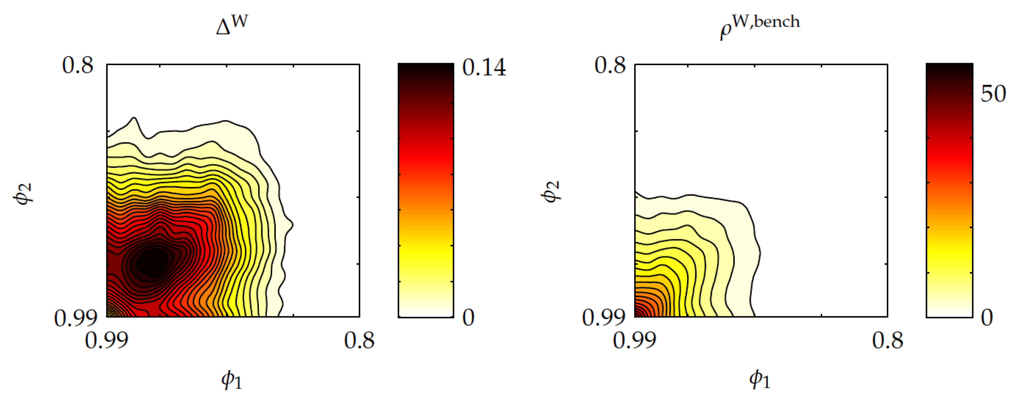
The fourth experiment addressed the effect of asymmetric (and constant) setup delay transforms, with these varying over the range ( ϕ 1 , ϕ 2 ) [ 0.8 , 0.99 ] 2 , in two-project instances with discount factor β = 0.9 . In the left contour plot in Figure 9 it is shown that the average relative optimality gap of Whittle’s index policy, Δ W , reaches a maximum of approximately 0.14 % , and it vanishes as both ϕ 1 and ϕ 2 get close to unity, and as either of them becomes small enough. The right contour plot shows that the optimality-gap ratio ρ W reaches the maximum values of nearly 50 % , then vanishing as either ϕ 1 or ϕ 2 becomes sufficiently small.
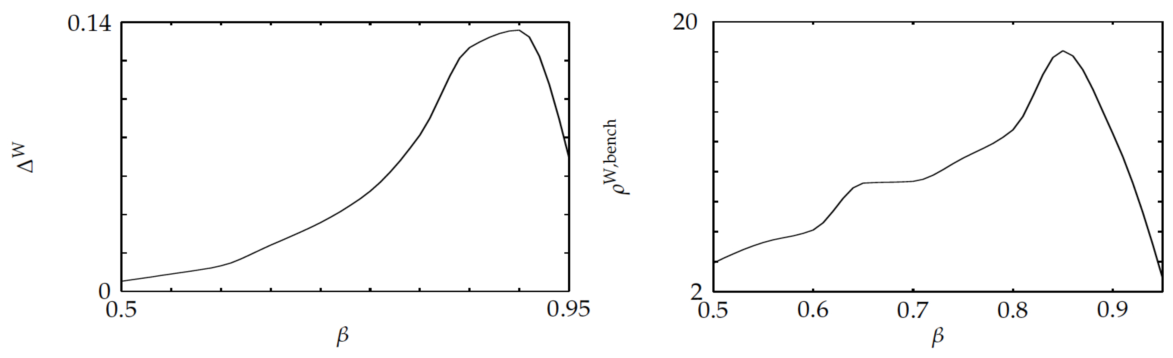
The fifth experiment studied the effect of state-dependent setup delay parameters ϕ i , as the discount factor is changed. Uniform[0.9, 1] i.i.d. state-dependent setup costs were randomly generated for every instance. The left pane shown in Figure 10 displays the average relative optimality gap versus the discount factor, showing that such a gap stays below 0.14 % . The right pane highlights that the average optimality-gap ratio ρ W , bench stays below 20 % .
The sixth experiment considered the relative performance of Whittle’s index policy on three-project instances in terms of a setup delay parameter ϕ and discount factor, while using a random sample of 100 instances of three eight-state projects. For each instance, the parameters varied over the range ( ϕ , β ) [ 0.5 , 0.99 ] × [ 0.5 , 0.95 ] . The results are displayed in Figure 11 and Figure 12, which are the counterparts of Figure 5 and Figure 6. Comparing Figure 5 and Figure 11 shows a slight degradation of performance for Whittle’s index policy in the latter, although the average gap Δ W stays small, beneath 0.25 % . Comparing Figure 6 and Figure 12 shows similar values for the ratio ρ W , bench .

8. Conclusions

Bandit models with switching penalties are relevant for a wide variety of applications. Computing optimal policies is generally intractable, which motivates the search for simple policies that can be implemented in practice and perform well. Index policies are an appealing class of policies, which have been proposed for such problems. Yet, while algorithms are given in [10,27] for computing the Asawa and Teneketzis index for a bandit with switching costs only, no algorithms have been given in the literature in order to compute the extension of such an index for bandits with switching penalties that incorporate switching delays. This paper presents the first such algorithm. It further provides evidence in a numerical study that the resulting index policy is nearly optimal across the instances considered. This work could be extended in several directions, including developing specialized algorithms for computing the index, in particular, models that arise in applications.

Funding

This research has been developed over a number of years, and has been funded in part by the Spanish Government under grants MEC MTM2004-02334 and MTM2007-63140, and PID2019-109196GB-I00 / AEI / 10.13039/501100011033. This work has also been funded in part by the Comunidad de Madrid in the setting of the multi-year agreement with Universidad Carlos III de Madrid within the line of activity “Excelencia para el Profesorado Universitario”, in the framework of the V Regional Plan of Scientific Research and Technological Innovation 2016–2020.

Institutional Review Board Statement

Not applicable.

Informed Consent Statement

Not applicable.

Data Availability Statement

The data presented in this study are available on request from the corresponding author. The data have not been made publicly available because the article describes in full detail how they can be generated by computer simulation and computational experiments.

Acknowledgments

The author has presented a preliminary version of this work at ValueTools ’07, the Second International Conference on Performance Evaluation Methodologies and Tools, which appears in abridged form in the online proceedings [51]. A preliminary version was also posted as the working paper [52].

Conflicts of Interest

The author declares no conflict of interest.

References

  1. Gittins, J.C. Multi-Armed Bandit Allocation Indices; Wiley: Chichester, UK, 1989. [Google Scholar]
  2. Gittins, J.C.; Jones, D.M. A dynamic allocation index for the sequential design of experiments. In Progress in Statistics (Eur. Meeting of Statisticians, Budapest, 1972); Gani, J., Sarkadi, K., Vincze, I., Eds.; North-Holland: Amsterdam, The Netherlands, 1974; pp. 241–266. [Google Scholar]
  3. Gittins, J.C. Bandit processes and dynamic allocation indices. J. R. Statist. Soc. Ser. B 1979, 41, 148–177. [Google Scholar] [CrossRef] [Green Version]
  4. Whittle, P. Multi-armed bandits and the Gittins index. J. R. Statist. Soc. Ser. B 1980, 42, 143–149. [Google Scholar] [CrossRef]
  5. Weber, R. On the Gittins index for multiarmed bandits. Ann. Appl. Probab. 1992, 2, 1024–1033. [Google Scholar] [CrossRef]
  6. Bertsimas, D.; Niño-Mora, J. Conservation laws, extended polymatroids and multiarmed bandit problems; a polyhedral approach to indexable systems. Math. Oper. Res. 1996, 21, 257–306. [Google Scholar] [CrossRef]
  7. Bellman, R. A problem in the sequential design of experiments. Sankhyā 1956, 16, 221–229. [Google Scholar]
  8. Varaiya, P.P.; Walrand, J.C.; Buyukkoc, C. Extensions of the multiarmed bandit problem: The discounted case. IEEE Trans. Automat. Control 1985, 30, 426–439. [Google Scholar] [CrossRef]
  9. Banks, J.S.; Sundaram, R.K. Switching costs and the Gittins index. Econometrica 1994, 62, 687–694. [Google Scholar] [CrossRef]
  10. Asawa, M.; Teneketzis, D. Multi-armed bandits with switching penalties. IEEE Trans. Automat. Control 1996, 41, 328–348. [Google Scholar] [CrossRef]
  11. Jun, T.S. Survey on the bandit problem with switching costs. De Econ. 2004, 152, 513–541. [Google Scholar] [CrossRef]
  12. Agrawal, R.; Hegde, M.V.; Teneketzis, D. Asymptotically efficient adaptive allocation rules for the multiarmed bandit problem with switching cost. IEEE Trans. Automat. Control 1988, 33, 899–906. [Google Scholar] [CrossRef] [Green Version]
  13. Van Oyen, M.P.; Pandelis, D.G.; Teneketzis, D. Optimality of index policies for stochastic scheduling with switching penalties. J. Appl. Probab. 1992, 29, 957–966. [Google Scholar] [CrossRef] [Green Version]
  14. Bergemann, D.; Valimaki, J. Stationary multi-choice bandit problems. J. Econ. Dyn. Control 2001, 25, 1585–1594. [Google Scholar] [CrossRef] [Green Version]
  15. Sundaram, R.K. Generalized bandit problems. In Social Choice and Strategic Decisions; Austen-Smith, D., Duggan, J., Eds.; Studies in Choice and Welfare; Springer: Berlin, Germany, 2005; pp. 131–162. [Google Scholar]
  16. Arlotto, A.; Chick, S.E.; Gans, N. Optimal hiring and retention policies for heterogeneous workers who learn. Manag. Sci. 2014, 60, 110–129. [Google Scholar] [CrossRef] [Green Version]
  17. Hauser, J.R.; Liberali, G.; Urban, G. Website morphing 2.0: Switching costs, partial exposure, random exit, and when to morph. Manag. Sci. 2014, 60, 1594–1616. [Google Scholar] [CrossRef]
  18. Liberali, G.B.; Hauser, J.R.; Urban, G.L. Morphing theory and application. In Handbook of Marketing Decision Models; Wierenga, B., van der Lans, R., Eds.; International Series in Operations Research & Management Science; Springer: Cham, Switzerland, 2017; Chapter 18; Volume 254, pp. 531–562. [Google Scholar]
  19. Lin, S.; Zhang, J.J.; Hauser, J.R. Learning from experience, simply. Mark. Sci. 2015, 34, 1–19. [Google Scholar] [CrossRef]
  20. Huang, J.; Gan, X.; Feng, X. Multi-armed bandit based opportunistic channel access: A consideration of switch cost. In Proceedings of the IEEE International Conference on Communications—Ad-hoc and Sensor Networking Symposium, Budapest, Hungary, 9–13 June 2013; pp. 1651–1655. [Google Scholar]
  21. Qin, Z.Q.; Wang, J.L.; Chen, J.; Sun, Y.M.; Du, Z.Y.; Xu, Y.H. Opportunistic channel access with repetition time diversity and switching cost: A block multi-armed bandit approach. Wirel. Netw. 2018, 24, 1683–16977. [Google Scholar] [CrossRef]
  22. McCardle, K.F.; Tsetlin, I.; Winkler, R.L. When to abandon a research project and search for a new one. Oper. Res. 2018, 66, 799–813. [Google Scholar] [CrossRef]
  23. Savelov, M.P. Gittins index for simple family of Markov bandit processes with switching cost and no discounting. Theory Probab. Appl. 2019, 64, 355–364. [Google Scholar] [CrossRef]
  24. Dusonchet, F.; Hongler, M.O. Optimal hysteresis for a class of deterministic deteriorating two-armed bandit problem with switching costs. Automatica 2003, 39, 1947–1955. [Google Scholar] [CrossRef]
  25. Dusonchet, F.; Hongler, M.O. Priority index heuristic for multi-armed bandit problems with set-up costs and/or set-up time delays. Int. J. Comput. Integr. Manuf. 2006, 19, 210–219. [Google Scholar] [CrossRef]
  26. Mason, A.J.; Anderson, E.J. Minimizing flow time on a single machine with job classes and setup times. Nav. Res. Logist. 1991, 64, 333–350. [Google Scholar] [CrossRef]
  27. Niño-Mora, J. A faster index algorithm and a computational study for bandits with switching costs. INFORMS J. Comput. 2008, 20, 255–269. [Google Scholar] [CrossRef]
  28. Niño-Mora, J. A (2/3)n3 fast-pivoting algorithm for the Gittins index and optimal stopping of a Markov chain. INFORMS J. Comput. 2007, 19, 596–606. [Google Scholar] [CrossRef] [Green Version]
  29. Whittle, P. Restless bandits: Activity allocation in a changing world. J. Appl. Probab. 1988, 25A, 287–298. [Google Scholar] [CrossRef]
  30. Niño-Mora, J. Restless bandits, partial conservation laws and indexability. Adv. Appl. Probab. 2001, 33, 76–98. [Google Scholar] [CrossRef] [Green Version]
  31. Niño-Mora, J. Dynamic allocation indices for restless projects and queueing admission control: A polyhedral approach. Math. Program. 2002, 93, 361–413. [Google Scholar] [CrossRef]
  32. Niño-Mora, J. Restless bandit marginal productivity indices, diminishing returns and optimal control of make-to-order/make-to-stock M/G/1 queues. Math. Oper. Res. 2006, 31, 50–84. [Google Scholar] [CrossRef]
  33. Niño-Mora, J. A verification theorem for threshold-indexability of real-state discounted restless bandits. Math. Oper. Res. 2020, 45, 465–496. [Google Scholar] [CrossRef]
  34. Niño-Mora, J. Dynamic priority allocation via restless bandit marginal productivity indices. Top 2007, 15, 161–198. [Google Scholar] [CrossRef]
  35. Papadimitriou, C.H.; Tsitsiklis, J.N. The complexity of optimal queuing network control. Math. Oper. Res. 1999, 24, 293–305. [Google Scholar] [CrossRef] [Green Version]
  36. Qian, Y.; Zhang, C.; Krishnamachari, B.; Tambe, M. Restless poachers: Handling exploration-exploitation tradeoffs in security domains. In Proceedings of the 2016 International Conference on Autonomous Agents & Multiagent Systems, Singapore, 9–13 May 2016; ACM: New York, NY, USA, 2016; pp. 123–131. [Google Scholar]
  37. Fu, J.; Moran, B.; Guo, J.; Wong, E.W.M.; Zukerman, M. Asymptotically optimal job assignment for energy-efficient processor-sharing server farms. IEEE J. Sel. Areas Commun. 2016, 34, 4008–4023. [Google Scholar] [CrossRef]
  38. Borkar, V.S.; Pattathil, S. Whittle indexability in egalitarian processor sharing systems. Ann. Oper. Res. 2017, 1–21. [Google Scholar] [CrossRef] [Green Version]
  39. Borkar, V.S.; Ravikumar, K.; Saboo, K. An index policy for dynamic pricing in cloud computing under price commitments. Appl. Math. 2017, 44, 215–245. [Google Scholar] [CrossRef]
  40. Borkar, V.S.; Kasbekar, G.S.; Pattathil, S.; Shetty, P.Y. Opportunistic scheduling as restless bandits. IEEE Trans. Control Netw. Syst. 2018, 5, 1952–1961. [Google Scholar] [CrossRef] [Green Version]
  41. Gerum, P.C.L.; Altay, A.; Baykal-Gursoy, M. Data-driven predictive maintenance scheduling policies for railways. Transport. Res. Part C Emerg. Technol. 2019, 107, 137–154. [Google Scholar] [CrossRef]
  42. Abbou, A.; Makis, V. Group maintenance: A restless bandits approach. INFORMS J. Comput. 2019, 31, 719–731. [Google Scholar] [CrossRef]
  43. Ayer, T.; Zhang, C.; Bonifonte, A.; Spaulding, A.C.; Chhatwal, J. Prioritizing hepatitis C treatment in US prisons. Oper. Res. 2019, 67, 853–873. [Google Scholar] [CrossRef] [Green Version]
  44. Niño-Mora, J. Resource allocation and routing in parallel multi-server queues with abandonments for cloud profit maximization. Comput. Oper. Res. 2019, 103, 221–236. [Google Scholar] [CrossRef]
  45. Fu, J.; Moran, B. Energy-efficient job-assignment policy with asymptotically guaranteed performance deviation. IEEE/ACM Trans. Netw. 2020, 28, 1325–1338. [Google Scholar] [CrossRef] [Green Version]
  46. Hsu, Y.P.; Modiano, E.; Duan, L.J. Scheduling algorithms for minimizing age of information in wireless broadcast networks with random arrivals. IEEE Trans. Mob. Comput. 2020, 19, 2903–2915. [Google Scholar] [CrossRef]
  47. Sun, J.Z.; Jiang, Z.Y.; Krishnamachari, B.; Zhou, S.; Niu, Z.S. Closed-form Whittle’s index-enabled random access for timely status update. IEEE Trans. Commun. 2020, 68, 1538–1551. [Google Scholar] [CrossRef]
  48. Li, D.; Ding, L.; Connor, S. When to switch? Index policies for resource scheduling in emergency response. Prod. Oper. Manag. 2020, 29, 241–262. [Google Scholar] [CrossRef]
  49. Niño-Mora, J. A fast-pivoting algorithm for Whittle’s restless bandit index. Mathematics 2020, 8, 2226. [Google Scholar] [CrossRef]
  50. Yao, D.D. Comments on: “Dynamic priority allocation via restless bandit marginal productivity indices” [Top 15 (2007), no. 2, 161–198] by J. Niño-Mora. Top 2007, 15, 220–223. [Google Scholar] [CrossRef]
  51. Niño-Mora, J. Computing an index policy for bandits with switching penalties. In Proceedings of the ValueTools ’07, the Second International Conference on Performance Evaluation Methodologies and Tools, Nantes, France, 23–25 October 2007; ICST: Brussels, Belgium, 2007. Available online: https://dl.acm.org/doi/10.5555/1345263.1345361 (accessed on 29 December 2020).
  52. Niño-Mora, J. Two-Stage Index Computation for Bandits with Switching Penalties II: Switching Delays; Working Paper 07-42, Statistics and Econometrics Series 10; Univ. Carlos III de Madrid: Madrid, Spain, 2007. [Google Scholar]
Figure 1. Illustration for the proof of Theorem 1.
Mathematics 09 00052 g001
Figure 2. Switching index versus setup delay transform.
Mathematics 09 00052 g002
Figure 3. Continuation and switching indices versus setdown delay transform.
Mathematics 09 00052 g003
Figure 4. Exp. 1: Runtimes of index algorithms.
Mathematics 09 00052 g004
Figure 5. Exp. 2: Average optimality gap (%) of Whittle’s index policy.
Mathematics 09 00052 g005
Figure 6. Exp. 2: Average optimality-gap ratio (%) of Whittle’s index policy over the benchmark policy.
Mathematics 09 00052 g006
Figure 7. Exp. 3: Average optimality gap (%) of Whittle’s index policy.
Mathematics 09 00052 g007
Figure 8. Exp. 3: Average optimality-gap ratio (%) of Whittle’s index over benchmark policy.
Mathematics 09 00052 g008
Figure 9. Exp. 4: Average relative performance (%) of Whittle’s index policy versus ( ϕ 1 , ϕ 2 ) , for β = 0.9 .
Mathematics 09 00052 g009
Figure 10. Exp. 5: Average relative performance (%) of Whittle’s index policy with state-dependent setup delays.
Mathematics 09 00052 g010
Figure 11. Exp. 6: Version of Figure 5 for three-project instances.
Mathematics 09 00052 g011
Figure 12. Exp. 6: Version of Figure 6 for three-project instances.
Mathematics 09 00052 g012
Table 1. Some notation employed in the paper.
M { 1 , , M } set of projects
t k decision periods
X m ( t ) , X ( t ) project state in period t
X m , X project state space
A m ( t ) , A ( t ) action chosen on a project in period t
A m ( t ) , A ( t ) previously chosen action
R m ( i m ) , R ( i ) rewards
β one-period discount factor
p m ( i m , j m ) , p ( i , j ) state-transition probabilities
c m ( i m ) , c ( i ) setup costs
d m ( i m ) , d ( i ) setdown costs
ξ m ( i m ) , ξ ( i ) setup delays
ϕ m ( i m ) , ϕ ( i ) setup delay z-transforms, for z = β
ψ m , ψ setdown delay z-transform, for z = β
Y m ( t ) , Y ( t ) augmented state in period t
Y m , Y augmented state space
F i π , F y π , F π reward metric
G i π , G y π , G π resource consumption metric
f i π , f y π marginal reward metric
g i π , g y π marginal resource consumption metric
λ i S , λ y S marginal productivity metric
Publisher’s Note: MDPI stays neutral with regard to jurisdictional claims in published maps and institutional affiliations.

