HTLV/HIV Dual Infection: Modeling and Analysis

Abstract

Human T-lymphotropic virus type I (HTLV-I) and human immunodeficiency virus (HIV) are two famous retroviruses that share similarities in their genomic organization, and differ in their life cycle as well. It is known that HTLV-I and HIV have in common a way of transmission via direct contact with certain body fluids related to infected patients. Thus, it is not surprising that a single-infected person with one of these viruses can be dually infected with the other virus. In the literature, many researchers have devoted significant efforts for modeling and analysis of HTLV or HIV single infection. However, the dynamics of HTLV/HIV dual infection has not been formulated. In the present paper, we formulate an HTLV/HIV dual infection model. The model includes the impact of the Cytotoxic T lymphocyte (CTLs) immune response, which is important to control the dual infection. The model describes the interaction between uninfected CD$4^{+}$T cells, HIV-infected cells, HTLV-infected cells, free HIV particles, HIV-specific CTLs, and HTLV-specific CTLs. We establish that the solutions of the model are non-negative and bounded. We calculate all steady states of the model and deduce the threshold parameters which determine the existence and stability of the steady states. We prove the global asymptotic stability of all steady states by utilizing the Lyapunov function and Lyapunov–LaSalle asymptotic stability theorem. We solve the system numerically to illustrate the our main results. In addition, we compared between the dynamics of single and dual infections.

1. Introduction

Human immunodeficiency virus (HIV) infects the human body and causes acquired immunodeficiency syndrome (AIDS), which is one of the deadly diseases. HIV is a retrovirus that infects the uninfected CD$4^{+}$T cells, which play an important role in the immune system. Cytotoxic T lymphocytes (CTLs) and antibodies are the two arms of the immune system. HIV-specific CTLs kill the HIV-infected cells. On the other side, B cells generate HIV-specific antibodies to neutralize viruses circulating in the plasma. Therefore, the infection can relatively be controlled for a long period up to 10 or even 15 years [1]. During this long period, the concentration of uninfected CD$4^{+}$T cells in the blood are decaying. The concentration of CD$4^{+}$T cells in an uninfected individual is 1000 cells/mm${}^3$. The individual is called an AIDS patient if the concentration of CD$4^{+}$T cells goes below 200 cells/mm${}^3$. During the last few decades, mathematical modeling of HIV infections have witnessed a significant development [2,3,4,5,6,7]. Stability analysis has also become one of the very important and helpful methods for better understanding the within-host HIV dynamics (see e.g., [8,9,10,11,12,13,14,15,16,17]).

Nowak and Bangham [3] have formulated the basic HIV infection model which describes the interaction between uninfected CD$4^{+}$T cells, HIV-infected CD$4^{+}$T cells, and free HIV particles as:

$$\left\{\begin{array}{c}\frac{dS}{dt}=\rho -\alpha S-{\eta }_{1}SV,\hfill \\ \frac{dI}{dt}={\eta }_{1}SV-aI,\hfill \\ \frac{dV}{dt}=bI-\epsilon V,\hfill \end{array}\right.$$

(1)

where $S=S\left(t\right),$ $I=I\left(t\right)$, and $V=V\left(t\right)$ are the concentrations of uninfected CD$4^{+}$T cells, HIV-infected cells, and free HIV particles at time t, respectively. The HIV virions can replicate using free-to-cell transmission. The uninfected CD$4^{+}$T cells are produced at specific constant rate $\rho$. The term ${\eta }_{1}SV$ refers to the rate at which new infections appear by free-to-cell contact between free HIV particles and uninfected CD$4^{+}$T cells. The term $bI$ refers to the rate at which free HIV particles are generated. The natural death rates of the uninfected CD$4^{+}$T cells, HIV-infected cells, and free HIV particles are given by $\alpha S$, $aI$, and $\epsilon V$, respectively. To incorporate the effect of the CTL immune response, Nowak and Bangham [3] have presented the following model:

$$\left\{\begin{array}{c}\frac{dS}{dt}=\rho -\alpha S-{\eta }_{1}SV,\hfill \\ \frac{dI}{dt}={\eta }_{1}SV-aI-{\mu }_1{C}^{I}I,\hfill \\ \frac{dV}{dt}=bI-\epsilon V,\hfill \\ \frac{d{C}^I}{dt}={\sigma }_1{C}^{I}I-{\pi }_1{C}^I,\hfill \end{array}\right.$$

(2)

where $C^I=C^I\left(t\right)$ is the concentration of HIV-specific CTLs at time t. The term ${\mu }_1{C}^{I}I$ is the killing rate of active HIV-infected cells due to their specific immunity. The expansion rate of effective HIV-specific CTLs is given by ${\sigma }_1{C}^{I}I$. The term ${\pi }_1{C}^I$ represents the death rate of effective HIV-specific CTLs.

Human T-lymphotropic virus type I (HTLV-I) is an exogenous retrovirus that infects the human body and can lead to two diseases, one of them an inflammatory of the central nervous system known as HTLV-I-associated myelopathy/tropical spastic paraparesis (HAM/TSP) and the other an adult T-cell leukemia (ATL). The discovery of the first human retrovirus HTLV-I is back to 1980, and, after three years, the HIV was determined [18]. The infection is endemic in the Caribbean, southern Japan, the Middle East, South America, parts of Africa, Melanesia, and Papua New Guinea [19]. HTLV-I is a provirus that targets the uninfected CD$4^{+}$T cells. HTLV-I can spread to uninfected CD$4^{+}$T cells from infected-to-cell through the virological synapse [20]. During the primary infection stage of HTLV-I, the proviral load can reach high level, approximately 30–50% [21]. For HTLV-I carriers, about 2–5% percent develop symptoms of ATL and another 0.25–3% develop HAM/TSP [22]. Many researchers have shown concern towards studying the dynamical behavior and analysis of the HTLV-I single infection models which have been addressed in several works [23,24,25,26,27,28]. It has been reported in [29] that the CTLs play an effective part in limiting HTLV-I replication. They can identify and kill the Tax-expressing HTLV-infected CD$4^{+}$T cells. The within-host HTLV-I dynamics model with CTL immune response is given as follows [2]:

$$\left\{\begin{array}{c}\frac{dS}{dt}=\rho -\alpha S-{\eta }_{2}SY,\hfill \\ \frac{dY}{dt}=\phi {\eta }_{2}SY-\delta Y-{\mu }_2{C}^{Y}Y,\hfill \\ \frac{d{C}^Y}{dt}={\sigma }_2{C}^{Y}Y-{\pi }_2{C}^Y,\hfill \end{array}\right.$$

(3)

where $Y=Y\left(t\right)$ and $C^Y=C^Y\left(t\right)$ being the concentrations of HTLV-infected cells and HTLV-specific CTLs at time t, respectively. In contrast with HIV, the transmission of HTLV-I can only be from infected-to-cell, that is, the HTLV virions can survive only inside the host CD$4^{+}$T cells and cannot be detectable in the plasma. The uninfected CD$4^{+}$T cells become HTLV-infected cells due to infected-to-cell contact at rate ${\eta }_{2}SY$. The parameter $\phi \in (0,1)$ is a fraction represents the newly infected CD$4^{+}$T cells after surviving the immune response. The HTLV-infected cells are killed by their specific CTLs at rate ${\mu }_2{C}^{Y}Y$. The term ${\sigma }_2{C}^{Y}Y$ represents the expansion rate of HTLV-specific CTLs. The terms $\delta Y$ and ${\pi }_2{C}^Y$ denote the death rates of the HTLV-infected cells and HTLV-specific CTLs, respectively. This model has been developed and extended in several works which discussed the dynamical behavior of HTLV-I infection models, and how CTL immunity contributes to limiting the HTLV-I duplication in vivo (see [2,19,30,31,32,33,34,35,36,37,38]).

It has been discovered that the simultaneous infection by the two viruses affects the pathogenic development and influences the outcomes for associated chronic diseases [39]. In fact, concurrent infections with HTLV-I and HIV have occurred frequently in areas where people living at high risk activities such as needle injection sharing and unprotected sexual relationships. In addition, HTLV/HIV dual infections have documented in specific geographic regions where both retroviruses become endemic [40], and among those who belonged to a specific ethnic as well. For instance, the dual infection rates in peoples living in some parts of Brazil have reached 16% of HIV-infected patients [41]. In a recent work, it has been estimated that the HIV single infected patients have more exposure to be dual infected with HTLV-I at a higher rate initiating from 100 to 500 times in comparison with the uninfected peoples [42]. Moreover, some seroepidemiologic studies have reported that HTLV-infected patients are at risk to have a concurrent infection with HIV, and vice versa compared to those who are infection-free from the general population [40]. HTLV-I and HIV mainly attack the CD$4^{+}$T cells and lead to immune dysfunction as well; however, they also conflict no doubt with respect to the etiology of their pathogenic and clinical outcomes [43]. HTLV-I and HIV dual infection appears to have an overlap on the course of associated clinical outcomes with both viruses [40]. Many researchers have reported that HIV infected individuals who are possibly dual infected with HTLV-I can potentially be associated with clinical progression with AIDS. In contrast, HIV can modify HTLV-I expression in dual infected patients which leads them to a higher risk of developing HTLV-I related diseases such as TSP/HAM and ATL [40,42].

While many efforts have been made to investigate mathematical modeling and analysis of both HTLV-I and HIV single infection, almost none have focused on the modeling of HTLV/HIV dual infection dynamics. The only exception is the work of Elaiw and AlShamrani [44], where they have proposed an HTLV/HIV dual infection. The model presented in [44] is 8-dimensional ODEs which incorporated the latently HIV-infected and HTLV-infected cells. The model contained 23 parameters, however, to estimate such a large number of parameters requires a large number of measurements (blood samples) which are very difficult to obtain. Therefore, the aim of the present paper is to formulate and analyze a more applicable HTLV/HIV dual infection model with a smaller number of parameters. We show that the model is well-posed by establishing that the solutions of the model are non-negative and bounded. We derive a set of threshold parameters which govern the existence and stability of the steady states of the model. Global stability of all steady states is proven by formulating Lyapunov functions and utilizing the Lyapunov–LaSalle asymptotic stability theorem. We perform some numerical simulations to illustrate the theoretical results. Our proposed model and its mathematical analysis will be needed to help clinicians on estimating the appropriate time to initiate treatment in dually infected patients. Since an individual can be infected with two or more viruses in the same time, our model may be helpful to study different dual infections such as Coronavirus/Influenza, HIV/HCV, HIV/HBV, and HIV/Malaria.

The rest of the paper is organized as follows: In Section 2, we propose an HTLV/HIV dual infection model. In Section 3, we prove the non-negativity and boundedness of solutions of the proposed model. Then, we study the existence of all possible steady states of the model which depend on eight threshold parameters in Section 4. Moreover, in Section 5, we investigate the global stability of the eight equilibria by constructing suitable Lyapunov functions. These results are illustrated by numerical simulations in Section 6. Finally, in Section 7, we present some discussions and brief conclusions.

2. HTLV/HIV Dual Infection Model Formulation

In this section, we introduce an HTLV/HIV dual infection dynamics model. The dynamics of HTLV/HIV dual infection is schematically shown in Figure 1.

Figure 1. The schematic diagram of the HTLV/HIV dual infection dynamics in vivo.

We propose the following model:

$$\left\{\begin{array}{c}\frac{dS}{dt}=\rho -\alpha S-{\eta }_{1}SV-{\eta }_{2}SY,\hfill \\ \frac{dI}{dt}={\eta }_{1}SV-aI-{\mu }_1{C}^{I}I,\hfill \\ \frac{dY}{dt}=\phi {\eta }_{2}SY-\delta Y-{\mu }_2{C}^{Y}Y,\hfill \\ \frac{dV}{dt}=bI-\epsilon V,\hfill \\ \frac{d{C}^I}{dt}={\sigma }_1{C}^{I}I-{\pi }_1{C}^I,\hfill \\ \frac{d{C}^Y}{dt}={\sigma }_2{C}^{Y}Y-{\pi }_2{C}^Y,\hfill \end{array}\right.$$

(4)

where $(S,I,Y,V,C^I,C^Y)=(S,I,Y,V,C^I,C^Y)\left(t\right)$. All variables and parameters have the same biological definition as given above.

3. Preliminaries

Lemma 1.

For model (4), there exist ${\Delta }_j>0$, $j=1,...,5$ such that

$$0\le S\left(t\right),I\left(t\right)\le {\Delta }_1,0\le Y\left(t\right)\le {\Delta }_2,0\le V\left(t\right)\le {\Delta }_3,0\le C^I\left(t\right)\le {\Delta }_4,0\le C^Y\left(t\right)\le {\Delta }_5.$$

Proof. 

We have

$$\begin{array}{cc}\hfill \frac{dS}{dt}& {\mid }_{S=0}=\rho >0,\frac{dI}{dt}{\mid }_{I=0}={\eta }_{1}SV\ge 0\mathrm{for}\mathrm{all}S,V\ge 0,\frac{dY}{dt}{\mid }_{Y=0}=0,\hfill \\ \hfill \frac{dV}{dt}& {\mid }_{V=0}=bI\ge 0\mathrm{for}\mathrm{all}I\ge 0,\frac{d{C}^I}{dt}{\mid }_{C^I=0}=0,\frac{d{C}^Y}{dt}{\mid }_{C^Y=0}=0.\hfill \end{array}$$

This confirms that $(S,I,Y,V,C^I,C^Y)\left(t\right)\in {\mathbb{R}}_{\ge 0}^6$ for all $t\ge 0$ when $(S,I,Y,V,C^I,C^Y)\left(0\right)$ $\in {\mathbb{R}}_{\ge 0}^6$. Let

$$\mathsf{\Psi }=S+I+\frac{1}{\phi }Y+\frac{a}{2b}V+\frac{{\mu }_1}{{\sigma }_1}{C}^I+\frac{{\mu }_2}{\phi {\sigma }_2}{C}^Y.$$

Then,

$$\begin{array}{cc}\hfill \frac{d\mathsf{\Psi }}{dt}& =\rho -\alpha S-\frac{a}{2}I-\frac{\delta }{\phi }Y-\frac{a\epsilon }{2b}V-\frac{{\mu }_1{\pi }_1}{{\sigma }_1}{C}^I-\frac{{\mu }_2{\pi }_2}{\phi {\sigma }_2}{C}^Y\hfill \\ \hfill & \le \rho -\varphi \left(S+I+\frac{1}{\phi }Y+\frac{a}{2b}V+\frac{{\mu }_1}{{\sigma }_1}{C}^I+\frac{{\mu }_2}{\phi {\sigma }_2}{C}^Y\right)=\rho -\varphi \mathsf{\Psi },\hfill \end{array}$$

where $\varphi =min\{\alpha ,\frac{a}{2},\delta ,\epsilon ,{\pi }_1,{\pi }_2\}$. It follows that $0\le \mathsf{\Psi }\left(t\right)\le {\Delta }_1$ if $\mathsf{\Psi }\left(0\right)\le {\Delta }_1$ for $t\ge 0,$ where ${\Delta }_1=\frac{\rho }{\varphi }.$ Since S, $I,$ $Y,$ $V,$ $C^I$, and $C^Y$ are all non-negative, then $0\le S\left(t\right),I\left(t\right)\le {\Delta }_1$, $0\le Y\left(t\right)\le {\Delta }_2$, $0\le V\left(t\right)\le {\Delta }_3$, $0\le C^I\left(t\right)\le {\Delta }_4$, $0\le C^Y\left(t\right)\le {\Delta }_5$ if $S\left(0\right)+I\left(0\right)+\frac{1}{\phi }Y\left(0\right)+\frac{a}{2b}V\left(0\right)+\frac{{\mu }_1}{{\sigma }_1}{C}^I\left(0\right)+\frac{{\mu }_2}{\phi {\sigma }_2}{C}^Y\left(0\right)\le {\Delta }_1$, where ${\Delta }_2=\phi {\Delta }_1$, ${\Delta }_3={\displaystyle \frac{2b{\Delta }_1}{a}}$, ${\Delta }_4={\displaystyle \frac{{\sigma }_1{\Delta }_1}{{\mu }_1}}$ and ${\Delta }_5={\displaystyle \frac{\phi {\sigma }_2{\Delta }_1}{{\mu }_2}}$. □

4. Steady States

Now, we calculate all possible steady states of system (4). The steady states of the system satisfy the following algebraic equations:

$$\begin{array}{cc}\hfill 0& =\rho -\alpha S-{\eta }_{1}SV-{\eta }_{2}SY,\hfill \end{array}$$

(5)

$$\begin{array}{cc}\hfill 0& ={\eta }_{1}SV-aI-{\mu }_1{C}^{I}I,\hfill \end{array}$$

(6)

$$\begin{array}{cc}\hfill 0& =\phi {\eta }_{2}SY-\delta Y-{\mu }_2{C}^{Y}Y,\hfill \end{array}$$

(7)

$$\begin{array}{cc}\hfill 0& =bI-\epsilon V,\hfill \end{array}$$

(8)

$$\begin{array}{cc}\hfill 0& =\left({\sigma }_{1}I-{\pi }_1\right)C^I,\hfill \end{array}$$

(9)

$$\begin{array}{cc}\hfill 0& =\left({\sigma }_{2}Y-{\pi }_2\right)C^Y.\hfill \end{array}$$

(10)

We find that system (4) has eight possible steady states:

(i) Infection-free steady state, Đ${}_0=(S_0,0,0,0,0,0)$, where $S_0=\rho /\alpha$. In this case, the body is free from HIV and HTLV.

(ii) Persistent HIV single infection steady state with an ineffective immune response, Đ${}_1=(S_1,I_1,0,V_1,0,0),$ where

$$S_1={\displaystyle \frac{a\epsilon }{{\eta }_{1}b}},I_1=\frac{\epsilon \alpha }{{\eta }_{1}b}\left(\frac{{\eta }_{1}b{S}_0}{a\epsilon }-1\right),V_1=\frac{\alpha }{{\eta }_1}\left(\frac{{\eta }_{1}b{S}_0}{a\epsilon }-1\right).$$

Therefore, Đ${}_1$ exists when

$$\frac{{\eta }_{1}b{S}_0}{a\epsilon }>1.$$

It is clear that at the steady state Đ${}_1$ the HIV single infection persists with an ineffective immune response. The basic HIV single infection reproduction number for system (4) is given by:

$${\Re }_1=\frac{{\eta }_{1}b{S}_0}{a\epsilon }.$$

The parameter ${\Re }_1$ decides whether or not a persistent HIV infection can be established. In terms of ${\Re }_1$, we can write

$$S_1={\displaystyle \frac{S_0}{{\Re }_1}},I_1=\frac{\epsilon \alpha }{{\eta }_{1}b}\left({\Re }_1-1\right),V_1=\frac{\alpha }{{\eta }_1}\left({\Re }_1-1\right).$$

(iii) Persistent HTLV single infection steady state with an ineffective immune response, Đ${}_2=(S_2,0,Y_2,0,0,0)$, where

$$S_2={\displaystyle \frac{\delta }{\phi {\eta }_2}},Y_2=\frac{\alpha }{{\eta }_2}\left(\frac{\phi {\eta }_2{S}_0}{\delta }-1\right).$$

Therefore, Đ${}_2$ exists when

$$\frac{\phi {\eta }_2{S}_0}{\delta }>1.$$

At the steady state Đ${}_2$, the chronic HTLV single infection persists with an ineffective immune response. The basic HTLV single infection reproduction number for system (4) is given as:

$${\Re }_2=\frac{\phi {\eta }_2{S}_0}{\delta }.$$

The parameter ${\Re }_2$ decides whether or not a persistent HTLV infection can be established. In terms of ${\Re }_2$, we can write

$$S_2={\displaystyle \frac{S_0}{{\Re }_2}},Y_2=\frac{\alpha }{{\eta }_2}\left({\Re }_2-1\right).$$

(iv) Persistent HIV single infection steady state with only effective HIV-specific CTL, Đ${}_3=(S_3,I_3,0,V_3,C_3^I,0)$, where

$$S_3={\displaystyle \frac{\epsilon {\sigma }_1\rho }{{\pi }_1{\eta }_{1}b+\alpha \epsilon {\sigma }_1}},I_3=\frac{{\pi }_1}{{\sigma }_1},V_3=\frac{b}{\epsilon }{I}_3=\frac{b{\pi }_1}{\epsilon {\sigma }_1},C_3^I={\displaystyle \frac{a}{{\mu }_1}}\left[{\displaystyle \frac{{\sigma }_1\rho {\eta }_{1}b}{a\left({\pi }_1{\eta }_{1}b+\alpha \epsilon {\sigma }_1\right)}}-1\right].$$

We note that Đ${}_3$ exists when ${\displaystyle \frac{{\sigma }_1\rho {\eta }_{1}b}{a\left({\pi }_1{\eta }_{1}b+\alpha \epsilon {\sigma }_1\right)}}>1$. We define the HIV-specific CTL reproduction number in case of HIV single infection as follows:

$${\Re }_3={\displaystyle \frac{{\sigma }_1\rho {\eta }_{1}b}{a\left({\pi }_1{\eta }_{1}b+\alpha \epsilon {\sigma }_1\right)}}.$$

Thus, $C_3^I={\displaystyle \frac{a}{{\mu }_1}}({\Re }_3-1)$. The parameter ${\Re }_3$ determines whether or not the HIV-specific CTL immune response is effective in the absence of HTLV.

(v) Persistent HTLV single infection steady state with only effective HTLV-specific CTL, Đ${}_4=(S_4,0,Y_4,0,0,C_4^Y)$, where

$$S_4={\displaystyle \frac{{\sigma }_2\rho }{{\pi }_2{\eta }_2+\alpha {\sigma }_2}},Y_4=\frac{{\pi }_2}{{\sigma }_2},C_4^Y={\displaystyle \frac{\delta }{{\mu }_2}}\left[{\displaystyle \frac{{\sigma }_2\rho \phi {\eta }_2}{\delta \left({\pi }_2{\eta }_2+\alpha {\sigma }_2\right)}}-1\right].$$

We note that Đ${}_4$ exists when ${\displaystyle \frac{{\sigma }_2\rho \phi {\eta }_2}{\delta \left({\pi }_2{\eta }_2+\alpha {\sigma }_2\right)}}>1$. The HTLV-specific CTL reproduction number in the case of HTLV single infection is stated as:

$${\Re }_4={\displaystyle \frac{{\sigma }_2\rho \phi {\eta }_2}{\delta \left({\pi }_2{\eta }_2+\alpha {\sigma }_2\right)}}.$$

Thus, $C_4^Y={\displaystyle \frac{\delta }{{\mu }_2}}({\Re }_4-1)$. The parameter ${\Re }_4$ determines whether or not the HTLV-specific CTL immune response is effective in the absence of HIV.

(vi) Persistent HTLV/HIV dual infection steady state with only effective HIV-specific CTL, Đ${}_5=(S_5,I_5,Y_5,V_5,C_5^I,0)$, where

$$\begin{array}{cc}\hfill S_5& ={\displaystyle \frac{\delta }{\phi {\eta }_2}}=S_2,I_5=\frac{{\pi }_1}{{\sigma }_1}=I_3,V_5=\frac{b{\pi }_1}{\epsilon {\sigma }_1}=V_3,\hfill \\ \hfill Y_5& ={\displaystyle \frac{{\pi }_1{\eta }_{1}b+\alpha \epsilon {\sigma }_1}{\epsilon {\eta }_2{\sigma }_1}}\left[\frac{\rho \phi \epsilon {\eta }_2{\sigma }_1}{\delta \left({\pi }_1{\eta }_{1}b+\alpha \epsilon {\sigma }_1\right)}-1\right],\hfill \\ \hfill C_5^I& ={\displaystyle \frac{a}{{\mu }_1}}\left(\frac{{\eta }_{1}b\delta }{a\epsilon \phi {\eta }_2}-1\right)={\displaystyle \frac{a}{{\mu }_1}}\left({\Re }_1/{\Re }_2-1\right).\hfill \end{array}$$

We note that Đ${}_5$ exists when ${\Re }_1/{\Re }_2>1$ and $\frac{\rho \phi \epsilon {\eta }_2{\sigma }_1}{\delta \left({\pi }_1{\eta }_{1}b+\alpha \epsilon {\sigma }_1\right)}>1$. The HTLV infection reproduction number in the presence of HIV infection is stated as:

$${\Re }_5=\frac{\rho \phi \epsilon {\eta }_2{\sigma }_1}{\delta \left({\pi }_1{\eta }_{1}b+\alpha \epsilon {\sigma }_1\right)}.$$

It is obvious that the parameter ${\Re }_5$ determines whether or not HIV-infected patients could be dually infected with HTLV. Thus, $Y_5={\displaystyle \frac{{\pi }_1{\eta }_{1}b+\alpha \epsilon {\sigma }_1}{\epsilon {\eta }_2{\sigma }_1}}\left({\Re }_5-1\right)$.

(vii) Persistent HTLV/HIV dual infection steady state with only effective HTLV-specific CTL, Đ${}_6=(S_6,I_6,Y_6,V_6,0,C_6^Y)$, where

$$\begin{array}{cc}\hfill S_6& ={\displaystyle \frac{a\epsilon }{{\eta }_{1}b}}=S_1,I_6={\displaystyle \frac{\epsilon \left({\pi }_2{\eta }_2+\alpha {\sigma }_2\right)}{b{\eta }_1{\sigma }_2}}\left[\frac{\rho b{\eta }_1{\sigma }_2}{a\epsilon \left({\pi }_2{\eta }_2+\alpha {\sigma }_2\right)}-1\right],Y_6=\frac{{\pi }_2}{{\sigma }_2}=Y_4,\hfill \\ \hfill V_6& ={\displaystyle \frac{{\pi }_2{\eta }_2+\alpha {\sigma }_2}{{\eta }_1{\sigma }_2}}\left[\frac{\rho b{\eta }_1{\sigma }_2}{a\epsilon \left({\pi }_2{\eta }_2+\alpha {\sigma }_2\right)}-1\right],C_6^Y={\displaystyle \frac{\delta }{{\mu }_2}}\left(\frac{a\epsilon \phi {\eta }_2}{{\eta }_{1}b\delta }-1\right)={\displaystyle \frac{\delta }{{\mu }_2}}\left({\Re }_2/{\Re }_1-1\right).\hfill \end{array}$$

We note that Đ${}_6$ exists when ${\Re }_2/{\Re }_1>1$ and $\frac{\rho b{\eta }_1{\sigma }_2}{a\epsilon \left({\pi }_2{\eta }_2+\alpha {\sigma }_2\right)}>1$. The HIV infection reproduction number in the presence of HTLV infection is stated as:

$${\Re }_6=\frac{\rho b{\eta }_1{\sigma }_2}{a\epsilon \left({\pi }_2{\eta }_2+\alpha {\sigma }_2\right)}.$$

Thus, $I_6={\displaystyle \frac{\epsilon \left({\pi }_2{\eta }_2+\alpha {\sigma }_2\right)}{b{\eta }_1{\sigma }_2}}\left({\Re }_6-1\right)$, $V_6={\displaystyle \frac{{\pi }_2{\eta }_2+\alpha {\sigma }_2}{{\eta }_1{\sigma }_2}}\left({\Re }_6-1\right)$. It is clear that the parameter ${\Re }_6$ determines whether or not HTLV-infected patients could be dually infected with HIV.

(viii) Persistent HTLV/HIV dual infection steady state with effective HIV-specific CTL and HTLV-specific CTL, Đ${}_7=(S_7,I_7,Y_7,V_7,C_7^I,C_7^Y)$, where

$$\begin{array}{cc}\hfill S_7& ={\displaystyle \frac{\epsilon {\sigma }_1{\sigma }_2\rho }{{\pi }_1{\eta }_{1}b{\sigma }_2+{\pi }_2{\eta }_2\epsilon {\sigma }_1+\alpha \epsilon {\sigma }_1{\sigma }_2}},\hfill \\ \hfill I_7& =\frac{{\pi }_1}{{\sigma }_1}=I_3=I_5,Y_7=\frac{{\pi }_2}{{\sigma }_2}=Y_4=Y_6,V_7=\frac{b{\pi }_1}{\epsilon {\sigma }_1}=V_3=V_5,\hfill \\ \hfill C_7^I& ={\displaystyle \frac{a}{{\mu }_1}}\left[{\displaystyle \frac{{\eta }_{1}b{\sigma }_1{\sigma }_2\rho }{a\left({\pi }_1{\eta }_{1}b{\sigma }_2+{\pi }_2{\eta }_2\epsilon {\sigma }_1+\alpha \epsilon {\sigma }_1{\sigma }_2\right)}}-1\right],\hfill \\ \hfill C_7^Y& ={\displaystyle \frac{\delta }{{\mu }_2}}\left[{\displaystyle \frac{\phi {\eta }_2\epsilon {\sigma }_1{\sigma }_2\rho }{\delta \left({\pi }_1{\eta }_{1}b{\sigma }_2+{\pi }_2{\eta }_2\epsilon {\sigma }_1+\alpha \epsilon {\sigma }_1{\sigma }_2\right)}}-1\right].\hfill \end{array}$$

It is obvious that Đ${}_7$ exists when ${\displaystyle \frac{{\eta }_{1}b{\sigma }_1{\sigma }_2\rho }{a\left({\pi }_1{\eta }_{1}b{\sigma }_2+{\pi }_2{\eta }_2\epsilon {\sigma }_1+\alpha \epsilon {\sigma }_1{\sigma }_2\right)}}>1$ and ${\displaystyle \frac{\phi {\eta }_2\epsilon {\sigma }_1{\sigma }_2\rho }{\delta \left({\pi }_1{\eta }_{1}b{\sigma }_2+{\pi }_2{\eta }_2\epsilon {\sigma }_1+\alpha \epsilon {\sigma }_1{\sigma }_2\right)}}>1$. Now, we define

$$\begin{array}{cc}\hfill {\Re }_7& ={\displaystyle \frac{{\eta }_{1}b{\sigma }_1{\sigma }_2\rho }{a\left({\pi }_1{\eta }_{1}b{\sigma }_2+{\pi }_2{\eta }_2\epsilon {\sigma }_1+\alpha \epsilon {\sigma }_1{\sigma }_2\right)}},\hfill \\ \hfill {\Re }_8& ={\displaystyle \frac{\phi {\eta }_2\epsilon {\sigma }_1{\sigma }_2\rho }{\delta \left({\pi }_1{\eta }_{1}b{\sigma }_2+{\pi }_2{\eta }_2\epsilon {\sigma }_1+\alpha \epsilon {\sigma }_1{\sigma }_2\right)}}.\hfill \end{array}$$

Clearly, Đ${}_7$ exists when ${\Re }_7>1$ and ${\Re }_8>1$ and we can write $C_7^I={\displaystyle \frac{a}{{\mu }_1}}\left({\Re }_7-1\right)$ and $C_7^Y={\displaystyle \frac{\delta }{{\mu }_2}}\left({\Re }_8-1\right).$ The parameter ${\Re }_7$ is the competed HIV-specific CTL reproduction number in case of HTLV/HIV dual infection. The parameter ${\Re }_8$ is the competed HTLV-specific CTL reproduction number in case of HTLV/HIV dual infection.

The eight threshold parameters are given as follows:

$$\begin{array}{cc}\hfill {\Re }_1& =\frac{{\eta }_{1}b{S}_0}{a\epsilon },{\Re }_2=\frac{\phi {\eta }_2{S}_0}{\delta },{\Re }_3={\displaystyle \frac{{\sigma }_1\rho {\eta }_{1}b}{a\left({\pi }_1{\eta }_{1}b+\alpha \epsilon {\sigma }_1\right)}},\hfill \\ \hfill {\Re }_4& ={\displaystyle \frac{{\sigma }_2\rho \phi {\eta }_2}{\delta \left({\pi }_2{\eta }_2+\alpha {\sigma }_2\right)}},{\Re }_5=\frac{\rho \phi \epsilon {\eta }_2{\sigma }_1}{\delta \left({\pi }_1{\eta }_{1}b+\alpha \epsilon {\sigma }_1\right)},{\Re }_6=\frac{\rho b{\eta }_1{\sigma }_2}{a\epsilon \left({\pi }_2{\eta }_2+\alpha {\sigma }_2\right)},\hfill \\ \hfill {\Re }_7& ={\displaystyle \frac{{\eta }_{1}b{\sigma }_1{\sigma }_2\rho }{a\left({\pi }_1{\eta }_{1}b{\sigma }_2+{\pi }_2{\eta }_2\epsilon {\sigma }_1+\alpha \epsilon {\sigma }_1{\sigma }_2\right)}},{\Re }_8={\displaystyle \frac{\phi {\eta }_2\epsilon {\sigma }_1{\sigma }_2\rho }{\delta \left({\pi }_1{\eta }_{1}b{\sigma }_2+{\pi }_2{\eta }_2\epsilon {\sigma }_1+\alpha \epsilon {\sigma }_1{\sigma }_2\right)}}.\hfill \end{array}$$

□

According to the above discussion, we sum up the existence conditions for all steady states in Table 1.

Table 1. Model (4) equilibria and their existence conditions.

Steady State	$\begin{array}{c}\mathbf{Definition}\hfill \end{array}$	Existence Conditions
Đ${}_0=(S_0,0,0,0,0,0)$	$\begin{array}{c}\mathrm{Infection}-\mathrm{free}\mathrm{steady}\mathrm{state}\hfill \end{array}$	None
Đ${}_1=(S_1,I_1,0,V_1,0,0)$	$\begin{array}{c}\mathrm{Persistent}\mathrm{HIV}\sin \mathrm{gle}\mathrm{infection}\mathrm{steady}\mathrm{state}\hfill \\ \mathrm{with}\mathrm{an}\mathrm{ineffective}\mathrm{immune}\mathrm{response}\hfill \end{array}$	${\Re }_1>1$
Đ${}_2=(S_2,0,Y_2,0,0,0)$	$\begin{array}{c}\mathrm{Persistent}\mathrm{HTLV}\sin \mathrm{gle}\mathrm{infection}\mathrm{steady}\mathrm{state}\hfill \\ \mathrm{with}\mathrm{an}\mathrm{ineffective}\mathrm{immune}\mathrm{response}\hfill \end{array}$	${\Re }_2>1$
Đ${}_3=(S_3,I_3,0,V_3,C_3^I,0)$	$\begin{array}{c}\mathrm{Persistent}\mathrm{HIV}\sin \mathrm{gle}\mathrm{infection}\mathrm{steady}\mathrm{state}\hfill \\ \mathrm{with}\mathrm{only}\mathrm{effective}\mathrm{HIV}-\mathrm{specific}\mathrm{CTL}\hfill \end{array}$	${\Re }_3>1$
Đ${}_4=(S_4,0,Y_4,0,0,C_4^Y)$	$\begin{array}{c}\mathrm{Persistent}\mathrm{HTLV}\sin \mathrm{gle}\mathrm{infection}\mathrm{steady}\mathrm{state}\hfill \\ \mathrm{with}\mathrm{only}\mathrm{effective}\mathrm{HTLV}-\mathrm{specific}\mathrm{CTL}\hfill \end{array}$	${\Re }_4>1$
Đ${}_5=(S_5,I_5,Y_5,V_5,C_5^I,0)$	$\begin{array}{c}\mathrm{Persistent}\mathrm{HTLV}/\mathrm{HIV}\mathrm{dual}\mathrm{infection}\mathrm{steady}\hfill \\ \mathrm{state}\mathrm{with}\mathrm{only}\mathrm{effective}\mathrm{HIV}-\mathrm{specific}\mathrm{CTL}\hfill \end{array}$	${\Re }_5>1$ and ${\Re }_1/{\Re }_2>1$
Đ${}_6=(S_6,I_6,Y_6,V_6,0,C_6^Y)$	$\begin{array}{c}\mathrm{Persistent}\mathrm{HTLV}/\mathrm{HIV}\mathrm{dual}\mathrm{infection}\mathrm{steady}\hfill \\ \mathrm{state}\mathrm{with}\mathrm{only}\mathrm{effective}\mathrm{HTLV}-\mathrm{specific}\mathrm{CTL}\hfill \end{array}$	${\Re }_6>1$ and ${\Re }_2/{\Re }_1>1$
Đ${}_7=(S_7,I_7,Y_7,V_7,C_7^I,C_7^Y)$	$\begin{array}{c}\mathrm{Persistent}\mathrm{HTLV}/\mathrm{HIV}\mathrm{dual}\mathrm{infection}\mathrm{steady}\hfill \\ \mathrm{state}\mathrm{with}\mathrm{effective}\mathrm{HIV}-\mathrm{specific}\mathrm{CTL}\mathrm{and}\hfill \\ \mathrm{HTLV}-\mathrm{specific}\mathrm{CTL}\hfill \end{array}$	${\Re }_7>1$ and ${\Re }_8>1$

5. Global Stability Analysis

In this section, we analyze the global asymptotic stability of all steady states by the Lyapunov method. For constructing Lyapunov functions, we follow the work of Korobeinikov [45].

To prove Theorems 1–8, we need the arithmetic-geometric mean inequality

$$\frac{1}{n}\sum _{i=1}^n{\chi }_i\ge \sqrt[n]{\prod _{i=1}^n{\chi }_i},{\chi }_i\ge 0,i=1,2,...$$

(11)

Let a function ${\mathsf{\Phi }}_j(S,I,Y,V,C^I,C^Y)$ and ${\mathsf{{\rm Y}}}_j^{{}^{\prime }}$ be the largest invariant subset of

$${\mathsf{{\rm Y}}}_j=\left\{(S,I,Y,V,C^I,C^Y):\frac{d{\mathsf{\Phi }}_j}{dt}=0\right\},j=0,1,2,...,7.$$

Theorem 1.

If ${\Re }_1\le 1$ and ${\Re }_2\le 1$, then Đ${}_0$ is globally asymptotically stable (G.A.S).

Proof. 

Define ${\mathsf{\Phi }}_0(S,I,Y,V,C^I,C^Y)$ as:

$${\mathsf{\Phi }}_0=S_0ϝ\left(\frac{S}{S_0}\right)+I+\frac{1}{\phi }Y+\frac{a}{b}V+\frac{{\mu }_1}{{\sigma }_1}{C}^I+\frac{{\mu }_2}{\phi {\sigma }_2}{C}^Y,$$

(12)

where

$$ϝ\left(\upsilon \right)=\upsilon -1-ln\upsilon .$$

Clearly, ${\mathsf{\Phi }}_0(S,I,Y,V,C^I,C^Y)>0$ for all $S,I,Y,V,C^I,C^Y>0,$ and ${\mathsf{\Phi }}_0(S_0,0,0,0,0,0)=0$. Calculating $\frac{d{\mathsf{\Phi }}_0}{dt}$ along the solutions of system (4) as:

$$\begin{array}{cc}\hfill \frac{d{\mathsf{\Phi }}_0}{dt}& =\left(1-\frac{S_0}{S}\right)\left(\rho -\alpha S-{\eta }_{1}SV-{\eta }_{2}SY\right)+{\eta }_{1}SV-aI-{\mu }_1{C}^{I}I+\frac{1}{\phi }\left(\phi {\eta }_{2}SY-\delta Y-{\mu }_2{C}^{Y}Y\right)\hfill \\ \hfill & +\frac{a}{b}\left(bI-\epsilon V\right)+\frac{{\mu }_1}{{\sigma }_1}\left({\sigma }_1{C}^{I}I-{\pi }_1{C}^I\right)+\frac{{\mu }_2}{\phi {\sigma }_2}\left({\sigma }_2{C}^{Y}Y-{\pi }_2{C}^Y\right)\hfill \\ \hfill & =\left(1-\frac{S_0}{S}\right)\left(\rho -\alpha S\right)+{\eta }_1{S}_{0}V+{\eta }_2{S}_{0}Y-\frac{\delta }{\phi }Y-\frac{a\epsilon }{b}V-\frac{{\mu }_1{\pi }_1}{{\sigma }_1}{C}^I-\frac{{\mu }_2{\pi }_2}{\phi {\sigma }_2}{C}^Y.\hfill \end{array}$$

Using $S_0=\rho /\alpha$, we obtain

$$\frac{d{\mathsf{\Phi }}_0}{dt}=-\alpha \frac{{(S-S_0)}^2}{S}+\frac{a\epsilon }{b}\left({\Re }_1-1\right)V+\frac{\delta }{\phi }\left({\Re }_2-1\right)Y-\frac{{\mu }_1{\pi }_1}{{\sigma }_1}{C}^I-\frac{{\mu }_2{\pi }_2}{\phi {\sigma }_2}{C}^Y.$$

(13)

Therefore, $\frac{d{\mathsf{\Phi }}_0}{dt}\le 0$ for all $S,Y,V,C^I,C^Y>0$ with equality holding when $(S,Y,V,C^I,$ $C^Y)=(S_0,0,0,0,0).$ The solutions of system (4) converge to ${\mathsf{{\rm Y}}}_0^{{}^{\prime }}$[46]. The elements of ${\mathsf{{\rm Y}}}_0^{{}^{\prime }}$ satisfy $V=0$ and then $\frac{dV}{dt}=0$. The fourth equation of system (4) implies

$$0=\frac{dV}{dt}=bI.$$

This yields $I\left(t\right)=0$ for all t. Therefore, ${\mathsf{{\rm Y}}}_0^{{}^{\prime }}=\left\{{Đ}_0\right\}$ and, applying the Lyapunov–LaSalle asymptotic stability theorem [47,48,49], we obtain that Đ${}_0$ is G.A.S. □

Theorem 2.

Let ${\Re }_1>1$, ${\Re }_2/$${\Re }_1\le 1$ and ${\Re }_3\le 1$, then Đ${}_1$ is G.A.S.

Proof. 

Define a function ${\mathsf{\Phi }}_1(S,I,Y,V,C^I,C^Y)$ as:

$${\mathsf{\Phi }}_1=S_1ϝ\left(\frac{S}{S_1}\right)+I_1ϝ\left(\frac{I}{I_1}\right)+\frac{1}{\phi }Y+\frac{a}{b}{V}_1ϝ\left(\frac{V}{V_1}\right)+\frac{{\mu }_1}{{\sigma }_1}{C}^I+\frac{{\mu }_2}{\phi {\sigma }_2}{C}^Y.$$

Calculating $\frac{d{\mathsf{\Phi }}_1}{dt}$ as:

$$\begin{array}{cc}\hfill \frac{d{\mathsf{\Phi }}_1}{dt}& =\left(1-\frac{S_1}{S}\right)\left(\rho -\alpha S-{\eta }_{1}SV-{\eta }_{2}SY\right)+\left(1-\frac{I_1}{I}\right)\left({\eta }_{1}SV-aI-{\mu }_1{C}^{I}I\right)\hfill \\ \hfill & +\frac{1}{\phi }\left(\phi {\eta }_{2}SY-\delta Y-{\mu }_2{C}^{Y}Y\right)+\frac{a}{b}\left(1-\frac{V_1}{V}\right)\left(bI-\epsilon V\right)\hfill \\ \hfill & +\frac{{\mu }_1}{{\sigma }_1}\left({\sigma }_1{C}^{I}I-{\pi }_1{C}^I\right)+\frac{{\mu }_2}{\phi {\sigma }_2}\left({\sigma }_2{C}^{Y}Y-{\pi }_2{C}^Y\right)\hfill \\ \hfill & =\left(1-\frac{S_1}{S}\right)\left(\rho -\alpha S\right)+{\eta }_1{S}_{1}V+{\eta }_2{S}_{1}Y-{\eta }_{1}SV\frac{I_1}{I}+a{I}_1+{\mu }_1{C}^I{I}_1\hfill \\ \hfill & -\frac{\delta }{\phi }Y-\frac{a\epsilon }{b}V-aI\frac{V_1}{V}+\frac{a\epsilon }{b}{V}_1-\frac{{\mu }_1{\pi }_1}{{\sigma }_1}{C}^I-\frac{{\mu }_2{\pi }_2}{\phi {\sigma }_2}{C}^Y.\hfill \end{array}$$

Using the steady state conditions for Đ${}_1$:

$$\rho =\alpha S_1+{\eta }_1{S}_1{V}_1,{\eta }_1{S}_1{V}_1=a{I}_1=\frac{a\epsilon }{b}{V}_1,$$

we obtain

$$\begin{array}{cc}\hfill \frac{d{\mathsf{\Phi }}_1}{dt}& =\left(1-\frac{S_1}{S}\right)\left(\alpha S_1-\alpha S\right)+{\eta }_1{S}_1{V}_1\left(1-\frac{S_1}{S}\right)+{\eta }_2{S}_{1}Y-{\eta }_1{S}_1{V}_1\frac{SV{I}_1}{S_1{V}_{1}I}+{\eta }_1{S}_1{V}_1\hfill \\ \hfill & +{\mu }_1{C}^I{I}_1-\frac{\delta }{\phi }Y-{\eta }_1{S}_1{V}_1\frac{I{V}_1}{I_{1}V}+{\eta }_1{S}_1{V}_1-\frac{{\mu }_1{\pi }_1}{{\sigma }_1}{C}^I-\frac{{\mu }_2{\pi }_2}{\phi {\sigma }_2}{C}^Y\hfill \\ \hfill & =-\alpha \frac{{(S-S_1)}^2}{S}+{\eta }_1{S}_1{V}_1\left(3-\frac{S_1}{S}-\frac{SV{I}_1}{S_1{V}_{1}I}-\frac{I{V}_1}{I_{1}V}\right)+\frac{\delta }{\phi }\left(\frac{\phi {\eta }_2{S}_1}{\delta }-1\right)Y\hfill \\ \hfill & +{\mu }_1\left(I_1-\frac{{\pi }_1}{{\sigma }_1}\right)C^I-\frac{{\mu }_2{\pi }_2}{\phi {\sigma }_2}{C}^Y.\hfill \end{array}$$

(14)

Therefore, Equation (14) becomes

$$\begin{array}{cc}\hfill \frac{d{\mathsf{\Phi }}_1}{dt}& =-\alpha \frac{{(S-S_1)}^2}{S}+{\eta }_1{S}_1{V}_1\left(3-\frac{S_1}{S}-\frac{SV{I}_1}{S_1{V}_{1}I}-\frac{I{V}_1}{I_{1}V}\right)+\frac{\delta }{\phi }\left({\Re }_2/{\Re }_1-1\right)Y\hfill \\ \hfill & +{\displaystyle \frac{{\mu }_1\left(\epsilon \alpha {\sigma }_1+{\pi }_1{\eta }_{1}b\right)}{{\sigma }_1{\eta }_{1}b}}\left({\Re }_3-1\right)C^I-\frac{{\mu }_2{\pi }_2}{\phi {\sigma }_2}{C}^Y.\hfill \end{array}$$

(15)

Using inequality (11), we get

$$\frac{S_1}{S}+\frac{SV{I}_1}{S_1{V}_{1}I}+\frac{I{V}_1}{I_{1}V}\ge 3.$$

Since ${\Re }_2/{\Re }_1\le 1$ and ${\Re }_3\le 1$, then $\frac{d{\mathsf{\Phi }}_1}{dt}\le 0$ for all $S,I,Y,V,C^I,C^Y>0$. In addition, $\frac{d{\mathsf{\Phi }}_1}{dt}=0$ when $(S,I,V,Y,C^I,C^Y)=(S_1,I_1,V_1,0,0,0).$ It follows that ${\mathsf{{\rm Y}}}_1^{\prime }=\left\{Đ{}_1\right\}$. Then, Đ${}_1$ is G.A.S using the Lyapunov–LaSalle asymptotic stability theorem. □

Theorem 3.

If ${\Re }_2>1$, ${\Re }_1/{\Re }_2\le 1$ and ${\Re }_4\le 1$, then Đ${}_2$ is G.A.S.

Proof. 

The candidate Lyapunov function is

$${\mathsf{\Phi }}_2(S,I,Y,V,C^I,C^Y)=S_2ϝ\left(\frac{S}{S_2}\right)+I+\frac{1}{\phi }{Y}_2ϝ\left(\frac{Y}{Y_2}\right)+\frac{a}{b}V+\frac{{\mu }_1}{{\sigma }_1}{C}^I+\frac{{\mu }_2}{\phi {\sigma }_2}{C}^Y.$$

We calculate $\frac{d{\mathsf{\Phi }}_2}{dt}$ as:

$$\begin{array}{cc}\hfill \frac{d{\mathsf{\Phi }}_2}{dt}& =\left(1-\frac{S_2}{S}\right)\left(\rho -\alpha S-{\eta }_{1}SV-{\eta }_{2}SY\right)+{\eta }_{1}SV-aI-{\mu }_1{C}^{I}I\hfill \\ \hfill & +\frac{1}{\phi }\left(1-\frac{Y_2}{Y}\right)\left(\phi {\eta }_{2}SY-\delta Y-{\mu }_2{C}^{Y}Y\right)+\frac{a}{b}\left(bI-\epsilon V\right)\hfill \\ \hfill & +\frac{{\mu }_1}{{\sigma }_1}\left({\sigma }_1{C}^{I}I-{\pi }_1{C}^I\right)+\frac{{\mu }_2}{\phi {\sigma }_2}\left({\sigma }_2{C}^{Y}Y-{\pi }_2{C}^Y\right).\hfill \end{array}$$

(16)

Collecting terms of Equation (16), we derive

$$\begin{array}{cc}\hfill \frac{d{\mathsf{\Phi }}_2}{dt}& =\left(1-\frac{S_2}{S}\right)\left(\rho -\alpha S\right)+{\eta }_1{S}_{2}V+{\eta }_2{S}_{2}Y-\frac{\delta }{\phi }Y-{\eta }_{2}S{Y}_2\hfill \\ \hfill & +\frac{\delta }{\phi }{Y}_2+\frac{{\mu }_2}{\phi }{C}^Y{Y}_2-\frac{a\epsilon }{b}V-\frac{{\mu }_1{\pi }_1}{{\sigma }_1}{C}^I-\frac{{\mu }_2{\pi }_2}{\phi {\sigma }_2}{C}^Y.\hfill \end{array}$$

Using the steady state conditions for Đ${}_2$:

$$\rho =\alpha S_2+{\eta }_2{S}_2{Y}_2,{\eta }_2{S}_2{Y}_2=\frac{\delta }{\phi }{Y}_2,$$

(17)

we obtain

$$\begin{array}{cc}\hfill \frac{d{\mathsf{\Phi }}_2}{dt}& =\left(1-\frac{S_2}{S}\right)\left(\alpha S_2-\alpha S\right)+{\eta }_2{S}_2{Y}_2\left(1-\frac{S_2}{S}\right)+{\eta }_1{S}_{2}V-{\eta }_2{S}_2{Y}_2\frac{S}{S_2}\hfill \\ \hfill & +{\eta }_2{S}_2{Y}_2+\frac{{\mu }_2}{\phi }{C}^Y{Y}_2-\frac{a\epsilon }{b}V-\frac{{\mu }_1{\pi }_1}{{\sigma }_1}{C}^I-\frac{{\mu }_2{\pi }_2}{\phi {\sigma }_2}{C}^Y.\hfill \\ \hfill & =-\alpha \frac{{\left(S-S_2\right)}^2}{S}+{\eta }_2{S}_2{Y}_2\left(2-\frac{S_2}{S}-\frac{S}{S_2}\right)+\frac{a\epsilon }{b}\left(\frac{{\eta }_1{S}_{2}b}{a\epsilon }-1\right)V\hfill \\ \hfill & -\frac{{\mu }_1{\pi }_1}{{\sigma }_1}{C}^I+\frac{{\mu }_2}{\phi }\left(Y_2-\frac{{\pi }_2}{{\sigma }_2}\right)C^Y\hfill \\ \hfill & =-\left(\alpha +{\eta }_2{Y}_2\right)\frac{{\left(S-S_2\right)}^2}{S}+\frac{a\epsilon }{b}\left({\Re }_1/{\Re }_2-1\right)V-\frac{{\mu }_1{\pi }_1}{{\sigma }_1}{C}^I\hfill \\ \hfill & +\frac{{\mu }_2\left(\alpha {\sigma }_2+{\eta }_2{\pi }_2\right)}{\phi {\eta }_2{\sigma }_2}\left({\Re }_4-1\right)C^Y.\hfill \end{array}$$

Thus, if ${\Re }_1/{\Re }_2\le 1$ and ${\Re }_4\le 1$, then $\frac{d{\mathsf{\Phi }}_2}{dt}\le 0$ for all $S,V,C^I,C^Y>0$ with equality holding when $(S,V,C^I,C^Y)=(S_2,0,0,0)$. The solutions of system (4) tend to ${\mathsf{{\rm Y}}}_2^{{}^{\prime }}$. The elements of ${\mathsf{{\rm Y}}}_2^{{}^{\prime }}$ satisfy $S=S_2$ and $V=0$. Then, $\frac{dS}{dt}=\frac{dV}{dt}=0$ and, from the first and fourth equations of system (4), we have

$$\begin{array}{cc}\hfill 0& =\frac{dS}{dt}=\rho -\alpha S_2-{\eta }_2{S}_{2}Y,\hfill \\ \hfill 0& =\frac{dV}{dt}=bI,\hfill \end{array}$$

which give $Y\left(t\right)=Y_2$ and $I\left(t\right)=0$ for all $t.$ Therefore, ${\mathsf{{\rm Y}}}_2^{{}^{\prime }}=\left\{Đ{}_2\right\}$. Applying the Lyapunov–LaSalle asymptotic stability theorem, we get that Đ${}_2$ is G.A.S. □

Theorem 4.

For system (4), suppose that ${\Re }_3>1$ and ${\Re }_5\le 1$, then Đ${}_3$ is G.A.S.

Proof. 

Define a function ${\mathsf{\Phi }}_3$ as:

$${\mathsf{\Phi }}_3=S_3ϝ\left(\frac{S}{S_3}\right)+I_3ϝ\left(\frac{I}{I_3}\right)+\frac{1}{\phi }Y+\frac{{\eta }_1{S}_3}{\epsilon }{V}_3ϝ\left(\frac{V}{V_3}\right)+\frac{{\mu }_1}{{\sigma }_1}{C}_3^Iϝ\left(\frac{C^I}{C_3^I}\right)+\frac{{\mu }_2}{\phi {\sigma }_2}{C}^Y.$$

We calculate $\frac{d{\mathsf{\Phi }}_3}{dt}$ as:

$$\begin{array}{cc}\hfill \frac{d{\mathsf{\Phi }}_3}{dt}& =\left(1-\frac{S_3}{S}\right)\left(\rho -\alpha S-{\eta }_{1}SV-{\eta }_{2}SY\right)+\left(1-\frac{I_3}{I}\right)\left({\eta }_{1}SV-aI-{\mu }_1{C}^{I}I\right)\hfill \\ \hfill & +\frac{1}{\phi }\left(\phi {\eta }_{2}SY-\delta Y-{\mu }_2{C}^{Y}Y\right)+\frac{{\eta }_1{S}_3}{\epsilon }\left(1-\frac{V_3}{V}\right)\left(bI-\epsilon V\right)\hfill \\ \hfill & +\frac{{\mu }_1}{{\sigma }_1}\left(1-\frac{C_3^I}{C^I}\right)\left({\sigma }_1{C}^{I}I-{\pi }_1{C}^I\right)+\frac{{\mu }_2}{\phi {\sigma }_2}\left({\sigma }_2{C}^{Y}Y-{\pi }_2{C}^Y\right).\hfill \end{array}$$

(18)

We collect the terms of Equation (18) as:

$$\begin{array}{cc}\hfill \frac{d{\mathsf{\Phi }}_3}{dt}& =\left(1-\frac{S_3}{S}\right)\left(\rho -\alpha S\right)+{\eta }_2{S}_{3}Y-aI-{\eta }_{1}SV\frac{I_3}{I}+a{I}_3+{\mu }_1{C}^I{I}_3-\frac{\delta }{\phi }Y+\frac{{\eta }_1{S}_3}{\epsilon }bI\hfill \\ \hfill & -\frac{{\eta }_1{S}_3}{\epsilon }bI\frac{V_3}{V}+{\eta }_1{S}_3{V}_3-\frac{{\mu }_1{\pi }_1}{{\sigma }_1}{C}^I-{\mu }_1{C}_3^{I}I+\frac{{\mu }_1{\pi }_1}{{\sigma }_1}{C}_3^I-\frac{{\mu }_2{\pi }_2}{\phi {\sigma }_2}{C}^Y.\hfill \end{array}$$

Using the steady state conditions for Đ${}_3$:

$$\rho =\alpha S_3+{\eta }_1{S}_3{V}_3,{\eta }_1{S}_3{V}_3=a{I}_3+{\mu }_1{C}_3^I{I}_3,I_3=\frac{{\pi }_1}{{\sigma }_1},V_3=\frac{b}{\epsilon }{I}_3=\frac{b{\pi }_1}{\epsilon {\sigma }_1},$$

we obtain

$$\begin{array}{cc}\hfill \frac{d{\mathsf{\Phi }}_3}{dt}& =\left(1-\frac{S_3}{S}\right)\left(\alpha S_3-\alpha S\right)+{\eta }_1{S}_3{V}_3\left(1-\frac{S_3}{S}\right)+\left({\eta }_2{S}_3-\frac{\delta }{\phi }\right)Y\hfill \\ \hfill & -{\eta }_1{S}_3{V}_3\frac{SV{I}_3}{S_3{V}_{3}I}+{\eta }_1{S}_3{V}_3-{\eta }_1{S}_3{V}_3\frac{I{V}_3}{I_{3}V}+{\eta }_1{S}_3{V}_3-\frac{{\mu }_2{\pi }_2}{\phi {\sigma }_2}{C}^Y\hfill \\ \hfill & =-\alpha \frac{{\left(S-S_3\right)}^2}{S}+{\eta }_1{S}_3{V}_3\left(3-\frac{S_3}{S}-\frac{SV{I}_3}{S_3{V}_{3}I}-\frac{I{V}_3}{I_{3}V}\right)\hfill \\ \hfill & +\frac{\delta }{\phi }\left(\frac{\phi {\eta }_2{S}_3}{\delta }-1\right)Y-\frac{{\mu }_2{\pi }_2}{\phi {\sigma }_2}{C}^Y\hfill \\ \hfill & =-\alpha \frac{{\left(S-S_3\right)}^2}{S}+{\eta }_1{S}_3{V}_3\left(3-\frac{S_3}{S}-\frac{SV{I}_3}{S_3{V}_{3}I}-\frac{I{V}_3}{I_{3}V}\right)\hfill \\ \hfill & +\frac{\delta }{\phi }\left({\Re }_5-1\right)Y-\frac{{\mu }_2{\pi }_2}{\phi {\sigma }_2}{C}^Y.\hfill \end{array}$$

Hence, if ${\Re }_5\le 1$, then $\frac{d{\mathsf{\Phi }}_3}{dt}\le 0$ for all $S,I,Y,V,C^Y>0$ with equality holding when $(S,I,V,Y,C^Y)=(S_3,I_3,V_3,0,0).$ The solutions of system (4) tend to ${\mathsf{{\rm Y}}}_3^{{}^{\prime }}$ which contains elements with $(S,I,V)=(S_3,I_3,V_3)$. It follows that $\frac{dI}{dt}=0$. The second equation of system (4) becomes

$$0=\frac{dI}{dt}={\eta }_1{S}_3{V}_3-a{I}_3-{\mu }_1{C}^I{I}_3,$$

which gives $C^I\left(t\right)=C_3^I$ for all t and then ${\mathsf{{\rm Y}}}_3^{{}^{\prime }}=\left\{Đ{}_3\right\}$. Applying the Lyapunov–LaSalle asymptotic stability theorem, we get that Đ${}_3$ is G.A.S. □

Theorem 5.

Let ${\Re }_4>1$ and ${\Re }_6\le 1$, then Đ${}_4$ is G.A.S.

Proof. 

Consider ${\mathsf{\Phi }}_4(S,I,Y,V,C^I,C^Y)$ as:

$${\mathsf{\Phi }}_4=S_4ϝ\left(\frac{S}{S_4}\right)+I+\frac{1}{\phi }{Y}_4ϝ\left(\frac{Y}{Y_4}\right)+\frac{a}{b}V+\frac{{\mu }_1}{{\sigma }_1}{C}^I+\frac{{\mu }_2}{\phi {\sigma }_2}{C}_4^Yϝ\left(\frac{C^Y}{C_4^Y}\right).$$

Calculating $\frac{d{\mathsf{\Phi }}_4}{dt}$ as:

$$\begin{array}{cc}\hfill \frac{d{\mathsf{\Phi }}_4}{dt}& =\left(1-\frac{S_4}{S}\right)\left(\rho -\alpha S-{\eta }_{1}SV-{\eta }_{2}SY\right)+{\eta }_{1}SV-aI-{\mu }_1{C}^{I}I\hfill \\ \hfill & +\frac{1}{\phi }\left(1-\frac{Y_4}{Y}\right)\left(\phi {\eta }_{2}SY-\delta Y-{\mu }_2{C}^{Y}Y\right)+\frac{a}{b}\left(bI-\epsilon V\right)\hfill \\ \hfill & +\frac{{\mu }_1}{{\sigma }_1}\left({\sigma }_1{C}^{I}I-{\pi }_1{C}^I\right)+\frac{{\mu }_2}{\phi {\sigma }_2}\left(1-\frac{C_4^Y}{C^Y}\right)\left({\sigma }_2{C}^{Y}Y-{\pi }_2{C}^Y\right).\hfill \end{array}$$

(19)

Collecting terms of Equation (19), we obtain

$$\begin{array}{cc}\hfill \frac{d{\mathsf{\Phi }}_4}{dt}& =\left(1-\frac{S_4}{S}\right)\left(\rho -\alpha S\right)+{\eta }_1{S}_{4}V+{\eta }_2{S}_{4}Y-\frac{\delta }{\phi }Y-{\eta }_{2}S{Y}_4+\frac{\delta }{\phi }{Y}_4\hfill \\ \hfill & +\frac{{\mu }_2}{\phi }{C}^Y{Y}_4-\frac{a\epsilon }{b}V-\frac{{\mu }_1{\pi }_1}{{\sigma }_1}{C}^I-\frac{{\mu }_2{\pi }_2}{\phi {\sigma }_2}{C}^Y-\frac{{\mu }_2}{\phi }{C}_4^{Y}Y+\frac{{\mu }_2{\pi }_2}{\phi {\sigma }_2}{C}_4^Y.\hfill \end{array}$$

Using the steady state conditions for Đ${}_4$:

$$\rho =\alpha S_4+{\eta }_2{S}_4{Y}_4,{\eta }_2{S}_4{Y}_4=\frac{\delta }{\phi }{Y}_4+\frac{{\mu }_2}{\phi }{C}_4^Y{Y}_4,Y_4=\frac{{\pi }_2}{{\sigma }_2}.$$

We obtain

$$\begin{array}{cc}\hfill \frac{d{\mathsf{\Phi }}_4}{dt}& =\left(1-\frac{S_4}{S}\right)\left(\alpha S_4-\alpha S\right)+{\eta }_2{S}_4{Y}_4\left(1-\frac{S_4}{S}\right)+{\eta }_1{S}_{4}V-{\eta }_2{S}_4{Y}_4\frac{S}{S_4}\hfill \\ \hfill & +{\eta }_2{S}_4{Y}_4-\frac{a\epsilon }{b}V-\frac{{\mu }_1{\pi }_1}{{\sigma }_1}{C}^I\hfill \\ \hfill & =-\left(\alpha +{\eta }_2{Y}_4\right)\frac{{\left(S-S_4\right)}^2}{S}+\left({\eta }_1{S}_4-\frac{a\epsilon }{b}\right)V-\frac{{\mu }_1{\pi }_1}{{\sigma }_1}{C}^I\hfill \\ \hfill & =-\left(\alpha +{\eta }_2{Y}_4\right)\frac{{\left(S-S_4\right)}^2}{S}+\frac{a\epsilon }{b}\left({\Re }_6-1\right)V-\frac{{\mu }_1{\pi }_1}{{\sigma }_1}{C}^I.\hfill \end{array}$$

Clearly, for all $S,V,C^I>0$, we have $\frac{d{\mathsf{\Phi }}_4}{dt}\le 0$. Moreover, $\frac{d{\mathsf{\Phi }}_4}{dt}=0$ when $(S,V,C^I)=(S_4,0,0).$ The solutions of system (4) tend to ${\mathsf{{\rm Y}}}_4^{{}^{\prime }}$ which includes elements with $S=S_4$, $V=0$, and hence $\frac{dS}{dt}=\frac{dV}{dt}=0$. From the first and fourth equations of system (4), we obtain

$$\begin{array}{cc}\hfill 0& =\frac{dS}{dt}=\rho -\alpha S_4-{\eta }_2{S}_{4}Y,\hfill \\ \hfill 0& =\frac{dV}{dt}=bI,\hfill \end{array}$$

which give $Y\left(t\right)=Y_4$ and $I\left(t\right)=0$ for all t. Using $\frac{dY}{dt}=0$ and the third equation of system (4), we get

$$0=\frac{dY}{dt}=\phi {\eta }_2{S}_4{Y}_4-\delta Y_4-{\mu }_2{C}^Y{Y}_4,$$

which ensures that $C^Y\left(t\right)=C_4^Y$ for all t and, therefore, ${\mathsf{{\rm Y}}}_4^{{}^{\prime }}=\left\{{Đ}_4\right\}$. Applying the Lyapunov–LaSalle asymptotic stability theorem, we get that Đ${}_4$ is G.A.S. □

Theorem 6.

If ${\Re }_5>1$, ${\Re }_8\le 1$ and ${\Re }_1/{\Re }_2>1,$ then Đ${}_5$ is G.A.S.

Proof. 

Define ${\mathsf{\Phi }}_5(S,I,Y,V,C^I,C^Y)$ as:

$${\mathsf{\Phi }}_5=S_5ϝ\left(\frac{S}{S_5}\right)+I_5ϝ\left(\frac{I}{I_5}\right)+\frac{1}{\phi }{Y}_5ϝ\left(\frac{Y}{Y_5}\right)+\frac{{\eta }_1{S}_5}{\epsilon }{V}_5ϝ\left(\frac{V}{V_5}\right)+\frac{{\mu }_1}{{\sigma }_1}{C}_5^Iϝ\left(\frac{C^I}{C_5^I}\right)+\frac{{\mu }_2}{\phi {\sigma }_2}{C}^Y.$$

Calculating $\frac{d{\mathsf{\Phi }}_5}{dt}$ as:

$$\begin{array}{cc}\hfill \frac{d{\mathsf{\Phi }}_5}{dt}& =\left(1-\frac{S_5}{S}\right)\left(\rho -\alpha S-{\eta }_{1}SV-{\eta }_{2}SY\right)+\left(1-\frac{I_5}{I}\right)\left({\eta }_{1}SV-aI-{\mu }_1{C}^{I}I\right)\hfill \\ \hfill & +\frac{1}{\phi }\left(1-\frac{Y_5}{Y}\right)\left(\phi {\eta }_{2}SY-\delta Y-{\mu }_2{C}^{Y}Y\right)+\frac{{\eta }_1{S}_5}{\epsilon }\left(1-\frac{V_5}{V}\right)\left(bI-\epsilon V\right)\hfill \\ \hfill & +\frac{{\mu }_1}{{\sigma }_1}\left(1-\frac{C_5^I}{C^I}\right)\left({\sigma }_1{C}^{I}I-{\pi }_1{C}^I\right)+\frac{{\mu }_2}{\phi {\sigma }_2}\left({\sigma }_2{C}^{Y}Y-{\pi }_2{C}^Y\right)\hfill \\ \hfill & =\left(1-\frac{S_5}{S}\right)\left(\rho -\alpha S\right)+{\eta }_2{S}_{5}Y-aI-{\eta }_{1}SV\frac{I_5}{I}+a{I}_5+{\mu }_1{C}^I{I}_5-\frac{\delta }{\phi }Y-{\eta }_{2}S{Y}_5+\frac{\delta }{\phi }{Y}_5\hfill \\ \hfill & +\frac{{\mu }_2}{\phi }{C}^Y{Y}_5+{\eta }_1{S}_5\frac{bI}{\epsilon }-{\eta }_1{S}_5{V}_5\frac{bI}{\epsilon V}+{\eta }_1{S}_5{V}_5-\frac{{\mu }_1{\pi }_1}{{\sigma }_1}{C}^I-{\mu }_1{C}_5^{I}I+\frac{{\mu }_1{\pi }_1}{{\sigma }_1}{C}_5^I-\frac{{\mu }_2{\pi }_2}{\phi {\sigma }_2}{C}^Y.\hfill \end{array}$$

Using the steady state conditions for Đ${}_5$:

$$\rho =\alpha S_5+{\eta }_1{S}_5{V}_5+{\eta }_2{S}_5{Y}_5,{\eta }_1{S}_5{V}_5=a{I}_5+{\mu }_1{C}_5^I{I}_5,{\eta }_2{S}_5{Y}_5=\frac{\delta }{\phi }{Y}_5,I_5=\frac{{\pi }_1}{{\sigma }_1},V_5={\displaystyle \frac{b{I}_5}{\epsilon }}.$$

We obtain

$$\begin{array}{cc}\hfill \frac{d{\mathsf{\Phi }}_5}{dt}& =\left(1-\frac{S_5}{S}\right)\left(\alpha S_5-\alpha S\right)+\left({\eta }_1{S}_5{V}_5+{\eta }_2{S}_5{Y}_5\right)\left(1-\frac{S_5}{S}\right)-{\eta }_1{S}_5{V}_5\frac{SV{I}_5}{S_5{V}_{5}I}\hfill \\ \hfill & +{\eta }_1{S}_5{V}_5-{\eta }_2{S}_5{Y}_5\frac{S}{S_5}+{\eta }_2{S}_5{Y}_5-{\eta }_1{S}_5{V}_5\frac{I{V}_5}{I_{5}V}+{\eta }_1{S}_5{V}_5+\frac{{\mu }_2}{\phi }\left(Y_5-\frac{{\pi }_2}{{\sigma }_2}\right)C^Y\hfill \\ \hfill & =-\alpha \frac{{\left(S-S_5\right)}^2}{S}+{\eta }_1{S}_5{V}_5\left(3-\frac{S_5}{S}-\frac{SV{I}_5}{S_5{V}_{5}I}-\frac{I{V}_5}{I_{5}V}\right)\hfill \\ \hfill & +{\eta }_2{S}_5{Y}_5\left(2-\frac{S_5}{S}-\frac{S}{S_5}\right)+\frac{{\mu }_2}{\phi }\left(Y_5-\frac{{\pi }_2}{{\sigma }_2}\right)C^Y\hfill \\ \hfill & =-\left(\alpha +{\eta }_2{Y}_5\right)\frac{{\left(S-S_5\right)}^2}{S}+{\eta }_1{S}_5{V}_5\left(3-\frac{S_5}{S}-\frac{SV{I}_5}{S_5{V}_{5}I}-\frac{I{V}_5}{I_{5}V}\right)\hfill \\ \hfill & +\frac{{\mu }_2\left({\pi }_1{\eta }_{1}b{\sigma }_2+{\pi }_2{\eta }_2\epsilon {\sigma }_1+\alpha \epsilon {\sigma }_1{\sigma }_2\right)}{\phi {\eta }_2\epsilon {\sigma }_1{\sigma }_2}\left({\Re }_8-1\right)C^Y.\hfill \end{array}$$

It is obvious that, for all $S,I,V,C^Y>0$, we have $\frac{d{\mathsf{\Phi }}_5}{dt}\le 0$. We also have $\frac{d{\mathsf{\Phi }}_5}{dt}=0$ when $(S,I,V,C^Y)=(S_5,I_5,V_5,0).$ The system’s solutions tend to ${\mathsf{{\rm Y}}}_5^{{}^{\prime }}$, which includes elements satisfying $S=S_5$, $I=I_5,$ $V=V_5$, and this implies that $\frac{dS}{dt}=\frac{dI}{dt}=0$. The first and second equations of system (4) become

$$\begin{array}{cc}\hfill 0& =\frac{dS}{dt}=\rho -\alpha S_5-{\eta }_1{S}_5{V}_5-{\eta }_2{S}_{5}Y,\hfill \\ \hfill 0& =\frac{dI}{dt}={\eta }_1{S}_5{V}_5-a{I}_5-{\mu }_1{C}^I{I}_5,\hfill \end{array}$$

which give $Y\left(t\right)=Y_5$ and $C^I\left(t\right)=C_5^I$ for all t and, therefore, ${\mathsf{{\rm Y}}}_5^{{}^{\prime }}=\left\{Đ{}_5\right\}$. Applying the Lyapunov–LaSalle asymptotic stability theorem, we get that Đ${}_5$ is G.A.S. □

Theorem 7.

If ${\Re }_6>1$, ${\Re }_7\le 1$ and ${\Re }_2/{\Re }_1>1$, then Đ${}_6$ is G.A.S.

Proof. 

Define ${\mathsf{\Phi }}_6(S,I,Y,V,C^I,C^Y)$ as:

$${\mathsf{\Phi }}_6=S_6ϝ\left(\frac{S}{S_6}\right)+I_6ϝ\left(\frac{I}{I_6}\right)+\frac{1}{\phi }{Y}_6ϝ\left(\frac{Y}{Y_6}\right)+\frac{{\eta }_1{S}_6}{\epsilon }{V}_6ϝ\left(\frac{V}{V_6}\right)+\frac{{\mu }_1}{{\sigma }_1}{C}^I+\frac{{\mu }_2}{\phi {\sigma }_2}{C}_6^Yϝ\left(\frac{C^Y}{C_6^Y}\right).$$

Calculating $\frac{d{\mathsf{\Phi }}_6}{dt}$ as:

$$\begin{array}{cc}\hfill \frac{d{\mathsf{\Phi }}_6}{dt}& =\left(1-\frac{S_6}{S}\right)\left(\rho -\alpha S-{\eta }_{1}SV-{\eta }_{2}SY\right)+\left(1-\frac{I_6}{I}\right)\left({\eta }_{1}SV-aI-{\mu }_1{C}^{I}I\right)\hfill \\ \hfill & +\frac{1}{\phi }\left(1-\frac{Y_6}{Y}\right)\left(\phi {\eta }_{2}SY-\delta Y-{\mu }_2{C}^{Y}Y\right)+\frac{{\eta }_1{S}_6}{\epsilon }\left(1-\frac{V_6}{V}\right)\left(bI-\epsilon V\right)\hfill \\ \hfill & +\frac{{\mu }_1}{{\sigma }_1}\left({\sigma }_1{C}^{I}I-{\pi }_1{C}^I\right)+\frac{{\mu }_2}{\phi {\sigma }_2}\left(1-\frac{C_6^Y}{C^Y}\right)\left({\sigma }_2{C}^{Y}Y-{\pi }_2{C}^Y\right).\hfill \end{array}$$

(20)

We collect the terms of Equation (20) to get

$$\begin{array}{cc}\hfill \frac{d{\mathsf{\Phi }}_6}{dt}& =\left(1-\frac{S_6}{S}\right)\left(\rho -\alpha S\right)+{\eta }_2{S}_{6}Y-aI-{\eta }_{1}SV\frac{I_6}{I}+a{I}_6+{\mu }_1{C}^I{I}_6\hfill \\ \hfill & -\frac{\delta }{\phi }Y-{\eta }_{2}S{Y}_6+\frac{\delta }{\phi }{Y}_6+\frac{{\mu }_2}{\phi }{C}^Y{Y}_6+{\eta }_1{S}_6\frac{bI}{\epsilon }-{\eta }_1{S}_6{V}_6\frac{bI}{\epsilon V}\hfill \\ \hfill & +{\eta }_1{S}_6{V}_6-\frac{{\mu }_1{\pi }_1}{{\sigma }_1}{C}^I-\frac{{\mu }_2{\pi }_2}{\phi {\sigma }_2}{C}^Y-\frac{{\mu }_2}{\phi }{C}_6^{Y}Y+\frac{{\mu }_2{\pi }_2}{\phi {\sigma }_2}{C}_6^Y.\hfill \end{array}$$

Using the steady state conditions for Đ${}_6$:

$$\rho =\alpha S_6+{\eta }_1{S}_6{V}_6+{\eta }_2{S}_6{Y}_6,{\eta }_1{S}_6{V}_6=a{I}_6,{\eta }_2{S}_6{Y}_6=\frac{\delta }{\phi }{Y}_6+\frac{{\mu }_2}{\phi }{C}_6^Y{Y}_6,Y_6=\frac{{\pi }_2}{{\sigma }_2},V_6={\displaystyle \frac{b{I}_6}{\epsilon }}.$$

We obtain

$$\begin{array}{cc}\hfill \frac{d{\mathsf{\Phi }}_6}{dt}& =\left(1-\frac{S_6}{S}\right)\left(\alpha S_6-\alpha S\right)+\left({\eta }_1{S}_6{V}_6+{\eta }_2{S}_6{Y}_6\right)\left(1-\frac{S_6}{S}\right)-{\eta }_1{S}_6{V}_6\frac{SV{I}_6}{S_6{V}_{6}I}\hfill \\ \hfill & +{\eta }_1{S}_6{V}_6-{\eta }_2{S}_6{Y}_6\frac{S}{S_6}+{\eta }_2{S}_6{Y}_6-{\eta }_1{S}_6{V}_6\frac{I{V}_6}{I_{6}V}+{\eta }_1{S}_6{V}_6+{\mu }_1\left(I_6-\frac{{\pi }_1}{{\sigma }_1}\right)C^I\hfill \\ \hfill & =-\alpha \frac{{\left(S-S_6\right)}^2}{S}+{\eta }_1{S}_6{V}_6\left(3-\frac{S_6}{S}-\frac{SV{I}_6}{S_6{V}_{6}I}-\frac{I{V}_6}{I_{6}V}\right)\hfill \\ \hfill & +{\eta }_2{S}_6{Y}_6\left(2-\frac{S_6}{S}-\frac{S}{S_6}\right)+{\mu }_1\left(I_6-\frac{{\pi }_1}{{\sigma }_1}\right)C^I\hfill \\ \hfill & =-\left(\alpha +{\eta }_2{Y}_6\right)\frac{{\left(S-S_6\right)}^2}{S}+{\eta }_1{S}_6{V}_6\left(3-\frac{S_6}{S}-\frac{SV{I}_6}{S_6{V}_{6}I}-\frac{I{V}_6}{I_{6}V}\right)\hfill \\ \hfill & +\frac{{\mu }_1\left({\pi }_1{\eta }_{1}b{\sigma }_2+{\pi }_2{\eta }_2\epsilon {\sigma }_1+\alpha \epsilon {\sigma }_1{\sigma }_2\right)}{{\eta }_{1}b{\sigma }_1{\sigma }_2}\left({\Re }_7-1\right)C^I.\hfill \end{array}$$

Hence, if ${\Re }_7\le 1$, then $\frac{d{\mathsf{\Phi }}_6}{dt}\le 0$ for all $S,I,V,C^I>0$. Furthermore, $\frac{d{\mathsf{\Phi }}_6}{dt}=0$ occurs at $(S,I,V,C^I)=(S_6,I_6,V_6,0).$ The system’s solutions tend to ${\mathsf{{\rm Y}}}_6^{{}^{\prime }}$, which includes elements satisfying $S=S_6,$ $V=V_6$, and hence $\frac{dS}{dt}=0$. From the first equation of system (4), we have

$$0=\frac{dS}{dt}=\rho -\alpha S_6-{\eta }_1{S}_6{V}_6-{\eta }_2{S}_{6}Y,$$

which gives $Y\left(t\right)=Y_6$ and $\frac{dY}{dt}\left(t\right)=0$ for all t and, from the third equation of system (4), implies that

$$0=\frac{dY}{dt}=\phi {\eta }_2{S}_6{Y}_6-\delta Y_6-{\mu }_2{C}^Y{Y}_6,$$

which ensures that $C^Y\left(t\right)=C_6^Y$ for all t and hence ${\mathsf{{\rm Y}}}_6^{{}^{\prime }}=\left\{{Đ}_6\right\}$. Applying the Lyapunov–LaSalle asymptotic stability theorem, we get that Đ${}_6$ is G.A.S. □

Theorem 8.

If ${\Re }_7>1$ and ${\Re }_8>1$, then Đ${}_7$ is G.A.S.

Proof. 

Define ${\mathsf{\Phi }}_7(S,I,Y,V,C^I,C^Y)$ as:

$${\mathsf{\Phi }}_7=S_7ϝ\left(\frac{S}{S_7}\right)+I_7ϝ\left(\frac{I}{I_7}\right)+\frac{1}{\phi }{Y}_7ϝ\left(\frac{Y}{Y_7}\right)+\frac{{\eta }_1{S}_7}{\epsilon }{V}_7ϝ\left(\frac{V}{V_7}\right)+\frac{{\mu }_1}{{\sigma }_1}{C}_7^Iϝ\left(\frac{C^I}{C_7^I}\right)+\frac{{\mu }_2}{\phi {\sigma }_2}{C}_7^Yϝ\left(\frac{C^Y}{C_7^Y}\right).$$

Calculating $\frac{d{\mathsf{\Phi }}_7}{dt}$ as:

$$\begin{array}{cc}\hfill \frac{d{\mathsf{\Phi }}_7}{dt}& =\left(1-\frac{S_7}{S}\right)\left(\rho -\alpha S-{\eta }_{1}SV-{\eta }_{2}SY\right)+\left(1-\frac{I_7}{I}\right)\left({\eta }_{1}SV-aI-{\mu }_1{C}^{I}I\right)\hfill \\ \hfill & +\frac{1}{\phi }\left(1-\frac{Y_7}{Y}\right)\left(\phi {\eta }_{2}SY-\delta Y-{\mu }_2{C}^{Y}Y\right)+\frac{{\eta }_1{S}_7}{\epsilon }\left(1-\frac{V_7}{V}\right)\left(bI-\epsilon V\right)\hfill \\ \hfill & +\frac{{\mu }_1}{{\sigma }_1}\left(1-\frac{C_7^I}{C^I}\right)\left({\sigma }_1{C}^{I}I-{\pi }_1{C}^I\right)+\frac{{\mu }_2}{\phi {\sigma }_2}\left(1-\frac{C_7^Y}{C^Y}\right)\left({\sigma }_2{C}^{Y}Y-{\pi }_2{C}^Y\right).\hfill \end{array}$$

(21)

Collecting terms of Equation (21), we obtain

$$\begin{array}{cc}\hfill \frac{d{\mathsf{\Phi }}_7}{dt}& =\left(1-\frac{S_7}{S}\right)\left(\rho -\alpha S\right)+{\eta }_2{S}_{7}Y-aI-{\eta }_{1}SV\frac{I_7}{I}+a{I}_7+{\mu }_1{C}^I{I}_7-\frac{\delta }{\phi }Y\hfill \\ \hfill & -{\eta }_{2}S{Y}_7+\frac{\delta }{\phi }{Y}_7+\frac{{\mu }_2}{\phi }{C}^Y{Y}_7+{\eta }_1{S}_7\frac{bI}{\epsilon }-{\eta }_1{S}_7{V}_7\frac{bI}{\epsilon V}+{\eta }_1{S}_7{V}_7-\frac{{\mu }_1{\pi }_1}{{\sigma }_1}{C}^I\hfill \\ \hfill & -{\mu }_1{C}_7^{I}I+\frac{{\mu }_1{\pi }_1}{{\sigma }_1}{C}_7^I-\frac{{\mu }_2{\pi }_2}{\phi {\sigma }_2}{C}^Y-\frac{{\mu }_2}{\phi }{C}_7^{Y}Y+\frac{{\mu }_2{\pi }_2}{\phi {\sigma }_2}{C}_7^Y.\hfill \end{array}$$

Using the steady state conditions for Đ${}_7$:

$$\begin{array}{cc}\hfill \rho & =\alpha S_7+{\eta }_1{S}_7{V}_7+{\eta }_2{S}_7{Y}_7,{\eta }_1{S}_7{V}_7=a{I}_7+{\mu }_1{C}_7^I{I}_7,\hfill \\ \hfill {\eta }_2{S}_7{Y}_7& =\frac{\delta }{\phi }{Y}_7+\frac{{\mu }_2}{\phi }{C}_7^Y{Y}_7,I_7=\frac{{\pi }_1}{{\sigma }_1},Y_7=\frac{{\pi }_2}{{\sigma }_2},V_7={\displaystyle \frac{b{I}_7}{\epsilon }}.\hfill \end{array}$$

We obtain

$$\begin{array}{cc}\hfill \frac{d{\mathsf{\Phi }}_7}{dt}& =\left(1-\frac{S_7}{S}\right)\left(\alpha S_7-\alpha S\right)+\left({\eta }_1{S}_7{V}_7+{\eta }_2{S}_7{Y}_7\right)\left(1-\frac{S_7}{S}\right)-{\eta }_1{S}_7{V}_7\frac{SV{I}_7}{S_7{V}_{7}I}+{\eta }_1{S}_7{V}_7\hfill \\ \hfill & -{\eta }_2{S}_7{Y}_7\frac{S}{S_7}+{\eta }_2{S}_7{Y}_7-{\eta }_1{S}_7{V}_7\frac{I{V}_7}{I_{7}V}+{\eta }_1{S}_7{V}_7\hfill \\ \hfill & =-\left(\alpha +{\eta }_2{Y}_7\right)\frac{{\left(S-S_7\right)}^2}{S}+{\eta }_1{S}_7{V}_7\left(3-\frac{S_7}{S}-\frac{SV{I}_7}{S_7{V}_{7}I}-\frac{I{V}_7}{I_{7}V}\right).\hfill \end{array}$$

Hence, $\frac{d{\mathsf{\Phi }}_7}{dt}\le 0$ for all $S,I,V>0$ where $\frac{d{\mathsf{\Phi }}_7}{dt}=0$ occurs at $(S,I,V)=(S_7,I_7,V_7).$ The system’s solutions (4) tend to ${\mathsf{{\rm Y}}}_7^{{}^{\prime }}$, which includes elements satisfying $(S,I,V)=(S_7,I_7,V_7)$, and then $\frac{dS}{dt}=\frac{dI}{dt}=0$. The first and second equations of system (4) become

$$\begin{array}{cc}\hfill 0& =\frac{dS}{dt}\left(t\right)=\rho -\alpha S_7-{\eta }_1{S}_7{V}_7-{\eta }_2{S}_{7}Y\left(t\right),\hfill \\ \hfill 0& =\frac{dI}{dt}\left(t\right)={\eta }_1{S}_7{V}_7-a{I}_7-{\mu }_1{C}^I\left(t\right)I_7,\hfill \end{array}$$

which ensure that $Y\left(t\right)=Y_7$, $\frac{dY}{dt}\left(t\right)=0$ and $C^I\left(t\right)=C_7^I$ for all t. The third equation of system (4) gives

$$0=\frac{dY}{dt}=\phi {\eta }_2{S}_7{Y}_7-\delta Y_7-{\mu }_2{C}^Y{Y}_7,$$

which guarantees that $C^Y\left(t\right)=C_7^Y$ for all $t$ and then ${\mathsf{{\rm Y}}}_7^{{}^{\prime }}=\left\{{Đ}_7\right\}$. Applying the Lyapunov–LaSalle asymptotic stability theorem, we get that Đ${}_7$ is G.A.S. □

The global stability results given in Theorems 1–8 are summarized in Table 2.

Table 2. Conditions on the global stability of the steady state of model (4).

Steady State	Global Stability Conditions
Đ${}_0=(S_0,0,0,0,0,0)$	${\Re }_1\le 1$ and ${\Re }_2\le 1$
Đ${}_1=(S_1,I_1,0,V_1,0,0)$	${\Re }_1>1$, ${\Re }_2/{\Re }_1\le 1$ and ${\Re }_3\le 1$
Đ${}_2=(S_2,0,Y_2,0,0,0)$	${\Re }_2>1$, ${\Re }_1/{\Re }_2\le 1$ and ${\Re }_4\le 1$
Đ${}_3=(S_3,I_3,0,V_3,C_3^I,0)$	${\Re }_3>1$ and ${\Re }_5\le 1$
Đ${}_4=(S_4,0,Y_4,0,0,C_4^Y)$	${\Re }_4>1$ and ${\Re }_6\le 1$
Đ${}_5=(S_5,I_5,Y_5,V_5,C_5^I,0)$	${\Re }_5>1$, ${\Re }_8\le 1$ and ${\Re }_1/{\Re }_2>1$
Đ${}_6=(S_6,I_6,Y_6,V_6,0,C_6^Y)$	${\Re }_6>1$, ${\Re }_7\le 1$ and ${\Re }_2/{\Re }_1>1$
Đ${}_7=(S_7,I_7,Y_7,V_7,C_7^I,C_7^Y)$	${\Re }_7>1$ and ${\Re }_8>1$

6. Numerical Simulations

In this section, we numerically show the global stability of steady states using the values of the parameters given in Table 3. Moreover, we present a comparison between single and dual infections.

Table 3. The values of parameters of system (4).

Parameter	Value	Parameter	Value	Parameter	Value	Parameter	Value
$\rho$	10	a	$0.5$	${\pi }_1$	$0.1$	$\epsilon$	2
$\alpha$	$0.01$	$\phi$	$0.2$	${\pi }_2$	$0.1$	${\sigma }_1$	Varied
${\eta }_1$	Varied	$\delta$	$0.2$	${\mu }_1$	$0.2$	${\sigma }_2$	Varied
${\eta }_2$	Varied	b	5	${\mu }_2$	$0.2$

6.1. Stability of the Steady States

In this subsection, we numerically solve the system with three different initial states $(S,I,Y,V,C^I,C^Y)\left(0\right)$ as:

Initial-1:$(600,1.5,1,5,1,0.2)$,

Initial-2:$(500,1,1.5,2,2,0.1),$

Initial-3:$(300,0.5,2,1.5,3,0.05)$.

We choose the values of ${\eta }_1$, ${\eta }_2$, ${\sigma }_1$ and ${\sigma }_2$ according to the following sets:

Set 1 (Stability of Đ${}_0$):${\eta }_1=0.0001,$${\eta }_2=0.0005$ and ${\sigma }_1={\sigma }_2=0.2$. For this set of parameters, we have ${\Re }_1=0.50<1$ and ${\Re }_2=0.50<1$. Figure 2 demonstrates that the trajectories starting from different initials reach the steady state Đ${}_0=(1000,0,0,0,0,0)$. This confirms that Đ${}_0$ is G.A.S based on Theorem 1. In this situation, both HIV and HTLV will be cleared.

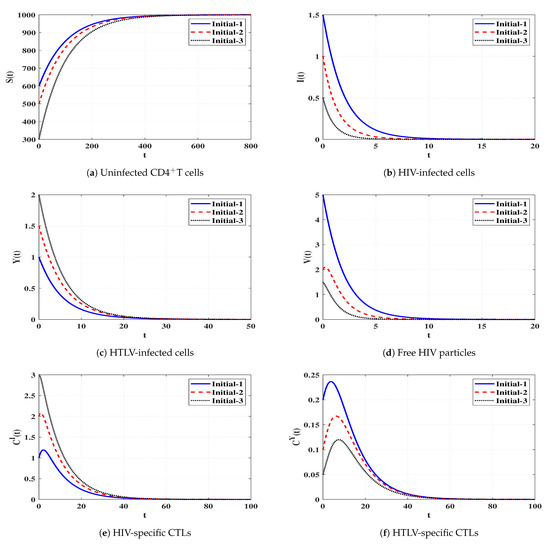
Figure 2. Solutions of system (4) when ℜ₁ ≤ 1 and ℜ₂ ≤ 1.

Set 2 (Stability of Đ${}_1$):${\eta }_1={\eta }_2=0.0005,$${\sigma }_1=0.003$ and ${\sigma }_2=0.2$. With such choice, we get ${\Re }_2=0.50<1<2.50={\Re }_1$, ${\Re }_3=0.48<1$ and hence ${\Re }_2/{\Re }_1=0.2<1$. The steady state Đ${}_1$ exists with Đ${}_1=(400,12,0,30,0,0)$, and the conditions given in Table 1 are verified. Figure 3 shows the stability of the system around Đ${}_1$ initiating from different states. Thus, the numerical simulations support the result obtained in Theorem 2. This leads to the situation of persistent HIV single infection but with an ineffective CTL immune response.

Figure 3. Solutions of system (4) when ℜ₁ > 1, ℜ₂/ℜ₁ ≤ 1 and ℜ₃ ≤ 1.

Set 3 (Stability of Đ${}_2$):${\eta }_1=0.0001,$${\eta }_2=0.002$, ${\sigma }_1=0.001$ and ${\sigma }_2=0.01$. Then, we calculate ${\Re }_1=0.50<1<2={\Re }_2$, ${\Re }_4=0.67<1$ and then ${\Re }_1/{\Re }_2=0.25<1$. It is obvious that the conditions mentioned in Table 1 are satisfied and Đ${}_2=(500,0,5,0,0,0)$. Figure 4 declares that the solutions of the system starting from different states tend to the steady state Đ${}_2$. This shows the consistency between the numerical results and theoretical result of Theorem 3. Thus, a persistent HTLV single infection with an ineffective CTL immune response will be reached.

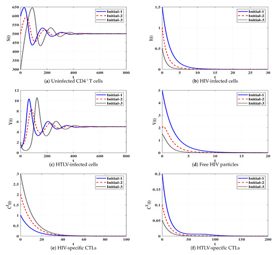
Figure 4. Solutions of system (4) when ℜ₂ > 1, ℜ₁/ℜ₂ ≤ 1 and ℜ₄ ≤ 1.

Set 4 (Stability of Đ${}_3$):${\eta }_1=0.001,$${\eta }_2=0.003$ and ${\sigma }_1={\sigma }_2=0.01$. Then, we calculate ${\Re }_3=1.43>1$ and ${\Re }_5=0.86<1$. From Table 1 and Figure 5, we conclude that the trajectories starting with different states tend to Đ${}_3=(285.83,10,0,24.97,1.07,0)$. Therefore, Đ${}_3$ is G.A.S, and this is compatible with Theorem 4. This leads to the case of persistent HIV single infection with an effective HIV-specific CTL immune response.

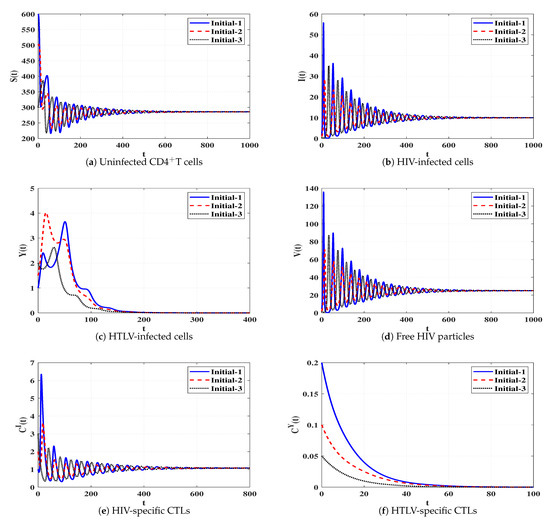
Figure 5. Solutions of system (4) when ℜ₃ > 1 and ℜ₅ ≤ 1.

Set 5 (Stability of Đ${}_4$):${\eta }_1=0.00025,$${\eta }_2=0.005$, ${\sigma }_1=0.05$ and ${\sigma }_2=0.02$. Then, we calculate ${\Re }_4=1.43>1$ and ${\Re }_6=0.36<1$. According to Table 1, Đ${}_4$ exists with Đ${}_4=(285.70,0,5,0,0,0.43)$. In Figure 6, we draw the solutions of the system with three different initial states. It is clear that Đ${}_4$ is G.A.S, which supports Theorem 5. In this case, a persistent HTLV single infection with effective HTLV-specific CTL is reached.

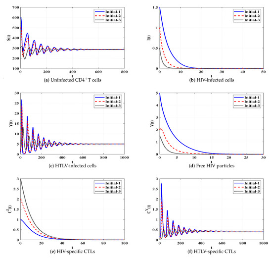
Figure 6. Solutions of system (4) when ℜ₄ > 1 and ℜ₆ ≤ 1.

Set 6 (Stability of Đ${}_5$):${\eta }_1=0.001,$${\eta }_2=0.0015$, ${\sigma }_1=0.15$ and ${\sigma }_2=0.033$. Then, we calculate ${\Re }_5=1.29>1$, ${\Re }_8=0.93<1$ and ${\Re }_1/{\Re }_2=3.33>1$. The numerical results demonstrated in Table 1 and Figure 7 show that Đ${}_5=(667.12,0.67,2.22,1.67,5.84,0)$ exists and based on Theorem 6, Đ${}_5$ is G.A.S. This case leads to a persistent dual infection with HTLV and HIV where the HIV-specific CTL is effective while the HTLV-specific CTL is ineffective.

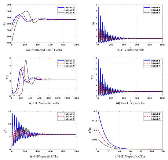
Figure 7. Solutions of system (4) when ℜ₅ > 1, ℜ₈ ≤ 1, and ℜ₁/ℜ₂ > 1.

Set 7 (Stability of Đ${}_6$):${\eta }_1=0.0007,$${\eta }_2=0.005$, ${\sigma }_1=0.005$ and ${\sigma }_2=0.1$. We compute ${\Re }_6=2.33>1$, ${\Re }_7=0.70<1$ and ${\Re }_2/{\Re }_1=1.43>1$. Based on the conditions in Table 1, the steady state Đ${}_6=(285.72,11.43,1,28.58,0,0.43)$ exists. In Figure 8, we plot the numerical solutions of the system and show that Đ${}_6$ is G.A.S (Theorem 7). This situation leads to a persistent dual infection with HTLV and HIV where the HTLV-specific CTL is effective and the HIV-specific CTL does not work.

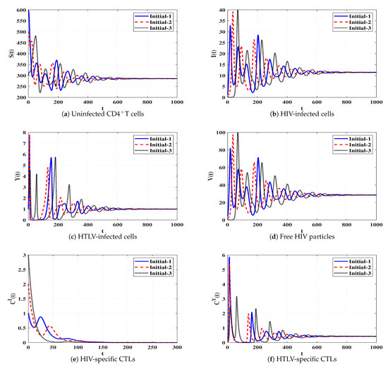
Figure 8. Solutions of system (4) when ℜ₆ > 1, ℜ₇ ≤ 1, and ℜ₂/ℜ₁ > 1.

Set 8 (Stability of Đ${}_7$):${\eta }_1=0.002,$${\eta }_2=0.0026$, ${\sigma }_1=0.04$ and ${\sigma }_2=0.1$. These data give ${\Re }_7=3.98>1$ and ${\Re }_8=1.04>1$. Based on the data mentioned in Table 1, the steady state Đ${}_7=(398.48,2.50,1,6.25,7.46,0.04)$ exists. Figure 9 illustrates that the solutions of the system initiating with three different states tend to Đ${}_7$. In this case, a persistent dual infection with HTLV and HIV is reached where both immune responses are well working.

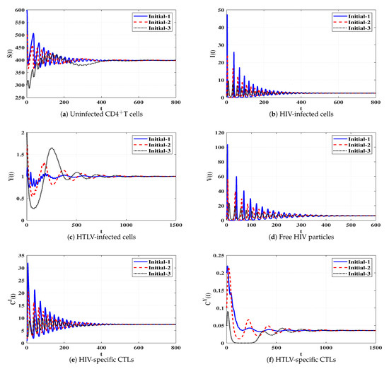
Figure 9. Solutions of system (4) when ℜ₇ > 1 and ℜ₈ > 1.

For further confirmation, we study the local stability of the system’s steady states. We first calculate the Jacobian matrix $J=J(S,I,Y,V,C^I,C^Y)$ of system (4) as:

$$J=\left(\begin{array}{cccccc}-\left(\alpha +{\eta }_{1}V+{\eta }_{2}Y\right)& 0& -{\eta }_{2}S& -{\eta }_{1}S& 0& 0\\ {\eta }_{1}V& -\left(a+{\mu }_1{C}^I\right)& 0& {\eta }_{1}S& -{\mu }_{1}I& 0\\ \phi {\eta }_{2}Y& 0& \phi {\eta }_{2}S-\left(\delta +{\mu }_2{C}^Y\right)& 0& 0& -{\mu }_{2}Y\\ 0& b& 0& -\epsilon & 0& 0\\ 0& {\sigma }_1{C}^I& 0& 0& {\sigma }_{1}I-{\pi }_1& 0\\ 0& 0& {\sigma }_2{C}^Y& 0& 0& {\sigma }_{2}Y-{\pi }_2\end{array}\right).$$

Then, we compute the eigenvalues ${\lambda }_i,$ $i=1,2,\dots ,6$ of J at each steady state. The steady state is locally stable if the eigenvalues satisfy $Re\left({\lambda }_i\right)<0,$ for all $i=1,2,\dots ,6$. We use the values of the parameters ${\eta }_1$, ${\eta }_2$, ${\sigma }_1$, and ${\sigma }_2$ given in Sets 1–8 and compute all non-negative steady states and the corresponding real parts of the eigenvalues (see Table 4). The local stability results agree with the global stability results given in Theorems 1–8.

Table 4. Local stability of positive steady state Đ${}_i$, $i=0,1,...,7$.

Set	$\begin{array}{c}\mathbf{Steady}\mathbf{States}\end{array}$	$\begin{array}{c}(Re\left({\mathit{\lambda }}_{\mathit{i}}\right),\mathit{i}=1,2,...,6)\end{array}$	$\begin{array}{c}\mathbf{Stability}\end{array}$
1	$\begin{array}{c}{Đ}_0=(1000,0,0,0,0,0)\end{array}$	$\begin{array}{c}\left(-2.28,-0.22,-0.1,-0.1,-0.1,-0.01\right)\end{array}$	$\begin{array}{c}\mathrm{stable}\hfill \end{array}$
2	$\begin{array}{c}{Đ}_0=(1000,0,0,0,0,0)\hfill \\ {Đ}_1=(400,12,0,30,0,0)\hfill \end{array}$	$\begin{array}{c}\left(-3,0.5,-0.1,-0.1,-0.1,-0.01\right)\hfill \\ \left(-2.5,-0.16,-0.1,-0.01,-0.01,-0.06\right)\hfill \end{array}$	$\begin{array}{c}\mathrm{unstable}\hfill \\ \mathrm{stable}\hfill \end{array}$
3	$\begin{array}{c}{Đ}_0=(1000,0,0,0,0,0)\hfill \\ {Đ}_2=(500,0,5,0,0,0)\hfill \end{array}$	$\begin{array}{c}\left(-2.28,-0.22,0.2,-0.1,-0.1,-0.01\right)\hfill \\ \left(-2.15,-0.35,-0.1,-0.05,-0.01,-0.01\right)\hfill \end{array}$	$\begin{array}{c}\mathrm{unstable}\hfill \\ \mathrm{stable}\hfill \end{array}$
4	$\begin{array}{c}{Đ}_0=(1000,0,0,0,0,0)\hfill \\ {Đ}_1=\left(200,16,0,40,0,0\right)\hfill \\ {Đ}_2=\left(333.33,0,6.67,0,0,0\right)\hfill \\ {Đ}_3=(285.83,10,0,24.97,1.07,0)\hfill \end{array}$	$\begin{array}{c}\left(-3.61,1.11,0.4,-0.1,-0.1,-0.01\right)\hfill \\ \left(-2.51,-0.02,-0.02,-0.1,-0.08,0.06\right)\hfill \\ \left(-2.74,0.24,-0.1,-0.02,-0.02,-0.03\right)\hfill \\ \left(-2.72,-0.01,-0.01,-0.1,-0.03,-0.02\right)\hfill \end{array}$	$\begin{array}{c}\mathrm{unstable}\hfill \\ \mathrm{unstable}\hfill \\ \mathrm{unstable}\hfill \\ \mathrm{stable}\hfill \end{array}$
5	$\begin{array}{c}{Đ}_0=(1000,0,0,0,0,0)\hfill \\ {Đ}_1=\left(800,4,0,10,0,0\right)\hfill \\ {Đ}_2=\left(200,0,8,0,0,0\right)\hfill \\ {Đ}_3=\left(888.89,2,0,5,0.28,0\right)\hfill \\ {Đ}_4=(285.70,0,5,0,0,0.43)\hfill \end{array}$	$\begin{array}{c}\left(-2.60,0.8,-0.1,-0.1,0.10,-0.01\right)\hfill \\ \left(-2.50,0.6,-0.1,0.1,-0.01,-0.01\right)\hfill \\ \left(-2.15,-0.35,-0.1,-0.03,-0.03,0.06\right)\hfill \\ \left(-2.56,0.69,-0.1,-0.001,-0.001,-0.01\right)\hfill \\ \left(-2.21,-0.29,-0.01,-0.01,-0.1,-0.02\right)\hfill \end{array}$	$\begin{array}{c}\mathrm{unstable}\hfill \\ \mathrm{unstable}\hfill \\ \mathrm{unstable}\hfill \\ \mathrm{unstable}\hfill \\ \mathrm{stable}\hfill \end{array}$
6	$\begin{array}{c}{Đ}_0=(1000,0,0,0,0,0)\hfill \\ {Đ}_1=\left(200,16,0,40,0,0\right)\hfill \\ {Đ}_2=\left(666.67,0,3.33,0,0,0\right)\hfill \\ {Đ}_3=\left(857.14,0.67,0,1.67,8.21,0\right)\hfill \\ {Đ}_4=\left(687.5,0,3.03,0,0,0.03\right)\hfill \\ {Đ}_5=(667.12,0.67,2.22,1.67,5.84,0)\hfill \end{array}$	$\begin{array}{c}\left(-3.61,1.11,0.1,-0.1,-0.1,-0.01\right)\hfill \\ \left(-2.51,2.3,-0.14,-0.02,-0.02,-0.1\right)\hfill \\ \left(-3.22,0.72,-0.1,-0.01,-0.01,0.01\right)\hfill \\ \left(-4.12,-0.01,-0.01,-0.1,0.06,-0.01\right)\hfill \\ \left(-3.25,0.75,-0.1,-0.004,-0.004,-0.01\right)\hfill \\ \left(-3.65,-0.01,-0.01,-0.03,-0.01,-0.01\right)\hfill \end{array}$	$\begin{array}{c}\mathrm{unstable}\hfill \\ \mathrm{unstable}\hfill \\ \mathrm{unstable}\hfill \\ \mathrm{unstable}\hfill \\ \mathrm{unstable}\hfill \\ \mathrm{stable}\hfill \end{array}$
7	$\begin{array}{c}{Đ}_0=(1000,0,0,0,0,0)\hfill \\ {Đ}_1=\left(285.71,14.29,0,35.71,0,0\right)\hfill \\ {Đ}_2=\left(200,0,8,0,0,0\right)\hfill \\ {Đ}_4=\left(666.67,0,1,0,0,2.33\right)\hfill \\ {Đ}_6=(285.72,11.43,1,28.58,0,0.43)\hfill \end{array}$	$\begin{array}{c}\left(-3.27,0.8,0.77,-0.1,-0.1,-0.01\right)\hfill \\ \left(-2.50,-0.1,-0.02,-0.01,0.09,-0.03\right)\hfill \\ \left(-2.37,0.7,-0.13,-0.1,-0.025,-0.025\right)\hfill \\ \left(-2.95,0.45,-0.0004,-0.0004,-0.1,-0.01\right)\hfill \\ \left(-2.50,-0.01,-0.01,-0.01,-0.01,-0.04\right)\hfill \end{array}$	$\begin{array}{c}\mathrm{unstable}\hfill \\ \mathrm{unstable}\hfill \\ \mathrm{unstable}\hfill \\ \mathrm{unstable}\hfill \\ \mathrm{stable}\hfill \end{array}$
8	$\begin{array}{c}{Đ}_0=(1000,0,0,0,0,0)\hfill \\ {Đ}_1=\left(100,18,0,45,0,0\right)\hfill \\ {Đ}_2=\left(384.62,0,6.15,0,0,0\right)\hfill \\ {Đ}_3=\left(444.44,2.5,0,6.25,8.61,0\right)\hfill \\ {Đ}_4=\left(793.65,0,1,0,0,1.06\right)\hfill \\ {Đ}_5=\left(384.62,2.5,1.35,6.25,7.12,0\right)\hfill \\ {Đ}_7=(398.48,2.50,1,6.25,7.46,0.04)\hfill \end{array}$	$\begin{array}{c}\left(-4.5,2,0.32,-0.1,-0.1,-0.01\right)\hfill \\ \left(-2.51,0.62,-0.04,-0.04,-0.15,-0.1\right)\hfill \\ \left(-3.35,0.85,0.52,-0.1,-0.01,-0.01\right)\hfill \\ \left(-4.20,-0.01,-0.01,-0.1,0.03,-0.02\right)\hfill \\ \left(-4.17,1.67,-0.0003,-0.0003,-0.1,-0.01\right)\hfill \\ \left(-3.91,-0.01,-0.01,0.03,-0.01,-0.01\right)\hfill \\ \left(-3.98,-0.01,-0.01,-0.004,-0.004,-0.01\right)\hfill \end{array}$	$\begin{array}{c}\mathrm{unstable}\hfill \\ \mathrm{unstable}\hfill \\ \mathrm{unstable}\hfill \\ \mathrm{unstable}\hfill \\ \mathrm{unstable}\hfill \\ \mathrm{unstable}\hfill \\ \mathrm{stable}\hfill \end{array}$

6.2. Comparison Study

In this part, we make a comparison between single and dual infection dynamics.

Influence of HTLV infection on the dynamics of HIV single infection

To study the effect of HTLV infection on the dynamics of HIV single infection, we make a comparison between model (2) and (4). We select ${\eta }_1=0.002$, ${\eta }_2=0.005,$ ${\sigma }_1=0.02$, and ${\sigma }_2=0.04$ and take the following initial condition:

Initial-4:$(300,4,1.5,10,3,0.05)$.

Figure 10 shows that, if an individual who only has HIV infection is dually infected with HTLV, then the concentrations of uninfected CD$4^{+}$T cells and HIV-specific CTLs are decayed, while the concentration of free HIV particles reaches the same value in both HIV single infection and HTLV/HIV dual infection. In fact, this observation is consistent with the recent study [50], where it has been found that there are no noteworthy differences in the concentration of HIV particles in comparisons between HIV single infected and HTLV/HIV dual infected patients.

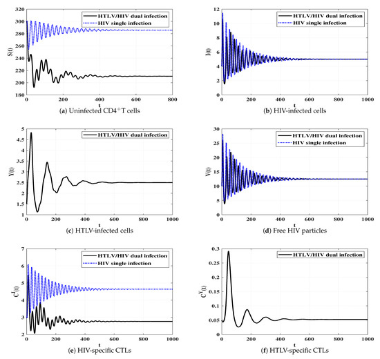
Figure 10. Comparison between the dynamics of HIV single infection and HTLV/HIV dual infection.

Influence of HIV infection on the dynamics of HTLV single infection

To see the effect of HIV infection on the dynamics of HTLV single infection, we perform a comparison between models (3) and (4).

We select the values ${\eta }_1=$ $0.001,$ ${\eta }_2=0.006$, ${\sigma }_1=0.027$, and ${\sigma }_2=0.02$ and take the following initial state:

Initial-5:$=(220,3.5,5,9,0.03,0.35)$.

Figure 11 displays the solutions of two systems (3) and (4). We observe that the concentrations of uninfected CD$4^{+}$T cells and HTLV-specific CTLs are smaller in the case of dual infection than that of HTLV single infection. In contrast, the concentration of HTLV-infected cells reaches the same value in both HTLV single and HTLV/HIV dual infections.

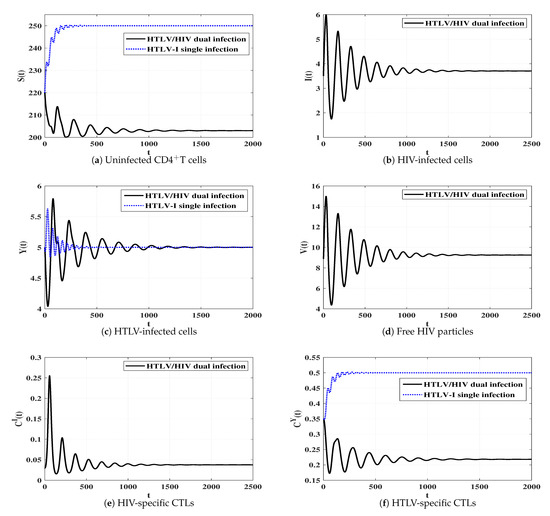
Figure 11. Comparison between the dynamics of HTLV-I single infection and HTLV/HIV dual infection.

7. Conclusions and Discussions

This work proposes and investigates a within host HTLV/HIV dual infection model. The model contains six compartments, uninfected CD$4^{+}$T cells, HIV-infected cells, free HIV particles, HIV-specific CTLs, HTLV-infected cells, and HTLV-specific CTLs. HIV was assumed to be transmitted through free-to-cell touch, while the HTLV was transmitted via direct infected-to-cell touch. We first showed that the model is biologically acceptable by proving that the solutions are non-negative and bounded. We calculated eight steady states in which their existence and stability are determined by eight threshold parameters. We constructed suitable Lyapunov functions and applied the Lyapunov–LaSalle asymptotic stability theorem to prove the global asymptotic stability of all steady states. We solved the system numerically and concluded that both theoretical and numerical results are matched. We compared between the dynamical behavior of single HTLV (or HIV) infection and dual HTLV/HIV infection. The model analysis suggested that dual infected individuals with both viruses will have a smaller number of uninfected CD$4^{+}$T cells in comparison with HIV or HTLV single infected individuals.

Our model can be extended in many directions:

• In model (4), we supposed that uninfected CD$4^{+}$T cells are created at a constant rate $\rho$ and die at linear rate $\alpha S$. In fact, it would be more acceptable to examine the density dependent creation rate. One possibility is to consider a logistic growth for the uninfected CD$4^{+}$T cells. Moreover, the model assumed bilinear incidence rate of infection. However, such bilinear form may not describe the virus dynamics during the full course of infection. Therefore, it is reasonable to consider other forms of the incidence rate such as: saturated incidence, Beddington–DeAngelis incidence and general incidence [51].
• Model (4) assumed that once uninfected CD$4^{+}$T cells are contacted by HIV particles or HTLV-infected cells, they become infected instantaneously. However, such a process needs time. The effect of intracellular time delay on the dynamics of dual infection has a significant importance. Delayed single virus infection models have been formulated and analyzed in many articles (see, e.g., [52,53,54,55,56]). Another way to include such delay period is to consider two types of infected cells: latent and active [45].
• Model (4) supposes that the viruses and cells are equally distributed in the domain with no spatial variations. Taking into account spatial variations in the case of HTLV/HIV dual infection will be significant [16,57].
  We mention that these extensions may increase the numbers of parameters, and this requires a large number of measurements (blood samples) for estimation of the parameters.

We leave these extensions as future work.

It is well known that CTLs play a significant role in controlling HTLV and HIV single infections by killing infected cells. When the CTL immunity is not considered, model (4) leads to a model with competition between HTLV and HIV on CD$4^{+}$T cells:

$$\left\{\begin{array}{c}\frac{dS}{dt}=\rho -\alpha S-{\eta }_{1}SV-{\eta }_{2}SY,\hfill \\ \frac{dI}{dt}={\eta }_{1}SV-aI,\hfill \\ \frac{dY}{dt}=\phi {\eta }_{2}SY-\delta Y,\hfill \\ \frac{dV}{dt}=bI-\epsilon V.\hfill \end{array}\right.$$

(22)

This system has only three steady states: infection-free steady state, ${\overline{Đ}}_0=(S_0,0,0,0)$, persistent HIV single infection steady state, ${\overline{Đ}}_1=(S_1,I_1,0,V_1)$, and persistent HTLV single infection steady state, ${\overline{Đ}}_2=(S_2,0,Y_2,0)$, where $S_0$, $S_1$, $I_1$, $V_1$, $S_2$ and $Y_2$ are given in Section 4. The existence of these three steady states is determined by two threshold parameters ${\Re }_1$ and ${\Re }_2$, which are also defined in Section 4.

Corollary 1.

For system (22), the following statements hold true.

(i) 

If ${\Re }_1\le 1$ and ${\Re }_2\le 1$, then ${\overline{Đ}}_0$ is G.A.S.

(ii) 

If ${\Re }_1>1$ and ${\Re }_2/{\Re }_1\le 1$, then ${\overline{Đ}}_1$ is G.A.S.

(iii) 

If ${\Re }_2>1$ and ${\Re }_1/{\Re }_2\le 1$, then ${\overline{Đ}}_2$ is G.A.S.

Therefore, the system will tend to one of the three steady states ${\overline{Đ}}_0$, ${\overline{Đ}}_1$ and ${\overline{Đ}}_2$. The above result says that, in the absence of CTL immunity, in the competition between HTLV and HIV consuming common resources, only one type of viruses with maximum basic reproduction number can survive. However, in our proposed model (4) involving HIV- and HTLV-specific CTLs, HTLV and HIV coexist in a steady state. We can consider this situation as follows. Since CTL immune responses suppress viral progression, the competition between HTLV and HIV is also suppressed, and the coexistence of HTLV and HIV occurs [58].

It has been reported in [4] that HIV has two classes of target cells, CD$4^{+}$T cells and macrophages. In this case, HIV has two resources and then the coexistence of HTLV and HIV can occur even when the immune system is workless. HIV single infection models with two classes of target cells have been studied in several works (see, e.g., [6,10]) Therefore, our model can be extended to take into account the second class of target cells for HIV, macrophages. We leave this extension for future works.

References

- Burger, H.; Belman, A.L.; Grimson, R.; Kaell, A.; Flaherty, K.; Gulla, J.; Gibbs, R.A.; Nguyun, P.N.; Weiser, B. Long HIV-1 incubation periods and dynamics of transmission within a family. Lancet 1990, 336, 134–136. [Google Scholar] [CrossRef]
- Nowak, M.A.; May, R.M. Virus Dynamics: Mathematical Principles of Immunology and Virology; Oxford University Press: Oxford, UK, 2000. [Google Scholar]
- Nowak, M.A.; Bangham, C.R.M. Population dynamics of immune responses to persistent viruses. Science 1996, 272, 74–79. [Google Scholar] [CrossRef] [PubMed]
- Perelson, A.S.; Essunger, P.; Cao, Y.; Vesanen, M.; Hurley, A.; Saksela, K.; Markowitz, M.; Ho, D.D. Decay characteristics of HIV-1-infected compartments during combination therapy. Nature 1997, 387, 188–191. [Google Scholar] [CrossRef] [PubMed]
- Perelson, A.S.; Nelson, P.W. Mathematical analysis of HIV-1 dynamics in vivo. SIAM Rev. 1999, 41, 3–44. [Google Scholar] [CrossRef]
- Callaway, D.S.; Perelson, A.S. HIV-1 infection and low steady state viral loads. Bull. Math. Biol. 2002, 64, 29–64. [Google Scholar] [CrossRef]
- Rong, L.; Perelson, A.S. Modeling HIV persistence, the latent reservoir, and viral blips. J. Theor. 2009, 260, 308–331. [Google Scholar] [CrossRef]
- Wang, L.; Li, M.Y. Mathematical analysis of the global dynamics of a model for HIV infection of CD4+ T cells. Math. Biosci. 2006, 200, 44–57. [Google Scholar] [CrossRef]
- Li, D.; Ma, W. Asymptotic properties of a HIV-1 infection model with time delay. J. Math. Anal. Appl. 2007, 335, 683–691. [Google Scholar] [CrossRef]
- Elaiw, A.M. Global properties of a class of HIV models. Nonlinear Anal. Real World Appl. 2010, 11, 2253–2263. [Google Scholar] [CrossRef]
- Huang, G.; Liu, X.; Takeuchi, Y. Lyapunov functions and global stability for age-structured HIV infection model. SIAM J. Appl. Math. 2012, 72, 25–38. [Google Scholar] [CrossRef]
- Elaiw, A.M.; Alshaikh, M.A. Stability of discrete-time HIV dynamics models with three categories of infected CD4+ T-cells. Adv. Differ. Equ. 2019, 2019, 407. [Google Scholar] [CrossRef]
- Elaiw, A.M.; AlShamrani, N.H. Stability of a general CTL-mediated immunity HIV infection model with silent infected cell-to-cell spread. Adv. Differ. Equ. 2020, 2020, 355. [Google Scholar] [CrossRef]
- Elaiw, A.M.; Almuallem, N.A. Global dynamics of delay-distributed HIV infection models with differential drug efficacy in cocirculating target cells. Math. Methods Appl. Sci. 2016, 39, 4–31. [Google Scholar] [CrossRef]
- Liu, H.; Zhang, J.-F. Dynamics of two time delays differential equation model to HIV latent infection. Physica A 2019, 514, 384–395. [Google Scholar] [CrossRef]
- Bellomo, N.; Painter, K.J.; Tao, Y.; Winkler, M. Occurrence vs. Absence of taxis-driven instabilities in a May-Nowak model for virus infection. SIAM J. Appl. Math. 2019, 79, 1990–2010. [Google Scholar] [CrossRef]
- Chen, W.; Tuerxun, N.; Teng, Z. The global dynamics in a wild-type and drug-resistant HIV infection model with saturated incidence. Adv. Differ. Equ. 2020, 2020, 25. [Google Scholar] [CrossRef]
- Norrgren, H.R.; Bamba, S.; Larsen, O.; Da Silva, Z.; Aaby, P.; Koivula, T.; Andersson, S. Increased prevalence of HTLV-1 in patients with pulmonary tuberculosis coinfected with HIV, but not in HIV-negative patients with tuberculosis. J. Acquir. Immune Defic. Syndr. 2008, 48, 607–610. [Google Scholar] [CrossRef]
- Pan, X.; Chen, Y.; Shu, H. Rich dynamics in a delayed HTLV-I infection model: Stability switch, multiple stable cycles, and torus. J. Math. Anal. Appl. 2019, 479, 2214–2235. [Google Scholar] [CrossRef]
- Yamamoto, N.; Okada, M.; Koyanagi, Y.; Kannagi, M.; Hinuma, Y. Transformation of human leukocytes by cocultivation with an adult T cell leukemia virus producer cell line. Science 1982, 217, 737–739. [Google Scholar] [CrossRef]
- Asquith, B.; Bangham, C.R.M. The dynamics of T-cell fratricide: Application of a robust approach to mathematical modeling in immunology. J. Theor. Biol. 2003, 222, 53–69. [Google Scholar] [CrossRef]
- Tokudome, S.; Tokunaga, O.; Shimamoto, Y.; Miyamoto, Y.; Sumida, I.; Kikuchi, M.; Takeshita, M.; Ikeda, T.; Fujiwara, K.; Yoshihara, M.; et al. Incidence of adult T cell leukemia/lymphoma among human T lymphotropic virus type 1 carriers in Saga, Japan. Cancer Res. 1989, 49, 226–228. [Google Scholar] [PubMed]
- Stilianakis, N.I.; Seydel, J. Modeling the T-cell dynamics and pathogenesis of HTLV-I infection. Bull. Math. Biol. 1999, 61, 935–947. [Google Scholar] [CrossRef] [PubMed]
- Gomez-Acevedo, H.; Li, M.Y. Backward bifurcation in a model for HTLV-I infection of CD4+ T cells. Bull. Math. Biol. 2005, 67, 101–114. [Google Scholar] [CrossRef] [PubMed]
- Vargas-De-Leon, C. The complete classification for global dynamics of amodel for the persistence of HTLV-1 infection. Appl. Math. Comput. 2014, 237, 489–493. [Google Scholar]
- Li, M.Y.; Lim, A.G. Modelling the role of Tax expression in HTLV-1 persisence in vivo. Bull. Math. Biol. 2011, 73, 3008–3029. [Google Scholar] [CrossRef] [PubMed]
- Song, X.; Li, Y. Global stability and periodic solution of a model for HTLV-1 infection and ATL progression. Appl. Math. Comput. 2006, 180, 401–410. [Google Scholar] [CrossRef]
- Wang, L.; Li, M.Y.; Kirschner, D. Mathematical analysis of the global dynamics of a model for HTLV-I infection and ATL progression. Math. Biosci. 2002, 179, 207–217. [Google Scholar] [CrossRef]
- Asquith, B.; Bangham, C.R.M. Quantifying HTLV-I dynamics. Immunol. Cell Biol. 2007, 85, 280–286. [Google Scholar] [CrossRef]
- Bartholdy, C.; Christensen, J.P.; Wodarz, D.; Thomsen, A.R. Persistent virus infection despite chronic cytotoxic T-lymphocyte activation in gamma interferon-deficient mice infected with lymphocytic choriomeningitis virus. J. Virol. 2000, 74, 10304–10311. [Google Scholar] [CrossRef]
- Wodarz, D.; Bangham, C.R.M. Evolutionary dynamics of HTLV-I. J. Mol. Evol. 2000, 50, 448–455. [Google Scholar] [CrossRef]
- Gomez-Acevedo, H.; Li, M.Y.; Jacobson, S. Multi-stability in a model for CTL response to HTLV-I infection and its consequences in HAM/TSP development, and prevention. Bull. Math. 2010, 72, 681–696. [Google Scholar] [CrossRef] [PubMed]
- Lang, J.; Li, M.Y. Stable and transient periodic oscillations in a mathematical model for CTL response to HTLV-I infection. J. Math. Biol. 2012, 65, 181–199. [Google Scholar] [CrossRef] [PubMed]
- Li, M.Y.; Shu, H. Global dynamics of a mathematical model for HTLV-I infection of CD4+ T cells with delayed CTL response. Nonlinear Anal. Real World Appl. 2012, 13, 1080–1092. [Google Scholar] [CrossRef]
- Wang, L.; Liu, Z.; Li, Y.; Xu, D. Complete dynamical analysis for a nonlinear HTLV-I infection model with distributed delay, CTL response and immune impairment. Discret. Contin. Dyn. 2020, 25, 917–933. [Google Scholar] [CrossRef]
- Muroya, Y.; Enatsu, Y.; Li, H. Global stability of a delayed HTLV-I infection model with a class of nonlinear incidence rates and CTLs immune response. Appl. Math. Comput. 2013, 219, 10559–10573. [Google Scholar] [CrossRef]
- Wang, Y.; Liu, J.; Heffernan, J.M. Viral dynamics of an HTLV-I infection model with intracellular delay and CTL immune response delay. J. Math. Anal. Appl. 2018, 459, 506–527. [Google Scholar] [CrossRef]
- Li, F.; Ma, W. Dynamics analysis of an HTLV-1 infection model with mitotic division of actively infected cells and delayed CTL immune response. Math. Methods Appl. Sci. 2018, 41, 3000–3017. [Google Scholar] [CrossRef]
- Casoli, C.; Pilotti, E.; Bertazzoni, U. Molecular and cellular interactions of HIV-1/HTLV coinfection and impact on AIDS progression. AIDS Rev. 2007, 9, 140–149. [Google Scholar]
- Silva, M.T.; Espíndola, O.D.; Leite, A.C.; Araújo, A. Neurological aspects of HIV/human T lymphotropic virus coinfection. AIDS Rev. 2009, 11, 71–78. [Google Scholar]
- Brites, C.; Sampalo, J.; Oliveira, A. HIV/human T-cell lymphotropic virus coinfection revisited: Impact on AIDS progression. AIDS Rev. 2009, 11, 8–16. [Google Scholar]
- Isache, C.; Sands, M.; Guzman, N.; Figueroa, D. HTLV-1 and HIV-1 co-infection: A case report and review of the literature. IDCases 2016, 4, 53–55. [Google Scholar] [CrossRef] [PubMed]
- Beilke, M.A.; Theall, K.P.; O’Brien, M.; Clayton, J.L.; Benjamin, S.M.; Winsor, E.L.; Kissinger, P.J. Clinical outcomes and disease progression among patients coinfected with HIV and human T lymphotropic virus types 1 and 2. Clin. Infect. Dis. 2004, 39, 256–263. [Google Scholar] [CrossRef] [PubMed]
- Elaiw, A.M.; AlShamrani, N.H. Analysis of a within-host HIV/HTLV-I co-infection model with immunity. Virus Res. 2020, 198204. [Google Scholar] [CrossRef] [PubMed]
- Korobeinikov, A. Global properties of basic virus dynamics models. Bull. Math. Biol. 2004, 66, 879–883. [Google Scholar] [CrossRef]
- Hale, J.K.; Lunel, S.V. Introduction to Functional Differential Equations; Springer: New York, NY, USA, 1993. [Google Scholar]
- Barbashin, E.A. Introduction to the Theory of Stability; Wolters-Noordhoff: Groningen, The Netherlands, 1970. [Google Scholar]
- LaSalle, J.P. The Stability of Dynamical Systems; SIAM: Philadelphia, PA, USA, 1976. [Google Scholar]
- Lyapunov, A.M. The General Problem of the Stability of Motion; Taylor & Francis, Ltd.: London, UK, 1992. [Google Scholar]
- Vandormael, A.; Rego, F.; Danaviah, S.; Alcantara, L.C.; Boulware, D.R.; de Oliveira, T. CD4+ T-cell count may not be a useful strategy to monitor antiretroviral therapy response in HTLV-1/HIV co-infected patients. Curr. HIV Res. 2017, 15, 225–231. [Google Scholar] [CrossRef]
- Huang, G.; Takeuchi, Y.; Ma, W. Lyapunov functionals for delay differential equations model of viral infections. SIAM J. Appl. Math. 2010, 70, 2693–2708. [Google Scholar] [CrossRef]
- Nelson, P.W.; Murray, J.D.; Perelson, A.S. A model of HIV-1 pathogenesis that includes an intracellular delay. Math. Biosci. 2000, 163, 201–215. [Google Scholar] [CrossRef]
- Elaiw, A.M.; AlShamrani, N.H. Global stability of a delayed adaptive immunity viral infection with two routes of infection and multi-stages of infected cells. Commun. Nonlinear Sci. Numer. Simul. 2020, 86, 105259. [Google Scholar] [CrossRef]
- Elaiw, A.M.; Alshehaiween, S.F.; Hobiny, A.D. Global properties of a delay-distributed HIV dynamics model including impairment of B-cell functions. Mathematics 2019, 7, 837. [Google Scholar] [CrossRef]
- Elaiw, A.M.; Elnahary, E.K. Analysis of general humoral immunity HIV dynamics model with HAART and distributed delays. Mathematics 2019, 7, 157. [Google Scholar] [CrossRef]
- Culshaw, R.V.; Ruan, S.; Webb, G. A mathematical model of cell-to-cell spread of HIV-1 that includes a time delay. J. Math. Biol. 2003, 46, 425–444. [Google Scholar] [CrossRef] [PubMed]
- Elaiw, A.M.; AlAgha, A.D. Global analysis of a reaction-diffusion within-host malaria infection model with adaptive immune response. Mathematics 2020, 8, 563. [Google Scholar] [CrossRef]
- Inoue, T.; Kajiwara, T.; Saski, T. Global stability of models of humoral immunity against multiple viral strains. J. Biol. Dyn. 2010, 4, 282–295. [Google Scholar] [CrossRef] [PubMed]
Publisher’s Note: MDPI stays neutral with regard to jurisdictional claims in published maps and institutional affiliations. |
© 2020 by the authors. Licensee MDPI, Basel, Switzerland. This article is an open access article distributed under the terms and conditions of the Creative Commons Attribution (CC BY) license (http://creativecommons.org/licenses/by/4.0/).