Article

Classifying a Lending Portfolio of Loans with Dynamic Updates via a Machine Learning Technique

by
Fazlollah Soleymani
1,
Houman Masnavi
2 and
Stanford Shateyi
3,*
1
Department of Mathematics, Institute for Advanced Studies in Basic Sciences (IASBS), Zanjan 45137-66731, Iran
2
Intelligent Materials and Systems Lab, University of Tartu, 50411 Tartu, Estonia
3
Department of Mathematics and Applied Mathematics, School of Mathematical and Natural Sciences, University of Venda, P. Bag X5050, Thohoyandou 0950, South Africa
*
Author to whom correspondence should be addressed.
Mathematics 2021, 9(1), 17; https://doi.org/10.3390/math9010017
Submission received: 16 November 2020 / Revised: 8 December 2020 / Accepted: 16 December 2020 / Published: 23 December 2020
(This article belongs to the Special Issue Financial Modeling)

Abstract

:
Bankruptcy prediction has been broadly investigated using financial ratios methodologies. One involved factor is the quality of the portfolio of loans which is given. Hence, having a model to classify/predict position of each loan candidate based on several features is important. In this work, an application of machine learning approach in mathematical finance and banking is discussed. It is shown how we can classify some lending portfolios of banks under several features such as rating categories and various maturities. Dynamic updates of the portfolio are also given along with the top probabilities showing how the financial data of this type can be classified. The discussions and results reveal that a good algorithm for doing such a classification on large economic data of such type is the k-nearest neighbors (KNN) with k = 1 along with parallelization even over the support vector machine, random forest, and artificial neural network techniques to save as much as possible on computational time.
MSC:
91G60; 91G99
JEL Classification:
C52; C82; H81

1. Introduction

Consider a financial institution which requires evaluating and assessing the quality and performance of a large portfolio giving loans to clients throughout a country. Since the lending portfolio provides a huge number of loans under different types of conditions to various clients and in some cases the number of loans might exceed millions, it would be time-consuming to apply traditional statistical approaches for evaluating the quality of such a portfolio [1]. On the other hand, there are cases at which all the features for distinguishing the banking data are not given, and this leads to relying on new approaches for classification and finding patterns in the economic and financial data. Classification is the process of putting items into predetermined sets. This process is also called as the pattern recognition [2].
As such, determining a mechanism for exploring and arranging the large data into groups of information is a significant and difficult task. In this circumstance, an application of artificial intelligence (AI) techniques comes into play because of its quick performance and sufficient accuracy under some conditions. To achieve this, several prominent machine-learning-based methods (e.g., refer to [3] and its references), viz., radial basis function regression (RBFR), multiple linear regression (MLR), support vector machine (SVM) [4], random forest (RF) [5,6], k-nearest neighbors (KNN), and random tree (RT) were used and applied in engineering problems [7,8,9]. The ML field has been developing at a rapid pace and the recent breakthroughs in data storage and calculating power have made it ubiquitous across a plethora of various applications, many of which are prevalent, see [10] and the references cited therein. The link between machine learning (ML) field and the computational mathematics has recently been discussed in detail in terms of mathematical background in [11].
Recently, the authors in [12] discussed the accuracy of two different ways, i.e., the traditional statistical techniques—such as logistic regression and discriminant analysis-and the ML techniques (artificial neural network (ANN), SVMs, and KNN) to predict banks’ failure. Actually, a set of 3000 US banks (1562 active banks and 1438 failures) was examined by these approaches, see [13] for more. For each bank, data were gathered on a five-year period. Then, thirty one financial ratios reported by the banks contained the five main aspects: profitability, liquidity, operations efficiency, capital quality, and loan quality. For the failed-bank assets, The cost per dollar is already high and can be increased [12,14]. As such, The more banks go bankrupt, The higher the cost of handling after-failure events. At the end of 2013, The corporation stated that approximately the whole cost to the deposit insurance funds for resolving these failed banks is more than 30 billion USD. Hence, detection of bank failure prior to it happening is necessary [15,16].
As another example, when a business applies for a loan, The lender should examine if it is able to return the loan interest and principal. Lenders often use leverage and profitability criteria to evaluate the credit risk, see, e.g., [17,18]. a lucrative firm is one with enough turnover to cover principal due and interest expense. To discuss further, given two loan requesters—one with high profitability and high leverage, and another one with low profitability and low leverage, we want to know which firm has lower credit risk? The challenges of responding to this query multiply when banks impose several other dimensions they consider during credit risk assessment. These extra dimensions normally consist of other financial information like liquidity ratio, or behavioral information like loan/trade credit payment behavior. Encompassing all of these various dimensions into a single core is intensive, but the ML methods help overcome this [19].
Single-label and multi-label classifiers are tested in [20], demonstrating that multi-label classifiers perform better. In addition, The ML methods furnish a better fit for the nonlinear relations between the default risk and explanatory variables [21]. See also [22] for further discussions.
This paper adds further discussions in the growing body of knowledge on using ML techniques for a financial problem by asking whether different values for the free integer parameter k in the nearest neighbors technique can be used to predict the behavior of lending portfolio of loans. Additionally, this work considers a broader range of scenarios in which a financial manager wishes to predict the behavior of the lending portfolio in contrast to [23]. Dynamic updates on the portfolio will also be furnished to show the applicability of the ML approach in classifying large banking data.
In this paper, we contribute by furnishing an ML-based model for a bank manager who wishes to classify all loan requesters as efficient as possible by considering three features, including loan’s maturity rate, The client’s credit spread, and remaining spread. We use ML because of the presence of a large amount of data as well. Different algorithms are used for classifying and putting loans into their respective risk categories, and the ones resulting in more pronounced outcomes are compared against each other. It is shown that KNN with appropriate k outperforms other algorithms for the application scenario presented in this paper. To discuss further, there are many efficient classifiers for financial engineering problems in literature, see e.g., [24]. However, The motivation of choosing KNN is that we employed several techniques, such as KNN, with six different k, RF, SVM, and ANN, To do this classification problem with three features and finally observed that KNN with k = 1 performs better than the others. Obviously for other financial engineering situations, other techniques such as extreme gradient boosting or extreme learning machine could be employed [25].
The organization of this article is given as follows. Some discussions about the definitions and required materials from ML as a subset of AI is furnished in Section 2. Then, a lending portfolio (of loans) is defined in Section 3 along with its features in this study. Here, we consider three important features which are linked to each other in the lending portfolio. Furthermore, we take into consideration that there are six ranking categories for the position of loans. In fact, our main aim is to manage the risk of a financial institution such as banks for loan candidates by putting them in appropriate groups based on their riskiness situation. In Section 4, we execute the KNN ML technique and compare computationally how and under what conditions the new obtained model assesses the quality of lending portfolios and improves the prediction of bank failure. The results obtained show that the KNN algorithm with k = 1 , in comparison to RF, SVM, and ANN algorithms, is an efficient tool for assessing the quality of lending portfolios under several features. Finally, The summary is furnished in Section 5.

2. Background on Machine Learning

2.1. ML

Classification is considered as one of the analytical tools to extract information from data [2]. in fact, classification is a data-mining technique which is quite useful for finding patterns in economic and financial data. ML is considered as portion of AI which interlinks and uses several ideas coming from statistics, numerical analysis, and algorithms to ‘learn’ from data [26]. However, this learning process is mainly based on two reasonings, called as induction and deduction. Induction is mostly applied for obtaining and constructing classification rules while deduction is dealt with reasoning using existing knowledge. It is necessary to recall here that deduction is mainly used for prediction while ML is based upon induction. This means that it can lead to two issues as follows:
  • This type of learning through induction needs a lot of instances to get good knowledge.
  • Since the process of learning is based upon the events that happened previously, there would not be a 100% guarantee to get a very accurate model for predicting in the future.
In this work, we rely on learning by supervision which means that there is a supervisor continually assessing the classifier’s performance. Hence, a training set must be defined to let the original data set to be trained on. a training data set is a data set of examples used for learning that is to fit the parameters of, for instance, a classifier. in other words, The set of samples for which the features and measurements are known is denoted as the set of training.
Pattern recognition methods are divided into two branches:
  • Nonparametric discriminants [27]. a method of this category is the ANN, which tries to divide the original data space into various regions. In the simple case of a binary classification technique, The space of data is put into two areas.
  • Similarity-based classifiers [10]. Since the financial data sets basically include more variables than samples, such techniques are more used in financial applications.
The KNN is a nonparametric method with similarity-based measures. Classification techniques can be efficiently applied and considered in the risk management and large data set processing, at which group information is of special interest for the trader/investigator. as an example, recently, Hlivka in the work [23] discussed how ML can be applied on a set of large economic data coming from banks in lending portfolios having two features.

2.2. KNN

The KNN classifier infers the class of a new instance via analyzing its nearest neighbors in the feature space and calculating the Euclidean distance to each of its neighbors, after which it utilizes a majority voting technique to classify the example. in its simplest form, it picks the commonest class amongst the KNN. for instance, for a given y to be queried, with a training set of T = { x j } j = 1 N , and classes label of c 1 , c 2 , c n , where N is the number of samples, x j is the training sample, and n is the number of classes available, The KNN algorithm first calculates the Euclidean distances between the searching point and the training samples as follows [28]:
E d ( y , x j ) = ( y x j ) * ( y x j ) ,
wherein E d ( y , x j ) is the Euclidean distance of y from x j . Then, The distances are sorted in an ascending order. At the end, The majority voting would be performed to determine the query point’s class as follows:
y = arg max ( x j N ) w c M ,
where the weight, w, can be specified as follows:
w = 1 , c M = x j N , 0 , otherwise ,
with c M as the class label determined by majority voting. The mathematical convergence of this algorithm in a probability space was discussed in [29].
There are several methods for performing nearest neighbor search, viz., k-d tree (shortened for k-dimensional tree), Octree, and Scan. k-d tree is a binary tree that all of its leaves have k-dimensional points, and it can be implemented on data of various dimensions [30].
Performing a KNN search on k-d tree would be achieved as follows (in [31] Appendix B): 1. Starting from the root node. 2. the algorithm recursively traverses down the tree, in a similar way that it would if the search points were being added (it moves to the left or right side based on whether the point is smaller or greater than the current node in the splitting part). 3. When it reaches a node, it checks the node point, if the distance is smaller than the node point, it would be saved as the “current best”. 4. It unwinds the recursion of the tree and takes the following steps for each of the nodes: (i) If the current node has a smaller distance than the current best, then it is taken as the current best. (ii) The algorithm checks if any points exist on the other side of the separating plane which are closer to the search point if compared to the current best. This is achieved through the intersection of the cutting hyperplane with a hypersphere around the searching point with a radius equal to the current closest distance. Due to the fact that all hyperplanes are axis-aligned, it is done as a basic comparison to determine whether the distance from the separating coordinate to the searching point, and the current node is smaller than that of the searching point to the current best. (iii) In case the hypersphere passes the plane, The points on the other side of the plane can be closer, thus the algorithm goes down the other branch of the tree from the current node while searching for closer points. (iv) In case the hypersphere does not have an intersection with the separating plane, The algorithm goes on with traversing up the tree, and the whole branch to the other side of the node would be removed. 5. The closest point would be returned.
Octree, however, is mostly efficient when dealing with three-dimensional data, as it recursively subdivides the feature space into eight octants. To perform a KNN search on an Octree, one should proceed as follows: 1. Start with the root. 2. Find the sub-octant where the point belongs to. 3. Calculate distance to the k-nearest points in that octant. 4. Check if there exists any overlap with neighboring octants within that distance. 5. If a closer point is found, recalculate the search distance. 6. Repeat until all possible octants have been traversed. 7. Return the closest point.
While the two aforementioned approaches use a tree structure, The Scan method does not implement a tree structure and the nearest neighbor is performed on the data sets through the following steps [32]: 1. for each instance in the data set: (i) Compute the distance between the current example and the query example from the data. (ii) Add the distance and the index of the example to a list. 2. Sort the list of distances and indices in an ascending order. 3. Pick the first k entries of the sorted list. 4. Get the labels of the selected k entries. 5. Return the mode of the k labels as the query point’s label.

3. Lending Portfolio and Features

Controlling and managing the risk is obviously important for banks and financial institutions. a lending portfolio includes the market portfolio, alongside some government securities without risk. These securities serve to reduce the risk profile of the portfolio, while surely reducing expected returns as well. for more discussions, refer to [33]. in this work, we consider a lending portfolio (such as a bank) which gives a large number of loans to its clients under different features. Hence, controlling and managing the risk involved by observing the loans is an intensive activity for this institution. This is the main target of the ML algorithm here.
Having the features of the portfolio is significant since the classifications are done (for more, refer to [34]) based on these characteristics. in this section, we take into account having a portfolio of loans linking three features as follows [35]:
  • The annualized-based maturity which indicates the time horizon for each loan that must be paid back thoroughly.
  • The credit spread which under each ranking category specifies the component of a loan’s interest rate compensating the lender, i.e., the bank, for the credit risk of the borrower.
  • The factor of remaining credit, which is a credit allocated to each individual by a bank based on their bank account turnovers or some amount of the requested loan (for instance, 20%) inside their accounts at/or prior to the time of the loan receipt. This is a common approach for some banks which do not intend to increase the loan’s interest according to their Central Bank regulations, while they are not eager to stay at the current national interest rates, see, e.g., [12]. This unfortunately helps the banks to hoodwink the public audience and earn much more interest rates for each loan by blocking 20% (more or less) of the whole amount of each loan (or its equivalent approaches.)
To discuss about the second feature [36], we state that banks provide loans to risky borrowers as well; however, they charge them with higher credit spreads to ensure the profitability of the loan portfolio even if the borrowers default. Credit spreads are used to measure the creditworthiness of a borrower. The lower the credit spread, The less risky is the borrower. To illustrate further, considering yourself as the borrower, if you have stable income and good credit, you might be able to get a loan with a roughly low rate such as 2%, but if your income is unpredictable and you have bad credit, you might only get a loan with a higher interest rate of 10% for instance, since you would be accounted as a riskier person for the bank to give out a loan to.
In this paper, six rating categories are defined for the loans given by banks, ranging from A3 to B3. A3 denotes the least risky loans for the bank with lower interest rates, demanding the borrowers to have lower credit spreads. B3, however, signifies the riskiest loans for the bank to give out to people with high credit spreads, and they usually have higher interest rates if compared to previous categories’ loans.

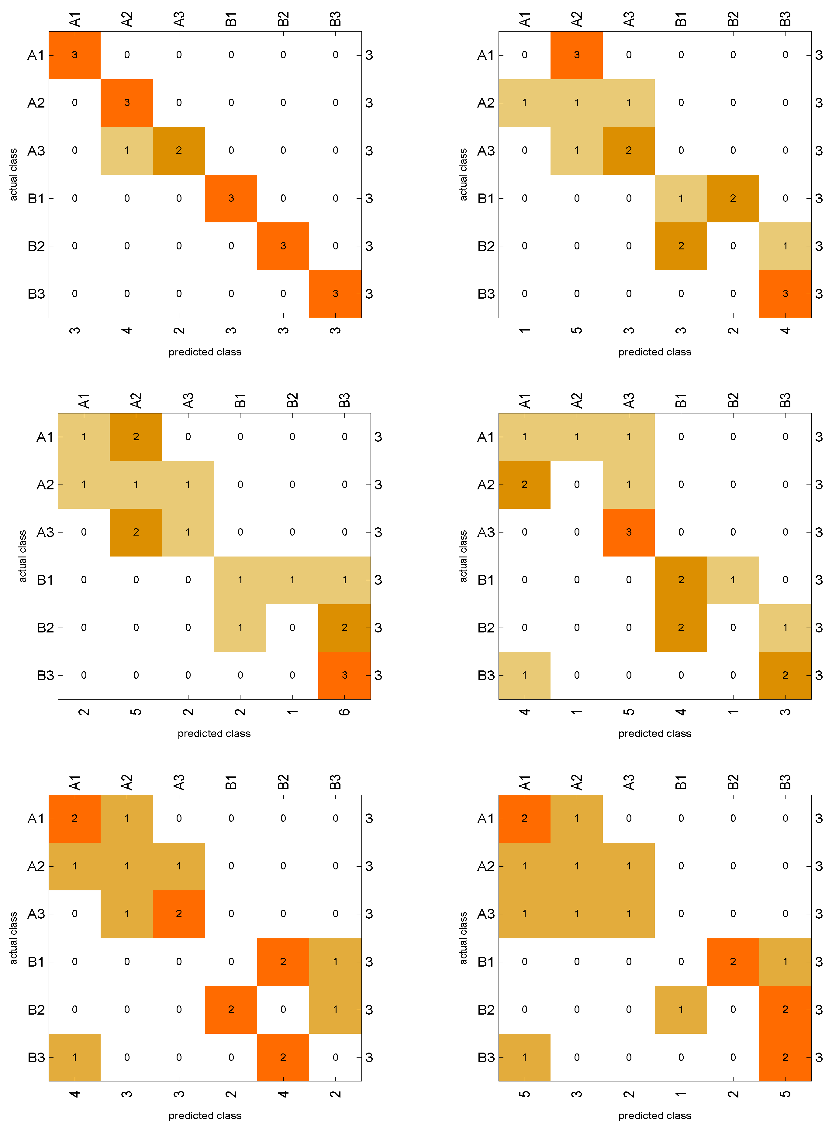
4. Quality of a Lending Portfolio

The financial institute can express the set of training, i.e., the template for sample assignment. The training data for AI are significant since, without such data, it is not possible to train a machine that could only read a pattern or understand an object from learning such data sets. As data are fed into the machine model with algorithms, The accuracy of model predictiOn grows.
Now to start the procedure, The technique of KNN is used to train the data and do the classification on the training set given as follows:
Training set = {{3., 50, 10} -> "A3", {5, 70, 19} -> "A3", {10, 85, 28} -> "A3",
        {3, 85, 32} -> "A2", {5, 145, 65} -> "A2", {10, 200, 89} -> "A2",
        {3, 120, 50} -> "A1", {5, 200, 92} -> "A1",
        {10, 260, 134} -> "A1", {3, 210, 125} -> "B3",
        {5, 300, 170} -> "B3", {10, 390, 190} -> "B3",
        {3, 290, 123} -> "B2", {5, 370, 201} -> "B2",
        {10, 440, 326} -> "B2", {3, 360, 124} -> "B1",
        {5, 470, 250} -> "B1", {10, 550, 320} -> "B1"};
In fact, The financial institution can define the training set. The numerical data considered here for the training set and the validity set are obtained from some banks.
Here, we leverage all the previously mentioned approaches to perform data classification using the KNN algorithm and compare their results against each other while the distribution smoothing parameter is set to 0.5 for all of them.
It is worth mentioning that all the three sub methods of the KNN, i.e., Scan, k-d tree, and Octree are implemented in this work and all produce similar outputs in our financial problems. However, we focus on Octree in our scenario rather than Scan and k-d tree, since our data set is three-dimensional. The results are then gathered into a classifier function which can be acted on various large data sets.
Remark 1.
The model here is finally saved as a classifier function, which can then be acted on any large set of unlabeled data as follows:Mathematics 09 00017 i001
It is now necessary to verify the reliability of the model obtaining from the KNN technique for different values of k before proceeding on large financial data sets. To be more precise, once the entire training set has been propagated through the model, then the model is tested on a validity set (development set). If the error over the entire validity set is reasonable, then one may rely on the model for prediction and also when real-time updates could occur in the portfolio. Here, The validity set is given as follows:
Validity set = {{3, 46, 38} -> "A3", {5, 81, 29} -> "A3", {10, 92, 38} -> "A3",
        {3, 91, 19} -> "A2", {5, 155, 42} -> "A2", {10, 202, 69} -> "A2",
        {3, 126, 27} -> "A1", {5, 215, 55} -> "A1",
        {10, 259, 102} -> "A1", {3, 219, 90} -> "B3",
        {5, 311, 123} -> "B3", {10, 399, 166} -> "B3",
        {3, 292, 85} -> "B2", {5, 378, 200} -> "B2",
        {10, 442, 302} -> "B2", {3, 350, 145} -> "B1",
        {5, 460, 203} -> "B1", {10, 568, 326} -> "B1"};
In our case, since the training and testing data-sets are small, cross validation is not performed, but rather the data points are chosen carefully to be representative of the unseen data. after cherry picking the training and testing data points, The model is trained and tested, after which the accuracy for different learning methods is reported.
Normally, in ML, we use the validity set to tune our model parameters and a test set to assess the out-of-sample model performance. Apart from that, we employ this to compare the behavior of different techniques at this stage and pick up the best one. To compare the results of the classification problem in terms of statistical measurements, a confusion matrix (a.k.a., The error matrix [37]) is taken into account for comparisons. This matrix is a specific matrix/table layout that gives us visualization of the algorithm’s performance for a supervised learning one. Each row of the matrix shows the instances in a predicted class while each column represents the instances in an actual class (or vice versa).
In addition, The F measure, which is also known as F-score or F 1 -score, is also provided for different choices of the free parameter k in Table 1 to reveal, for what values of this parameter, we may get the best performance of the nearest neighbors supervised classifier. The F 1 -score is a measure of a test’s accuracy. It considers both the precision p and the recall r of the test to compute the score when r is the number of correct positive results divided by the number of all relevant samples as follows [38]:
F 1 = 2 p r p + r ,
wherein p is the number of correct positive results divided by the number of all positive results returned by The classifier.
Six different values for k are considered, and the results are reported on the validity set in Table 1. The measurement of the classifier for k = 1 yields the identification of the six labels. in fact, The choice of k = 1 yields the best performance in terms of such financial data and could be considered for imposing on large data.
The accuracy of different forms of this classifier and the confusion matrices in Figure 1 show that the best accuracy belongs to the k = 1 case.
Remark 2.
Noting that the nonstandard discriminant classifiers such as SVM (which separates the training data into two classes using a maximum-margin hyperplane), RF (which uses an ensemble of decision trees to predict the class) and ANN (which is composed of layers of artificial neuron units) perform poorly for doing the classifications of such type of financial data as can be seen from their confusion matrices in Figure 2. The plot of their matrices is not diagonal-like. The accuracy of RF, SVM, and ANN classifiers on the validity set are 0%, 50%, and 33%, respectively, which indicate that these classifiers are not useful for the aim of this work. Further details about the comparisons are brought forward in Table 2.

4.1. Variable Importance
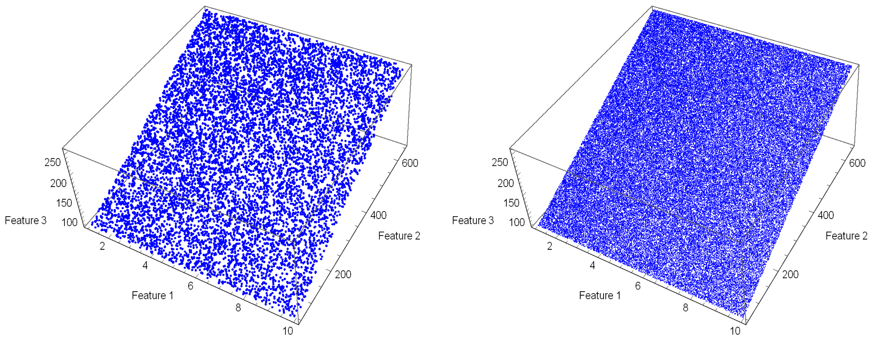
Variable importance by classifiers is another point that must be discussed based on the action of the model on the test set. Here, we summarize these results in Table 3 with the ratios based on the baseline accuracy. The idea is that, if the number of variables (attributes) is l for each i, 1 i l , then shuffle the values of the i-th column of the test data and find the classification success rates. In addition, finally, compare the obtained l classification success rates between each other and with the success rates obtained by the un-shuffled test data [39]. Noting that the variables for which the classification success rates are the worst are the most decisive (a mean of over 20 shuffles is considered). Results reveal that, for the main model based on KNN ( k = 1 ) and also the other techniques, The second feature has the most important importance.

4.2. Data

Now, the main data set is used for the classification of the lending portfolio. Hence, three different simulated data sets are considered and compared here. The data sets can be reproduced in the programming package Mathematica as follows:
SeedRandom[1]
data2 = Table[
   Drop[
    {a = RandomInteger[{50, 650}],
     RandomReal[{1, 10}], a, IntegerPart[a/3] + 50}
    , 1]
   , {10,000}];
Figure 3 shows a sample set of data for two cases of the sizes 10,000 and 100,000. Here, three sets are considered of the sizes 10,000, 50,000, and 100,000. Clearly, the larger the data set, The more elapsed time required for classifications. We have also chosen SeedRandom [ 1 ] intentionally to let the reader reproduce the data set and perform the classifiers to get the same results of this work.
The computational workouts are done here using the programming package Mathematica 12.0 [40] and Windows 10, Core i7-9750H CPU on MSI Laptop with 16 GB of RAM on SSD memory having six kernels for parallel computations.

4.3. General Observations

The results of classifications are provided in Figure 4 revealing that the largest proportion of loans falls into a B1 rating category and the smallest to the A3 category, which is naturally expected based on the organization of the training set coming from The banks.
The large data sets considered for verifying the proposed model have maturities which could be any integer number in the interval [ 1 ,   10 ] here.
Technically speaking, since the procedure of classification using the ML techniques on the list of large data sets is in fact imposing a classifier function on the list’s items, thus the procedure can significantly be speeded up by incorporating parallel techniques. Now, we compare the non-parallelization way to the parallelization results in terms of time (in second) in Figure 5 for two parallelization approaches of Coarsest Grained and Finest Grained. We applied the built-in Mathematica commands for doing this purpose.
In the finest grained method, The program is divided into large number of smaller, less computationally heavy tasks to be processed on individual processors, whereas, in coarsest grain, The program is divided into several large tasks to be processed [41]. in both methods, there is always a trade-off between the computation and communication times as if in the case of such computationally heavy tasks and easy tasks, The computation time and communication time would be the bottlenecks, respectively.
As shown in Figure 5, The coarsest grained approach for parallelization gives the best results in contrast to its competitor Finest Grained, indicating that the task of classifying such financial data is best to be segregated into several large tasks in order to alleviate the effect of communicatiOn time.

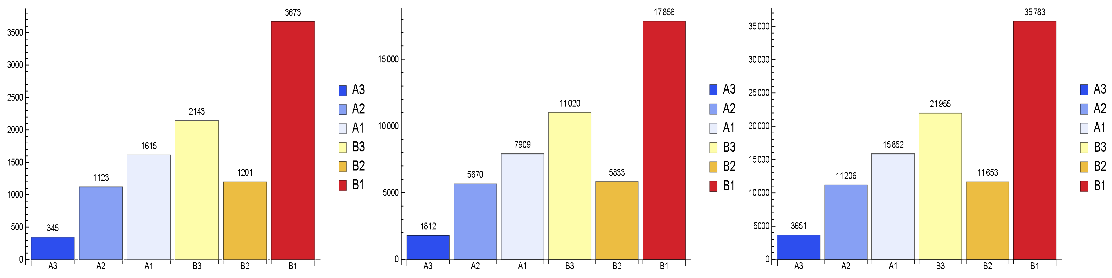
4.4. Dynamic Update of The Portfolio

The set-up classifier can also work with dynamically-changing portfolios. We can add, for instance, 100 new loans to the existing portfolio and to check how quickly the classification with these newly added loans can be done. This is done here using the following piece of code:
SeedRandom[2]
number = 100;
newlyloans = Table[
   Drop[
    {a = RandomInteger[{50, 650}], RandomReal[{1, 10}],
     a, IntegerPart[a/3] + 50}
    , 1]
   , {number}];
The results for such an updated portfolio are furnished in Figure 6.

4.5. Experiments: Top Probabilities

Let us test the constructed ML model on several unlabeled experiments arising by changing the maturity, the credit spreads, and the remaining credits, in order to find the probabilities of the classes given the features of each example.
The results for this objective are given in Table 4 showing the top probabilities using the proposed model of KNN classifier with k = 1 . The sum of all probabilities is roughly one, and, when the maturity is not even an integer and the other features are varying, the probability for a loan for belonging in each ranking category can be observed easily.
The classification technique is fruitful in economic and financial data organization and dimensionality reduction in supervised ML. It is beneficial when a huge load of various data has to be organized into class structures or given certain associations with structural hierarchy. Accordingly, as it was observed, this is ideal for finding patterns in large data sets. Hence, supervised ML is useful for risk management.

5. Conclusions

We know that banks are considered as failures if the government/owner regulator forces them to shut down due to insolvency problems. Due to the strong interconnection between banks and their essential role in financing the economy, the failure of banks is dangerous for the economy in contrast to the failure of other business firms. Even in several situations, the bankruptcy of one bank can cause a knock-on effect, which can spread rapidly and have a negative impact on other banks (systemic risk). Such matters along with the process of handling large scale data coming from different types of banks or lending portfolios make it necessary to investigate new tools such as ML algorithms for classification and prediction.
In this paper, we have investigated the classification as the data-mining technique in recognition of patterns and ML under supervision. Comparison of this classification to several of the existing data exploration algorithms was furnished, and it was shown by the way of illustration how credit risk categorization can be easily obtained with classification techniques. This was demonstrated on the credit rating case where simple implementation led to an efficient approach that was able to classify large unlabeled portfolios with real-time updates. As the advantage of the proposed discussions, our model can be useful for bank managers to quickly manage the risk of giving loans to different candidates by allocating them in appropriate groups in terms of the maturity, the credit spread, and the remaining credit. The results upheld the discussions of [23] but with three features and can be investigated for similar purposes having more features. The disadvantage of this process is that of the KNN technique, which is a lazy learner. For future studies, one may investigate the application of clustering techniques as data-mining and data-processing techniques for tackling large portfolios containing multi assets and grouping them into simple representative objects. This could be pursued on financial data having unique financial returns.

Author Contributions

Conceptualization, F.S. and H.M.; methodology, F.S.; software, F.S. and H.M.; validation, F.S., H.M. and S.S.; formal analysis, F.S. and H.M.; investigation, F.S. and H.M.; writing—original draft preparation, F.S., H.M. and S.S.; writing—review and editing, F.S., H.M. and S.S.; visualization, F.S., H.M. and S.S.; supervision, F.S.; funding acquisition, S.S. All authors have read and agreed to the published version of the manuscript.

Funding

The APC was funded by Stanford Shateyi from University of Venda.

Data Availability Statement

We state that all data used here are simulated using the Wolfram Mathematica Software https://www.wolfram.com, and the associated pieces of code can be observed in the text.

Acknowledgments

The authors would like to thank all four referees for many suggestions and corrections on an earlier version of this paper which helped improve the work.

Conflicts of Interest

The authors declare that they have no known competing financial interests or personal relationships that could have appeared to influence the work reported in this paper.

References

  1. De Prado, M.L. Advances in Financial Machine Learning; Wiley: Hoboken, NJ, USA, 2018. [Google Scholar]
  2. Bishop, C.M. Pattern Recognition and Machine Learning; Springer: Singapore, 2020; Volume 28, pp. 1639–1670. [Google Scholar]
  3. Nazemi, A.; Heidenreich, K.; Fabozzi, F.J. Improving corporate bond recovery rate prediction using multi-factor support vector regressions. Eur. J. Oper. Res. 2018, 271, 664–675. [Google Scholar] [CrossRef]
  4. Pławiak, P.; Abdar, M.; Rajendra Acharya, U. Application of new deep genetic cascade ensemble of SVM classifiers to predict the Australian credit scoring. Appl. Soft Comput. J. 2019, 84, 105–740. [Google Scholar] [CrossRef]
  5. Tan, Z.; Yan, Z.; Zhu, G. Stock selection with random forest: An exploitation of excess return in the Chinese stock market. Heliyon 2019, 5, e02310. [Google Scholar] [CrossRef] [PubMed] [Green Version]
  6. Gupta, R.; Pierdzioch, C.; Vivian, A.J.; Wohar, M.E. The predictive value of inequality measures for stock returns: An analysis of long-span UK data using quantile random forests. Financ. Res. Lett. 2019, 29, 315–322. [Google Scholar] [CrossRef] [Green Version]
  7. Abdar, M.; Wijayaningrum, V.N.; Hussain, S.; Alizadehsani, R.; Pławiak, P.; Acharya, U.R.; Makarenkov, V. IAPSO-AIRS A novel improved machine learning-based system for wart disease treatment. J. Med. Syst. 2019, 220, 43. [Google Scholar] [CrossRef]
  8. Tuncer, T.; Ertam, F.; Dogan, S.; Aydemir, E.; Pławiak, P. Ensemble residual network-based gender and activity recognition method with signals. J. Supercomput. 2020, 76, 2119–2138. [Google Scholar] [CrossRef]
  9. Kandala, R.N.V.P.S.; Dhuli, R.; Pławiak, P.; Naik, G.R.; Moeinzadeh, H.; Gargiulo, G.D.; Gunnam, S. Towards real-time heartbeat classification: Evaluation of nonlinear morphological features and voting method. Sensors 2019, 19, 5079. [Google Scholar] [CrossRef] [PubMed] [Green Version]
  10. Henrique, B.M.; Sobreiro, V.A.; Kimura, H. Literature review: Machine learning techniques applied to financial market prediction. Expert Syst. Appl. 2019, 124, 226–251. [Google Scholar] [CrossRef]
  11. Weinan, E. Machine learning and computational mathematics. Commun. Comput. Phys. 2020, 28, 1639–1670. [Google Scholar]
  12. Le, H.H.; Viviani, J.-L. Predicting bank failure: An improvement by implementing a machine-learning approach to classical financial ratios. Res. Int. Busin. Financ. 2018, 44, 16–25. [Google Scholar] [CrossRef]
  13. Altman, E.I. Financial ratios, discriminant analysis and the prediction of corporate bankruptcy. J. Financ. 1968, 23, 589–609. [Google Scholar] [CrossRef]
  14. Owusu-Ansah, E.D.-G.J.; Barnes, B.; Donkoh, E.K.; Appau, J.; Effah, B.; Nartey, M.M. Quantifying economic risk: An application of extreme value theory for measuring fire outbreaks financial loss. Financ. Math. Appl. 2019, 4, 1–12. [Google Scholar]
  15. Carbo-Valverde, S.; Cuadros-Solas, P.; Rodríguez-Fernández, F. A machine learning approach to the digitalization of bank customers: Evidence from random and causal forests. PLoS ONE 2020, 15, e0240362. [Google Scholar] [CrossRef] [PubMed]
  16. Cuadros-Solas, P.J.; Salvador Muñoz, C. Potential spillovers from the banking sector to sovereign credit ratings. Appl. Econ. Lett. 2020. [Google Scholar] [CrossRef]
  17. Khandani, A.E.; Kim, A.J.; Lo, A.W. Consumer credit-risk models via machine-learning algorithms. J. Bank. Financ. 2010, 34, 2767–2787. [Google Scholar] [CrossRef] [Green Version]
  18. De Moor, L.; Luitel, P.; Sercu, P.; Vanpee, R. Subjectivity in Sovereign credit ratings. J. Bank. Financ. 2010, 88, 366–392. [Google Scholar] [CrossRef]
  19. Klaas, J. Machine Learning for Finance; Packt Publishing: Birmingham, UK, 2019. [Google Scholar]
  20. Eller, P.R.; Cheng, J.-R.C.; Maier, R.S. Dynamic linear solver selection for transient simulations using multi-label classifiers. Procedia Comput. Sci. 2012, 9, 1523–1532. [Google Scholar] [CrossRef]
  21. Kim, H.; Cho, H.; Ryu, D. Corporate default predictions using machine learning: Literature review. Sustainability 2020, 12, 6325. [Google Scholar] [CrossRef]
  22. Hammad, M.; Pławiak, P.; Wang, K.; Rajendra Acharya, U. ResNet-Attention model for human authentication using ECG signals. Expert Syst. 2020, e12547. [Google Scholar] [CrossRef]
  23. Hlivka, I. Machine Learning in Finance: Data Classification Approach; Quant Solutions Group: London, UK, 2015. [Google Scholar]
  24. Sirignano, J.; Sadhwani, A.; Giesecke, K. Deep learning for mortgage risk. J. Financ. Econom. 2020, 1–20. [Google Scholar] [CrossRef] [Green Version]
  25. Yu, Q.; Miche, Y.; Séverin, E.; Lendasse, A. Bankruptcy prediction using extreme learning machine and financial expertise. Neurocomputing 2014, 128, 296–302. [Google Scholar] [CrossRef]
  26. Galindo, J.; Tamayo, P. Credit risk assessment using statistical and machine learning basic methodology and risk modeling applications. Comput. Econ. 2000, 15, 107–143. [Google Scholar] [CrossRef]
  27. Son, Y.; Byun, H.; Lee, J. Nonparametric machine learning models for predicting the credit default swaps: An empirical study. Expert Sys. Appl. 2016, 58, 210–220. [Google Scholar] [CrossRef]
  28. Jaafar, H.B.; Mukahar, N.B.; Ramli, D.A.B. A methodology of nearest neighbor: Design and comparison of biometric image database. In Proceedings of the 2016 IEEE Student Conference on Research and Development (SCOReD), Kuala Lumpur, Malaysia, 13–14 December 2016; pp. 1–6. [Google Scholar]
  29. Döring, M.; Györfi, L.; Walk, H. Rate of convergence of k-nearest-neighbor classification rule. J. Mach. Lear. Res. 2018, 18, 1–16. [Google Scholar]
  30. Elseberg, J.; Magnenat, S.; Siegwart, R.; Nüchter, A. Comparison on nearest-neigbour-search strategies and implementations for efficient shape registration. J. Soft. Eng. Robot. 2012, 3, 2–12. [Google Scholar]
  31. Gan, G.; Ma, C.; Wu, J. Data Clustering: Theory, Algorithms, and Applications; SIAM: Philadelphia, PA, USA, 2007. [Google Scholar]
  32. Teknomo, K. K-Nearest Neighbor Tutorial. 2019. Available online: https://people.revoledu.com/kardi/tutorial/KNN/ (accessed on 16 November 2020).
  33. Vieira, J.R.D.C.; Barboza, F.; Sobreiro, V.A.; Kimura, H. Machine learning models for credit analysis improvements: Predicting low-income families’ default. Appl. Soft Comput. 2019, 83, 105640. [Google Scholar] [CrossRef]
  34. Moayedi, H.; Bui, D.T.; Kalantar, B.; Foong, L.K. Machine-learning-based classification approaches toward recognizing slope stability failure. Appl. Sci. 2019, 9, 4638. [Google Scholar] [CrossRef] [Green Version]
  35. Wu, D.; Fang, M.; Wang, Q. An empirical study of bank stress testing for auto loans. J. Financ. Stab. 2018, 39, 79–89. [Google Scholar] [CrossRef]
  36. Cremers, K.J.M.; Driessen, J.; Maenhout, P. Explaining the level of credit spreads: Option-implied jump risk premia in a firm value model. Rev. Financ. Stud. 2008, 21, 2209–2242. [Google Scholar] [CrossRef] [Green Version]
  37. Stehman, S.V. Selecting and interpreting measures of thematic classification accuracy. Remote Sens. Environ. 1997, 62, 77–89. [Google Scholar] [CrossRef]
  38. Chinchor, N. MUC-4 Evaluation Metrics. Proceeding of the Fourth Message Understanding Conference, McLean, Virginia, 16–18 June 1992; pp. 22–29. [Google Scholar]
  39. Antonov, A. Variable Importance Determination by Classifiers Implementation in Mathematica; Lecture Notes; Wolfram: Windermere, FL, USA, 2015. [Google Scholar]
  40. Georgakopoulos, N.L. Illustrating Finance Policy with Mathematica; Springer International Publishing: Cham, Switzerland, 2018. [Google Scholar]
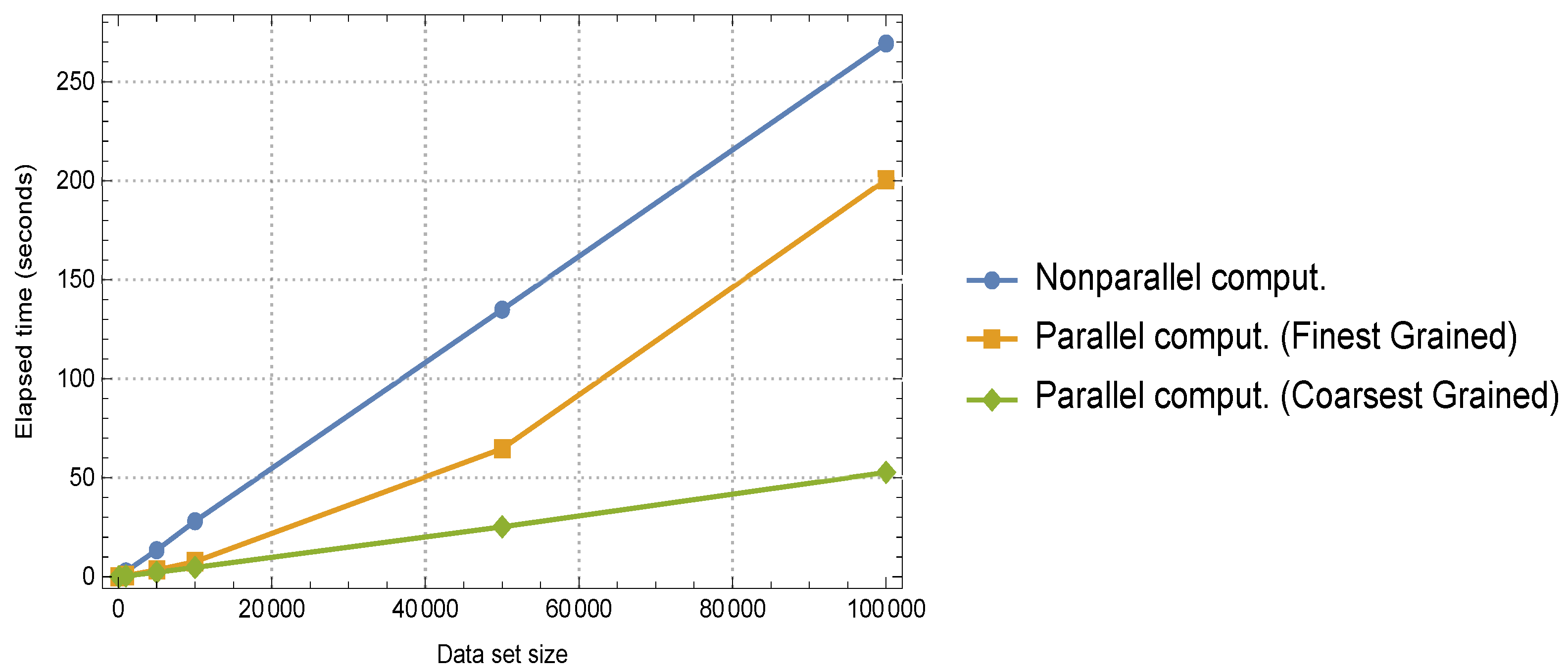
  41. Kwiatkowski, J. Evaluation of parallel programs by measurement of its granularity. Parallel Process. Appl. Math. 2002, 2328, 145–153. [Google Scholar]
Figure 1. The confusion matrices for the results of classification based on KNN, when k = 1 , k = 2 , k = 3 , k = 4 , k = 5 , and k = 6 are in (top-left), (top-right), (middle-left), (middle-right), (bottom-left), and (bottom-right), respectively.
Mathematics 09 00017 g001
Figure 2. The confusion matrices for the results of classification based on RF (left), SVM (center), and ANN (right).
Mathematics 09 00017 g002
Figure 3. The lending portfolio having different sizes, (left) for 10,000 and (right) for 100,000.
Mathematics 09 00017 g003
Figure 4. Classification of (Left): when the size is 10,000. (Center): when the size is 50,000. (Right): when the size is 100,000.
Mathematics 09 00017 g004
Figure 5. Time comparison for the classification by increasing the size of the lending portfolio in the absence and presence of parallelization.
Mathematics 09 00017 g005
Figure 6. Classification of the lending portfolio with 100 new assets added. (Left): when the size is 10,000. (Center): when the size is 50,000. (Right): when the size is 100,000.
Mathematics 09 00017 g006
Table 1. The results of F-scores for the validity set under different values of k.
A1A2A3B1B2B3Accuracy
k = 1 1.000.850.801.001.001.0094%
k = 2 0.000.250.660.330.000.8538%
k = 3 0.400.250.400.400.000.6638%
k = 4 0.280.000.750.570.000.6644%
k = 5 0.570.330.660.000.000.0027%
k = 6 0.500.330.400.000.000.5033%
Table 2. The compared classifiers information.
KNNRFSVMANN
Sub-methodOctree,
Neighbors number = 1
Feature fraction = 0.57,
Leaf size = 3,
Tree number = 50
Kernel type =
Radial basis function,
Gamma scaling parameter = 0.34,
Multi class strategy
= one vs. one
Network depth = 8,
Max. training
rounds = 1000
Single evaluation time1.45 ms/example3.77 ms/example9.57 ms/example2.79 ms/example
Batch evaluation speed144. example/ms44.4 example/ms9.09 example/ms53.4 example/ms
Loss 2.10 ± 0.54 1.80 ± 0.13 1.67 ± 0.28 1.33 ± 0.60
Model memory115 kB198 kB212 kB358 kB
Training time208 ms224 ms819 ms2.46 s
Table 3. Variable importance comparisons with different classifiers.
Techniques→KNN ( k = 1 ) SVM ANN
FeaturesShuffled AccuracyRatioShuffled AccuracyRatioShuffled AccuracyRatio
Maturity0.510.540.330.670.361.10
Credit spread0.220.240.210.420.150.47
Remaining credit0.440.470.330.670.401.21
Table 4. Probabilities of belonging to each ranking categories by varying the three features under the discussed ML model.
MaturityCredit SpreadRemaining Credit P ( A 1 ) P ( A 2 ) P ( A 3 ) P ( B 1 ) P ( B 2 ) P ( B 3 )
2.5100250.0550.0550.7220.0550.0550.055
2.5100500.0550.7220.0550.0550.0550.055
2.5100750.0550.7220.0550.0550.0550.055
2.51001000.0550.7220.0550.0550.0550.055
2.5200250.0550.7220.0550.0550.0550.055
2.5200500.0550.7220.0550.0550.0550.055
2.5200750.7220.0550.0550.0550.0550.055
2.52001000.7220.0550.0550.0550.0550.055
2.5300250.7220.0550.0550.0550.0550.055
2.5300500.7220.0550.0550.0550.0550.055
2.5300750.7220.0550.0550.0550.0550.055
2.53001000.7220.0550.0550.0550.0550.055
2.5400250.7220.0550.0550.0550.0550.055
2.5400500.0550.0550.0550.0550.0550.722
2.5400750.0550.0550.0550.0550.0550.722
2.54001000.0550.0550.0550.0550.0550.722
2.5500250.0550.0550.0550.7220.0550.055
2.5500500.0550.0550.0550.0550.7220.055
2.5500750.0550.0550.0550.0550.7220.055
2.55001000.0550.0550.0550.0550.7220.055
5.100250.0550.0550.7220.0550.0550.055
5.100500.0550.7220.0550.0550.0550.055
5.100750.0550.7220.0550.0550.0550.055
5.1001000.0550.7220.0550.0550.0550.055
5.200250.0550.7220.0550.0550.0550.055
5.200500.0550.7220.0550.0550.0550.055
5.200750.7220.0550.0550.0550.0550.055
5.2001000.7220.0550.0550.0550.0550.055
5.300250.7220.0550.0550.0550.0550.055
5.300500.7220.0550.0550.0550.0550.055
5.300750.7220.0550.0550.0550.0550.055
5.3001000.7220.0550.0550.0550.0550.055
5.400250.7220.0550.0550.0550.0550.055
5.400500.0550.0550.0550.0550.0550.722
5.400750.0550.0550.0550.0550.0550.722
5.4001000.0550.0550.0550.0550.0550.722
5.500250.0550.0550.0550.7220.0550.055
5.500500.0550.0550.0550.0550.7220.055
5.500750.0550.0550.0550.0550.7220.055
5.5001000.0550.0550.0550.0550.7220.055
7.5100250.0550.0550.7220.0550.0550.055
7.5100500.0550.7220.0550.0550.0550.055
7.5100750.0550.7220.0550.0550.0550.055
7.51001000.0550.7220.0550.0550.0550.055
7.5200250.0550.7220.0550.0550.0550.055
7.5200500.0550.7220.0550.0550.0550.055
7.5200750.7220.0550.0550.0550.0550.055
7.52001000.7220.0550.0550.0550.0550.055
7.5300250.7220.0550.0550.0550.0550.055
7.5300500.7220.0550.0550.0550.0550.055
7.5300750.7220.0550.0550.0550.0550.055
7.53001000.7220.0550.0550.0550.0550.055
7.5400250.7220.0550.0550.0550.0550.055
7.5400500.0550.0550.0550.0550.0550.722
7.5400750.0550.0550.0550.0550.0550.722
7.54001000.0550.0550.0550.0550.0550.722
10.100250.0550.0550.7220.0550.0550.055
10.100500.0550.7220.0550.0550.0550.055
10.100750.0550.7220.0550.0550.0550.055
10.1001000.0550.7220.0550.0550.0550.055
Publisher’s Note: MDPI stays neutral with regard to jurisdictional claims in published maps and institutional affiliations.

