Abstract
In this paper, we discuss a new stochastic diffusion process in which the trend function is proportional to the Lomax density function. This distribution arises naturally in the studies of the frequency of extremely rare events. We first consider the probabilistic characteristics of the proposed model, including its analytic expression as the unique solution to a stochastic differential equation, the transition probability density function together with the conditional and unconditional trend functions. Then, we present a method to address the problem of parameter estimation using maximum likelihood with discrete sampling. This estimation requires the solution of a non-linear equation, which is achieved via the simulated annealing method. Finally, we apply the proposed model to a real-world example concerning adolescent fertility rate in Morocco.
1. Introduction
Stochastic diffusion models are used to analyze the evolution of phenomena in multiple fields of science, including biology, finance, energy consumption and physics. In addition to traditional applications, stochastic diffusion processes (SDPs) have attracted considerable attention as analytical tools in areas such as cell growth, population growth and environmental studies. In this respect, see for example: Lognormal [1]; Gompertz [2]; Logistic [3]; Hyperbolic [4]; Rayleigh [5]; Pearson [6]; Weibull [7] and Brennan–Schwartz [8].
However in most of these studies, the processes considered are time homogeneous, in other words, the present state of the process depend only on the previous states and not on time. In contrast observations from many fields such a as neuroscience, finance and biology, suggest otherwise. Various non-homogeneous SDPs have been proposed to reflect this time dependent behavior, see for example: Lognormal [9], Gompertz [10], Vasicek [11], Brennan–Schwartz [12], and Gamma [13] processes.
In most of the aforementioned studies, the statistical inference is based on the maximum likelihood function, which is the product of transition densities. However, in some cases the closed form of the transition density is unknown, or has complicated expression, so the maximum likelihood method remains difficult to implement. Therefore many methods based on an approximation of the maximum likelihood were developed, such as: Prakasa-Rao [14], Kloeden et al. [15], Bibby et al. [16] and among others.
The Pareto type (II) distribution or Pearon type (IV) distribution, also called Lomax distribution, was introduced and studied by Lomax [17]. This distribution is commonly used in reliability and many lifetime testing studies. It is also used to analyze business data.
The density function of a Lomax distribution on with (scale parameter), and (shape parameter) is given by:
This distribution is a special case of a more general one called the Generalized Pareto distribution, the density function of which has the following form:
where and k are real parameters and . This distribution encompasses the Pareto distribution as a special case since if we set and we obtain the Equation (1).
In the present paper, we introduce a new Stochastic Lomax Diffusion Process (SLDP) as a non-homogeneous extension of the lognormal process, and which presents a trend function that is proportional to the Lomax density function. Moreover, the term adopted for the model we study will be improved by stochastic calculus. In this work, we will present a detailed and complete study of the Lomax Model. To this end, we will proceed as follows: In Section 2, we define the model in terms of stochastic differential equation (SDE), we then give the analytical expression of the solution of the proposed model. After which, we determine the Transition Probability Density Function (TPDF) and the trend functions. In Section 3, we deal with the problem of parameter estimation using Maximum Likelihood (ML) in the basis of discrete sampling. In this case, the system of likelihood equations does not have an explicit solution, so as a result the ML estimators cannot be given in the closed form. Then, one possible way to solve this basic problem is the use of numerical methods. In Section 4, we propose the simulated annealing method approximating the ML estimator then we show the results of the simulation of the process in Section 5. Moreover, in Section 6, we illustrate the results obtained by this method by reference to real data, namely the adolescent fertility rate in Morocco. Finally, we summarize the main conclusions drawn from this work.
2. The Model and Its Characteristics
2.1. The Model
The proposed model is the one-dimensional non-homogeneous SDP taking values on and with drift and diffusion coefficients:
where , and are real parameters.
Alternatively, the process defined above can be considered as the unique solution to the following SDE:
where is the one-dimensional standard Wiener process and is fixed in .
2.2. Distribution of the Process
The SDE in Equation (3) has a unique solution (see Kloeden et al [15]). In order to obtain this solution, we consider the appropriate transformation , then, by means of Itô formula, the Equation (3) becomes:
The solution to which is:
For . Hence, we deduce the expression of the solution to SDE in Equation (3):
then follows a Lognormal distribution:
where is the Lognarmal distribution. As a result, the TPDF of this process is found to be:
2.3. Trend Functions
From the properties of the Lognormal distribution, the main characteristics of the process can be determined, in particular the r-th conditional moment of the process is given by:
Then, by considering the case where in the previous expression, the conditional trend function of the process is:
In addition, taking into account the initial condition , the trend function of the process is:
We note here that:
- Otherwise, in the absence of white noise (i.e., ) the solution to equation Equation (3) is which is proportional in this case to the Lomax density function [18], with shape parameter and scale parameter , which can be denoted .
3. Maximum Likelihood Estimation
We consider a discrete sample of n observations of the process which we denote here , let denotes the moments when the process was observed with moreover we set , and finally is the parameters vector.
We know that the likelihood function is the product of the densities functions:
The Log-likelihood is given by:
where .
We differentiate this function with respect to the elements of vector to obtain the following equations:
Equation (8) is a second-degree equation in , which admits two solutions (since the discriminant is ). Therefore, from the non-negative solution corresponding to , the estimator is given by:
By replacing by in Equation (7), the estimator of is satisfying the following non-linear equation:
On the other hand, substituting by in Equation (10),
Obviously, this is a set of non-linear equations whose solutions may be difficult to find. To address this problem we use numerical resolution methods.
4. Computational Aspects
In this paper we suggest the simulated annealing (SA) method for solving the equations Equations (11) and (12). Hereafter is the description of the method.
Simulated annealing is a stochastic optimisation algorithm, developed in 1983 by [19], which approaches the global optimum of a given cost function by means of a random search. The fundamental idea of the algorithm is inspired by the process of annealing of metals in metallurgy. At each step of the simulated annealing algorithm a new point is randomly generated, if the new point improves the cost function it is accepted, otherwise, it is accepted with a probability , where f is the cost function and T is the temperature. Accepting points tat don’t improve the cost function allows the algorithm to escape local optima. The main disadvantage of this method is that the adjustment of the parameters (initial temperature, minimum temperature, cooling process and stopping conditions ...) considerably affects the time required to reach the extremum.
5. Simulation
To illustrate the process described by Equation (3), let us consider an equidistant discretisation of the interval with for . Let () and assume a discretisation step where N denotes the size of the sample. A total of 25 trajectories of the process were simulated, with , and and .
The results of the simulation, together with the Estimated Trend Function (ETF) of the process, are illustrated in Figure 1.

Figure 1.
Simulated sample paths vs. the Estimated Trend Function (ETF) for , .
Using the simulated annealing method to solve Equations (11) and (12), we obtained the estimators , and of each trajectory, and then considered the mean values of the estimators given by , and .
The values obtained used this method are , and . We then calculated the mean value of the simulated paths at each time step, namely, , where is the sample path j, is the time step i and m is the number of simulated trajectories. We also obtained the estimated trend functions of the process using each method, the result are plotted in Figure 2.
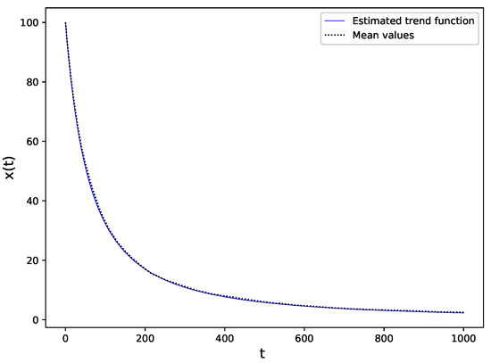
Figure 2.
ETFs vs. the mean values of simulated data.
6. Application
6.1. Data Description
In this application, we examined the variable defined by the adolescent fertility rate, which is the number of births per 1000 women aged 15 to 19, these data are annual and are available on the site: https://data.worldbank.org/. The average value for Morocco during the period from 1979 to 2018 is 42.395655 with a minimum value of 30.6810 in 2018 and a maximum value of 92.9376 in 1979. Table 1 illustrates the observed values, as well as the ETF and Estimated Conditional Trend Function (ECTF) during this period.

Table 1.
Table of adolescent fertility rate data by year.
In Figure 3, real data are plotted against trend functions (conditional and unconditional). The unconditional trend function provides a good estimates for the real values, the accuracy of those estimates can be more accurate if we consider the conditional trend function.
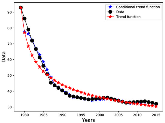
Figure 3.
Real data vs. trend function and conditional trend function.
Table 2 shows the estimated data for the years from 2016 to 2018 that were not used in the modeling and the actual data.
Table 2.
Forecasted values by year.
6.2. Goodness of Fit of the Model
The absolute mean error in percentage (MAPE) is the average of the deviations in absolute value compared to the observed values. It is a practical indicator of comparison, it makes it possible to evaluate the forecasts obtained from the models. We denote by , and n respectively the real values, the values predicted by the model and the number of predictions, so we have:
The symmetric mean percentage absolute error (SMAPE) is a measure of precision based on relative errors and is defined as follows:
The values obtained for the MAPE and SMAPE are: and , respectively. The MAPE value is less than 10, so according to Lewis [20] the values obtained by this model are “very precise”.
7. Conclusions
In this study of the stochastic Lomax diffusion process, from a theoretical point of view, we conclude that we can determine the basic probabilistic characteristics of the model and we obtain its parameter estimators. Using the maximum likelihood method in the basis of discrete sampling, we obtained a series of non linear equations which were solved by computational methods. We used the simulated annealing method to estimate the parameters of the model. Hence, a set of statistical results are obtained and show that the proposed process is enable to be applied to real data.
The Lomax model is applied to fit data for adolescent fertility rate in Morocco. The ETF presented a good description of the changing levels of the fertility rate. Furthermore, the period from 2016 to 2018 improved good forecasts. Then, the resulting values obtained by the MAPE and SMAPE were calculated and showed good results. Taking into account these points, we deduced that the methodology applied in the study of this new model was efficient and present a high degree of accuracy.
Author Contributions
Conceptualization, A.N., I.M. and R.G.S.; Data curation, A.N., I.M. and R.G.S.; Formal analysis, A.N., I.M. and R.G.S.; Funding acquisition, A.N. and R.G.S.; Investigation, A.N., I.M. and R.G.S.; Methodology, A.N., I.M. and R.G.S.; Project administration, A.N., I.M. and R.G.S.; Resources, A.N., I.M. and R.G.S.; Software, A.N., I.M. and R.G.S.; Supervision, A.N., I.M. and R.G.S.; Validation, A.N., I.M. and R.G.S.; Visualization, A.N., I.M. and R.G.S.; Writing–original draft, A.N., I.M. and R.G.S.; Writing–review–editing, A.N., I.M. and R.G.S. All authors have read and agreed to the published version of the manuscript.
Funding
This research was funded by “FEDER/Junta de Andalucía-Consejería de Economía y Conocimiento/ Proyecto A-FQM-228-UGR18”.
Institutional Review Board Statement
Not applicable.
Informed Consent Statement
Not applicable.
Data Availability Statement
Not applicable.
Acknowledgments
The authors are very grateful to Editor and referees for consecutive comments and suggestions. This research has been funded by “FEDER/Junta de Andalucía-Consejería de Economía y Conocimiento/ Proyecto A-FQM-228-UGR18”.
Conflicts of Interest
The authors declare no conflict of interest.
References
- Ramos-Ábalos, E.M.; Gutiérrez-Sánchez, R.; Nafidi, A. Powers of the Stochastic Gompertz and Lognormal Diffusion Processes, Statistical Inference and Simulation. Mathematics 2020, 8, 588. [Google Scholar]
- Gutiérrez, R.; Gutiérrez-Sánchez, R.; Nafidi, A. Modelling and forecasting vehicle stocks using the trends of stochastic Gompertz diffusion models: The case of Spain. Appl. Stoch. Model. Bus. Ind. 2009, 25, 385–405. [Google Scholar] [CrossRef]
- Giovanis, A.N.; Skiadas, C.H. A stochastic logistic innovation diffusion model studying the electricity consumption in Greece and the United States. Technol. Forecast. Soc. Chang. 1999, 61, 235–246. [Google Scholar] [CrossRef]
- Bibby, B.M.; Sørensen, M. A hyperbolic diffusion model for stock prices. Financ. Stoch. 1996, 1, 25–41. [Google Scholar] [CrossRef]
- Gutiérrez, R.; Gutiérrez-Sánchez, R.; Nafidi, A. The Stochastic Rayleigh diffusion model: Statistical inference and computational aspects. Applications to modelling of real cases. Appl. Math. Comput. 2006, 175, 628–644. [Google Scholar] [CrossRef]
- Forman, J.L.; Sørensen, M. The Pearson diffusions: A class of statistically tractable diffusion processes. Scand. J. Stat. 2008, 35, 438–465. [Google Scholar] [CrossRef]
- Nafidi, A.; Bahij, M.; Gutiérrez-Sánchez, R.; Achchab, B. Two-Parameter Stochastic Weibull Diffusion Model: Statistical Inference and Application to Real Modeling Example. Mathematics 2020, 8, 160. [Google Scholar] [CrossRef]
- Nafidi, A.; Moutabir, G.; Gutiérrez-Sánchez, R. Stochastic Brennan–Schwartz Diffusion Process: Statistical Computation and Application. Mathematics 2019, 7, 1062. [Google Scholar] [CrossRef]
- Gutiérrez, R.; Angulo, J.M.; González, A.; Pérez, R. Inference in lognormal multidimensional diffusion processes with exogenous factors: Application to modelling in economics. Appl. Stoch. Model. Data Anal. 1991, 7, 295–316. [Google Scholar] [CrossRef]
- Gutiérrez, R.; Gutiérrez-Sánchez, R.; Nafidi, A. Electricity consumption in Morocco: Stochastic Gompertz exogenous factors diffusion analysis. Appl. Energy 2006, 83, 1139–1151. [Google Scholar] [CrossRef]
- Gutiérrez, R.; Gutiérrez-Sánchez, R.; Nafidi, A.; Pascual, A. Detection, modelling and estimation of non-linear trends by using a non-homogeneous Vasicek stochastic diffusion. Application to CO2 emissions in Morocco. Stoch. Environ. Res. Risk Assess. 2012, 26, 533–543. [Google Scholar] [CrossRef]
- Picchini, U.; Ditlevsen, S.; De Gaetano, A. Maximum likelihood estimation of a time-inhomogeneous stochastic differential model of glucose dynamics. Math. Med. Biol. 2008, 25, 141–155. [Google Scholar] [CrossRef] [PubMed]
- Nafidi, A.; Gutiérrez, R.; Gutiérrez-Sánchez, R.; Ramos-Ábalos, E.; El Hachimi, S. Modelling and predicting electricity consumption in Spain using the stochastic Gamma diffusion process with exogenous factors. Energy 2016, 113, 309–318. [Google Scholar] [CrossRef]
- Prakasa Rao, B.L.S. Statistical Inference for Diffusion Type Processes; Arnold: London, UK, 1999. [Google Scholar]
- Kloeden, P.E.; Platen, E. Numerical Solution of Stochastic Differential Equations; Springer Science & Business Media: Berlin/Heidelberg, Germany, 2013; Volume 23. [Google Scholar]
- Bibby, B.M.; Sørensen, M. Martingale estimation functions for discretely observed diffusion processes. Bernoulli 1995, 17–39. [Google Scholar] [CrossRef]
- Lomax, K.S. Business failures: Another example of the analysis of failure data. J. Am. Stat. Assoc. 1954, 49, 847–852. [Google Scholar] [CrossRef]
- Meynial, E. Recueil Publié par la Faculté de Droit, à L’occasion de L’exposition Nationale Suisse de Genève; Editions Dalloz: Paris, France, 1898. [Google Scholar]
- Kirkpatrick, S.; Gelatt, C.D.; Vecchi, M.P. Optimization by simulated annealing. Science 1983, 220, 671–680. [Google Scholar] [CrossRef] [PubMed]
- Lewis, C.D. A Radical Guide to Exponential Smoothing and Curve Fitting; Butterworth-Heinemann: London, UK; Boston, MA, USA, 1982. [Google Scholar]
Publisher’s Note: MDPI stays neutral with regard to jurisdictional claims in published maps and institutional affiliations. |
© 2021 by the authors. Licensee MDPI, Basel, Switzerland. This article is an open access article distributed under the terms and conditions of the Creative Commons Attribution (CC BY) license (http://creativecommons.org/licenses/by/4.0/).