Optimal Disturbance Observer Design for High Tracking Performance in Motion Control Systems

Abstract

In this paper, a stability-driven optimal disturbance observer (DO) is proposed. The proposed method does not require any plant inverse dynamics to detect introduced disturbances or a stabilizing Q filter. It does not require additional compensators to resolve causality problems, due to the relative degree, or filters to solve instability problems of non-minimum phase plants. Using this method enables wideband and narrowband disturbances to be attenuated by simply multiplying the corresponding peak filters by the baseline weight function. Furthermore, the proposed DO guarantees the stability of closed-loop systems because the already designed outer-loop systems are considered as a target plant to be stabilized and because of the Lyapunov stability-based $H_{\infty }$ control. In the application example, it was confirmed that the proposed method is effective, and the position error signals were improved by 20.9% in commercial hard disk drives and 36.6% in optical image stabilization systems.

1. Introduction

One of the main causes of tracking performance degradation in the motion control systems is a disturbance. The disturbances act as additional input signals and generate unwanted output signals. In the steady-state, the unwanted output signals are added to a carefully designed output signal, resulting in distorting of the output signal. To reduce the effects of the disturbances, a disturbance observer (DO) has been used in many industrial applications [1].

Many motor control systems have employed DOs. In permanent-magnet synchronous motors, DOs have been used to remove generalized multiple disturbances, such as cogging torques, load torques, friction torques, measurement error effects, dead-time effects, and parameter perturbations [2]. To remove narrowband high-frequency disturbances, a discrete-time DO based on an infinite-impulse-response filter was proposed and applied to a permanent-magnet synchronous motor [3]. A robust high-order DO for the state-dependent Riccati-equation-based suboptimal speed controller of an interior permanent-magnet synchronous motor drive was proposed [4]. Unlike a conventional DO, in that study, the proposed high-order DO guarantees fast convergence of the estimated error. To reduce both noise and uncertainty, a modified DO was proposed, and the method was applied to brushless DC motor drive systems [5]. To obtain design flexibility, an algebraic-calculation-based DO was also proposed [6]. In two-axis control systems, DOs have also been used to enhance performance. A DO was applied to a double-gimbaled variable-speed control moment gyroscope. In the study, a DO was used to decouple the inner- and outer-gimbal system and to reject disturbances [7]. Star tracker systems also use DOs. A star tracker system based on a two-axis inertially stabilized platform, which was controlled by a DO, was also proposed for improving the stability accuracy [8]. Moreover, DOs have been utilized in flight control systems. A DO was used for consensus control [9], and the proposed method was applied to the formation control of unmanned aerial vehicles. The flight control of an unmanned aerial vehicle has high-order disturbances. To achieve the desired tracking performance, the disturbance is estimated by a DO based on Simpson’s approximation [10]. A novel second-order fixed-time sliding-mode control, based on a fixed-time sliding-mode DO for a small-scale unmanned helicopter, was developed for hovering in the presence of external disturbances [11]. A robust nonlinear DO was proposed for an integrated missile model with uncertainties and disturbances to estimate the uncertainties, disturbances, and state variables, including missile jerk [12]. DOs have also been applied to electric-circuit systems. In singularly perturbed systems with mismatched disturbances, the DO attenuates the mismatched disturbances [13]. In an AC power converter, a frequency-domain DO-based control was used to attenuate periodic uncertainties and disturbances [14]. In a DC–DC converter, the DO detected unmodeled effects, which were considered as lumped disturbance, and the disturbance was attenuated [15]. Two DOs were developed to deal with uncertainties and disturbances to improve velocity-tracking performance and to reduce energy consumption in an electrohydraulic actuator [16]. A DO was applied to an excavation [17]. In the study, an iterative learning control (ILC)-based DO was used to compensate for the difference between the ILC prediction and the true disturbance. Unlike in a conventional DO, a high-pass Q filter was used to estimate the disturbance for the electrohydraulic actuators [18].

A linear-matrix-inequality-based control has been widely utilized in different industrial applications, because the designed closed loop system is stable and the solution is optimal. The methodology comes from the fact that, because the intersection of the convex sets is a convex set as well, the global minimum can be found in the intersection. Therefore, if we can express design constraints in the form of the LMIs, we can find an optimal solution that satisfies all of those constraints. This is the first usage of the LMI approach, and it generally shows only time responses without frequency responses. As an another usage of the LMI approach, there is a loop shaper in the frequency domain, such as the $H_{\infty }$ control, and numerous studies have been conducted using these features. To achieve their unique goals, the researchers have suggested new cost functions to be minimized, even suggesting modified design frameworks. With their own design concepts, so far, many loop shaping methods based on $H_{\infty }$ control have been provided. In tele-micromanipulation system, an $H_{\infty }$-based loop shaping method was suggested [19]. In general, this loop shaping method has been used for motion control systems [20,21,22,23,24,25,26,27,28,29,30,31,32] including commercial Hard Disk Drives [33]. In addition, for DO design, this approach was used [34,35,36]. Here, note that, to achieve the special objects, the cost function, setup, must be carefully designed, and sometimes the design framework must be redesigned because the goal may not be achievable by using existing control blocks. In addition, because linear-matrix-inequality-based $H_{\infty }$ control can easily shape loop transfer functions [37,38,39], this method was used to modify existing loop functions [40,41]. It was also used to add additional stability margins to reduce a sensitivity peak [42] and to design a state space DO to maintain the advantages of state space controllers [43]. Recently, a Q filter design method to always stabilizes a DO was proposed [44]. However, the method still requires additional compensators because the method maintained a structure of the conventional DO.

A conventional DO estimates introduced disturbances using a plant inverse model and subtracted the estimated disturbance from total control effort. The conventional DO design procedure is as follows. First, a Q filter is designed to determine the bandwidth of the DO. Second, to solve the causality problem (strictly proper plant case), additional filters are designed. Third, if instability problems (non-minimum phase plant case) arise, then compensators based on all-pass filters should be designed. However, the conventional DO can only reduce the incoming disturbances at the same rate because only the bandwidth of the DO can be adjusted. In addition, although the three complicated design procedures were used, the stability was generally not guaranteed. A recent study [44] satisfied the stability to all types of models, but the method still required additional filters to solve the causality and instability problems.

In this study, a new unified design for the DO is proposed to remove the above three-step design procedure with guaranteed stability. For stability, the proposed design method uses a linear matrix inequality (LMI)-based $H_{\infty }$ control because the LMI-based control guarantees the stability of the closed loop systems. However, it is not simple to apply the DO design to the standard LMI framework because the closed loop systems are mixed with a plant, a conventional controller, and a DO. To apply the DO design to the LMI framework, in this study, the closed loop system with the DO is reinterpreted as a parallel system that consists of a plant, a conventional controller (C) forming outer-loop systems, and a DO ($C_{DO}^{conv}$) forming inner-loop systems. Because the DO can be written by $C_{DO}^{conv}=Q{P}_n^{-1}/(1-Q)$, the closed loop system with the DO can be considered as a plant controlled by the two parallel controllers, C and $C_{DO}^{conv}$. From the DO point of view, the DO controls a fictitious plant written by a function of the plant and the outer-loop controller C, that is, $f(P,C)$. In this study, an $f(P,C)$ is considered as a control target, which is a new design framework for DOs. Considering the function of the DO, the DO must be able to estimate the incoming disturbances well and remove the disturbance from the total control input. To reach the goal, a cost function to be minimized is defined by $z=|d-u_{DO}|$, where d and $u_{DO}$ are the incoming and estimated disturbances. Now, only one challenge of how and how much to eliminate the disturbance remains. In this study, the problem is solved by applying a weighting function that controls the capability of the disturbance rejection. With the proposed design framework and the suggested cost function, the generalized systems are augmented and finally the optimal DO is designed. Unlike previous studies, the type of the model needs not be considered in the proposed method. Therefore, additional filters and compensators to solve causality and instability problems caused by the model types are not required. The proposed method requires only one design specification—i.e., the frequency characteristics of the disturbances to be attenuated—and guarantees closed-loop system stability. This work makes the following contributions.

• The proposed method guarantees the stability of the closed-loop system because it provides optimal control based on the Lyapunov stability.
• It does not require plant inverse dynamics.
• Stabilizing Q filters are not required.
• The relative degree does not need to be considered. Therefore, additional filters to compensate for the relative degree are not necessary.
• Compensators based on all-pass filters are not required for non-minimum phase plants.
• Both wide and narrow band disturbances can be attenuated.
• Because this method provides more stability margins, it can reduce a sensitivity peak.

The rest of the paper is organized as follows. Section 2 contains the main research results. In this section, the conventional DO is discussed, and a new framework for optimal DO design is suggested. Section 3 includes the plant identification and controller design for stabilizing the outer loop. In addition, illustrative examples, including time and frequency responses, are presented. The conclusion follows.

2. Optimal Disturbance Observer Design

This section contains the main research results. The conventional DO is analyzed, and an optimal design framework is proposed. The formulation for the suggested method is also described.

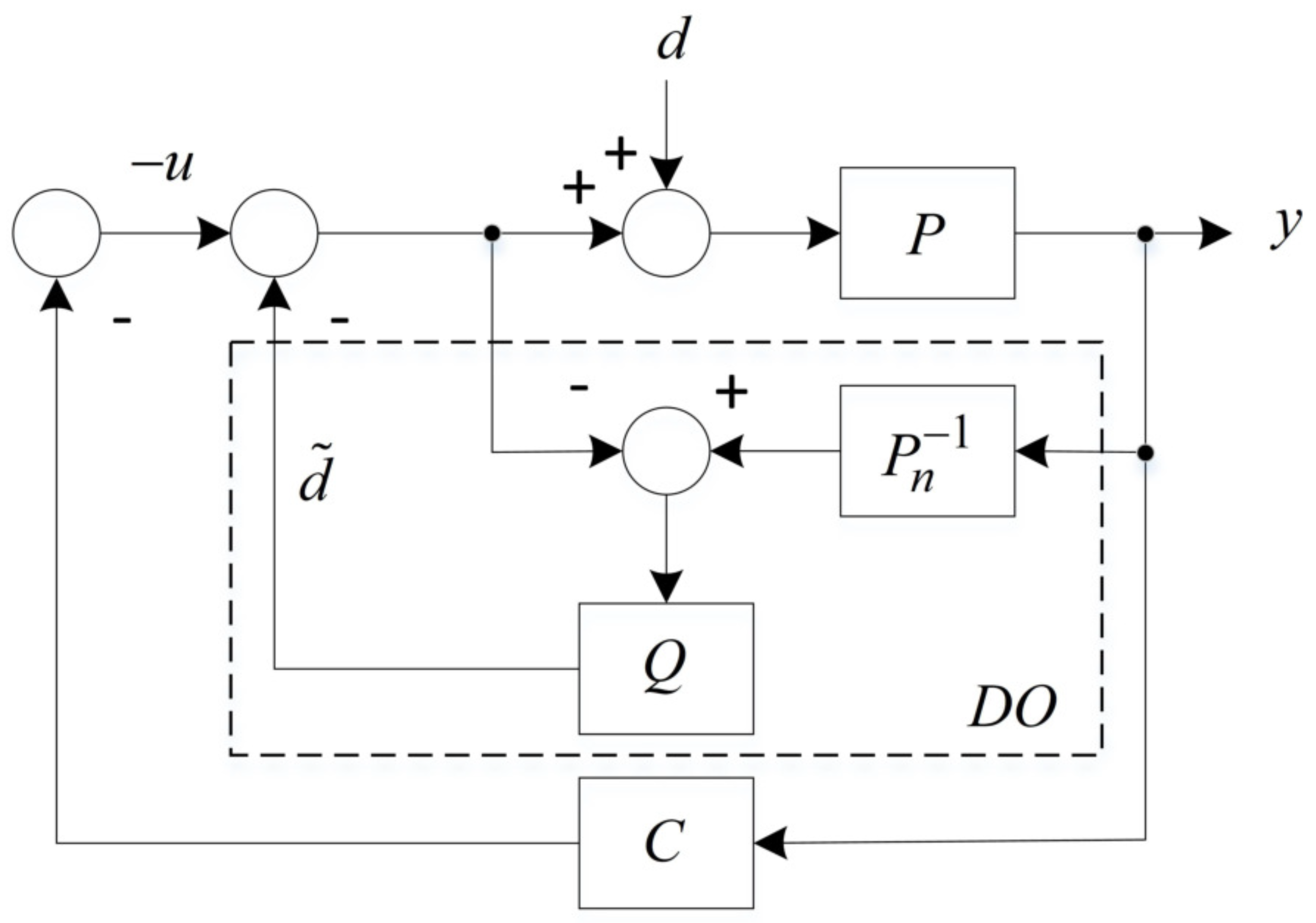
2.1. Conventional Disturbance Observer

In the presence of disturbances, DOs have been utilized intensively to reduce the disturbances. A DO monitor introduces disturbances and subtracts the disturbances from the total control effort. A typical DO is shown in Figure 1. In the figure, P is a plant to be controlled; $P_n$ is a nominal plant model; d is an external disturbance; C is a controller when there is no disturbance; Q is a low pass filter to stabilize DO when the disturbance is introduced.

If it is assumed that the output of the Q filter is not connected to the feedback loop, then the input of the Q filter, $i_Q$, can be calculated as

$$\begin{array}{c}\hfill \begin{array}{cc}\hfill i_Q& =u+P·P_n^{-1}(d-u)\hfill \\ \hfill & =u+P·P_n^{-1}d-P·P_n^{-1}u.\hfill \end{array}\end{array}$$

(1)

In the equation, if P and $P_n$ are identical, then $i_Q=d$. The role of the Q filter including additional compensators is to stabilize the DO, and to solve causality problems by relative degree and stability problems of the non-minimum phase plants. Finally, the estimated disturbance $\tilde{d}$ is applied to subtract d from the overall control input.

In Figure 1, the closed loop system can be rewritten by

$$\begin{array}{c}\hfill \begin{array}{cc}\hfill \frac{y\left(s\right)}{d\left(s\right)}& =\frac{P}{1+P\left(C+\frac{Q{P}_n^{-1}}{1-Q}\right)},\hfill \end{array}\end{array}$$

(2)

where $Q{P}_n^{-1}/(1-Q)$ is a transfer function of the DO, $C_{BO}^{conv}$. Therefore, the closed loop system is a parallel system controlled by two controllers C and $C_{BO}^{conv}$. From the DO point of view, the DO controls a composite plant defined by a function of P and C, that is, $f(P,C)$. Thus, the DO design problem is equivalent to design the DO to $f(P,C)$. In this study, because $f(P,C)$ is a pre-designed fictitious model in the absence of external disturbances, the optimal DO is designed to $f(P,C)$, which is a new DO design method.

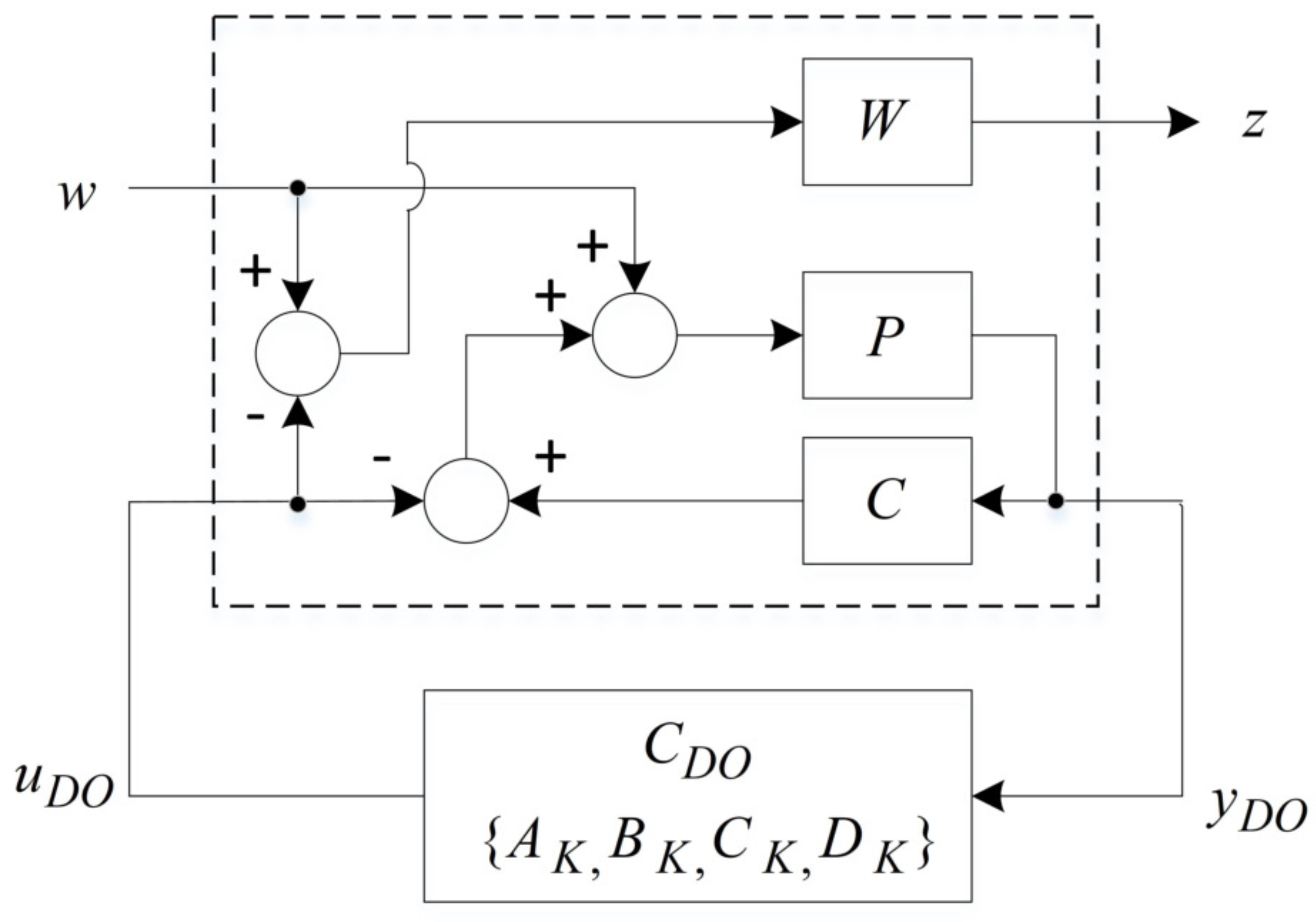
2.2. Design Framework for Optimal Disturbance Observer

With a given outer-loop controller, a DO should estimate introduced disturbances and subtract the disturbance from the control energy. To estimate the disturbance accurately, the output of the DO should be as close to d as possible in the frequency range of interest, which can be obtained by

$$\begin{array}{c}\hfill \begin{array}{c}\hfill \underset{\omega }{max}\left|d-u_{DO}\right|.\end{array}\end{array}$$

(3)

With this motivation, a new framework for optimal DO design is proposed, as shown in Figure 2. Using the block diagram, augmented systems are derived, and a linear-matrix-inequality-based DO is designed.

In the block diagram, W is a weight function to control the performance of the DO; w is an external disturbance; z is an output to be minimized; $C_{DO}$ is an optimal controller that minimizes a transfer function from w to z. In addition, $y_{DO}$ is a measurement, which is an input of the $C_{DO}$. $u_{DO}$ is an output of the $C_{DO}$, which is designed to be equivalent to w in the frequency range of interest. As for disturbances, there are wideband disturbances and narrowband disturbances. To attenuate each disturbance, we propose separated weighting functions, $W_{base}$ and $W_{peak}$, which are used to attenuate wideband disturbances and narrowband disturbances, respectively. $W_{base}$ for reducing wideband disturbance is represented by

$$\begin{array}{c}\hfill W_{base}\left(s\right)=\frac{{(s/M^{1/n}+{\omega }_B^{*})}^n}{(s+{\omega }_B^{*}{A}^{1/n}){)}^n}\end{array}$$

(4)

where M, A, ${\omega }_B^{*}$ and n are the upper bound, the lower bound, the bandwidth, and an order of $W_{base}\left(s\right)$, respectively [45]. Here, using $W_{base}$, wideband disturbances can be reduced. To reduce narrowband disturbances, a peak-filter-based weight function is used as

$$\begin{array}{c}\hfill W_{peak}\left(s\right)=\prod _{i=1}^N\frac{s^2+2{\zeta }_i{\omega }_{i}s+{\omega }_i^2}{s^2+2g_i{\zeta }_i{\omega }_{i}s+{\omega }_i^2}\end{array}$$

(5)

where ${\zeta }_i$ determines the width of the peak; ${\omega }_i$ is a peak frequency; $g_i$ is the magnitude of the peak response; N is the number of the narrow band disturbances [46]. In Equation (5), if we would like to reduce one narrow disturbance, then one second order filter should be designed. If we would like to reduce N narrow band disturbances, then $2\times N$ ordered filters should be designed. Therefore, the single second order filter reduces one narrow band disturbance. Finally, to reduce both wide and narrow band disturbances, two weight functions are combined as

$$\begin{array}{c}\hfill W\left(s\right)=W_{base}{W}_{peak},\end{array}$$

(6)

and their typical frequency responses are illustrated in Figure 3.

In the figure, the gain of $W_{base}^{-1}{W}_{peak}^{-}1$ is −14 dB at 1 Hz, which means that if an external disturbance (w) with the 1 Hz frequency component is introduced, the designed DO generates $u_{DO}$ that satisfies $|w-u_{DO}|={10}^{-14/20}$. This means that wide band disturbances that exist in the region below 10 Hz are reduced by approximately ${10}^{-14/20}$. At 50 Hz, the gain of $W_{base}^{-1}{W}_{peak}^{-}1$ is −20 dB, which implies that the introduced disturbance can be attenuated by −20 dB. In this sample weight, even though a single narrowband disturbance is considered, multiple narrowband disturbances could be considered with $N>1$ in Equation (5). However, if excessive high-order filters are used to reduce the multiple narrow band disturbances, the proposed design framework decreases the performance of the disturbance rejection to maintain stability. Therefore, critical disturbances to the closed loop systems must firstly be attenuated.

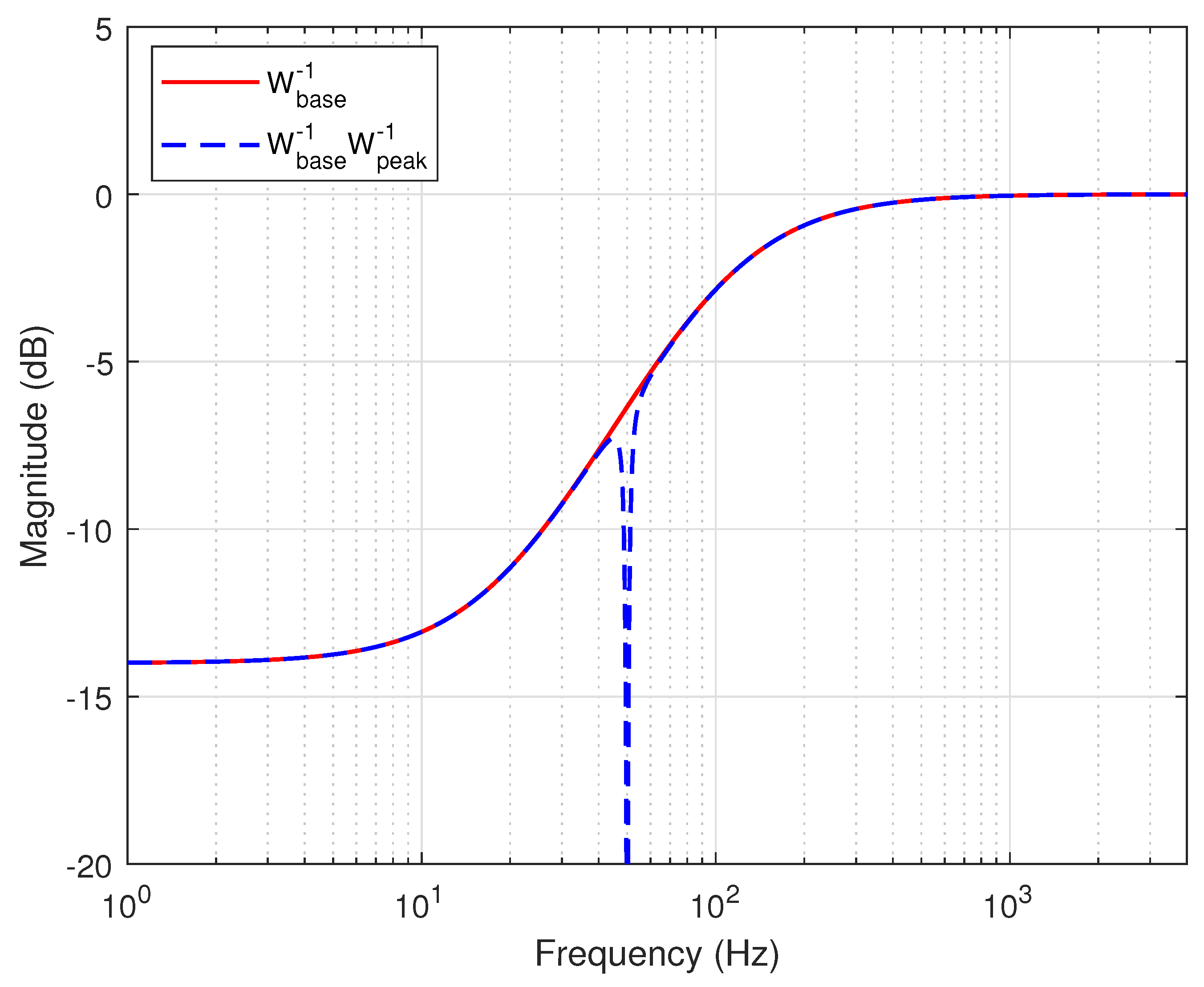
2.3. Optimal Disturbance Observer Design

To realize the proposed framework, all transfer functions should be described by state space representation. Here, P is the identified model and can be written by state space representation.

$$\begin{array}{c}\hfill P:\begin{array}{cc}\hfill \dot{x_P}\left(t\right)& =A_P{x}_P\left(t\right)+B_P{u}_P\left(t\right)\hfill \\ \hfill y_P\left(t\right)& =C_P{x}_P\left(t\right)\hfill \end{array}\end{array}$$

(7)

In addition, W and outer-loop controller C are described by state space representation, as in (8) and (9).

$$\begin{array}{c}\hfill W:\begin{array}{cc}\hfill \dot{x_W}\left(t\right)& =A_W{x}_W\left(t\right)+B_W{u}_W\left(t\right)\hfill \\ \hfill y_W\left(t\right)& =C_W{x}_W\left(t\right)+D_W{u}_W\left(t\right)\hfill \end{array}\end{array}$$

(8)

$$\begin{array}{c}\hfill C:\begin{array}{cc}\hfill \dot{x_C}\left(t\right)& =A_C{x}_C\left(t\right)+B_C{u}_C\left(t\right)\hfill \\ \hfill y_C\left(t\right)& =C_C{x}_C\left(t\right)+D_C{u}_C\left(t\right)\hfill \end{array}\end{array}$$

(9)

Considering (20), the system matrix of C is as follows.

$$\begin{array}{c}\hfill \begin{array}{cc}\hfill A_C& =A_n-B_{n}K-L{C}_n,\hfill \\ \hfill B_C& =-L,\hfill \\ \hfill C_C& =-K,\hfill \\ \hfill D_C& =0.\hfill \end{array}\end{array}$$

(10)

Using Equation (7), a state equation of P is calculated by

$$\begin{array}{c}\hfill \begin{array}{cc}\hfill {\dot{x}}_P\left(t\right)& =A_P{x}_P\left(t\right)+B_{P}w\left(t\right)\hfill \\ \hfill & +B_P(C_C{x}_C\left(t\right)+D_C{C}_P{x}_P\left(t\right))-B_P{u}_{DO}\left(t\right)\hfill \\ \hfill & =(A_P+B_P{D}_C{C}_P)x_P\left(t\right)+B_P{C}_C{x}_C\left(t\right)\hfill \\ \hfill & +B_{P}w\left(t\right)-B_P\left(t\right)u_{DO}\left(t\right).\hfill \end{array}\end{array}$$

(11)

A state equation of C is represented by

$$\begin{array}{c}\hfill \begin{array}{cc}\hfill {\dot{x}}_C\left(t\right)& =A_C{x}_C\left(t\right)+B_C{y}_{DO}\left(t\right)\hfill \\ \hfill & =A_C{x}_C\left(t\right)+B_C{C}_P{x}_P\left(t\right).\hfill \end{array}\end{array}$$

(12)

Moreover, a state equation of W can be calculated by

$$\begin{array}{c}\hfill \begin{array}{cc}\hfill {\dot{x}}_W\left(t\right)& =A_W{x}_W\left(t\right)+B_W(w\left(t\right)-u_{DO}\left(t\right))\hfill \\ \hfill & =A_W{x}_W\left(t\right)+B_{W}w\left(t\right)-B_W{u}_{DO}\left(t\right)).\hfill \end{array}\end{array}$$

(13)

z to be minimized is obtained by

$$\begin{array}{c}\hfill \begin{array}{cc}\hfill z\left(t\right)& =C_W{x}_W\left(t\right)+D_W(w\left(t\right)-u_{DO}\left(t\right))\hfill \\ \hfill & =C_W{x}_W\left(t\right)+D_{W}w\left(t\right)-D_W{u}_{DO}\left(t\right)).\hfill \end{array}\end{array}$$

(14)

and the input of the DO is captured as

$$\begin{array}{cc}\hfill y_{DO}\left(t\right)& =C_P{x}_P\left(t\right).\hfill \end{array}$$

(15)

Using Equations (11)–(15), the augmented systems are written as

$$\begin{array}{c}\hfill \begin{array}{cc}\hfill \dot{x}\left(t\right)& =Ax\left(t\right)+B_{1}w\left(t\right)+B_2{u}_{DO}\left(t\right)\hfill \\ \hfill z\left(t\right)& =C_{1}x\left(t\right)+D_{11}w\left(t\right)+D_{12}{u}_{DO}\left(t\right)\hfill \\ \hfill y_{DO}\left(t\right)& =C_{2}x\left(t\right)+D_{21}w\left(t\right)+D_{22}{u}_{DO}\left(t\right),\hfill \end{array}\end{array}$$

(16)

where $x\left(t\right)={\left[\begin{array}{ccc}{x}_p^T\left(t\right)& x_C^T\left(t\right)& x_W^T\left(t\right)\end{array}\right]}^T$, and

$$\begin{array}{c}\hfill \begin{array}{cc}\hfill A& =\left[\begin{array}{ccc}{A}_P+B_P{D}_C{C}_P& B_P{C}_C& 0\\ B_C{C}_P& A_C& 0\\ 0& 0& A_W\end{array}\right],\hfill \\ \hfill B_1& =\left[\begin{array}{c}{B}_p\\ 0\\ B_W\end{array}\right],B_2=\left[\begin{array}{c}-B_p\\ 0\\ -B_W\end{array}\right],\hfill \\ \hfill C_1& =\left[\begin{array}{ccc}0& 0& C_W\end{array}\right],D_{11}=D_W,D_{12}=-D_W,\hfill \\ \hfill C_2& =\left[\begin{array}{ccc}{C}_P& 0& 0\end{array}\right],D_{21}=0,D_{22}=0.\hfill \end{array}\end{array}$$

In addition, a state space representation of $C_{DO}$ is defined by

$$\begin{array}{c}\hfill C_{DO}:\begin{array}{cc}\hfill {\dot{x}}_{DO}\left(t\right)& =A_K{x}_{DO}\left(t\right)+B_K{y}_{DO}\left(t\right)\hfill \\ \hfill u_{DO}\left(t\right)& =C_K{x}_{DO}\left(t\right)+D_K{y}_{DO}\left(t\right)\hfill \end{array}\end{array}$$

(17)

Then, the closed loop systems, $T_{zw}$, can be obtained by

$$\begin{array}{cc}\hfill \left[\begin{array}{c}\dot{x}\left(t\right)\\ {\dot{x}}_{DO}\left(t\right)\end{array}\right]& =\left[\begin{array}{cc}A+B_2{D}_K{C}_2& B_2{C}_K\\ B_K{C}_2& A_K\end{array}\right]\left[\begin{array}{c}x\left(t\right)\\ x_{DO}\left(t\right)\end{array}\right]+\left[\begin{array}{c}{B}_1+B_2{D}_K{D}_{21}\\ B_K{D}_{21}\end{array}\right]w\left(t\right)\hfill \\ \hfill z\left(t\right)& =\left[\begin{array}{cc}{C}_1+D_{12}{D}_K{C}_2& D_{1}2C_K\end{array}\right]\left[\begin{array}{c}x\left(t\right)\\ x_{DO}\left(t\right)\end{array}\right]+\left[\begin{array}{c}{D}_{11}+D_{12}{D}_K{D}_{21}\end{array}\right]w\left(t\right).\hfill \end{array}$$

Theorem 1.

The following two statements are equivalent.

• ${\left|T_{zw}\right|}_{\infty }<\gamma$
• minimize γ subject to LMIs

  $$\begin{array}{c}\hfill \left[\begin{array}{cccc}AX+X{A}^T+B_{2}L+B_2^T{L}^T& A+B_{2}R{C}_2+Q^T& B_1+B_{2}R{D}_{21}& X{C}_1^T+L^T{D}_{12}\\ *& YA+A^{T}Y+F{C}_2+C_2^T{F}^T& Y{B}_1+F{D}_{21}& C_1^T+C_2^T{R}^T{D}_{12}^T\\ *& *& -I& D_{11}^T+D_{21}^T{R}^T{D}_{12}^T\\ *& *& *& -\gamma I\end{array}\right]<0,\\ \hfill \left[\begin{array}{cc}X& I\\ & Y\end{array}\right]>0\end{array}$$
  where $Q,F,L,R,X$, and Y are variables. $X>0$ means that X is positive definite and * denotes an ellipsis for terms induced by a symmetric matrix. Then, an optimal controller $C_{DO}^{*}$ is given by

  $$\begin{array}{c}\hfill \left[\begin{array}{cc}{A}_K& B_K\\ C_K& D_K\end{array}\right]=\left[\begin{array}{cc}{V}^{-1}& -V^{-1}Y{B}_2\\ 0& I\end{array}\right]\left[\begin{array}{cc}Q-YAX& F\\ L& R\end{array}\right]\left[\begin{array}{cc}{U}^{-1}& 0\\ -C_{2}X{U}^{-1}& I\end{array}\right],\end{array}$$
  where U and V are any nonsingular matrices satisfying $YX+VU=I$.

Proof of Theorem 1.

The result immediately follows from [37,39]. □

Theorem 2.

$C_{DO}^{*}$ stabilizes the closed loop systems.

Proof of Theorem 2.

Because $C_{DO}^{*}$ is a Lyapunov-stability-based $H_{\infty }$ dynamic output feedback controller, $C_{DO}^{*}$ always stabilizes the closed-loop systems [37,38,39]. □

3. Application Example

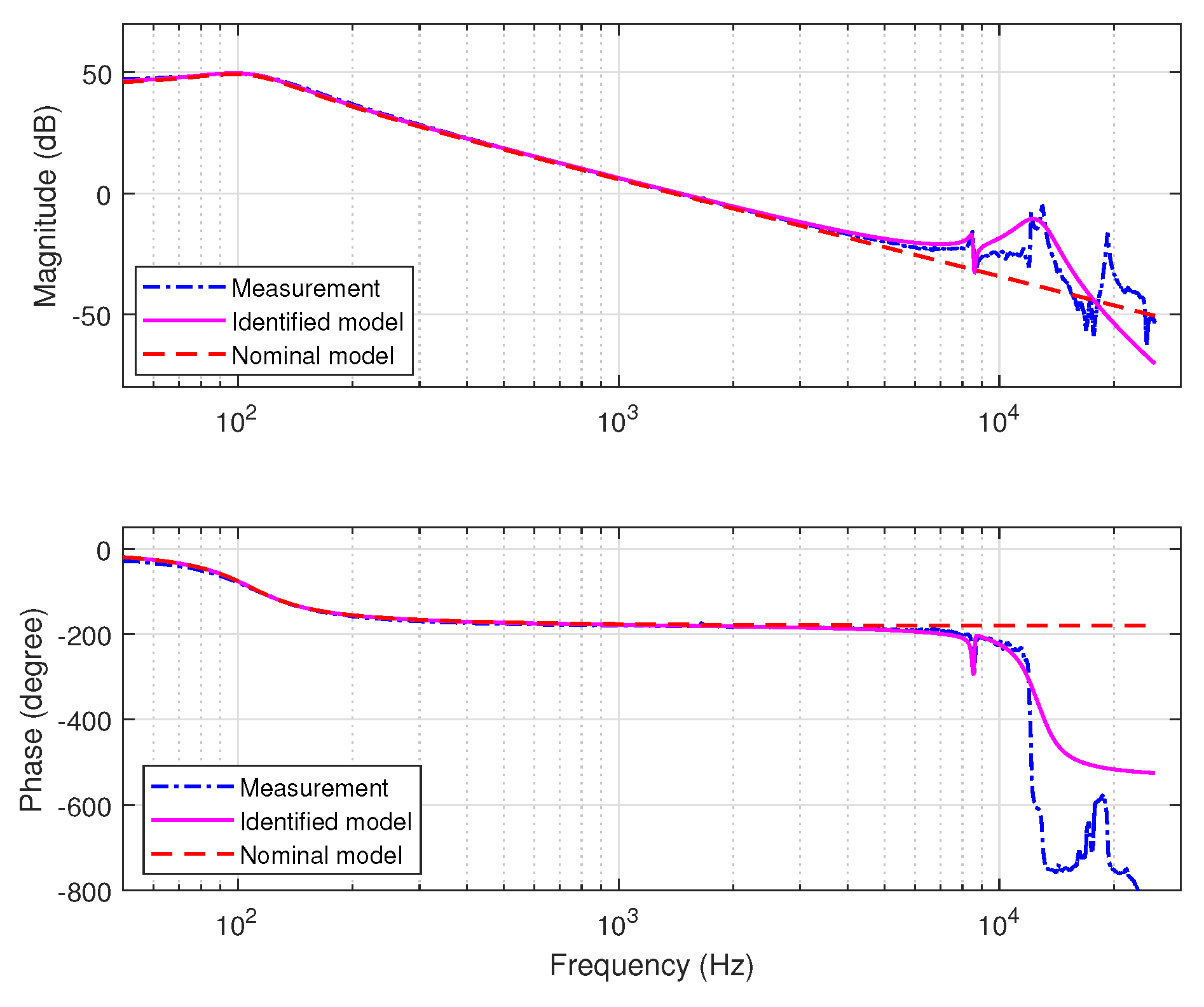
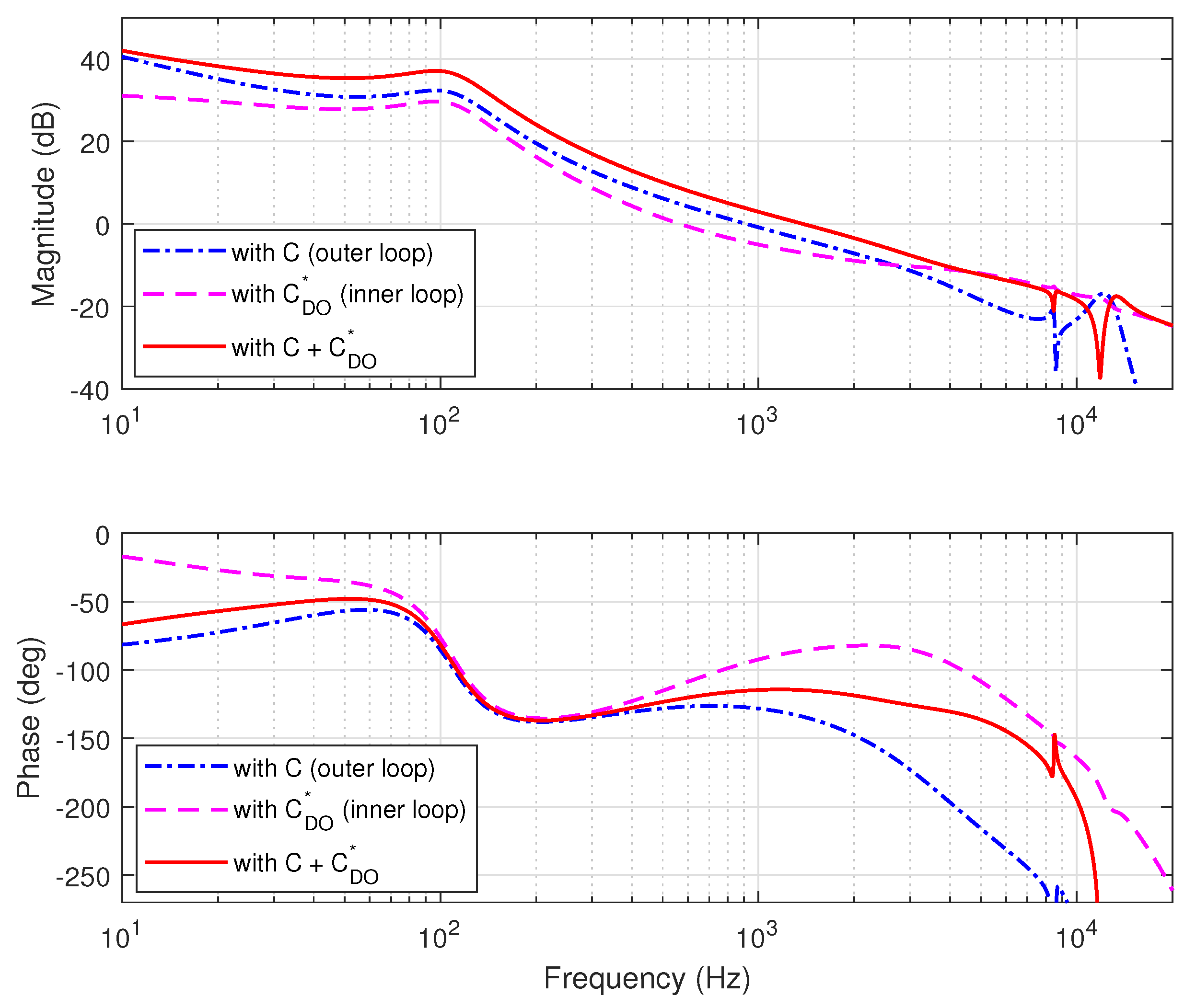
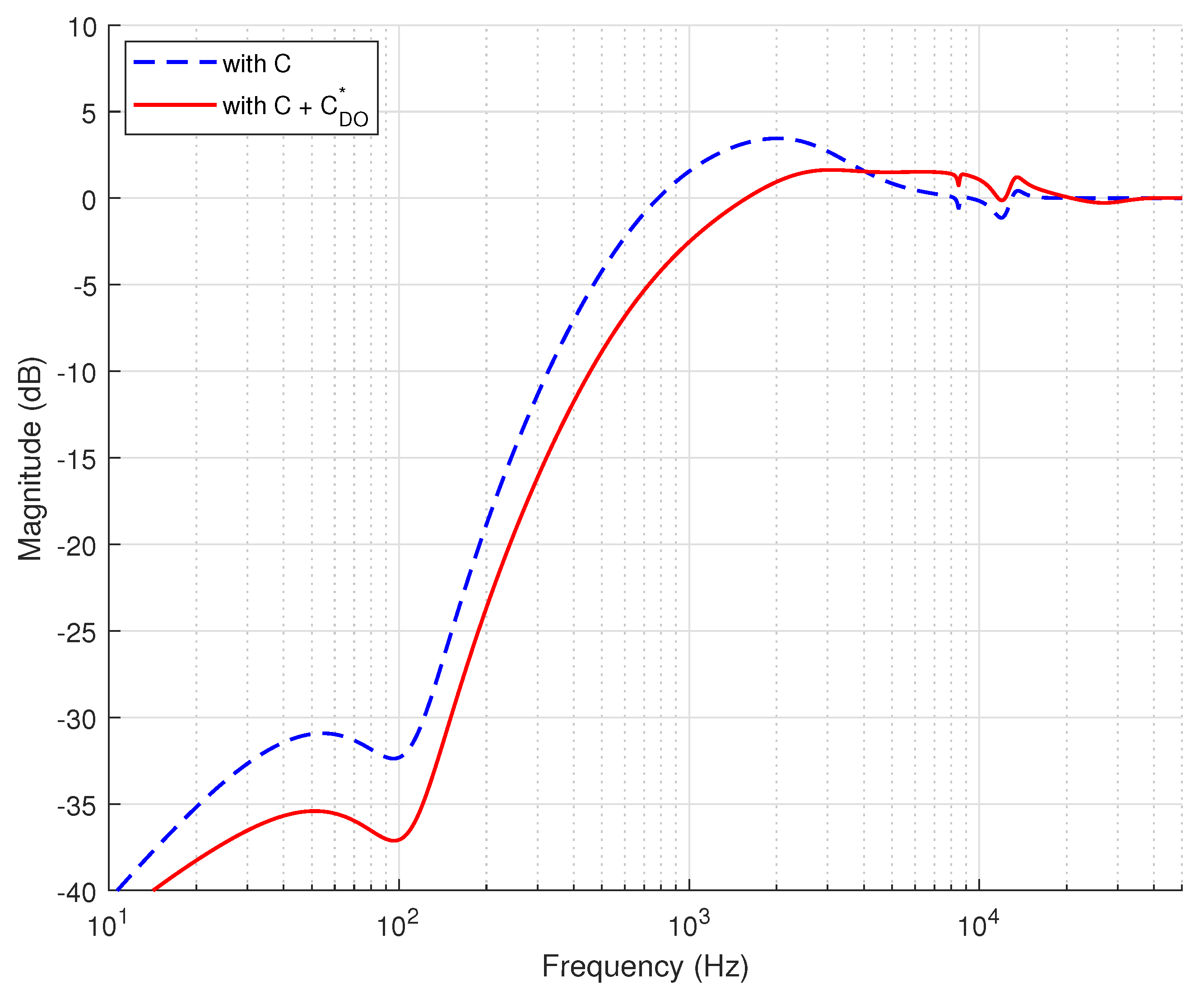
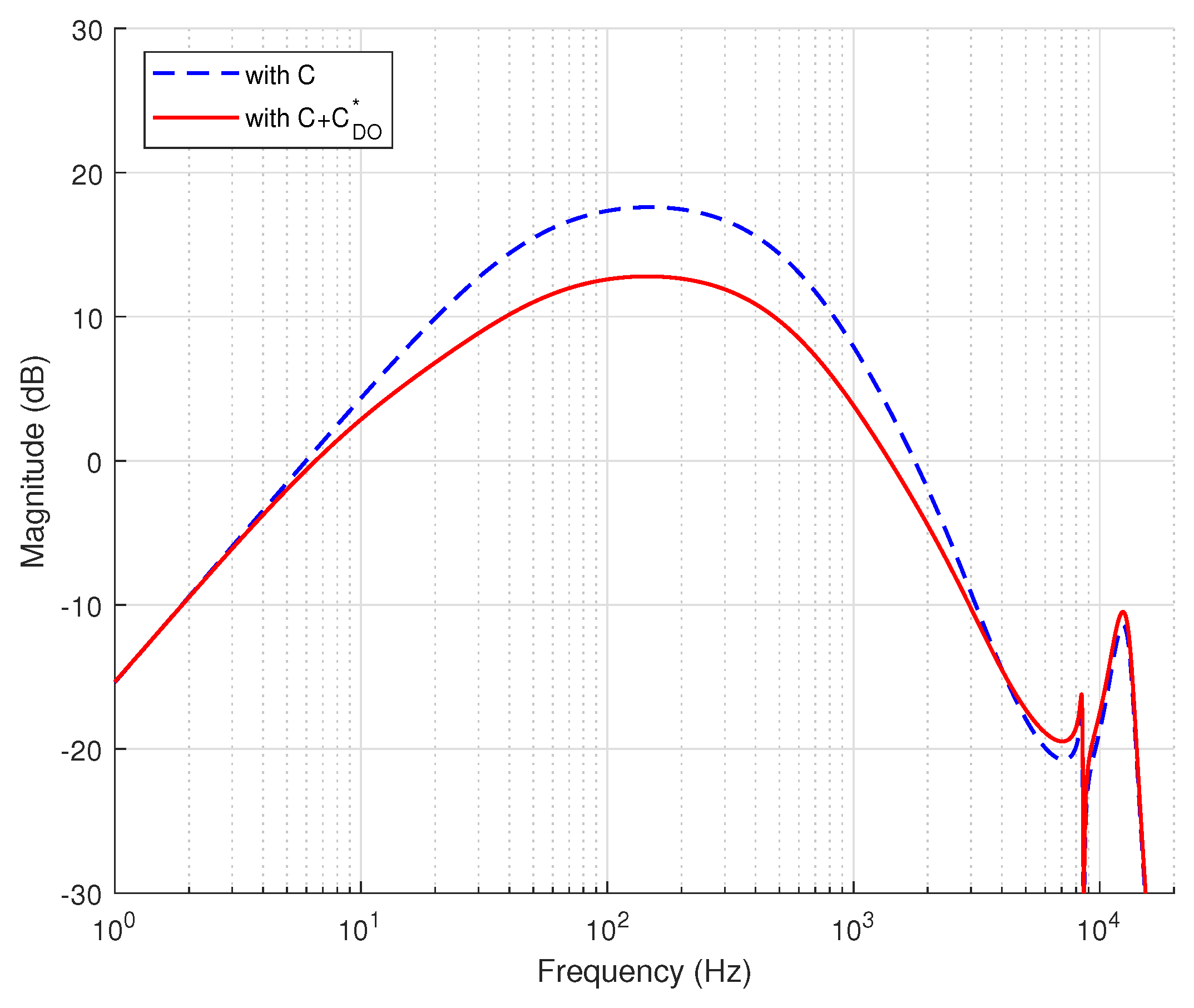
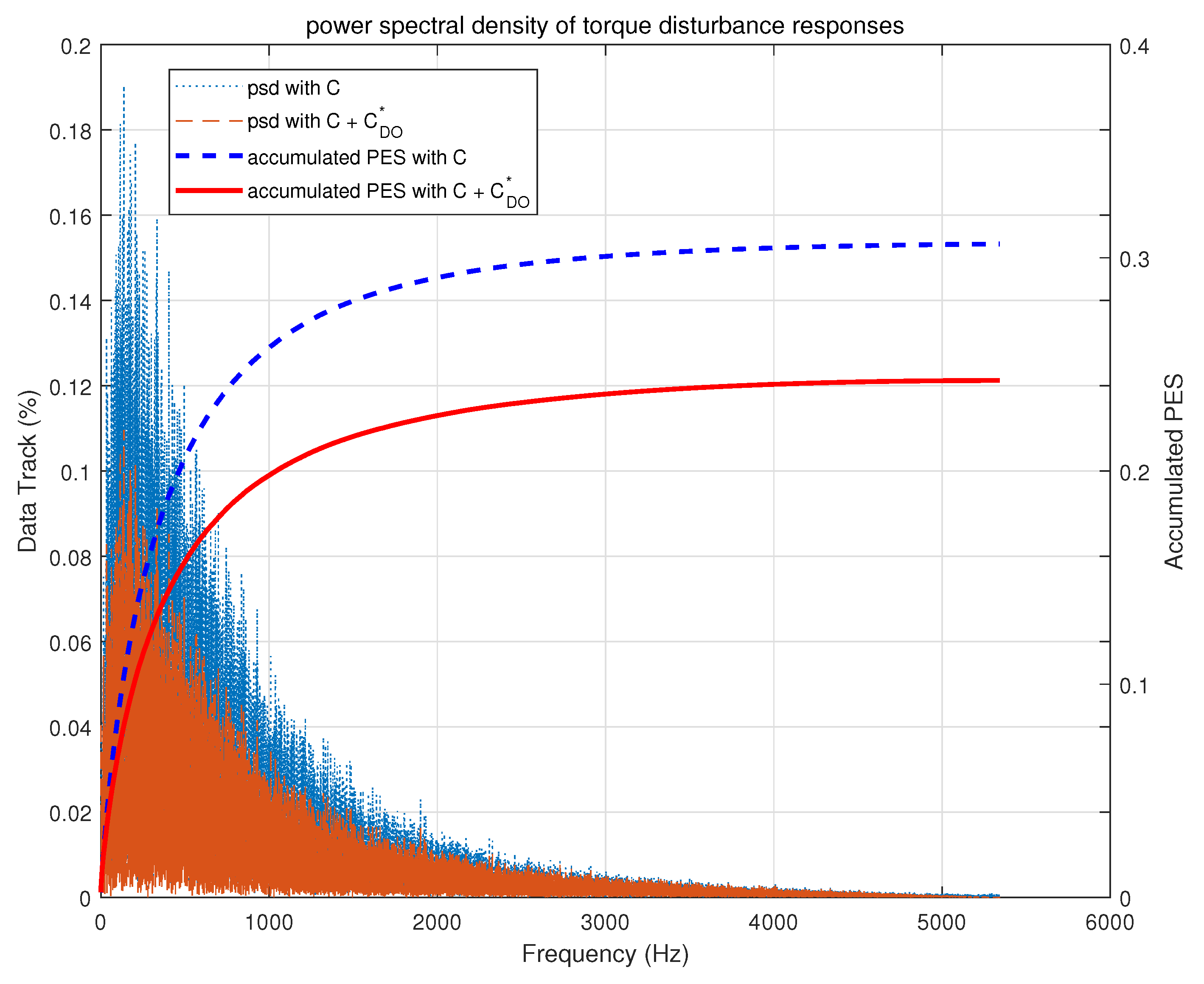
In this section, we applied the proposed method to two motion control systems—that is, hard disk drives (HDDs) and a pinhole camera model.

3.1. Case 1

Firstly, the proposed design method was applied to HDDs as a motion control system, as shown in Figure 4. The dynamics of a plant model were measured by a laser Doppler vibrometer (LDV) and a dynamic signal analyzer (DSA). The mathematical models are identified by

$$\begin{array}{c}\hfill \begin{array}{cc}\hfill P\left(s\right)& =\frac{K_t}{J_m}·\frac{1}{s^2+(B_d/J_m)s+K_s/J_m}·\frac{{\omega }_n^2}{s^2+2{\zeta }_n{\omega }_{n}s+{\omega }_n^2}·\prod _{i=1}^m\frac{s^2+2{\zeta }_{zi}{\omega }_{zi}s+{\omega }_{zi}^2}{s^2+2{\zeta }_{pi}{\omega }_{pi}s+{\omega }_{pi}^2}·\frac{{\omega }_{pi}^2}{{\omega }_{zi}^2}\hfill \end{array}\end{array}$$

(18)

where $K_t$ is the torque constant; $J_m$ is the inertia; $B_d$ is the damping coefficient, and $K_s$ is the damping coefficient; $K_s$ is the spring coefficient that determines low-frequency poles. Here, ${\omega }_n$ and ${\zeta }_n$ describe a baseline of high-frequency characteristics, and the remaining terms represent detailed high-frequency features over the baseline. For the high-frequency dynamics, $m=1$ is chosen. The values of the parameters are listed in

Table 1. HDDs parameters.

Parameter	Symbol	Value	Unit
torque constant	$K_t$	0.0046	$\mathrm{N}·\mathrm{m}/\mathrm{A}$
inertia	$J_m$	$0.95\times {10}^{-7}$	$\mathrm{kg}·{\mathrm{m}}^2$
damping coefficient	$B_d$	$3.8679\times {10}^{-5}$	$\mathrm{N}·\mathrm{s}/\mathrm{m}$
spring coefficient	$K_s$	0.0437	$\mathrm{N}/\mathrm{m}$
resonance frequency	${\omega }_n$	2$\pi$13,000	radian
damping ratio	${\zeta }_n$	0.1	-
resonance frequency	${\omega }_{zi}$	$2\pi 8600$	radian
damping ratio	${\zeta }_{zi}$	0.004	-
resonance frequency	${\omega }_{pi}$	$2\pi 8500$	radian
damping ratio	${\zeta }_{pi}$	0.01	-

.

Figure 4 shows the identified model and the nominal model.

For outer-loop design, a second-order nominal model is used. It is represented by the first two terms of the right side of Equation (18). Its state space model is expressed as

$$\begin{array}{c}\hfill P_n:\begin{array}{cc}\hfill {\dot{x}}_n\left(t\right)& =A_{n}x\left(t\right)+B_{n}u\left(t\right)\hfill \\ \hfill y_n\left(t\right)& =C_{n}x\left(t\right).\hfill \end{array}\end{array}$$

(19)

In this study, an estimator-based state feedback controller is designed to stabilize the plant as follows.

$$\begin{array}{c}\hfill C:\begin{array}{cc}\hfill \dot{\overline{x}}\left(t\right)& =A_n\overline{x}\left(t\right)+B_{n}u\left(t\right)+L(y_n\left(t\right)-C_n\overline{x}\left(t\right))\hfill \\ \hfill & =(A_n-B_{n}K-L{C}_n)\overline{x}\left(t\right)+L{y}_n\left(t\right)\hfill \\ \hfill u\left(t\right)& =-K\overline{x}\left(t\right),\hfill \end{array}\end{array}$$

(20)

where L and K are the estimator and state feedback control gains of C, respectively. To design the state feedback controller, a pole placement method is used [47]. In the outer-loop design, 914 Hz is chosen as the 0-dB crossover frequency, as stability margins, 12.4 dB and 52.6${}^{\circ }$ are used. For outer-loop design, estimator-based state feedback control was used. In the presence of disturbances, the proposed method was applied to remove the disturbances. Because only wide band disturbances were considered in this study, $W_{base}$ was used as a weight function. For weight function design, $M={10}^{0/20}$, $A={10}^{-14/20}$, ${\omega }_B^{*}=2\pi 100$ and $n=1$ were used. The designed weight function is represented by a red solid line in Figure 3. The designed open-loop transfer functions are shown in Figure 5. A dash-dotted line (blue) represents an open-loop transfer function of the inner loop, whereas a dashed line (magenta) represents an open-loop transfer function of the outer loop. A solid line (red) represents a combined open-loop transfer function of the inner and outer loops.

In the magnitude plot in Figure 5, the loop gain designed by $C_{DO}^{*}$ is added to the gain of the combined open-loop transfer function, and the additional gain results in an increasing 0-dB crossover frequency. Although it appears that $C_{DO}^{*}$ just adds gain, $C_{DO}^{*}$ also adds phase in the phase plot. This additional phase maintains or even increases the relative stability; in general, this advantage cannot be obtained by simple high-gain control.

Figure 6 shows Nyquist plots of the outer loop and the combined loop.

In the plot, $C_{DO}^{*}$ pushes the inner-loop transfer function to the right side, which indicates more stability margins, resulting in a lower peak in the sensitivity function. The maximum peak of the sensitivity function, S, is defined as

$$\begin{array}{c}\hfill \begin{array}{cc}\hfill M_S& =\underset{\omega }{max}\left|S\left(j\omega \right)\right|\hfill \\ \hfill & =\underset{\omega }{max}\left|{(1+L\left(j\omega \right))}^{-1}\right|\hfill \end{array}\end{array}$$

(21)

where L denotes an open-loop transfer function. Moreover, $1+L\left(j\omega \right)$ indicates the distance between $(-1,0)$ and $L\left(j\omega \right)$. The distance is represented by the radius of the circle tangent to $L\left(j\omega \right)$ and is located at $(-1,0)$. Furthermore, the radius is larger in more stable systems with more stability margins. In Figure 6, $r_2>r_1$, which implies that $C_{DO}^{*}$ offers more stability margins to the closed loop systems. Therefore, $C_{DO}^{*}$ decreases the peak of the sensitivity function. The compared sensitivity functions are shown in Figure 7.

In Figure 6, $r_1=0.67$ and $r_2=0.825$. Therefore, the corresponding sensitivity peaks are $20{log}_{10}(1/0.67)=3.48\mathrm{dB}$ and $20{log}_{10}(1/0.825)=1.67\mathrm{dB}$, respectively, as shown in Figure 7. As the sensitivity function is improved, the torque disturbance function is also is improved. The torque disturbance function is defined by a transfer function from plant input to plant output.

With $C_{DO}^{*}$, the peak of the torque disturbance function is reduced by 4.8 dB, as shown in Figure 8. The weight function W can control the performance of the disturbance rejection and frequency range of interest. The lower bound of $W^{-1}$ controls the performance of the disturbance rejection, and a cutoff frequency of $W^{-1}$ determines the frequency range of interest.

To measure the entire performance in all frequency ranges, random disturbances were applied to a zero-order hold equivalent discretized model with a sample frequency of 10.68 kHz. The measured power spectral density and accumulated position error signal (PES) are compared in Figure 9. With $C_{DO}^{*}$, the performance was improved by 20.9%.

For readability, the detailed results of the frequency responses are summarized in

Table 2. Summarized frequency characteristic.

	Without ${\mathit{C}}_{\mathbf{DO}}^{*}$	With ${\mathit{C}}_{\mathbf{DO}}^{*}$	Comment
$f_c$	914	1377	gain crossover frequency of open loop function (Hz)
GM	12.4	17.2	gain margin (dB)
PM	52.6	65.3	phase margin (${}^{\circ }$)
$f_s$	784	1580	bandwidth of sensitivity (Hz)
$M_S$	3.48	1.67	peak of sensitivity (dB)
$M_T$	17.6	12.8	peak of torque function (dB)
acc. PES	0.307	0.243	accumulated PES

.

3.2. Case 2

As for the second example, an optical image stabilization (OIS) system was used [41]. Because the identified model is a lightly damped system, a notch filter was firstly designed to suppress the oscillated responses of the plant. To design the outer loop controller C, an estimator-based state feedback controller was designed, as shown in Equation (20). In addition, a weight function was design, as shown in Figure 10, because hand shake disturbances exist in the frequency range below 100 Hz.

Using the weighting function, designed sensitivity functions were compared, as shown in Figure 11.

In the figure, the sensitivity peak is reduced, which implies that additional stabilities increase. In addition, the rejection performance to the plant output disturbances is also improved in the low frequency range. As the sensitivity function is improved, the torque disturbance function is improved, as shown in Figure 12.

In the figure, it is shown that the disturbance rejection performance is improved in the frequency range below 100 Hz. In particular, it shows a disturbance reduction effect of −15 dB at 1 Hz. This results from the weight function, as in Figure 10. As in the Section 3.1, in this Section 3.1, a random disturbance experiment was conducted. Figure 13 shows the compared power spectral densities. In OIS, error is defined by image pixel deviations because the parameter is crucial to image qualities.

With $C_{DO}^{*}$, an accumulated pixel deviation is improved by 36.3% in OIS.

4. Conclusions

An optimal DO was proposed in this paper. The proposed method does not require filters to resolve instability or compensators to solve causality problems. In addition, the designed DO always guarantees the stability of the closed-loop systems because predesigned outer-loop systems are considered as a model to be controlled and linear-matrix-inequality-based $H_{\infty }$ is applied. An application example verified that the proposed method is effective and improved the performance by 20.9% in HDDs and 36.6% in OIS.

References

1. Ohnishi, K. A New Servo Method in Mechatronics. Trans. Jpn. Soc. Electr. Eng. D 1987, 177, 83–86. [Google Scholar]
2. Yan, Y.; Yang, J.; Sun, Z.; Zhang, C.; Li, S.; Yu, H. Robust Speed Regulation for PMSM Servo System With Multiple Sources of Disturbances via an Augmented Disturbance Observer. IEEE/ASME Trans. Mechatron. 2018, 23, 769–780. [Google Scholar] [CrossRef]
3. Kim, W.; Chen, X.; Lee, Y.; Chung, C.C.; Tomizuka, M. Discrete-time Nonlinear Damping Backstepping Control with Observers for Rejection of Low and High Frequency Disturbances. Mech. Syst. Signal Process. 2018, 4, 436–448. [Google Scholar] [CrossRef]
4. Rafaq, M.S.; Nguyen, A.T.; Choi, H.H.; Jung, J.-W. A Robust High-Order Disturbance Observer Design for SDRE-Based Suboptimal Speed Controller of Interior PMSM Drives. IEEE Access 2019, 7, 165671–165683. [Google Scholar] [CrossRef]
5. Jo, N.H.; Jeon, C.; Shim, H. Noise Reduction Disturbance Observer for Disturbance Attenuation and Noise Suppression. IEEE Trans. Ind. Electron. 2017, 64, 1381–1391. [Google Scholar] [CrossRef]
6. Suh, S. Q filter design of disturbance observer for selective disturbance rejection. J. Inst. Control. Robot. Syst. 2019, 25, 105–110. [Google Scholar] [CrossRef]
7. Li, H.; Ning, X.; Han, B. Composite Decoupling Control of Gimbal Servo System in Double-Gimbaled Variable Speed CMG Via Disturbance Observer. IEEE/ASME Trans. Mechatron. 2017, 22, 312–320. [Google Scholar] [CrossRef]
8. Wang, F.; Wang, R.; Liu, E.; Zhang, W. Stabilization Control Mothed for Two-Axis Inertially Stabilized Platform Based on Active Disturbance Rejection Control With Noise Reduction Disturbance Observer. IEEE Access 2019, 7, 99521–99529. [Google Scholar] [CrossRef]
9. Ding, Z. Consensus Disturbance Rejection With Disturbance Observers. IEEE Trans. Ind. Electron. 2015, 62, 5829–5837. [Google Scholar] [CrossRef]
10. Ahmed, N.; Chen, M.; Shao, S. Disturbance Observer Based Tracking Control of Quadrotor With High-Order Disturbances. IEEE Access 2020, 8, 2169–3536. [Google Scholar] [CrossRef]
11. Ullah, I.; Pe, H.-L. Fixed Time Disturbance Observer Based Sliding Mode Control for a Miniature Unmanned Helicopter Hover Operations in Presence of External Disturbances. IEEE Access 2020, 8, 73173–73181. [Google Scholar] [CrossRef]
12. Chwa, D. Robust Nonlinear Disturbance Observer Based Adaptive Guidance Law Against Uncertainties in Missile Dynamics and Target Maneuver. IEEE Trans. Aerosp. Electron. Syst. 2018, 54, 1739–1749. [Google Scholar] [CrossRef]
13. Zhou, L.; Che, Z.; Yang, C. Disturbance Observer-Based Integral Sliding Mode Control for Singularly Perturbed Systems With Mismatched Disturbances. IEEE Access 2018, 6, 9854–9861. [Google Scholar] [CrossRef]
14. Elkayam, M.; Kolesnik, S.; Kuperman, A. Guidelines to Classical Frequency-Domain Disturbance Observer Redesign for Enhanced Rejection of Periodic Uncertainties and Disturbances. IEEE Trans. Power Electron. 2019, 34, 3986–3995. [Google Scholar] [CrossRef]
15. Ali, M.; Yaqoob, M.; Cao, L.; Loo, K.H. Disturbance-Observer-Based DC-Bus Voltage Control for Ripple Mitigation and Improved Dynamic Response in Two-Stage Single-Phase Inverter System. IEEE Trans. Ind. Electron. 2019, 66, 6836–6845. [Google Scholar] [CrossRef]
16. Li, M.; Shi, W.; Wei, J.; Fang, J.; Guo, K.; Zhang, Q. Parallel Velocity Control of an Electro-Hydraulic Actuator With Dual Disturbance Observers. IEEE Access 2019, 7, 56631–56641. [Google Scholar] [CrossRef]
17. Maeda, G.J.; Manchester, I.R.; Rye, D.C. Combined ILC and Disturbance Observer for the Rejection of Near-Repetitive Disturbances, With Application to Excavation. IEEE Trans. Control. Syst. Technol. 2015, 23, 1754–1769. [Google Scholar] [CrossRef]
18. Kim, W.; Shin, D.; Won, D.; Chung, C.C. Disturbance Observer Based Position Tracking Controller in the Presence of Biased Sinusoidal Disturbance for Electro-hydraulic Actuators. IEEE Trans. Control. Syst. Technol. 2013, 21, 2290–2298. [Google Scholar] [CrossRef]
19. Boukhnifer, M.; Ferreira, A. H Loop Shaping Bilateral Controller for a Two-Fingered Tele-Micromanipulation System. IEEE Trans. Control. Syst. Technol. 2007, 15, 891–905. [Google Scholar] [CrossRef]
20. Helfrich, B.E.; Lee, C.; Bristow, D.A.; Xiao, X.H.; Dong, J.; Alleyne, A.G.; Salapak, S.M.; Ferreir, P.M. Combined H-Feedback Control and Iterative Learning Control Design With Application to Nanopositioning Systems. IEEE Trans. Control. Syst. Technol. 2010, 18, 336–351. [Google Scholar] [CrossRef]
21. Sato, M.; Toda, M. Robust Motion Control of an Oscillatory-Base Manipulator in a Global Coordinate System. IEEE Trans. Ind. Electron. 2015, 62, 1163–1174. [Google Scholar] [CrossRef]
22. Bhaban, S.; Talukdar, S.; Li, M.; Hays, T.; Seiler, P.; Salapaka, M. Single Molecule Studies Enabled by Model-Based Controller Design. IEEE/ASME Trans. Mechatron. 2018, 23, 1532–1542. [Google Scholar] [CrossRef] [PubMed]
23. Zhang, X.; Koo, B.; Salapaka, S.M.; Dong, J.; Ferreira, P.M. Robust Control of a MEMS Probing Device. IEEE/ASME Trans. Mechatronics 2014, 19, 100–108. [Google Scholar] [CrossRef]
24. Yun, J.N.; Su, J. Robust Disturbance Observer for Two-Inertia System. IEEE Trans. Ind. Electron. 2013, 60, 2700–2710. [Google Scholar] [CrossRef]
25. Zhong, T.; Nagamune, R.; Yuen, A.; Tang, W. Online Estimation and Control for Feed Drive Systems With Unmeasurable Parameter Variations. IEEE Acess 2020, 8, 33966–33976. [Google Scholar] [CrossRef]
26. Yun, J.N.; Su, J.-B. Design of a Disturbance Observer for a Two-Link Manipulator With Flexible Joints. IEEE Trans. Control. Syst. Technol. 2014, 22, 809–815. [Google Scholar] [CrossRef]
27. Wang, L.; Su, J.; Xiang, G. Robust Motion Control System Design With Scheduled Disturbance Observer. IEEE Trans. Ind. Electron. 2016, 63, 6519–6529. [Google Scholar] [CrossRef]
28. Gassmann, V.; Knittel, D.; Pagill, P.R. Fixed-Order Tension Control in the Unwinding Section of a Web Handling System Using a Pendulum Dancer. IEEE Trans. Control. Syst. Technol. 2012, 20, 173–180. [Google Scholar] [CrossRef]
29. Huard, B.; Grossard, M.; Moreau, S.; Poinot, T. Sensorless Force/Position Control of a Single-Acting Actuator Applied to Compliant Object Interaction. IEEE Trans. Ind. Electron. 2015, 62, 3651–3661. [Google Scholar]
30. Chen, C.-S.; Chen, L.-Y. Robust Cross-Coupling Synchronous Control by Shaping Position Commands in Multiaxes System. IEEE Trans. Ind. Electron. 2012, 59, 4761–4773. [Google Scholar] [CrossRef]
31. Noshadi, A.; Shi, J.; Lee, W.S.; Shi, P.; Kalman, A. System Identification and Robust Control of Multi-Input Multi-Output Active Magnetic Bearing Systems. IEEE Trans. Control. Syst. Technol. 2016, 24, 1227–1239. [Google Scholar] [CrossRef]
32. Chen, X.; Yang, T.; Chen, X.; Zhou, K. A Generic Model-Based Advanced Control of Electric Power-Assisted Steering Systems. IEEE Trans. Control. Syst. Technol. 2008, 16, 1289–1300. [Google Scholar] [CrossRef]
33. Nie, J.; Conway, R.; Horowitz, R. Optimal H Control for Linear Periodically Time-Varying Systems in Hard Disk Drives. IEEE/ASME Trans. Mechatron. 2013, 18, 212–220. [Google Scholar] [CrossRef]
34. Lyu, X.; Zhou, J.; Gu, H.; Li, Z.; Shen, S.; Zhang, F. Disturbance Observer Based Hovering Control of Quadrotor Tail-Sitter VTOL UAVs Using H Synthesis. IEEE Robot. Autom. Lett. 2018, 3, 2910–2917. [Google Scholar] [CrossRef]
35. Lyu, X.; Zheng, M.; Zhang, F. H Based Disturbance Observer Design for Non-minimum Phase Systems with Application to UAV Attitude Control. In Proceedings of the Annual American Control Conference, Milwaukee, WI, USA, 27–29 June 2018; pp. 3683–3689. [Google Scholar]
36. Majumder, S.D. Flight optimisation of missile using linear matrix inequality (LMI) approach. J. Eng. 2020, 2020, 247–250. [Google Scholar] [CrossRef]
37. Boyd, S.; Ghaoui, L.E.; Feron, F.; Balakrishnan, V. Linear Matrix Inequalities in System and Control Theory; SIAM: Philadelphia, PA, USA, 1994. [Google Scholar]
38. Oliveira, C.D.; Geromel, J.C.; Bernussou, J. An LMI Optimization Approach to Multiobjective Controller Design for Discrete-Time Systems. In Proceedings of the 38th Conference on Decision and Control, Phoenix, AZ, USA, 7–10 December 1999; Volume 4, pp. 3611–3616. [Google Scholar]
39. Skelton, E.; Iwasaki, T.; Grigoriadis, K. A Unified Algebraic Approach to Linear Control Design; Taylor & Francis: Abingdon, UK, 1997. [Google Scholar]
40. Suh, S. Discrete-time controller design to attenuate effects of external disturbances. Microsyst. Technol. 2009, 15, 1645–1651. [Google Scholar] [CrossRef]
41. Suh, S. Stability driven optimal controller design for high quality images. Electronics 2018, 7, 437. [Google Scholar] [CrossRef] [Green Version]
42. Suh, S. ‘Unified H Control to Suppress Vertices of Plant Input and Output Sensitivity. IEEE Trans. Control. Syst. Technol. 2010, 18, 969–975. [Google Scholar] [CrossRef]
43. Suh, S. Estimation error based disturbance observer design for flexible loop shaping. Electronics 2018, 7, 358. [Google Scholar] [CrossRef] [Green Version]
44. Kim, W.; Suh, S. Suboptimal Disturbance Observer Design Using All Stabilizing Q Filter for Precise Tracking Control. Mathematics 2020, 8, 1434. [Google Scholar] [CrossRef]
45. Skogestad, S.; Postlethwaite, I. Multivariable Feedback Control: Analysis and Design; Wiley: New York, NY, USA, 1996. [Google Scholar]
46. Lam, H.Y.-F. Analog and Digital Filters; Prentice-Hall: Upper Saddle River, NJ, USA, 1979. [Google Scholar]
47. Franklin, G.F.; Powell, J.D.; Abbas, E.-N. Feedback Control of Dynamic Systems; Prentice-Hall: Upper Saddle River, NJ, USA, 2002. [Google Scholar]
Figure 1. Conventional DO.
Mathematics 08 01633 g001
Figure 2. Proposed framework for optimal DO design.
Mathematics 08 01633 g002
Figure 3. Weight functions to reject wide and narrow band disturbances.
Mathematics 08 01633 g003
Figure 4. Plant models: measured, identified, and nominal models.
Mathematics 08 01633 g004
Figure 5. Designed open loop transfer functions.
Mathematics 08 01633 g005
Figure 6. Nyquist plot and stability margins.
Mathematics 08 01633 g006
Figure 7. Designed sensitivity functions.
Mathematics 08 01633 g007
Figure 8. Designed torque transfer functions.
Mathematics 08 01633 g008
Figure 9. Compared power spectral densities.
Mathematics 08 01633 g009
Figure 10. Weight function for OIS.
Mathematics 08 01633 g010
Figure 11. Designed sensitivity functions.
Mathematics 08 01633 g011
Figure 12. Designed torque transfer functions.
Mathematics 08 01633 g012
Figure 13. Compared power spectral densities.
Mathematics 08 01633 g013