Numerical Solution of Stieltjes Differential Equations

Abstract

This work is devoted to the obtaining of a new numerical scheme based on quadrature formulae for the Lebesgue–Stieltjes integral for the approximation of Stieltjes ordinary differential equations. This novel method allows us to numerically approximate models based on Stieltjes ordinary differential equations for which no explicit solution is known. We prove several theoretical results related to the consistency, convergence, and stability of the numerical method. We also obtain the explicit solution of the Stieltjes linear ordinary differential equation and use it to validate the numerical method. Finally, we present some numerical results that we have obtained for a realistic population model based on a Stieltjes differential equation and a system of Stieltjes differential equations with several derivators.

1. Introduction

In this work, we present a numerical method in order to approximate the solution of a Stieltjes differential equation of the type:

$$\left\{\begin{array}{c}{x}_g^{\prime }\left(t\right)=f(t,x\left(t\right)),\mathrm{for}g\mathrm{almost}\mathrm{every}t\in [0,T),\hfill \\ x\left(0\right)=x_0,\hfill \end{array}\right.$$

(1)

where $x_g^{\prime }$ is the Stieltjes derivative with respect to a left-continuous non-decreasing function g. That is, given $x:[0,T]\to \mathbb{R}$, we define, for each $t\in [0,T]\backslash C_g$, $x_g^{\prime }\left(t\right)$ as the following limit in the case it exists:

$$x_g^{\prime }\left(t\right):=\left\{\begin{array}{cc}{\displaystyle \underset{s\to t}{lim}}\frac{x\left(s\right)-x\left(t\right)}{g\left(s\right)-g\left(t\right)},\hfill & \hfill \mathrm{if}t\notin D_g,\\ \frac{x\left(t^{+}\right)-x\left(t\right)}{g\left(t^{+}\right)-g\left(t\right)},\hfill & \hfill \mathrm{if}t\in D_g,\end{array}\right.$$

(2)

where $D_g$ denotes the set of discontinuities of g. In this particular case,

$$D_g=\{s\in \mathbb{R}:g\left(s^{+}\right)-g\left(s\right)>0\},$$

(3)

and

$$C_g=\{s\in \mathbb{R}:g\mathrm{is}\mathrm{constant}\mathrm{on}(s-\epsilon ,s+\epsilon )\mathrm{for}\mathrm{some}\epsilon \in {\mathbb{R}}^{+}\}.$$

(4)

Defining Equation (1) for “g almost every $t\in [0,T)$”, we are implicitly considering the Lebesgue–Stieltjes measure space $([0,T],{\mathcal{M}}_g,{\mu }_g)$, where ${\mathcal{M}}_g$ is the $\sigma$-algebra and ${\mu }_g$ the measure constructed in an analogous fashion to the classical Lebesgue measure, where the length of $[a,b)$ is given by ${\mu }_g\left([a,b)\right)=g\left(b\right)-g\left(a\right)$. The interested reader may refer to [1] for details concerning this measure space. The theoretical study of these kinds of derivatives and their applications appears, for instance, in [1,2,3,4,5], but can be traced back in the more general setting of fractional derivatives to [6]. More recent works in this direction include [7], where the authors studied $\Psi$-fractional derivatives.

As stated in [2] (Theorem 7.3), in the case $g:[0,T]\to [0,\infty )$ is increasing, left-continuous, and continuous at zero and $f:[0,T]\times \mathbb{R}\to \mathbb{R}$ satisfies:

Hypothesis 1.

$f(·,x)$ is g-measurable for every $x\in \mathbb{R}$;

Hypothesis 2.

$f(·,x_0)\in {\mathcal{L}}_g^1\left([0,T)\right)$, where ${\mathcal{L}}_g^1\left([0,T)\right)$ is the space of the equivalence classes of absolutely integrable functions with respect to the g Lebesgue–Stieltjes integral;

Hypothesis 3.

there exists $L\in {\mathcal{L}}_g^1([0,T),[0,\infty ))$ such that for g almost every $t\in [0,T)$ and every $x,y\in \mathbb{R}$, we have that:

$$|f(t,x)-f(t,y)|\le L\left(t\right)|x-y|;$$

(5)

Then, Problem (1) has a unique solution in the space ${\mathcal{BC}}_g\left([0,T]\right)$ of bounded g-continuous functions $u:[0,T]\to \mathbb{R}$, that is the solution u satisfies, for every $t_0\in [0,T]$,

$$\forall ϵ>0,\exists \delta >0:[t\in [0,T],|g\left(t\right)-g\left(t_0\right)|<\delta ]\Rightarrow |u\left(t\right)-u\left(t_0\right)|<ϵ.$$

(6)

${\mathcal{BC}}_g\left([0,T]\right)$ is a Banach space with the supremum norm—see [2] (Theorem 3.4). Furthermore, the solution of Problem (1) is the unique fixed point of the operator

$$\begin{array}{ccc}\hfill F:{\mathcal{BC}}_g\left([0,T]\right)& \to & {\mathcal{BC}}_g\left([0,T]\right),\hfill \\ \hfill x& \to & F\left(x\right),\hfill \end{array}$$

(7)

where given $t\in [0,T]$,

$$F\left(x\right)\left(t\right)=x_0+{\int }_{[0,t)}f(s,x\left(s\right))d{\mu }_g;$$

(8)

that is, the solution of Problem (1) is such that

$$x\left(t\right)=x_0+{\int }_{[0,t)}f(s,x\left(s\right))d{\mu }_g,\forall t\in [0,T].$$

(9)

Furthermore, from [2] (Lemma 7.2) and [1] (Theorem 5.4), the solution will belong to the space ${\mathcal{AC}}_g\left([0,T]\right)$ of g-absolutely continuous functions, that is, of those functions $u:[0,T]\to \mathbb{R}$ such that, for every $ϵ>0$, there exists $\delta >0$ satisfying that, if ${\left\{(a_n,b_n)\right\}}_{n\in \mathbb{N}}$ is a collection of pairwise-disjoint open intervals such that

$$\sum _{n=1}^N|g\left(b_n\right)-g\left(a_n\right)|<\delta ,$$

(10)

then,

$$\sum _{n=1}^N|f\left(b_n\right)-f\left(a_n\right)|<ϵ.$$

(11)

It is precisely Expression (9) that motivates the approximation based on the quadrature formulae for the Lebesgue–Stieltjes integral, which we introduce in Section 2. We will see that, in order to obtain error bounds, it will be necessary to impose additional conditions on the regularity of the function f and the solution of Problem (1).

In order to conveniently organize this work, in Section 2, we obtain some numerical quadrature formulae for approximating the Lebesgue–Stieltjes integral. In Section 3, we present a predictor-corrector method based on the quadrature formulae obtained in Section 2. In Section 4, we analyze mathematically the consistency, convergence, and stability of the numerical method derived in Section 3. In order to validate the numerical method, in Section 5, we obtain the explicit solution of the general linear equation of the Stieltjes type. Finally, in Section 6, we present some numerical results that we have obtained for the general linear equation and for realistic population models based on a Stieltjes differential equation.

2. Quadrature Formulae for the Lebesgue–Stieltjes Integral

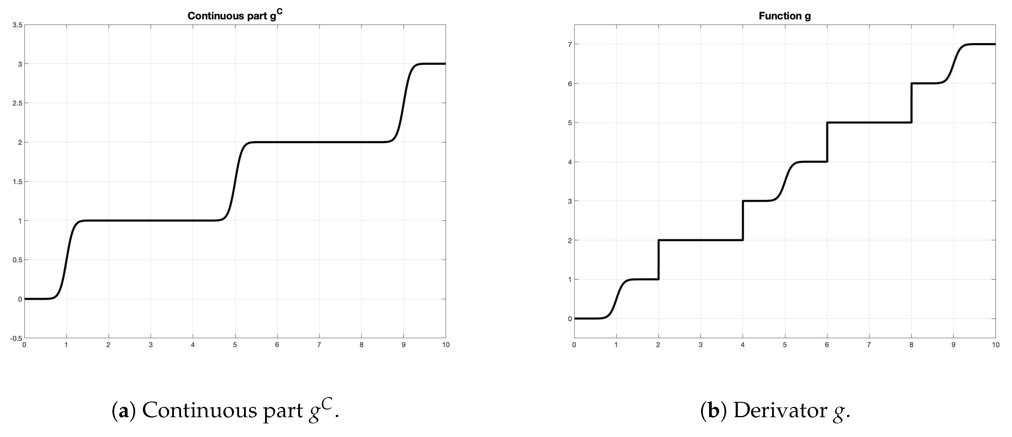
We now introduce some convenient notation. Given an increasing left-continuous function $g:[a,b]\to \mathbb{R}$, we define ${\Delta }^{+}g:[a,b)\to \mathbb{R}$ as ${\Delta }^{+}g\left(t\right)=g\left(t^{+}\right)-g\left(t\right)$. In the same way, we define ${\Delta }^{-}h\left(t\right)=h\left(t^{-}\right)-h\left(t\right)$ whenever the left limit of h exists at t. Clearly, g is continuous at $t_0\in [a,b)$ if and only if ${\Delta }^{+}g\left(t_0\right)=0$. It is important to point out the fact that the interval $[a,b]$ contains its right extremity, implying that the function g is bounded. We have that

$$0\le \sum _{t\in [a,b)}{\Delta }^{+}g\left(t\right)\le g\left(b\right)-g\left(a\right),$$

(12)

so g has a countable number of discontinuities, say those in $D_g={\left\{d_k\right\}}_{k\in \Lambda }$, where $\Lambda \subset \mathbb{N}$. If we define the bounded increasing function $g^B:[a,b)\to [0,+\infty )$ as

$$g^B\left(t\right)=\sum _{s\in [a,t)}{\Delta }^{+}g\left(s\right)={\Delta }^{+}g\left(a\right){\chi }_{(a,b]}\left(t\right)+\sum _{k\in \Lambda }{\Delta }^{+}g\left(d_k\right){\chi }_{(d_k,b]}\left(t\right),$$

(13)

it is clear that $g^C:[a,b)\to \mathbb{R}$, given by $g^C\left(t\right):=g\left(t\right)-g^B\left(t\right)$, is bounded, increasing, and continuous. We say $g^C$ is the continuous part of g and $g^B$ is the jump part of g.

As we mentioned in the previous section, the numerical method we propose to approximate the solution of the differential problem (1) in its integral form (9) will be based on the approximation of the Lebesgue–Stieltjes integral. We start this section by proving a result that will allow us to interpret the integral in (9) in terms of a Kurzweil–Stieltjes integral for which it will be possible to establish quadrature formulae. The Kurzweil–Stieltjes integral generalizes the Lebesgue–Stieltjes integral. On the one hand, it uses the gauge of the Henstock–Kurzweil integral in order to obtain an integral that is more powerful than that of Riemann (in fact, a function is Lebesgue integrable if and only if the function and its absolute value are Henstock–Kurzweil integrable); on the other hand, it uses the Stieltjes distribution function g in order to put a weight in the integral. The reader will find a comprehensive study of the Kurzweil–Stieltjes integral in [8].

Lemma 1.

Let $g:[a,b]\to [0,\infty )$ be an increasing left-continuous function and $f\in {\mathcal{L}}_g^1\left([a,b)\right)$. Then,

$${\int }_{[a,b)}fd{\mu }_g={\int }_a^{b}f\left(s\right)dg\left(s\right)={\int }_a^{b}f\left(s\right)d{g}^C\left(s\right)+\sum _{s\in [a,b)}f\left(s\right){\Delta }^{+}g\left(s\right),$$

(14)

where on the right-hand side, we consider a Kurzweil–Stieltjes integral. Furthermore, if ${\left\{d_k\right\}}_{k\in \Lambda }$ is the set of discontinuities of g in $(a,b)$, we have that

$${\int }_{[a,b)}fd{\mu }_g={\int }_a^{b}f\left(s\right)d{g}^C\left(s\right)+f\left(a\right){\Delta }^{+}g\left(a\right)+\sum _{k\in \Lambda }f\left(d_k\right){\Delta }^{+}g\left(d_k\right).$$

(15)

Proof. 

This lemma is an immediate consequence of [8] (Theorems 6.12.3 and 6.3.13). That is, since f is Lebesgue–Stieltjes integrable, by [8] (Theorem 6.12.3), it is Kurzweil–Stieltjes integrable as well, and furthermore,

$$\begin{array}{ccc}\hfill {\displaystyle {\int }_{[a,b)}fd{\mu }_g}& =& {\displaystyle {\int }_{\left\{a\right\}}fd{\mu }_g+{\int }_{(a,b)}fd{\mu }_g,}\hfill \\ \hfill {\displaystyle {\int }_{(a,b)}fd{\mu }_g}& =& {\displaystyle {\int }_a^{b}f\left(s\right)dg\left(s\right)-f\left(a\right){\Delta }^{+}g\left(a\right)-f\left(b\right){\Delta }^{-}g\left(b\right).}\hfill \end{array}$$

(16)

Now, due to the fact that g is left-continuous, ${\Delta }^{-}g\left(b\right)=0$, and since ${\mu }_g\left(\left\{a\right\}\right)={\Delta }^{+}g\left(a\right)$, we obtain:

$${\int }_{[a,b)}fd{\mu }_g={\int }_a^{b}f\left(s\right)dg\left(s\right).$$

(17)

Finally, by [8] (Theorem 6.3.13),

$$\begin{array}{cc}\hfill {\int }_a^{b}f\left(s\right)dg\left(s\right)=& {\int }_a^{b}f\left(s\right)d{g}^C\left(s\right)+f\left(a\right){\Delta }^{+}g\left(a\right)+f\left(b\right)\Delta g^{-}\left(b\right)+\sum _{k\in \Lambda }f\left(d_k\right)\Delta g\left(d_k\right).\hfill \end{array}$$

(18)

Since g is left-continuous, we have, in particular, that ${\Delta }^{-}g\left(b\right)={\Delta }^{-}g\left(d_k\right)=0$ for every $k\in \mathbb{N}$, and the desired result follows.  ☐

In Lemma 2, we will see that, under certain regularity hypotheses on f and g, we can obtain error estimates for the quadrature formula for a point and the trapeze formula.

Lemma 2.

Let us assume $f\in BV\left([a,b]\right)\cap {\mathcal{L}}_g^1\left([a,b)\right)$ and $g:[a,b]\to [0,\infty )$ is increasing and left-continuous. Furthermore, assume $g^C$ is p-H-Hölder on $[a,b]$, that is,

$$|g^C\left(x\right)-g^C{\left(y\right)|\le H|x-y|}^p,\forall x,y\in [a,b],$$

(19)

where $H>0$ and $p\in (0,1]$. Then,

$$\left|f\left(a\right)(g^C\left(b\right)-g^C\left(a\right))+\sum _{s\in [a,b)}f\left(s\right){\Delta }^{+}g\left(s\right)-{\int }_{[a,b)}fd{\mu }_g\right|\le H{(b-a)}^p{Var}_a^{b}f$$

(20)

and

$$\left|\frac{f\left(a\right)+f\left(b\right)}{2}(g^C\left(b\right)-g^C\left(a\right))+\sum _{s\in [a,b)}f\left(s\right){\Delta }^{+}g\left(s\right)-{\int }_{[a,b)}fd{\mu }_g\right|\le H{\left(\frac{b-a}{2}\right)}^p{Var}_a^{b}f.$$

(21)

Remark 1.

The previous quadrature formulae are most interesting in those cases where $D_g$ is finite, since in that case, the sums involved become finite.

Proof. 

Thanks to Lemma 1, it is enough to show that, if $g^C$ is p-H-Hölder on $[a,b]$ and $f\in BV\left(\right[a,b\left]\right)$, then

$${\displaystyle \left|f\left(a\right)(g^C\left(b\right)-g^C\left(a\right))-{\int }_a^{b}f\left(s\right)d{g}^C\left(s\right)\right|\le H{(b-a)}^p{Var}_a^{b}f,}$$

(22)

and

$${\displaystyle \left|\frac{f\left(a\right)+f\left(b\right)}{2}(g^C\left(b\right)-g^C\left(a\right))-{\int }_a^{b}f\left(s\right)d{g}^C\left(s\right)\right|\le H{\left(\frac{b-a}{2}\right)}^p{Var}_a^{b}f.}$$

(23)

Indeed, we can adapt the techniques in [9] for the Riemann–Stieltjes integral to the case of the Kurzweil–Stieltjes’. On the one hand, by [8] (Theorem 6.3.6), given that $h:[a,b]\to \mathbb{R}$ is continuous and $f\in BV\left(\right[a,b\left]\right)$, it holds that

$$\left|{\int }_a^{b}h\left(s\right)df\left(s\right)\right|\le \parallel h\parallel {Var}_a^{b}f.$$

(24)

On the other, thanks to [8] (Theorem 6.4.2) (integration by parts),

$$\begin{array}{cc}\hfill {\displaystyle {\int }_a^b\left[g^C\left(s\right)-\frac{g^C\left(a\right)+g^C\left(b\right)}{2}\right]df\left(s\right)=}& -{\int }_a^{b}f\left(s\right)d{g}^C\left(s\right)+{\left.\left[g^C\left(x\right)-\frac{g^C\left(a\right)+g^C\left(b\right)}{2}\right]f\left(x\right)\right|}_a^b\hfill \\ \hfill & +\sum _{a\le x\le b}\left(\Delta f^{-}\left(x\right){\Delta }^{-}{g}^C\left(x\right)-{\Delta }^{+}f\left(x\right){\Delta }^{+}{g}^C\left(x\right)\right),\hfill \end{array}$$

(25)

from which, given that $g^C$ is continuous,

$$\begin{array}{c}{\displaystyle {\int }_a^b\left[g^C\left(s\right)-\frac{g^C\left(a\right)+g^C\left(b\right)}{2}\right]df\left(s\right)=-{\int }_a^{b}f\left(s\right)d{g}^C\left(s\right)+\frac{f\left(a\right)+f\left(b\right)}{2}(g^C\left(b\right)-g^C\left(a\right)).}\end{array}$$

(26)

In particular,

$$\begin{array}{ccc}\hfill & \left|\frac{f\left(a\right)+f\left(b\right)}{2}(g^C\left(b\right)-g^C\left(a\right))-{\int }_a^{b}f\left(s\right)d{g}^C\left(s\right)\right|\le \hfill & \hfill \left|{\int }_a^b\left[g^C\left(s\right)-\frac{g^C\left(a\right)+g^C\left(b\right)}{2}\right]df\left(s\right)\right|.\end{array}$$

(27)

Let us define $h:t\in [a,b]\to h\left(t\right)$ as

$$h\left(t\right)=g^C\left(t\right)-\frac{g^C\left(a\right)+g^C\left(b\right)}{2}.$$

(28)

We have that

$$\begin{array}{ccc}\hfill {\displaystyle |h(t)|}& \le & {\displaystyle \left|\frac{g^C\left(t\right)-g^C\left(a\right)+g^C\left(t\right)-g^C\left(b\right)}{2}\right|}\hfill \\ \hfill & \le & {\displaystyle \frac{1}{2}|g^C\left(t\right)-g^C\left(a\right)|+\frac{1}{2}|g^C\left(b\right)-g^C\left(t\right)|}\hfill \\ \hfill & \le & {\displaystyle \frac{1}{2}H\left[{(t-a)}^p+{(b-t)}^p\right]\le H{\left(\frac{b-a}{2}\right)}^p,}\hfill \end{array}$$

(29)

for every $t\in [a,b]$. Then, thanks to the bound (24), we obtain the bound (23). In order to prove (22), we can proceed in an analogous fashion by integrating by parts

$$\begin{array}{c}{\displaystyle {\int }_a^b\left[g^C\left(s\right)-g^C\left(b\right)\right]df\left(s\right)=-{\int }_a^{b}f\left(s\right)d{g}^C\left(s\right)+{\left.\left[g^C\left(x\right)-g^C\left(b\right)\right]f\left(x\right)\right|}_a^b,}\end{array}$$

(30)

where we have already canceled out the terms concerning the sum. From the previous expression, we obtain

$$\left|f\left(a\right)(g^C\left(b\right)-g^C\left(a\right))-{\int }_a^{b}f\left(s\right)d{g}^C\left(s\right)\right|\le \left|{\int }_a^b[g^C\left(s\right)-g^c\left(b\right)]df\left(s\right)\right|\le H{(b-a)}^p{Var}_a^{b}f.$$

(31)

 ☐

As we will see later on, it will be of special interest to consider the case when $D_f\subset D_g$ and $f^C$ behaves in a similar way to $g^C$. In such a case, we can sharpen the previous quadrature formulae to obtain Lemma 5.

Definition 1.

Let $f:[a,b]\to \mathbb{R}$ and $g:[a,b]\to \mathbb{R}$ be left-continuous and increasing. We say f is g-Lipschitz continuous with Lipschitz constant H if $|f(t)-f(s)|\le H|g(t)-g(s)|$ for every $t,s\in [a,b]$.

Lemma 3.

Let $g:[a,b]\to \mathbb{R}$ be left-continuous and increasing $f:[a,b]\to \mathbb{R}$ g-Lipschitz continuous. Then, f is g-continuous, bounded, g-integrable, and of bounded variation.

Proof. 

It is clear that f is g-continuous. Since g is bounded and $|f(t)-f(s)|\le H|g(t)-g(s)|$ for every $t,s\in [a,b]$, f is bounded as well.

The g-integrability is a straightforward consequence of the definition of the Riemann–Stieltjes integral and the fact that f is g-continuous. Finally, ${Var}_a^{b}f\le H{Var}_a^{b}g=H(g\left(b\right)-g\left(a\right))$, so f is of bounded variation.  ☐

Corollary 1.

Let $g:[a,b]\to \mathbb{R}$ be left-continuous and increasing with $g^C$ being p-H-Hölder on $[a,b]$. Let $f:[a,b]\to \mathbb{R}$ be g-Lipschitz continuous with Lipschitz constant H. Then,

$$\begin{array}{c}{\displaystyle \left|f\left(a\right)(g^C\left(b\right)-g^C\left(a\right))-{\int }_a^{b}f\left(s\right)d{g}^C\left(s\right)\right|\le H^2{(b-a)}^p(g\left(b\right)-g\left(a\right)),}\end{array}$$

(32)

$$\begin{array}{c}{\displaystyle \left|\frac{f\left(a\right)+f\left(b\right)}{2}(g^C\left(b\right)-g^C\left(a\right))-{\int }_a^{b}f\left(s\right)d{g}^C\left(s\right)\right|\le H^2{\left(\frac{b-a}{2}\right)}^p(g\left(b\right)-g\left(a\right)).}\end{array}$$

(33)

The error estimates obtained in the previous formulae are not enough for our proposes, that is proving the convergence of the numerical approximation to the solution of Problem (1). In order to improve the previous estimations, we must add some extra requirements to the continuous part of functions g and f.

In the next lemma and corollary, we will prove that if f is a g-Lipschitz continuous function, some properties of $g^C$ and $g^B$ are transferred to $f^C$ and $f^B$, respectively. In particular, we will see that f is a g-Lipschitz continuous function and $g^C$ is Lipschitz continuous, then $f^C$ is also Lipschitz continuous. This property will be fundamental in order to improve the previous quadrature formula.

For the next lemma, we denote by $\mathfrak{C}\left(X\right)$ the set of connected components (in the usual topology) of $X\subset \mathbb{R}$.

Lemma 4.

Let $g:[a,b]\to \mathbb{R}$ be left-continuous in $(a,b)$ and increasing and $f:[a,b]\to \mathbb{R}$ be g-Lipschitz continuous with Lipschitz constant H. Then, $f^B$ is $g^B$-Lipschitz continuous with Lipschitz constant H. Furthermore, if f is increasing, then $f^C$ is $g^C$-Lipschitz continuous with Lipschitz constant H.

Proof. 

Let $t\in [a,b)$, $s\in (x,b)$. Then,

$${\displaystyle |f^B\left(s\right)-f^B\left(t\right)|\le |f\left(s\right)-f\left(t\right)|+|f^C\left(s\right)-f^C\left(t\right)|\le H(g\left(s\right)-g\left(t\right))+|f^C\left(s\right)-f^C\left(t\right)|.}$$

(34)

Thus, taking the limit when s tends to t from the right,

$$|{\Delta }^{+}f\left(t\right)|=|{\Delta }^{+}{f}^B\left(t\right)|\le H{\Delta }^{+}g\left(t\right)=H{\Delta }^{+}{g}^B\left(t\right).$$

(35)

Hence, for $t\in [a,b)$, $s\in (x,b)$,

$$\begin{array}{cc}\hfill |f^B\left(t\right)-f^B\left(s\right)|=& \left|\sum _{r\in [t,s)}{\Delta }^{+}f\left(r\right)\right|\le \sum _{r\in [t,s)}\left|{\Delta }^{+}f\left(r\right)\right|\le \sum _{r\in [t,s)}H{\Delta }^{+}g\left(r\right)=H(g^B\left(s\right)-g^B\left(t\right)).\hfill \end{array}$$

(36)

Therefore, $f^B$ is $g^B$-Lipschitz and g-Lipschitz with constant H.

We know that ${\sum }_{t\in [a,b)}{\Delta }^{+}g\left(t\right)<\infty$. This implies, on the one hand, that $D_g={\left\{t_n\right\}}_{n\in \Lambda }$ with $\Lambda \subset \mathbb{N}$ is countable and, on the other, that ${\Delta }^{+}g\left(t_n\right)\to 0$. Observe that g is continuous at b, and either g is continuous at a or $a=t_k$ for some $k\in \Lambda$. In this last case, we will assume, without loss of generality, that $a=t_1$.

Thus, consider, for $n\in \mathbb{N}$, the functions

$$\begin{array}{c}{f}_n\left(t\right):=f\left(t\right)-\sum _{\begin{array}{c}k\le n\\ k\in \Lambda \end{array}}{\Delta }^{+}f\left(t_k\right){\chi }_{(t_k,b]}\left(t\right)=f^C\left(t\right)+\sum _{\begin{array}{c}k>n\\ k\in \Lambda \end{array}}{\Delta }^{+}f\left(t_k\right){\chi }_{(t_k,b]}\left(t\right),\hfill \\ g_n\left(t\right):=g\left(t\right)-\sum _{\begin{array}{c}k\le n\\ k\in \Lambda \end{array}}{\Delta }^{+}g\left(t_k\right){\chi }_{(t_k,b]}\left(t\right)=g^C\left(t\right)-\sum _{\begin{array}{c}k>n\\ k\in \Lambda \end{array}}{\Delta }^{+}g\left(t_k\right){\chi }_{(t_k,b]}\left(t\right).\hfill \end{array}$$

(37)

Given $A\in \mathfrak{C}([a,b]\backslash {\left\{t_k\right\}}_{k=1}^n)$ (that is, an interval that is a connected component of $[a,b]\backslash {\left\{t_k\right\}}_{k=1}^n)$) and $t,s\in A$, $t<s$, since there are no jumps of ${\left\{t_k\right\}}_{k=1}^n$ in $[t,s]$, $f\left(s\right)-f\left(t\right)=f_n\left(s\right)-f_n\left(t\right)$ and $g\left(s\right)-g\left(t\right)=g_n\left(s\right)-g_n\left(t\right)$, so $|f_n\left(s\right)-f_n\left(t\right)|\le H|g_n\left(s\right)-g_n\left(t\right)|$. Define, for $t,s\in [a,b]$, $t\le s$,

$$\begin{array}{c}\hfill F_n(t,s):=H(g_n\left(s\right)-g_n\left(t\right))-(f_n\left(s\right)-f_n\left(t\right)).\end{array}$$

(38)

Since $F_n(t,s)\ge 0$ for every $t,s\in A$ and $f_n$ and $g_n$ are continuous at the points of $\partial A$, it also holds for $t,s\in \overline{A}$. Furthermore, $F_n(t,x)+F_n(x,s)=F_n(t,s)$. Hence, if $F_n(t,s)\ge 0$ for $t,s\in [\alpha ,\beta ]$ and $t,s\in [\beta ,\gamma ]$, then $F_n(t,s)\ge 0$ for $t,s\in [\alpha ,\gamma ]$. To see this, just observe that if $t\in [\alpha ,\beta ]$ and $s\in [\beta ,\gamma ]$, we consider $F_n(t,s)=F_n(t,\beta )+F_n(\beta ,s)\ge 0$.

Now, for any $t,s\in [a,b]$, $t<s$, either $[t,s]\cap {\left\{t_k\right\}}_{k=1}^n=\varnothing$; thus, $F_n(t,s)\ge 0$, or $[t,s]\cap {\left\{t_k\right\}}_{k=1}^n={\left\{t_k\right\}}_{k=p}^q$, and

$$F_n(t,s)=F_n(t,t_p)+F_n(t_p,t_{p+1})+\cdots +F_n(t_{q-1},t_q)+F_n(t_q,t)\ge 0.$$

(39)

We conclude that $F_n\ge 0$.

Observe now that $f_n$ converges uniformly to $f^C$ and $g_n$ converges uniformly to $g^C$, so $F_n$ converges uniformly to

$$\begin{array}{c}\hfill F(t,s):=H(g^C\left(s\right)-g^C\left(t\right))-(f^C\left(s\right)-f^C\left(t\right)).\end{array}$$

(40)

Since $F_n\ge 0$ for every $n\in \mathbb{N}$, $F\ge 0$, and thus, $f^C$ is $g^C$-Lipschitz continuous with Lipschitz constant H.  ☐

Corollary 2.

Let $g:[a,b]\to \mathbb{R}$ be left-continuous in $(a,b)$ and increasing and $f:[a,b]\to \mathbb{R}$ be g-Lipschitz continuous with Lipschitz constant H. Then, $f^C$ is $g^C$-Lipschitz continuous with Lipschitz constant H.

Proof. 

Since f is g-Lipschitz continuous, it is g-absolutely continuous and, by [1] (Theorem 5.4), there exists $f_g^{\prime }$${\mu }_g$-a.e. and $f\left(t\right)={\int }_{[a,t)}{f}_g^{\prime }\left(s\right)d{\mu }_g\left(s\right)$. Since f is g-Lipschitz continuous with Lipschitz constant H, for $s>t$,

$$\left|{\int }_{[t,s)}{f}_g^{\prime }\left(r\right)d{\mu }_g\left(r\right)\right|=|f\left(s\right)-f\left(t\right)|\le H(g\left(s\right)-g\left(t\right)).$$

(41)

Thus, by the definition of the Stieltjes g-derivative, $|f_g^{\prime }|\le H$${\mu }_g$-a.e.

Let $P={\left(f_g^{\prime }\right)}^{-1}\left({\mathbb{R}}^{+}\right)$ and $N=[a,b]\backslash P$. Define:

$$f_1\left(t\right)={\int }_{[a,t)\cap P}{f}_g^{\prime }\left(s\right)d{\mu }_g\left(s\right),f_2\left(t\right)=-{\int }_{[a,t)\cap N}{f}_g^{\prime }\left(s\right)d{\mu }_g\left(s\right).$$

(42)

Clearly, both $f_1$ and $f_2$ are g-Lipschitz continuous with Lipschitz constant H and increasing, so $f_1^C$ and $f_2^C$ are $g^C$-Lipschitz with Lipschitz constant H. Thus, $f^C=f_1^C-f_2^C$ is g-Lipschitz with Lipschitz constant H.  ☐

Corollary 3.

Let $g:[a,b]\to \mathbb{R}$ be continuous in $\{a,b\}$, left-continuous in $(a,b)$, and increasing and $f:[a,b]\to \mathbb{R}$ be g-Lipschitz continuous with Lipschitz constant H. If $g^C$ is Lipschitz continuous with Lipschitz constant H, then $f^C$ is Lipschitz continuous with Lipschitz constant $H^2$.

Proof. 

This is a direct consequence of the previous corollary since for all $s,t\in [a,b]$

$$|f^C\left(s\right)-f^C\left(t\right)|\le H|g^C\left(s\right)-g^C\left(t\right)|\le H^2|s-t|.$$

(43)

 ☐

In order to simplify the notation, from now on, we will assume, when necessary, that both the continuous part of f and the continuous part of g are Lipschitz continuous with the same Lipschitz constant H (if necessary, we redefine H to be $max\{H,H^2\}$).

Lemma 5.

Let $g:[a,b]\to \mathbb{R}$ be left-continuous and increasing and $f:[a,b]\to \mathbb{R}$ be g-Lipschitz continuous with Lipschitz constant H. We also assume that $f^C$ and $g^C$ are Lipschitz continuous with Lipschitz constant H. Then,

$$\begin{array}{cc}\hfill & \left|f^C\left(a\right)(g^C\left(b\right)-g^C\left(a\right))+\sum _{s\in [a,b)}\left[f\left(s\right){\Delta }^{+}g\left(s\right)+{\Delta }^{+}f\left(s\right)(g^C\left(b\right)-g^C\left(s\right))\right]-{\int }_{[a,b)}fd{\mu }_g\right|\hfill \\ \hfill =& \left|f^C\left(a\right)(g^C\left(b\right)-g^C\left(a\right))+f\left(a\right){\Delta }^{+}g\left(a\right)+{\Delta }^{+}f\left(a\right)(g^C\left(b\right)-g^C\left(a\right))\right.\hfill \\ & \left.+\sum _{k\in \Lambda }\left[f\left(d_k\right){\Delta }^{+}g\left(d_k\right)+{\Delta }^{+}f\left(d_k\right)(g^C\left(b\right)-g^C\left(d_k\right))\right]-{\int }_{[a,b)}fd{\mu }_g\right|\hfill \\ \hfill \le & H^2{(b-a)}^2,\hfill \end{array}$$

(44)

and

$$\begin{array}{cc}\hfill & \left|\frac{f^C\left(a\right)+f^C\left(b\right)}{2}(g^C\left(b\right)-g^C\left(a\right))\right.\hfill \\ & \left.+\sum _{s\in [a,b)}\left[f\left(s\right){\Delta }^{+}g\left(s\right)+{\Delta }^{+}f\left(s\right)(g^C\left(b\right)-g^C\left(s\right))\right]-{\int }_{[a,b)}fd{\mu }_g\right|\hfill \\ \hfill {\displaystyle =}& \left|\frac{f^C\left(a\right)+f^C\left(b\right)}{2}(g^C\left(b\right)-g^C\left(a\right))+f\left(a\right){\Delta }^{+}g\left(a\right)+{\Delta }^{+}f\left(a\right)(g^C\left(b\right)-g^C\left(a\right))\right.\hfill \\ & \left.+\sum _{k\in \Lambda }\left[f\left(d_k\right){\Delta }^{+}g\left(d_k\right)+{\Delta }^{+}f\left(d_k\right)(g^C\left(b\right)-g^C\left(d_k\right))\right]-{\int }_{[a,b)}fd{\mu }_g\right|\hfill \\ \hfill \le & \frac{H^2}{2}{(b-a)}^2,\hfill \end{array}$$

(45)

where ${\left\{d_k\right\}}_{k\in \Lambda }$ is the set of discontinuities of g in $(a,b)$.

Proof. 

First observe that, since f is g-continuous, $D_f\subset D_g$—see [2] (Proposition 3.2). Separating the jump part from the continuous part in both f and g, we have that:

$${\displaystyle {\int }_a^{b}f\left(s\right)dg\left(s\right)={\int }_a^b{f}^B\left(s\right)d{g}^B\left(s\right)+{\int }_a^b{f}^B\left(s\right)d{g}^C\left(s\right)+{\int }_a^b{f}^C\left(s\right)d{g}^B\left(s\right)+{\int }_a^b{f}^C\left(s\right)d{g}^C\left(s\right),}$$

(46)

where the three first integrals correspond to series and the fourth can be approximated using the previous quadrature formulae. Indeed, using analogous reasoning as that in [8] (Theorems 6.3.12 and 6.3.13):

$$\begin{array}{ccc}\hfill {\displaystyle {\int }_a^b{f}^B\left(s\right)d{g}^B\left(s\right)}& =& {\displaystyle f^B\left(a\right){\Delta }^{+}g\left(a\right)+\sum _{k\in \Lambda }{f}^B\left(d_k\right){\Delta }^{+}g\left(d_k\right)}\hfill \\ \hfill {\displaystyle {\int }_a^b{f}^B\left(s\right)d{g}^C\left(s\right)}& =& {\displaystyle {\Delta }^{+}f\left(a\right)(g^C\left(b\right)-g^C\left(a\right))+\sum _{k\in \Lambda }{\Delta }^{+}f\left(d_k\right)(g^C\left(b\right)-g^C\left(d_k\right)),}\hfill \\ \hfill {\displaystyle {\int }_a^b{f}^C\left(s\right)d{g}^B\left(s\right)}& =& {\displaystyle f^C\left(a\right){\Delta }^{+}g\left(a\right)+\sum _{k\in \Lambda }{f}^C\left(d_k\right){\Delta }^{+}g\left(d_k\right).}\hfill \end{array}$$

(47)

Taking that into account,

$$\begin{array}{ccc}\hfill {\displaystyle {\int }_a^{b}f\left(s\right)dg\left(s\right)}& =& {\displaystyle f\left(a\right){\Delta }^{+}g\left(a\right)+\sum _{k\in \Lambda }f\left(d_k\right){\Delta }^{+}g\left(d_k\right)+{\Delta }^{+}f\left(a\right)(g^C\left(b\right)-g^C\left(a\right))}\hfill \\ & & {\displaystyle +\sum _{k\in \Lambda }{\Delta }^{+}f\left(d_k\right)(g^C\left(b\right)-g^C\left(d_k\right))+{\int }_a^b{f}^C\left(s\right)d{g}^C\left(s\right).}\hfill \end{array}$$

(48)

Now, using the same argumentation as before,

$$\left|\frac{f^C\left(a\right)+f^C\left(b\right)}{2}(g^C\left(b\right)-g^C\left(a\right))-{\int }_a^b{f}^C\left(s\right)d{g}^C\left(s\right)\right|\le \frac{H^2}{2}{(b-a)}^2,$$

(49)

since ${Var}_a^b{f}^C\le H(b-a)$. The proof of identity (44) is analogous.  ☐

3. Description of the Numerical Method

In this section, we present a predictor-corrector method based on the previous quadrature formulae. We will assume $g:[0,T]\to \mathbb{R}$ is continuous at $t_0=0$ and that $D_g$ is finite. Let $x\in {\mathcal{BC}}_g\left([0,T]\right)$ be a solution of problem (1), and in what follows, let $f_{*}\left(x\right)\left(t\right):=f(t,x\left(t\right))$,

$$\begin{array}{cc}\hfill f_{*}^B\left(x\right)\left(t\right):=& \sum _{s\in [a,t)}{\Delta }^{+}{f}_{*}\left(x\right)\left(s\right),\hfill \\ \hfill f_{*}^C\left(x\right)\left(t\right):=& f_{*}\left(x\right)\left(t\right)-f_{*}^B\left(x\right)\left(t\right).\hfill \end{array}$$

(50)

Consider now a set ${\left\{t_k\right\}}_{k=0}^{N+1}\subset [0,T]$ satisfying:

Hypothesis 4.

$t_0=0$ and $t_{N+1}=T$; $t_{k+1}-t_k=h>0$, for every $k=0,\dots ,N$ and $D_g\subset {\left\{t_k\right\}}_{k=0}^{N+1}$. We denote this by $K_1=max\{{\Delta }^{+}g\left(d\right):d\in D_g\}$.

Hypothesis 5.

$f_{*}\left(x\right)$ is g-continuous, and in particular, $D_{f_{*}\left(x\right)}\subset D_g$ and $f_{*}^C\left(x\right)$ and $g^C$ are Lipschitz-continuous with the same Lipschitz constant H.

Hypothesis 6.

$f(·,c)\in {\mathcal{BC}}_g\left([0,T]\right)$, for every $c\in \mathbb{R}$.

Let us define $x_k:=x\left(t_k\right)$ and $x_k^{+}:=x\left(t_k^{+}\right)$, for $k=0,\dots ,N+1$. By the definition of the Stieltjes derivative,

$$x_k^{+}=x_k+{\Delta }^{+}g\left(t_k\right)f_{*}\left(x\right)\left(t_k\right),$$

(51)

and in the particular case $t_k\notin D_g$, ${\Delta }^{+}g\left(t_k\right)=0$, so we have that $x_k^{+}=x_k$. Then, for every $k=0,\dots ,N+1$,

$$x_{k+1}=x_k+{\int }_{[t_k,t_{k+1})}{f}_{*}\left(x\right)\left(s\right)dg\left(s\right),$$

(52)

where the integral is of the Kurzweil–Stieltjes type. Using (44) on each interval,

$$\begin{array}{ccc}\hfill {\displaystyle {\int }_{[t_k,t_{k+1})}{f}_{*}\left(x\right)\left(s\right)dg\left(s\right)}& \simeq & {\displaystyle f_{*}^C\left(x\right)\left(t_k\right)(g^C\left(t_{k+1}\right)-g^C\left(t_k\right))+f_{*}\left(x\right)\left(t_k\right){\Delta }^{+}g\left(t_k\right)}\hfill \\ & & {\displaystyle +{\Delta }^{+}{f}_{*}\left(x\right)\left(t_k\right)(g^C\left(t_{k+1}\right)-g^C\left(t_k\right)).}\hfill \end{array}$$

(53)

Thus, in the case that we use (45), we have:

$$\begin{array}{ccc}\hfill {\displaystyle {\int }_{[t_k,t_{k+1})}{f}_{*}\left(x\right)\left(s\right)dg\left(s\right)}& \simeq & {\displaystyle \frac{f_{*}^C\left(x\right)\left(t_k\right)+f_{*}^C\left(x\right)\left(t_{k+1}\right)}{2}(g^C\left(t_{k+1}\right)-g^C\left(t_k\right))}\hfill \\ & & {\displaystyle +f_{*}\left(x\right)\left(t_k\right){\Delta }^{+}g\left(t_k\right)+{\Delta }^{+}{f}_{*}\left(x\right)\left(t_k\right)(g^C\left(t_{k+1}\right)-g^C\left(t_k\right)).}\hfill \end{array}$$

(54)

Observe that the condition $D_g\subset {\left\{t_k\right\}}_{k=0}^{N+1}$ implies that, on each interval, the quadrature formulae lose the terms related to the interior jumps. Restricting to $[t_k,t_{k+1}]$, we have:

$$\begin{array}{ccc}\hfill {\displaystyle g^C\left(t\right)}& =& {\displaystyle g\left(t\right)-{\chi }_{(t_k,t_{k+1}]}{\Delta }^{+}g\left(t_k\right),}\hfill \\ \hfill {\displaystyle f_{*}^C\left(x\right)\left(t\right)}& =& {\displaystyle f_{*}\left(x\right)\left(t\right)-{\chi }_{(t_k,t_{k+1}]}{\Delta }^{+}{f}_{*}\left(x\right)\left(t_k\right).}\hfill \end{array}$$

(55)

Hence,

$$\begin{array}{ccc}\hfill {\displaystyle {\Delta }^{+}g\left(t_k\right)}& =& {\displaystyle g\left(t_k^{+}\right)-g\left(t_k\right),}\hfill \\ \hfill {\displaystyle g^C\left(t_k\right)}& =& {\displaystyle g\left(t_k\right),}\hfill \\ \hfill {\displaystyle g^C\left(t_{k+1}\right)}& =& {\displaystyle g\left(t_{k+1}\right)-g\left(t_k^{+}\right)+g\left(t_k\right),}\hfill \end{array}$$

(56)

and:

$$\begin{array}{ccc}\hfill {\displaystyle {\Delta }^{+}{f}_{*}\left(x\right)\left(t_k\right)}& =& {\displaystyle f(t_k^{+},x_k^{+})-f(t_k,x_k),}\hfill \\ \hfill {\displaystyle f_{*}^C\left(x\right)\left(t_k\right)}& =& {\displaystyle f(t_k,x_k),}\hfill \\ \hfill {\displaystyle f_{*}^C\left(x\right)\left(t_{k+1}\right)}& =& {\displaystyle f(t_{k+1},x_{k+1})-f(t_k^{+},x_k^{+})+f(t_k,x_k).}\hfill \end{array}$$

(57)

Taking into account the previous formulae, it is clear that, if we want to use (54) to approximate (52), the a-priori ignorance of the value $x_{k+1}$ forces us to estimate it. In order to do this, we just have to use (53), for which no further estimation is needed. That is, we will use (53) as the predictor and (54) as the corrector. Thus, the method will be as follows. Given $u_0=x_0$, we compute ${\left\{(u_{k-1}^{+},u_k^{*},u_k)\right\}}_{k=1}^{N+1}$ as:

$$\left\{\begin{array}{ccc}\hfill u_k^{+}& =& {\displaystyle u_k+f(t_k,u_k){\Delta }^{+}g\left(t_k\right),}\hfill \\ \hfill u_{k+1}^{*}& =& {\displaystyle u_k^{+}+f(t_k^{+},u_k^{+})(g\left(t_{k+1}\right)-g\left(t_k^{+}\right)),}\hfill \\ \hfill u_{k+1}& =& {\displaystyle u_k^{+}+\frac{1}{2}\left(f(t_k^{+},u_k^{+})+f(t_{k+1},u_{k+1}^{*})\right)(g\left(t_{k+1}\right)-g\left(t_k^{+}\right)).}\hfill \end{array}\right.$$

(58)

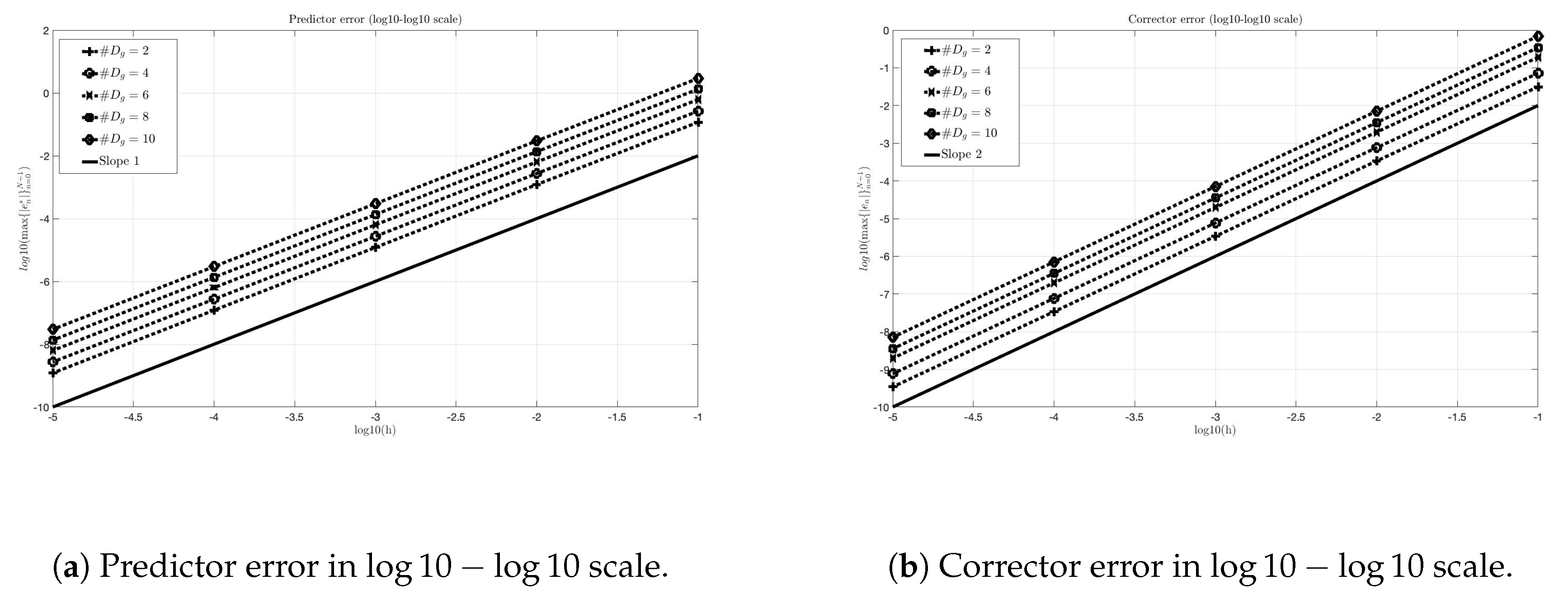
4. Error Analysis

In this section, we analyze the numerical method introduced in the previous one. As happens with those numerical methods based on quadrature formulae—cf. [10,11]—it will be crucial at this point to study the error of approximating the integral in this way.

As before, we will need certain regularity hypotheses on the derivator g, as well as on the function f when composed with the solution of the problem. Thus, we will assume Hypotheses 1–3 since they are necessary to guarantee the existence of Problem (1)—see page 2; Hypotheses 4–6, established in the previous sections in order to formulate the numerical method and the following additional hypotheses for proving the convergence of the method:

Hypothesis 7.

$f(t,·)\in {\mathcal{C}}^1\left(\mathbb{R}\right)$ for every $t\in \mathbb{R}$, and there exits $K_2\in \mathbb{R}$ such that

$$\left|\frac{\partial }{\partial x}f(t,x)\right|<K_2,$$

for every $(t,x)\in [0,T]\times \mathbb{R}$.

Hypothesis 8.

$f(t^{+},·)\in {\mathcal{C}}^1\left(\mathbb{R}\right)$ for every $t\in \mathbb{R}$, and there exits $K_3\in \mathbb{R}$ such that

$$\left|\frac{\partial }{\partial x}f(t^{+},x)\right|<K_3,$$

for every $(t,x)\in [0,T]\times \mathbb{R}$.

We must emphasize that the above hypotheses are not independent. For example, Hypothesis 6 implies Hypotheses 1 and 2, and Hypothesis 7 implies Hypothesis 3. Therefore, for our purposes, it is sufficient that Hypotheses 4–8 are fulfilled. We will now establish the basic notions related to the truncating error associated with the quadrature formula of the predictor-corrector method.

Definition 2 

(Local truncating error associated with the quadrature formula). Given a partition $P={\left\{t_k\right\}}_{k=0}^{N+1}$ satisfying (H4), we define:

• The local error associated with Formula (44) as:

  $${\sigma }_{k+1}^{*}:=x_{k+1}-x_k^{+}-f(t_k^{+},x_k^{+})(g\left(t_{k+1}\right)-g\left(t_k^{+}\right)),$$

  (59)

  with $k=0,\dots ,N$.
• The local error associated with Formula (45) as:

  $${\sigma }_{k+1}:=x_{k+1}-x_k^{+}-\frac{1}{2}\left(f(t_k^{+},x_k^{+})+f(t_{k+1},x_{k+1})\right)(g\left(t_{k+1}\right)-g\left(t_k^{+}\right)),$$

  (60)
  with $k=0,\dots ,N$.
• Letting

  $$x_{k+1}^{*}:=x_{k+1}-{\sigma }_{k+1}^{*}=x_k^{+}+f(t_k^{+},x_k^{+})(g\left(t_{k+1}\right)-g\left(t_k^{+}\right)),$$

  we define the local truncating error of the predictor-corrector method associated with (58), in terms of the exact solution, as:

  $$\begin{array}{c}{\displaystyle {\tau }_{k+1}:=x_{k+1}-x_k^{+}-\frac{1}{2}\left(f(t_k^{+},x_k^{+})+f(t_{k+1},x_{k+1}^{*})\right)(g\left(t_{k+1}\right)-g\left(t_k^{+}\right)),}\end{array}$$

  (61)

  with $k=0,\dots ,N$.

Remark 2.

It is usual to find in the literature local truncating errors defined relative to the discretization step h, that is ${\tilde{\sigma }}_{k+1}^{*}={\sigma }_{k+1}^{*}/h$, ${\tilde{\sigma }}_{k+1}={\sigma }_{k+1}/h$ and ${\tilde{\tau }}_{k+1}={\tau }_{k+1}/h$—cf. [10,11]. In those cases, for $k=0,\dots ,N$,

$$\begin{array}{cc}\hfill x_{k+1}=& x_k^{+}+f(t_k^{+},x_k^{+})(g\left(t_{k+1}\right)-g\left(t_k^{+}\right))+h{\tilde{\sigma }}_{k+1}^{*},\hfill \\ \hfill x_{k+1}=& x_k^{+}+\frac{1}{2}\left(f(t_k^{+},x_k^{+})+f(t_{k+1},x_{k+1})\right)(g\left(t_{k+1}\right)-g\left(t_k^{+}\right))+h{\tilde{\sigma }}_{k+1},\hfill \\ \hfill x_{k+1}=& x_k^{+}+\frac{1}{2}\left(f(t_k^{+},x_k^{+})+f(t_{k+1},x_{k+1}^{*})\right)(g\left(t_{k+1}\right)-g\left(t_k^{+}\right))+h{\tilde{\tau }}_{k+1}.\hfill \end{array}$$

(62)

We opted for the first set of errors in order to simplify the notation. In any case, the relation between both definitions is clear.

Now, we present some bounds of the errors.

Lemma 6.

For every $k=0,\dots ,N$, we have the following bounds:

• ${\displaystyle |{\sigma }_{k+1}^{*}|\le H^2{h}^2}$.
• ${\displaystyle |{\sigma }_{k+1}|\le \frac{1}{2}{H}^2{h}^2}$.
• ${\displaystyle |{\tau }_{k+1}|\le \frac{1}{2}{H}^2{h}^2+\frac{1}{2}{K}_2{H}^3{h}^3}$.

Proof. 

The two first assertions are a direct consequence of Lemma 5. In order to obtain the third one, we manipulate the definition of ${\tau }_{k+1}$, leaving:

$$\begin{array}{cc}\hfill {\displaystyle x_{k+1}=}& {\displaystyle x_k^{+}+\frac{1}{2}\left(f(t_k^{+},x_k^{+})+f(t_{k+1},x_{k+1}^{*})\right)(g(t_{k+1}-g\left(t_k^{+}\right))+{\tau }_{k+1}}\hfill \\ \hfill =& {\displaystyle x_k^{+}+\frac{1}{2}\left(f(t_k^{+},x_k^{+})+f(t_{k+1},x_{k+1})\right)(g\left(t_{k+1}\right)-g\left(t_k^{+}\right))}\hfill \\ \hfill & {\displaystyle +\frac{1}{2}\left(f(t_{k+1},x_{k+1}^{*})-f(t_{k+1},x_{k+1})\right)(g\left(t_{k+1}\right)-g\left(t_k^{+}\right))+{\tau }_{k+1},}\hfill \end{array}$$

(63)

from which we obtain, using the definition of ${\sigma }_{k+1}$,

$${\sigma }_{k+1}=\frac{1}{2}\left(f(t_{k+1},x_{k+1}^{*})-f(t_{k+1},x_{k+1})\right)(g\left(t_{k+1}\right)-g\left(t_k^{+}\right))+{\tau }_{k+1}.$$

(64)

By the mean value theorem of differential calculus, there exists $c_{k+1}$ in the open interval of extremities $x_{k+1}$, $x_{k+1}^{*}$ such that

$${\sigma }_{k+1}+\frac{1}{2}\frac{\partial f}{\partial x}(t_{k+1},c_{k+1}){\sigma }_{k+1}^{*}(g\left(t_{k+1}\right)-g\left(t_k^{+}\right))={\tau }_{k+1}.$$

(65)

Then, taking the absolute value,

$$|{\tau }_{k+1}|\le |{\sigma }_{k+1}|+\frac{1}{2}{K}_{2}H|{\sigma }_{k+1}^{*}|h.$$

(66)

Using the bounds obtained for $|{\sigma }_{k+1}|$ and $|{\sigma }_{k+1}^{*}|$,

$$|{\tau }_{k+1}|\le \frac{1}{2}{H}^2{h}^2+\frac{1}{2}{K}_2{H}^3{h}^3.$$

(67)

 ☐

Corollary 4

(Consistency of the numerical method). In the functional framework in which Lemma 6 is valid, the method is consistent.

Corollary 5.

Indeed, thanks to the bounds provided by Lemma 6, we obtain:

$$0\le \underset{h\to 0}{lim}\underset{0\le n\le N}{max}|{\tilde{\tau }}_{n+1}|\le \underset{h\to 0}{lim}\frac{1}{2}{H}^{2}h+\frac{1}{2}{K}_2{H}^3{h}^2=0,$$

(68)

from which we deduce the consistency of the method in the classical sense.

Remark 3.

In view of the bounds in Lemma 6, we must observe that the introduction of a predictor in the quadrature formula does not penalize its convergence order. This is due to the fact that ${\sigma }_{k+1}^{*}$ (which is the predictor term in the formula) appears multiplied by h in (66).

In our case, due to the regularity of the terms involved, we are not capable of improving the order of convergence of the two-point formula with respect to the one-point one. This is not usually the case, as in the literature, we can see examples—for instance [10,11]—where the two-point quadrature formula has a better convergence order—without the predictor penalizing the global order of the method—than the one-point one.

Definition 3

(Local error of the algorithm). We define the following errors associated with the numerical algorithm.

• $e_k^{+}:=u_k^{+}-x_k^{+}$, with $k=0,\dots ,N$, is the local error of the corrector regarding the limit from the right at $t_k$. It is clear that it does not make sense to consider this error for $k=N+1$.
• $e_k^{*}=u_k^{*}-x_k^{*}$, where $k=1,\dots ,N+1$, is the local error of the predictor at the point $t_k$.
• $e_k=u_k-x_k$, with $k=0,\dots ,N+1$ the local error of the predictor at the point $t_k$, and $e_0$ is the error associated with the initial condition.

In Lemma 7, we obtain bounds for the previous lemmata based on recurrence formulae, which, afterwards, we will analyze in order to obtain the bounds of the error at each of the points of the temporal discretization.

Lemma 7.

Under the hypotheses of Lemma 6, we derive the following formulae for $e_{k+1}^{*}$, $e_{k+1}$ and $e_k^{+}$, with $k=0,\dots ,N$,

• ${\displaystyle |e_k^{+}|\le \left[1+K_1{K}_2{\chi }_{D_g}\left(t_k\right)\right]|e_k|}$.
• ${\displaystyle |e_{k+1}^{*}|\le \left[1+K_{3}Hh+(1+K_{3}Hh)K_1{K}_2{\chi }_{D_g}\left(t_k\right)\right]|e_k|}$.
• ${\displaystyle |e_{k+1}|\le \left[1+G_1+G_2{\chi }_{D_g}\left(t_k\right)\right]|e_k|+{\tau }_{k+1}}$, where

  $$\begin{array}{cc}\hfill G_1=& {\displaystyle \frac{1}{2}{K}_{2}Hh+\frac{1}{2}{K}_{3}Hh+\frac{1}{2}{K}_3^2{H}^2{h}^2,}\hfill \\ \hfill G_2=& {\displaystyle K_1{K}_2+\frac{1}{2}{K}_1{K}_2{K}_{3}Hh+\frac{1}{2}{K}_1{K}_2^{2}Hh+\frac{1}{2}{K}_1{K}_2^2{K}_3{H}^2{h}^2.}\hfill \end{array}$$

  (69)

Proof. 

We compute each of the error bounds separately.

• Local error of the corrector regarding the limit from the right: We have that:

  $$\begin{array}{cc}\hfill e_k^{+}=& {\displaystyle u_k-x_k}\hfill \\ \hfill =& {\displaystyle u_k+f(t_k,u_k){\Delta }^{+}g\left(t_k\right)-x_k-f(t_k,x_k){\Delta }^{+}g\left(t_k\right)}\hfill \\ \hfill =& {\displaystyle e_k+\left(f(t_k,u_k)-f(t_k,x_k)\right){\Delta }^{+}g\left(t_k\right)}\hfill \\ \hfill =& {\displaystyle e_k+\frac{\partial f}{\partial x}(t_k,c_k)e_k{\Delta }^{+}g\left(t_k\right),}\hfill \end{array}$$

  (70)

  where $c_k$ belongs to the open interval of extremities $u_k$ and $x_k$. Taking the absolute value on both sides,

  $$\begin{array}{cc}\hfill {\displaystyle |e_k^{+}|\le |e_k|+K_1{K}_2|e_k|{\chi }_{D_k}\left(t_k\right),=}& {\displaystyle \left[1+K_1{K}_2{\chi }_{D_g}\left(t_k\right)\right]|e_k|.}\hfill \end{array}$$

  (71)
• Local error of the predictor at the point: We have:

  $$\begin{array}{cc}\hfill e_{k+1}^{*}=& {\displaystyle u_{k+1}^{*}-x_{k+1}}\hfill \\ \hfill =& {\displaystyle u_k^{+}+f(t_k^{+},u_k^{+})(g\left(t_{k+1}\right)-g\left(t_k^{+}\right))-x_k^{+}-f(t_k^{+},x_k^{+})(g\left(t_{k+1}\right)-g\left(t_k^{+}\right))}\hfill \\ \hfill =& {\displaystyle e_k^{+}+\left(f(t_k^{+},u_k^{+})-f(t_k^{+},x_k^{+})\right)(g\left(t_{k+1}\right)-g\left(t_k^{+}\right))}\hfill \\ \hfill =& {\displaystyle e_k^{+}+\frac{\partial f}{\partial x}(t_k^{+},c_k^{+})e_k^{+}(g\left(t_{k+1}\right)-g\left(t_k^{+}\right)),}\hfill \end{array}$$

  (72)

  where $c_k^{+}$ belongs to the open interval of extremities $u_k^{+}$ and $x_k^{+}$. Taking the absolute value on both sides,

  $$\begin{array}{cc}\hfill |e_{k+1}^{*}|\le & {\displaystyle \left[1+K_{3}Hh\right]|e_k^{+}|}\hfill \\ \hfill \le & {\displaystyle \left[1+K_{3}Hh\right]\left[1+K_1{K}_2{\chi }_{D_g}\left(t_k\right)\right]|e_k|}\hfill \\ \hfill =& {\displaystyle \left[1+K_{3}Hh+(1+K_{3}Hh)K_1{K}_2{\chi }_{D_g}\left(t_k\right)\right]|e_k|.}\hfill \end{array}$$

  (73)
• Local error of the predictor at the point: We have that

  $$\begin{array}{cc}\hfill |e_{k+1}|\le & {\displaystyle u_k^{+}+\frac{1}{2}(f(t_k^{+},u_k^{+})+f(t_{k+1},u_{k+1}^{*}))(g\left(t_{k+1}\right)-g\left(t_k^{+}\right))}\hfill \\ \hfill & {\displaystyle -x_k^{+}-\frac{1}{2}\left(f(t_k^{+},x_k^{+})+f(t_{k+1},x_{k+1}^{*})\right)(g(t_{k+1}-g\left(t_k^{+}\right))-{\tau }_{k+1}}\hfill \\ \hfill =& {\displaystyle |e_k^{+}|+\frac{1}{2}\left(f(t_k^{+},u_k^{+})-f(t_k^{+},x_k^{+})\right)(g\left(t_{k+1}\right)-g\left(t_k^{+}\right))}\hfill \\ \hfill & {\displaystyle +\frac{1}{2}\left(f(t_{k+1},u_{k+1}^{*})-f(t_{k+1},x_{k+1}^{*})\right)(g\left(t_{k+1}\right)-g\left(t_k^{+}\right))-{\tau }_{k+1}}\hfill \\ \hfill =& {\displaystyle |e_k^{+}|+\frac{1}{2}\frac{\partial f}{\partial x}(t_k^{+},c_k^{+})e_k^{+}(g\left(t_{k+1}\right)-g\left(t_k^{+}\right))}\hfill \\ \hfill & {\displaystyle +\frac{1}{2}\frac{\partial f}{\partial x}(t_{k+1},c_{k+1}^{*})e_{k+1}^{*}(g\left(t_{k+1}\right)-g\left(t_k^{+}\right))-{\tau }_{k+1},}\hfill \end{array}$$

  (74)

  where $c_k^{+}$ belongs to the open interval of extremities $u_k^{+}$, $x_k^{+}$ and $c_{k+1}^{*}$ belongs to the open interval of extremities $u_{k+1}^{*}$ and $x_{k+1}^{*}$. Taking the absolute value on both sides,

  $$\begin{array}{cc}\hfill |e_{k+1}|\le & {\displaystyle \left[1+\frac{1}{2}{K}_{3}Hh\right]|e_k^{+}|+\frac{1}{2}{K}_{2}Hh|e_{k+1}^{*}|+{\tau }_{k+1}}\hfill \\ \hfill \le & {\displaystyle \left[1+\frac{1}{2}{K}_{3}Hh\right]\left[1+K_1{K}_2{\chi }_{D_g}\left(t_k\right)\right]|e_k|}\hfill \\ \hfill & {\displaystyle +\frac{1}{2}{K}_{2}Hh\left[1+K_{3}Hh+(1+K_{3}Hh)K_1{K}_2{\chi }_{D_g}\left(t_k\right)\right]|e_k|+{\tau }_{k+1}}\hfill \\ \hfill =& {\displaystyle \left[1+G_1+G_2{\chi }_{D_g}\left(t_k\right)\right]|e_k|+{\tau }_{k+1},}\hfill \end{array}$$

  (75)

  where:

  $$\begin{array}{cc}\hfill G_1=& {\displaystyle \frac{1}{2}{K}_{2}Hh+\frac{1}{2}{K}_{3}Hh+\frac{1}{2}{K}_3^2{H}^2{h}^2,}\hfill \\ \hfill G_2=& {\displaystyle K_1{K}_2+\frac{1}{2}{K}_1{K}_2{K}_{3}Hh+\frac{1}{2}{K}_1{K}_2^{2}Hh+\frac{1}{2}{K}_1{K}_2^2{K}_3{H}^2{h}^2.}\hfill \end{array}$$

  (76)

 ☐

Remark 4.

Observe that previous error formulae can be simplified in the case $t_k\notin D_g$. In this situation, those errors concerning the limit from the right coincide with the ones of the corrector at the point, and we recover the classical error formulae.

From the formulae in Lemma 7, we can prove the following result concerning the error of the numerical method.

Lemma 8.

Under the hypotheses of Lemma 7, we have, for $n=0,\dots ,N$,

$$|e_{n+1}|\le {\left[1+G_2\right]}^{\#D_g}\left[|e_0|+\frac{\tau }{G_1}\right]exp\left[(n+1)G_1\right].$$

(77)

where $\tau =max\{|{\tau }_k|:k=1,\cdots ,N+1\}$.

Proof. 

Using the notation of Lemma 7, we have that

$$|e_{n+1}|\le \left[1+G_1+G_2{\chi }_{D_g}\left(t_n\right)\right]|e_n|+\tau .$$

(78)

Thus, applying the previous bound recursively,

$$\begin{array}{cc}\hfill {\displaystyle |e_{n+1}|\le }& {\displaystyle \prod _{k=0}^n\left[1+G_1+G_2{\chi }_{D_g}\left(t_k\right)\right]|e_0|+\sum _{k=1}^n\prod _{j=k}^n\left[1+G_1+G_2{\chi }_{D_g}\left(t_j\right)\right]\tau +\tau }\hfill \\ \hfill =& {\displaystyle \prod _{k=0}^n\left[1+G_2{\chi }_{D_g}\left(t_k\right)\right]\left[1+\frac{G_1}{1+G_2{\chi }_{D_g}\left(t_k\right)}\right]|e_0|}\hfill \\ \hfill & {\displaystyle +\sum _{k=1}^n\prod _{j=k}^n\left[1+G_2{\chi }_{D_g}\left(t_j\right)\right]\left[1+\frac{G_1}{1+G_2{\chi }_{D_g}\left(t_j\right)}\right]\tau +\tau .}\hfill \end{array}$$

(79)

Accounting for the number discontinuities of the derivator (which we denote by $\#D_g$), we obtain:

$${\displaystyle |e_{n+1}|\le {\left[1+G_2\right]}^{\#D_g}{\left[1+G_1\right]}^{n+1}+{\left[1+G_2\right]}^{\#D_g}\sum _{k=0}^n{\left[1+G_1\right]}^k\tau .}$$

(80)

Now, taking into account that, for a given number $G\ge 0$,

$$1+\sum _{k=0}^{n}G{(1+G)}^k={(1+G)}^{n+1}$$

(81)

and that $1+G\le exp\left(G\right)$, we have:

$$\begin{array}{cc}\hfill |e_{n+1}|\le & {\displaystyle {\left[1+G_2\right]}^{\#D_g}{\left[1+G_1\right]}^{n+1}+{\left[1+G_2\right]}^{\#D_g}\frac{\tau }{G_1}\sum _{k=0}^n{G}_1{(1+G_1)}^k}\hfill \\ \hfill \le & {\displaystyle {\left[1+G_2\right]}^{\#D_g}\left[|e_0|+\frac{\tau }{G_1}\right]{\left[1+G_1\right]}^{n+1}}\hfill \\ \hfill \le & {\displaystyle {\left[1+G_2\right]}^{\#D_g}\left[|e_0|+\frac{\tau }{G_1}\right]exp\left((n+1)G_1\right).}\hfill \end{array}$$

(82)

 ☐

Now, we will prove the main theorem of this section. In it, we will see that, in the framework of the previous results, we can guarantee the convergence of the method introduced in the previous section.

Theorem 1

(Convergence of the predictor-corrector method). Under the hypotheses of Lemma 5, if we assume $e_0=0$, we have, for a given $t_j\in [0,T]$, that

$$\begin{array}{ccc}{\displaystyle \underset{h\to 0}{lim}|u_j-x\left(t_j\right)|}\hfill & =& 0,\hfill \\ {\displaystyle \underset{h\to 0}{lim}|u_j^{*}-x^{*}\left(t_j\right)|}\hfill & =& 0,\hfill \\ {\displaystyle \underset{h\to 0}{lim}|u_j^{+}-x\left(t_j^{+}\right)|}\hfill & =& 0.\hfill \end{array}$$

(83)

Furthermore, we get the following error bounds:

$$\begin{array}{cc}\hfill {\displaystyle |u_j^{*}-x^{*}\left(t_j\right)|\le }& {\displaystyle \left[1+G_5{\chi }_{D_g}\left(t_j\right)\right]{\left[1+G_2\right]}^{\#D_g}\left[|e_0|+h\frac{\tau /h}{G_1}\right]exp\left[\frac{G_1}{h}{t}_j+G_4\right],}\hfill \\ \hfill {\displaystyle |u_j^{+}-x\left(t_j^{+}\right)|\le }& {\displaystyle \left[1+G_3{\chi }_{D_g}\left(t_j\right)\right]{\left[1+G_2\right]}^{\#D_g}\left[|e_0|+h\frac{\tau /h}{G_1}\right]exp\left[\frac{G_1}{h}{t}_j\right],}\hfill \\ \hfill {\displaystyle |u_j-x\left(t_j\right)|\le }& {\displaystyle {\left[1+G_2\right]}^{\#D_g}\left[|e_0|+h\frac{\tau /h}{G_1}\right]exp\left[\frac{G_1}{h}{t}_j\right],}\hfill \end{array}$$

(84)

for every $j=1,\dots ,N+1$, where

$$\begin{array}{ccc}\hfill G_3& =& {\displaystyle K_1{K}_2,}\hfill \\ \hfill G_4& =& {\displaystyle K_{3}Hh,}\hfill \\ \hfill G_5& =& {\displaystyle G_3(1+G_4).}\hfill \end{array}$$

(85)

Proof. 

We analyze each case separately.

• Errors associated with the corrector. From the previous lemma:

  $$\begin{array}{ccc}\hfill |e_{n+1}|& \le & {\displaystyle {\left[1+G_2\right]}^{\#D_g}\left[|e_0|+h\frac{\tau /h}{G_1}\right]exp\left[\frac{G_1}{h}(n+1)h\right],}\hfill \end{array}$$

  (86)

  where

  $$\begin{array}{cc}\hfill {\displaystyle \frac{\tau /h}{G_1}=}& \frac{H^2+K_2{H}^{3}h}{K_{2}H+K_{3}H+K_3^2{H}^{2}h}⟶\frac{H^2}{K_{2}H+K_{3}H}>0,\hfill \\ \hfill {\displaystyle \frac{G_1}{h}=}& \frac{1}{2}{K}_{2}H+\frac{1}{2}{K}_{3}H+\frac{1}{2}{K}_3^2{H}^{2}h⟶\frac{1}{2}{K}_{2}H+\frac{1}{2}{K}_{3}H>0,\hfill \end{array}$$

  (87)

  when $h\to 0$. Hence, given $t_j\in [0,T]$, we get

  $${\displaystyle |u_j-x\left(t_j\right)|\le {\left[1+G_2\right]}^{\#D_g}\left[|e_0|+h\frac{\tau /h}{G_1}\right]exp\left[\frac{G_1}{h}{t}_j\right].}$$

  (88)
  Then, given that $|e_0|=0$, we have the convergence of the corrector to the solution of the problem:

  $$\underset{h\to 0}{lim}{u}_j=x\left(t_j\right).$$

  (89)
• Errors associated with the predictor: Using the bounds in Lemmas 7 and 5, we have that, given $t_j\in [0,T]$,

  $$\begin{array}{ccc}\hfill |u_j^{*}-x^{*}\left(t_j\right)|& \le & {\displaystyle \left[1+K_{3}Hh+(1+K_{3}Hh)K_1{K}_2{\chi }_{D_g}\left(t_j\right)\right]|e_j|}\hfill \\ \hfill & \le & {\displaystyle \left[1+G_5{\chi }_{D_g}\left(t_j\right)\right]exp\left(G_4\right)|e_j|}\hfill \\ \hfill & \le & {\displaystyle \left[1+G_5{\chi }_{D_g}\left(t_j\right)\right]{\left[1+G_2\right]}^{\#D_g}\left[|e_0|+h\frac{\tau /h}{G_1}\right]exp\left[\frac{G_1}{h}{t}_j+G_4\right],}\hfill \end{array}$$

  (90)

  from which we obtain the convergence.
• Errors associated with the right limit: Using the bounds in Lemmas 7 and 5, we have that, given $t_j\in [0,T]$,

  $${\displaystyle |u_j^{+}-x\left(t_j^{+}\right)|\le \left[1+G_3{\chi }_{D_g}\left(t_j\right)\right]{\left[1+G_2\right]}^{\#D_g}\left[|e_0|+h\frac{\tau /h}{G_1}\right]exp\left[\frac{G_1}{h}{t}_j\right].}$$

  (91)
  We obtain the same kind of convergence as in the previous case. It is worth noting that, in the case $t_j\notin D_g$, the error associated with the right limit coincides with the error of the predictor.

 ☐

Remark 5.

Observe that the order of convergence of the method equals the order of τ minus one, that is of the order of $\tilde{\tau }$. In the case that we deal with functions with extra regularity, we may be able to improve the order of τ, which would better the order of convergence of the numerical method. Last, we would like to mention that the method we presented generalizes the classical order two Runge–Kutta. This assertion is motivated by the fact that the usual derivative is a particular instance of the Stieltjes derivative in the case $g\left(x\right)=x$.

Last, we analyze the stability of the method with the intention of evaluating its sensitivity towards the perturbations generated by the rounding errors produced while evaluating the different elements of Scheme (58). We omit the proof of the following result, as it is essentially a modification of that of Theorem 1.

Theorem 2

(Stability of the numerical method). Given ${\widehat{u}}_0$, we consider the following modification of the numerical scheme (58):

$$\left\{\begin{array}{ccc}\hfill {\displaystyle {\widehat{u}}_k^{+}}& =& {\displaystyle {\widehat{u}}_k+f(t_k,{\widehat{u}}_k){\Delta }^{+}g\left(t_k\right)+{\widehat{\rho }}_k^{+},}\hfill \\ \hfill {\displaystyle {\widehat{u}}_{k+1}^{*}}& =& {\displaystyle {\widehat{u}}_k^{+}+f(t_k,{\widehat{u}}_k^{+})(g\left(t_{k+1}\right)-g\left(t_k^{+}\right))+{\widehat{\rho }}_{k+1}^{*},}\hfill \\ \hfill {\displaystyle {\widehat{u}}_{k+1}}& =& {\displaystyle {\widehat{u}}_k^{+}+\frac{1}{2}\left(f(t_k,{\widehat{u}}_k^{+})+f(t_{k+1},{\widehat{u}}_{k+1}^{*})\right)(g\left(t_{k+1}\right)-g\left(t_k^{+}\right))+{\widehat{\rho }}_{k+1},}\hfill \end{array}\right.$$

(92)

where $k=0,\dots ,N$. Defining ${\widehat{e}}_k={\widehat{u}}_k-x\left(t_k\right)$, for $k=1,\dots ,N+1$, it holds that

$$|{\widehat{e}}_{k+1}|\le \left[1+G_1+G_2{\chi }_{D_g}\left(t_n\right)\right]|{\widehat{e}}_n|+|{\tau }_{k+1}|+|{\widehat{\rho }}_{k+1}|+G_1|{\widehat{\rho }}_k^{+}|+G_6|{\widehat{\rho }}_{k+1}^{*}|,$$

(93)

where

$$G_6=\frac{1}{2}{K}_{2}Hh.$$

(94)

Then, writing $\widehat{\rho }:=max\{|{\widehat{\rho }}_k|:k=1,\dots ,N+1\}$, ${\widehat{\rho }}^{*}=max\{|{\widehat{\rho }}_k^{*}|:k=1,\dots ,N+1\}$, and ${\widehat{\rho }}^{+}=max\{|{\widehat{\rho }}_k^{+}|:k=0,\dots ,N\}$, we have that, for every $t_j\in [0,T]$,

$${\displaystyle |{\widehat{u}}_j-x\left(t_j\right)|\le {\left[1+G_2\right]}^{\#D_g}\left[|e_0|+h\frac{\frac{\tau }{h}+\frac{\widehat{\rho }}{h}+G_1\frac{{\widehat{\rho }}^{+}}{h}+G_6\frac{{\widehat{\rho }}^{*}}{h}}{G_1}\right]exp\left[\frac{G_1}{h}{t}_j\right].}$$

(95)

5. The General Linear Equation

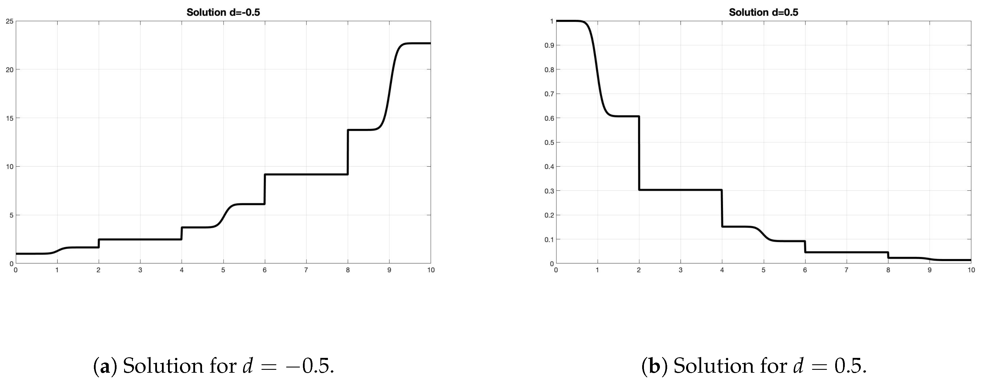
In order to validate the numerical approximation of the solution of Problem (1), we will consider the following general linear equation as a test problem:

$$\begin{array}{cc}\hfill x_g^{\prime }\left(t\right)+d\left(t\right)x\left(t\right)=& h\left(t\right),t\in [0,T),\hfill \\ \hfill x\left(0\right)=& x_0,\hfill \end{array}$$

(96)

where $x_0\in \mathbb{R}$, $h,d\in L_g^1\left([0,T)\right)$ and

$$\begin{array}{cc}\hfill & d\left(t\right){\Delta }^{+}g\left(t\right)\ne 1\forall t\in [a,b)\cap D_g,\hfill \end{array}$$

(97)

$$\begin{array}{cc}\hfill & \sum _{t\in [a,b)\cap D_g}\left|ln\left|1-d\left(t\right){\Delta }^{+}g\left(t\right)\right|\right|<\infty .\hfill \end{array}$$

(98)

Under (97) and (98), we know there is a unique solution of (96), which can be computed explicitly—see [2]—as the unique solution of the problem

$$\begin{array}{cc}\hfill x_g^{\prime }\left(t\right)+\tilde{d}\left(t\right)x\left(t^{+}\right)=& \tilde{h}\left(t\right),t\in [0,T),\hfill \\ \hfill x\left(0\right)=& x_0,\hfill \end{array}$$

(99)

where

$$\begin{array}{cc}\hfill \tilde{d}\left(t\right):=& \frac{d\left(t\right)}{1-d\left(t\right){\Delta }^{+}g\left(t\right)},\hfill \end{array}$$

(100)

$$\begin{array}{cc}\hfill \tilde{h}\left(t\right):=& \frac{h\left(t\right)}{1-d\left(t\right){\Delta }^{+}g\left(t\right)},\hfill \end{array}$$

(101)

are $L_g^1\left([0,T)\right)$ functions thanks to [2] (Proposition 6.8). Therefore, by [2] (Proposition 6.7), the solution of Problem (99) is given by

$$x\left(t\right):={\widehat{e}}_{\tilde{d}}^{-1}\left(t\right)\left(x_0+{\int }_{[0,t)}{\widehat{e}}_{\tilde{d}}\left(s\right)\tilde{h}\left(s\right)d{\mu }_g\left(s\right)\right),$$

(102)

where given an element $c\in L_g^1\left([0,T)\right)$,

$${\widehat{e}}_c\left(t\right):=\left\{\begin{array}{cc}exp\left({\int }_{[0,t)}\widehat{c}\left(s\right)d{\mu }_g\left(s\right)\right),\hfill & t\in [0,s_1],\hfill \\ {(-1)}^{k}exp\left({\int }_{[0,t)}\widehat{c}\left(s\right)d{\mu }_g\left(s\right)\right),\hfill & t\in [s_k,s_{k+1}],k=1,\cdots ,N,\hfill \end{array}\right.$$

(103)

$$\widehat{c}\left(t\right):=\left\{\begin{array}{ll}c\left(t\right)\hfill & t\in [0,T]\backslash D_g,\hfill \\ \frac{ln|1+c\left(t\right){\Delta }^{+}g\left(t\right)|}{{\Delta }^{+}g\left(t\right)},\hfill & t\in [0,T)\cap D_g,\hfill \end{array}\right.$$

(104)

$\{s_1,\cdots ,s_N\}=\{t\in [0,T)\cap D_g:1+c\left(t\right){\Delta }^{+}g\left(t\right)<0\}$ being the set of points such that $1+c\left(t\right){\Delta }^{+}g\left(t\right)<0$ and $s_{N+1}=T$. This set has finite cardinality—see [2] (Lemma 6.4). In our case, $c=\tilde{d}$; thus,

$$1+\tilde{d}\left(t\right){\Delta }^{+}g\left(t\right)=1+\frac{d\left(t\right){\Delta }^{+}g\left(t\right)}{1-d\left(t\right){\Delta }^{+}g\left(t\right)}=\frac{1}{1-d\left(t\right){\Delta }^{+}g\left(t\right)}<0$$

(105)

if and only if $1<d\left(t\right){\Delta }^{+}g\left(t\right)$. We will still denote by

$$\{s_1,\cdots ,s_N\}=\{t\in [0,T)\cap D_g:1-d\left(t\right){\Delta }^{+}g\left(t\right)<0\}$$

(106)

and $s_{N+1}=T$, so

$$\widehat{\tilde{d}}\left(t\right)=\left\{\begin{array}{cc}\tilde{d}\left(t\right)=d\left(t\right),\hfill & t\in [0,T]\backslash D_g,\hfill \\ \frac{ln|1+\tilde{d}\left(t\right){\Delta }^{+}g\left(t\right)|}{{\Delta }^{+}g\left(t\right)}=-\frac{ln|1-d\left(t\right){\Delta }^{+}g\left(t\right)|}{{\Delta }^{+}g\left(t\right)},\hfill & t\in [0,T)\cap D_g.\hfill \end{array}\right.$$

(107)

As we can see above, the general expression of the exponential ${\widehat{e}}_{\tilde{d}}\left(t\right)$, and therefore, of the solution of the general linear Equation (102), has a convoluted statement. This expression can be simplified if we consider the particular case where d is constant and $d{\Delta }^{+}g\left(t\right)<1$, $\forall t\in [a,b)\cap D_g$—the case that we will consider in the numerical experiments. In that case,

$$\begin{array}{cc}\hfill {\widehat{e}}_{\tilde{d}}\left(t\right)=& exp\left(dg\left(t\right)\right)exp\left[-\sum _{s\in [0,t)\cap Dg}\left(d{\Delta }^{+}g\left(s\right)+ln|1-d{\Delta }^{+}g\left(s\right)|\right)\right]\hfill \\ \hfill =& exp\left(dg\left(t\right)\right){\left[\prod _{s\in [0,t)\cap D_g}exp\left(d{\Delta }^{+}g\left(s\right)\right)|1-d{\Delta }^{+}g\left(s\right)|\right]}^{-1}.\hfill \end{array}$$

(108)

It is also remarkable that, in the case of $g\left(t\right)=t$, we recover the classical exponential. Furthermore, we have the following direct result for the problem with constant coefficients.

Theorem 3.

Let $g:[0,T]\to \mathbb{R}$ be increasing, left-continuous, and such that $g\left(0\right)=0$; $x_0\in \mathbb{R}$, $h\in \mathbb{R}$, and $d\in \mathbb{R}$ such that

$$\begin{array}{cc}\hfill & d{\Delta }^{+}g\left(t\right)<1\forall t\in [a,b)\cap D_g,\hfill \end{array}$$

(109)

$$\begin{array}{cc}\hfill & \sum _{t\in [a,b)\cap D_g}\left|ln(1-d{\Delta }^{+}g\left(t\right))\right|<\infty .\hfill \end{array}$$

(110)

Then, the solution of the problem

$$\begin{array}{cc}\hfill x_g^{\prime }\left(t\right)+dx\left(t\right)=& h,t\in [0,T),\hfill \\ \hfill x\left(0\right)=& x_0,\hfill \end{array}$$

(111)

is given by the following expression:

$$\begin{array}{cc}\hfill x\left(t\right)=& x_{0}exp(-dg\left(t\right))\left[\prod _{s\in [0,t)\cap D_g}exp\left(d{\Delta }^{+}g\left(s\right)\right)(1-d{\Delta }^{+}g\left(s\right))\right]\hfill \\ \hfill & +h{\int }_{[0,t)}exp\left(d(g\left(s\right)-g\left(t\right))\right)\left[\prod _{u\in (s,t)\cap D_g}exp\left(d{\Delta }^{+}g\left(u\right)\right)(1-d{\Delta }^{+}g\left(u\right))\right]d{\mu }_g\left(s\right).\hfill \end{array}$$

(112)

If we assume that the set of discontinuities of function g is finite and we consider a time discretization ${\left\{t_k\right\}}_{k=0}^{N+1}\subset [0,T]$ satisfying hypothesis (H4) with $d{\Delta }^{+}g\left(t\right)<1$, $\forall t\in [a,b)\cap D_g$, then the condition ${\sum }_{t\in [a,b)\cap D_g}\left|ln\left(1-d{\Delta }^{+}g\left(t\right)\right)\right|<\infty$ is trivially satisfied. Therefore, we have the following corollary for the homogenous case. The proof is straightforward.

Corollary 6.

Let $g:[0,T]\to \mathbb{R}$ be increasing and left-continuous, such that $g\left(0\right)=0$ with a set of discontinuity points that we can assume equal to the discretization points, that is $D_g=\{t_1,\cdots ,t_N\}\subset (0,T)$, where $t_k<t_{k+1}$ for $k=1,\cdots ,N-1$. Then, the solution of the problem

$$\begin{array}{cc}\hfill x_g^{\prime }\left(t\right)+dx\left(t\right)=& 0,t\in [0,T),\hfill \\ \hfill x\left(0\right)=& x_0,\hfill \end{array}$$

(113)

where $x_0,d\in \mathbb{R}$ and $d{\Delta }^{+}g\left(t\right)<1$, $\forall t\in [a,b)\cap D_g$, is given by:

$$x\left(t\right)=x_{0}exp(-dg\left(t\right))\left\{\begin{array}{cc}1,\hfill & t\in [0,t_1],\hfill \\ {\displaystyle \prod _{k=1}^n}(1-d{\Delta }^{+}g\left(t_k\right))exp\left(d{\Delta }^{+}g\left(t_k\right)\right),\hfill & t\in (t_n,t_{n+1}];n=1,\cdots ,N-1,\hfill \\ {\displaystyle \prod _{k=1}^N}(1-d{\Delta }^{+}g\left(t_k\right))exp\left(d{\Delta }^{+}g\left(t_k\right)\right),\hfill & t\in (t_N,T].\hfill \end{array}\right.$$

(114)

Finally, it is remarkable that, in the previous corollary, we can change the hypothesis $d{\Delta }^{+}g\left(t\right)<1$, $\forall t\in [a,b)\cap D_g$ by $d{\Delta }^{+}g\left(t\right)\ne 1$, $\forall t\in [a,b)\cap D_g$, and obtain a similar expression for the solution taking into account the general Formula (102). The last hypothesis is more general than the previous one, but in order to present the results in a clear way, we will assume that the first hypothesis is fulfilled.

6. Numerical Simulations

In this section we will present some numerical results that we reached using the scheme (58) for approximating the solution of the homogeneous linear Equation (113) with constant coefficients. We will also compare the numerical solution with the explicit solution (113) that we obtained in the previous section. To test the robustness of the method, we will use the numerical scheme to approximate the solution of a silkworm population model based on the example presented in [3]. Finally, we approximate the solution of a system of Stieltjes differential equations with several derivators related to a fish population model subject to fishing with open and closed seasons—cf. [12]. All numerical simulations were performed using MATLAB 2019b software on a 2.4 GHz Intel Core i5 CPU with 8 GB of RAM.

6.1. Approximation of the General Linear Equation

In order to validate the scheme (58) for different numbers of discontinuities in the derivator g (the main difficulty of the problem), we will consider an increasing regular continuous part $g^C$, and we will obtain several g test functions adding to the previous one the jump part $g^B$ associated with several choices of jumps. We consider the following function:

$$\phi :x\in \mathbb{R}\to \phi \left(x\right)=\left\{\begin{array}{cc}0,\hfill & x\le 0,\hfill \\ {\displaystyle {\left[1+exp\left(-2\alpha tan\left(\frac{\pi }{2}(2x-1)\right)\right)\right]}^{-1},}\hfill & x\in (0,1),\hfill \\ 1,\hfill & x\ge 1,\hfill \end{array}\right.$$

(115)

where $\alpha >0$. We have that $\phi$ is an increasing ${\mathcal{C}}^{\infty }\left(\mathbb{R}\right)$ function, and we can use it to construct a more sophisticated increasing function $g^C$ that will be constant in some intervals. For instance, for $\alpha =4$, we can consider the following function $g^C$ in the time interval $[0,10]$ and, from it, build the derivator g by adding the jump function $g^B$.

In Figure 1a, we observe that we have concatenated three times the function $\phi$, and in order to obtain the derivator function g, we added four jumps at the times ${\tilde{t}}_k=2k$, $k=1,2,3$, with ${\Delta }^{+}g\left({\tilde{t}}_k\right)=1$. In Figure 2a, we plot the solution for $d=-0.5$ and in Figure 2b the solution for $d=0.5$. As we can see in both figures, we have inactivity periods where the function g is constant and impulses at the times where the function g presents discontinuities.

We summarize the results obtained for different values of time step h taking $x_0=1$, $d=-0.5$, and for different values of $\#D_g$, with ${\Delta }^{+}g\left(s\right)=1$, $\forall s\in D_g$. CPU times were calculated by averaging the CPU times of ten simulations in order to minimize the influence that other processes may have on the measurement.

From the

Table 1. Numerical results (linear equation).

$\#D_g=2$	$h=1\times {10}^{-1}$	$h=1\times {10}^{-2}$	$h=1\times {10}^{-3}$	$h=1\times {10}^{-4}$	$h=1\times {10}^{-5}$
$max\{|e_n^{*}|\}$	$1.1704\times {10}^{-1}$	$1.2136\times {10}^{-3}$	$1.2100\times {10}^{-5}$	$1.2095\times {10}^{-7}$	$1.2108\times {10}^{-9}$
$max\{|e_n|\}$	$3.1399\times {10}^{-2}$	$3.3911\times {10}^{-4}$	$3.4002\times {10}^{-6}$	$3.4010\times {10}^{-8}$	$3.4173\times {10}^{-10}$
$max\{|e_n^{+}|\}$	$1.2573\times {10}^{-2}$	$1.3697\times {10}^{-4}$	$1.3747\times {10}^{-6}$	$1.3752\times {10}^{-8}$	$1.3830\times {10}^{-10}$
CPU time (s)	$4.6389\times {10}^{-3}$	$4.9582\times {10}^{-3}$	$3.0678\times {10}^{-2}$	$2.5494\times {10}^{-1}$	$2.5286$
$\#D_g=4$	$h=1\times {10}^{-1}$	$h=1\times {10}^{-2}$	$h=1\times {10}^{-3}$	$h=1\times {10}^{-4}$	$h=1\times {10}^{-5}$
$max\{|e_n^{*}|\}$	$2.6454\times {10}^{-1}$	$2.7321\times {10}^{-3}$	$2.7226\times {10}^{-5}$	$2.7213\times {10}^{-7}$	$2.7202\times {10}^{-9}$
$max\{|e_n|\}$	$7.2094\times {10}^{-2}$	$7.6469\times {10}^{-4}$	$7.6522\times {10}^{-6}$	$7.6523\times {10}^{-8}$	$7.6426\times {10}^{-10}$
$max\{|e_n^{+}|\}$	$2.9167\times {10}^{-2}$	$3.0921\times {10}^{-4}$	$3.0942\times {10}^{-6}$	$3.0942\times {10}^{-8}$	$3.0848\times {10}^{-10}$
CPU time (s)	$6.7250\times {10}^{-4}$	$4.6041\times {10}^{-3}$	$3.0166\times {10}^{-2}$	$2.6026\times {10}^{-1}$	$2.5868$
$\#D_g=6$	$h=1\times {10}^{-1}$	$h=1\times {10}^{-2}$	$h=1\times {10}^{-3}$	$h=1\times {10}^{-4}$	$h=1\times {10}^{-5}$
$max\{|e_n^{*}|\}$	$6.1870\times {10}^{-1}$	$6.3567\times {10}^{-3}$	$6.3285\times {10}^{-5}$	$6.3250\times {10}^{-7}$	$6.3250\times {10}^{-9}$
$max\{|e_n|\}$	$1.9034\times {10}^{-1}$	$1.9793\times {10}^{-3}$	$1.9749\times {10}^{-5}$	$1.9744\times {10}^{-7}$	$1.9764\times {10}^{-9}$
$max\{|e_n^{+}|\}$	$8.2704\times {10}^{-2}$	$8.5267\times {10}^{-4}$	$8.4975\times {10}^{-6}$	$8.4941\times {10}^{-8}$	$8.4977\times {10}^{-10}$
CPU time (s)	$5.5394\times {10}^{-4}$	$5.0374\times {10}^{-3}$	$2.7825\times {10}^{-2}$	$2.4119\times {10}^{-1}$	$2.3776$
$\#D_g=8$	$h=1\times {10}^{-1}$	$h=1\times {10}^{-2}$	$h=1\times {10}^{-3}$	$h=1\times {10}^{-4}$	$h=1\times {10}^{-5}$
$max\{|e_n^{*}|\}$	$1.3225$	$1.3563\times {10}^{-2}$	$1.3510\times {10}^{-4}$	$1.3503\times {10}^{-6}$	$1.3500\times {10}^{-8}$
$max\{|e_n|\}$	$3.4486\times {10}^{-1}$	$3.5400\times {10}^{-3}$	$3.5324\times {10}^{-5}$	$3.5315\times {10}^{-7}$	$3.5304\times {10}^{-9}$
$max\{|e_n^{+}|\}$	$1.3545\times {10}^{-1}$	$1.3644\times {10}^{-3}$	$1.3593\times {10}^{-5}$	$1.3587\times {10}^{-7}$	$1.3521\times {10}^{-9}$
CPU time (s)	$6.3951\times {10}^{-4}$	$6.7992\times {10}^{-3}$	$3.3511\times {10}^{-2}$	$2.9354\times {10}^{-1}$	$2.9139$
$\#D_g=10$	$h=1\times {10}^{-1}$	$h=1\times {10}^{-2}$	$h=1\times {10}^{-3}$	$h=1\times {10}^{-4}$	$h=1\times {10}^{-5}$
$max\{|e_n^{*}|\}$	$2.9049$	$2.9828\times {10}^{-2}$	$2.9723\times {10}^{-4}$	$2.9708\times {10}^{-6}$	$2.9703\times {10}^{-8}$
$max\{|e_n|\}$	$6.9124\times {10}^{-1}$	$7.1152\times {10}^{-3}$	$7.1039\times {10}^{-5}$	$7.1025\times {10}^{-7}$	$7.1110\times {10}^{-9}$
$max\{|e_n^{+}|\}$	$2.5333\times {10}^{-1}$	$2.5546\times {10}^{-3}$	$2.5465\times {10}^{-5}$	$2.5456\times {10}^{-7}$	$2.5464\times {10}^{-9}$
CPU time (s)	$7.9193\times {10}^{-4}$	$8.5142\times {10}^{-3}$	$3.8993\times {10}^{-2}$	$3.4839\times {10}^{-1}$	$3.4483$

, we can observe that numerical errors grow as the number of discontinuities in the derivator increases. This behavior is consistent with the error bounds obtained in Theorem 1 in which the term ${[1+G_2]}^{\#D_g}$ appears by multiplying the error expressions. In Figure 3a, we can observe the error evolution for the predictor and, in Figure 3b, the error evolution for the corrector. We realize that the global behavior in terms of h for the predictor is $O\left(h\right)$ and $O\left(h^2\right)$ for the corrector. This improvement in the order of convergence with respect to the one predicted in theory is a consequence of the fact that, thanks to the regularity of the solution, the trapezoidal formula is more accurate.

Finally, in Figure 4a, we can see the exact solution and the predictor for $\#D_g=2$ using as the time step $h=1\times {10}^{-1}$ and, in Figure 4b, $h=1\times {10}^{-5}$. In Figure 4c,d, we have the analogous graphical representations for $\#D_g=4$.

6.2. Approximation of a Silkworm Population Model

We present in this section the numerical approximation of a realistic case that corresponds to a silkworm population model based on the example presented in [3], which we will briefly summarize for the convenience of the reader. In this example, the authors considered that the life cycle of silkworms has three stages: worm, cocoon, and moth. Moths lay eggs and die soon after, then eggs hatch and produce a completely new colony of silkworms.

$$\begin{array}{cc}& \\ \mathrm{Stage}\hfill & \mathrm{Time}\mathrm{Intervals}\hfill \\ \mathrm{Worms}\hfill & (5k,5k+2],k=0,1,2,\dots \hfill \\ \mathrm{Cocoons}\hfill & (5k+2,5k+3],k=0,1,2,\dots \hfill \\ \mathrm{Moths}\hfill & (5k+3,5k+4],k=0,1,2,\dots \hfill \\ \mathrm{Eggs}\hfill & (5k+4,5k+5],k=0,1,2,\dots \hfill \\ \hfill \end{array}$$

(116)

In order to take into account the previous behavior, they considered the following derivator $g:[0,\infty )\to \mathbb{R}$:

$$g\left(t\right)=\left\{\begin{array}{ll}\frac{1}{2}\sqrt{4t-t^2},\hfill & \mathrm{if}0⩽t⩽2,\\ 1,\hfill & \mathrm{if}2<t⩽3,\\ 2-\sqrt{6t-t^2-8},\hfill & \mathrm{if}3<t⩽4,\\ 3,\hfill & \mathrm{if}4<t⩽5,\\ 4+g(t-5),\hfill & \mathrm{if}5>t,\end{array}\right.$$

(117)

and they solved the following Stieltjes equation:

$$\left\{\begin{array}{c}{\displaystyle x_g^{\prime }\left(t\right)=f(t,x\left(t\right),x),t\in (0,\infty )\backslash D_g,}\hfill \\ x\left(0\right)=x_0.\hfill \end{array}\right.$$

(118)

where $f:[0,T]\backslash C_g\times \mathbb{R}\times L_{loc}^1\left(\mathbb{R}\right)\to \mathbb{R}$ is such that

$$f(t,x,\phi )=\left\{\begin{array}{ll}-cx,\hfill & \mathrm{if}t\in (5k,5k+4),k=0,1,2,\dots \\ -x,\hfill & \mathrm{if}t=5k+4,k=0,1,2,\dots \\ \lambda {\int }_{t-5}^{t-1}\phi \left(s\right)ds,\hfill & \mathrm{if}t=5(k+1),k=0,1,2,\dots \end{array}\right.$$

(119)

with $c>0$, $\lambda >0$. In [3] (Proposition 5.1), the authors obtained the explicit solution of the previous model:

$$x\left(t\right)=\left\{\begin{array}{cc}{\displaystyle x_{0}exp(-cg\left(t\right)),}\hfill & 0\le t\le 4,\hfill \\ {\displaystyle \lambda exp\left(-c(g\left(t\right)-g\left(5k^{+}\right))\right){\int }_{5(k-1)}^{5k-1}x\left(s\right)ds,}\hfill & 5k<t\le 5k+4,k\in \mathbb{N},\hfill \\ 0,\hfill & \mathrm{otherwise}.\hfill \end{array}\right.$$

(120)

Now, we approximate the solution of the Stieltjes differential Equation (118) using the scheme (58) in the time interval $[0,15]$, for $\lambda =1.1$, $c=1.2$, and $x_0=8$. We realize that in order to evaluate function (119), we have to approximate the integral value using a classical quadrature formulae, so the convergence order of the full scheme will be penalized by this approximation. In our case, we considered a composite trapezoidal rule. In the following

Table 2. Numerical results (silkworm population model).

	$\mathit{h}=1\times {10}^{-1}$	$\mathit{h}=1\times {10}^{-2}$	$\mathit{h}=1\times {10}^{-3}$	$\mathit{h}=1\times {10}^{-4}$	$\mathit{h}=1\times {10}^{-5}$
$max\{|e_n|\}$	$2.3724\times {10}^{-1}$	$3.6493\times {10}^{-2}$	$6.6993\times {10}^{-3}$	$2.2157\times {10}^{-3}$	$7.1252\times {10}^{-4}$

, we summarize the numerical results that we obtained in this case (we omit the errors for the predictor and the limits from the right):

Finally, in Figure 5a, we can see the exact solution and the predictor using as the time step $h=1\times {10}^{-1}$ and, in Figure 6, $h=1\times {10}^{-5}$.

In

Table 3. Numerical results at some selected times (silkworm population model).

Time	Exact Solution	$\mathit{h}=1\times {10}^{-1}$	$\mathit{h}=1\times {10}^{-2}$	$\mathit{h}=1\times {10}^{-3}$	$\mathit{h}=1\times {10}^{-4}$	$\mathit{h}=1\times {10}^{-5}$
$t=2$	$2.4096$	$2.4404$	$2.4105$	$2.4096$	$2.4096$	$2.4096$
$t=4$	$7.2574\times {10}^{-1}$	$7.8872\times {10}^{-1}$	$7.3687\times {10}^{-1}$	$7.2902\times {10}^{-1}$	$7.2677\times {10}^{-1}$	$7.2607\times {10}^{-1}$
$t=7$	$3.5847$	$3.6930$	$3.5880$	$3.5848$	$3.5847$	$3.5847$
$t=9$	$1.0797$	$1.1935$	$1.0968$	$1.0846$	$1.0812$	$1.0802$
$t=12$	$5.3330$	$5.3852$	$5.3210$	$5.3313$	$5.3329$	$5.3330$
$t=14$	$1.6063$	$1.7404$	$1.6266$	$1.6130$	$1.6085$	$1.6070$

, we can see the successive approximations in some selected times. We can see that the largest errors correspond to the points where the impulses appear.

6.3. Approximation of a System of Stieltjes Differential Equations with Several Derivators Related to a Fish Population Model

In this section, we present the application of the algorithm previously deduced to a system of Stieltjes differential equations with several derivators:

$$\left\{\begin{array}{c}{\left(x_i\right)}_{g_i}^{\prime }\left(t\right)=f_i(t,\mathbf{x}\left(t\right)),\mathrm{for}{g}_i\mathrm{almost}\mathrm{every}t\in [0,T),\hfill \\ x_i\left(0\right)=x_{i,0},i=1,\dots ,n,\hfill \end{array}\right.$$

(121)

where $\mathbf{x}\left(t\right)=(x_1\left(t\right),\dots ,x_n\left(t\right))$. As stated in [12] (Theorem 4.3), in the case $\mathbf{g}:[0,T]\to {\mathbb{R}}_{+}^n$, $\mathbf{g}=(g_1,\dots ,g_n)$, such that for each $i\in \{1,\dots ,n\}$, $g_i$ is nondecreasing and left-continuous, and $\mathbf{f}:[0,T]\times {\mathbb{R}}^n\to {\mathbb{R}}^n$ satisfying the following hypotheses:

Hypothesis 9.

$f_i(·,x)$ is $g_i$-measurable for every $x\in \mathbb{R}$ and $i=1,\dots ,n$;

Hypothesis 10.

$f_i(·,x_0)\in {\mathcal{L}}_{g_i}^1\left([0,T)\right)$ for every $i=1,\dots ,n$;

Hypothesis 11.

there exists $L:[0,T]\to [0,\infty )$ such that for every $i=1,\dots ,n$, $L\in {\mathcal{L}}_{g_i}^1\left([0,T)\right)$, and

$$|f_i(t,\mathbf{x})-f_i(t,\mathbf{y})|\le L\left(t\right)\parallel \mathbf{x}-\mathbf{y}\parallel ,\mathit{for}{g}_i\mathit{almost}\mathit{every}t\in [0,T),\mathbf{x},\mathbf{y}\in {\mathbb{R}}^n.$$

(122)

Then, there exists an unique solution $\mathbf{x}\in {\mathcal{BC}}_{\mathbf{g}}\left([0,T]\right)$, where:

$${\mathcal{BC}}_{\mathbf{g}}\left([0,T]\right)={\mathcal{BC}}_{g_1}\left([0,T]\right)\times \cdots \times {\mathcal{BC}}_{g_n}\left([0,T]\right),$$

(123)

such that $\mathbf{x}$ is the unique fixed point of the operator:

$$\begin{array}{ccc}\hfill \mathbf{F}:{\mathcal{BC}}_{\mathbf{g}}\left([0,T]\right)& \to & {\mathcal{BC}}_{\mathbf{g}}\left([0,T]\right)\hfill \\ \hfill \mathbf{x}& \to & \mathbf{F}\left(\mathbf{x}\right).\hfill \end{array}$$

(124)

where given $t\in [0,T]$,

$$F_i\left(\mathbf{x}\right)\left(t\right)=x_{0,i}+{\int }_{[0,t)}{f}_i(x,\mathbf{x}\left(s\right))d{\mu }_{g_i}\left(s\right),i=1,\dots ,n.$$

(125)

In order to adapt the scheme (58) to this problem (we leave out the details as they are completely analogous to those of the case of a single equation), we have to assume the following additional hypothesis:

Hypothesis 12.

${\left\{t_k\right\}}_{k=0}^{N+1}\subset [0,T]$ is such that $t_0=0$, $t_{N+1}=T$, $t_{k+1}-t_k=h>0$, for every $k=0,\dots ,N$ and $D_{g_i}\subset {\left\{t_k\right\}}_{k=0}^{N+1}$, for every $i=1,\dots ,n$.

Hypothesis 13.

Given an element $\mathbf{x}\in {\mathcal{BC}}_{\mathbf{g}}\left([0,T]\right)$, $f_{i,*}\left(\mathbf{x}\right)\left(t\right):=f_i(t,\mathbf{x}\left(t\right))$ is $g_i$-Lipschitz continuous with the same Lipschitz constant H for every $i=1,\dots ,n$.

Hypothesis 14.

$\mathbf{f}(·,\mathbf{c})\in {\mathcal{BC}}_{\mathbf{g}}\left([0,T]\right)$, for every $\mathbf{c}\in {\mathbb{R}}^n$.

Thus, we can consider the following scheme: given ${\mathbf{u}}_0={\mathbf{x}}_0$, we compute ${\left\{({\mathbf{u}}_{k-1}^{+},{\mathbf{u}}_k^{*},{\mathbf{u}}_k)\right\}}_{k=1}^{N+1}$ as

$$\left\{\begin{array}{ccc}\hfill u_{i,k}^{+}& =& {\displaystyle u_{i,k}+f_i(t_k,{\mathbf{u}}_k){\Delta }^{+}{g}_i\left(t_k\right),}\hfill \\ \hfill u_{i,k+1}^{*}& =& {\displaystyle u_{i,k}^{+}+f_i(t_k^{+},{\mathbf{u}}_k^{+})(g_i\left(t_{k+1}\right)-g\left(t_k^{+}\right)),}\hfill \\ \hfill u_{i,k+1}& =& {\displaystyle u_{i,k}^{+}+\frac{1}{2}\left(f_i(t_k^{+},{\mathbf{u}}_k^{+})+f_i(t_{k+1},{\mathbf{u}}_{k+1}^{*})\right)(g_i\left(t_{k+1}\right)-g_i\left(t_k^{+}\right)),}\hfill \end{array}\right.$$

(126)

for every $k=0,\dots ,N$ and $i=1,\dots ,n$.

Let us see now how we can use the previous scheme to approximate the solution of the model for a fish population subject to fishing with open and closed seasons that appears in [12] (Section 5.1). In this work, the authors identified each year with an interval of the form $(4k-4,4k]$, $k\in \mathbb{N}$; they supposed that at times $t=4k-1$, $k\in \mathbb{N}$, new fishes are born, and they assumed that intervals of the form $(4k-2,4k]$, $k\in \mathbb{N}$, correspond to the closed season. Finally, they considered the following system for the population size of a fish species $p\left(t\right)$ at time t and for the number of captured individuals $h\left(t\right)$ at time t (cf. [12] (Section 5.1) for more details):

$$\left\{\begin{array}{c}{\displaystyle {\left(p\right)}_{g_1}^{\prime }\left(t\right)=f_1(t,p\left(t\right),h\left(t\right)),}\hfill \\ {\displaystyle {\left(h\right)}_{g_2}^{\prime }\left(t\right)=f_2(t,p\left(t\right),h\left(t\right)),}\hfill \\ {\displaystyle p\left(0\right)=p_0,h\left(0\right)=h_0,}\hfill \end{array}\right.$$

(127)

where:

$$\begin{array}{ccc}\hfill {\displaystyle f_1(t,p,h)}& =& \left\{\begin{array}{cc}{c}_{p}p,\hfill & \mathrm{if}t=4k-1,k\in \mathbb{N},\hfill \\ -\alpha p-\beta ph,\hfill & \mathrm{otherwise},\hfill \end{array}\right.\hfill \\ \hfill {\displaystyle f_2(t,p,h)}& =& \left\{\begin{array}{cc}-h,\hfill & \mathrm{if}t=4k-2,k\in \mathbb{N},\hfill \\ c_{h}p-h,\hfill & \mathrm{if}t=4k,k\in \mathbb{N},\hfill \\ -\gamma p,\hfill & \mathrm{otherwise},\hfill \end{array}\right.\hfill \end{array}$$

(128)

$$\begin{array}{c}{\displaystyle g_1\left(t\right)=\left\{\begin{array}{cc}{\left[t(6-t)\right]}^{1/2},\hfill & \mathrm{if}t\in [0,3],\hfill \\ 4+{[1-{(t-4)}^2]}^{1/2},\hfill & \mathrm{if}t\in (3,4],\hfill \end{array}\right.}\hfill \\ {\displaystyle g_2\left(t\right)=\left\{\begin{array}{cc}{\left[t(4-t)\right]}^{1/2},\hfill & \mathrm{if}t\in [0,2],\hfill \\ 3,\hfill & \mathrm{if}t\in (2,4],\hfill \end{array}\right.}\hfill \end{array}$$

(129)

and $g_1\left(t\right)=5+g_1(t-4)$, $g_2\left(t\right)=4+g_2(t-4)$, for $t>4$. The parameter $\alpha >0$ represents the death rate of the fish population caused by the environment they live in; $\beta >0$ is the fishing rate; and $\gamma >0$ is the decay rate for h. Parameters $0<c_p,c_h<1$ represent the number of newborns of species p and the number of fished individuals at the beginning of the open season.

As far as we know, there is no known explicit solution for the system; therefore, the use of numerical techniques is necessary to study the behavior of the system (127). Now, we present some numerical results that we have obtained for $T=10$, $p_0=4$, $h_0=3$, $\alpha =0.05$, $\beta =0.1$, $\gamma =0.05$, $c_p=0.9$, and $c_h=0.9$. In Figure 6, we can see the evolution of the number of a fish species and captured individuals in each time step.

In view of the results obtained, we can observe that:

• Between two consecutive new generations of fish, p decays. This decrease is due to mortality from natural causes and the effect of fishing.
• As the open season progresses, the number of fished individuals (h) also decreases as a consequence of less resources being available.
• Once closed season starts, the number of fished individuals collapses and then remains constant during the closed season.

As there is no known explicit solution, we cannot compare the numerical results with the exact solution. However, the behavior that we observe in the numerical solution agrees with the interpretation of the system that appears in [12] (Section 5.1).

7. Conclusions

In this work, we obtained a new numerical scheme based on quadrature formulae for the Lebesgue–Stieltjes integral for the approximation of Stieltjes ordinary differential equations. We proved several theoretical results related to the consistency, convergence, and stability of the numerical method. The techniques that we developed can be generalized to obtain higher order Runge–Kutta-like methods.

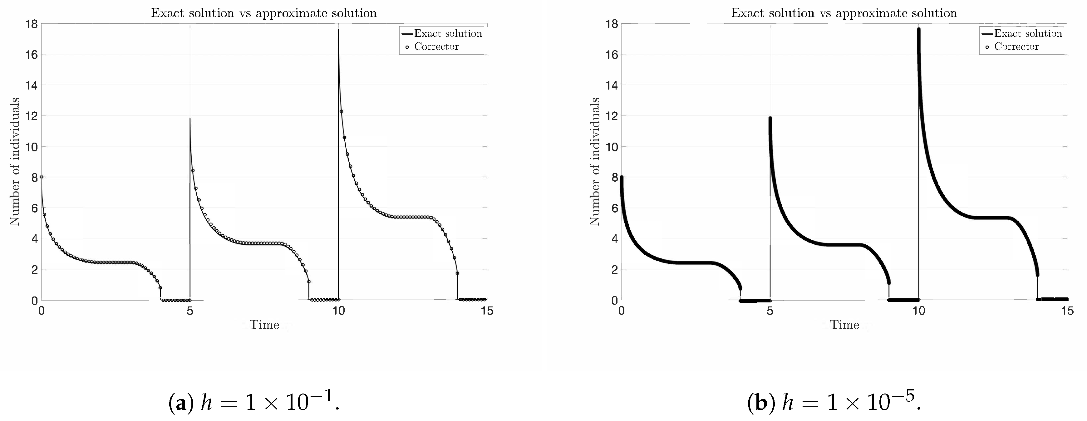
In order to validate the numerical method, we compared the numerical and the exact solution for the linear equation. We realize that the order of convergence that we obtained in the numerical experiments is higher than we proved in the theory. This fact may mean that it is possible to improve the estimates obtained under more stringent regularity assumptions regarding the functions involved.

We also compared the numerical and the exact solution of a realistic silkworm population model (118) based on a Stieltjes differential equation. We obtained a good behavior of the numerical method even though we approximated the right-hand side by a quadrature formula. The behavior observed in the solution of Equation (118) (0D model) can also be appreciated in the 2D model based on a parabolic partial differential equation of the Stieltjes type (cf. [13] (Section 5)):

$$\left\{\begin{array}{ll}{u}_g^{\prime }\left(t\right)-\nabla ·(\eta \nabla u)=f(t,u\left(t\right),u),\hfill & \mathrm{in}[(0,T)\backslash C_g]\times \Omega ,\\ \eta \nabla u·\mathbf{n}=0,\hfill & \mathrm{on}(0,T)\times \partial \Omega ,\\ u(0,x)=u_0\left(x\right),\hfill & \mathrm{in}\Omega ,\end{array}\right.$$

(130)

where $\Omega \subset {\mathbb{R}}^2$, $\eta >0$, $u_0\in L^2(\Omega )$, and f is given by Formula (119).

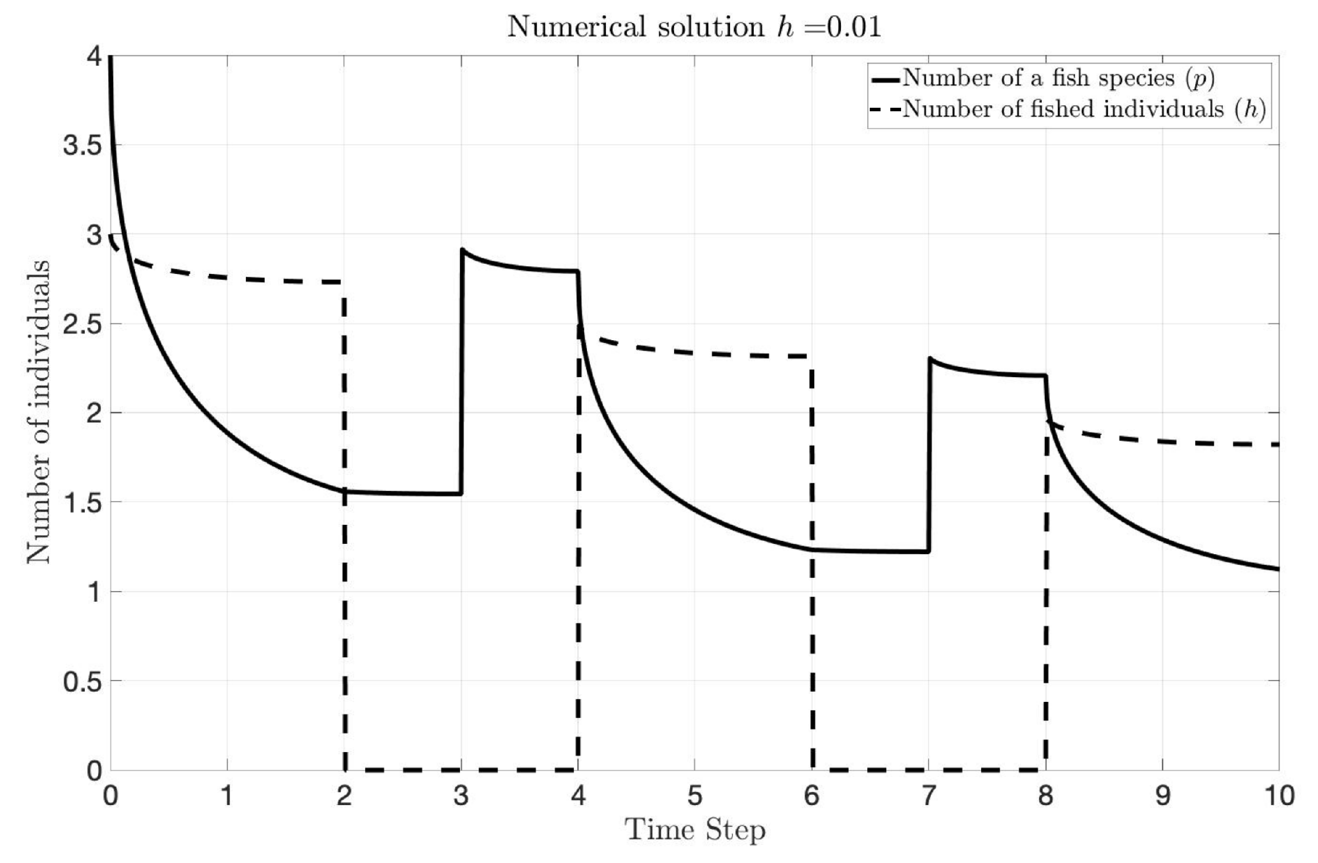
Finally, we proposed a numerical method to approximate the solution of systems of Stieltjes differential equations with several derivators, and we applied it to a system related to a fish population model for which no explicit solution is known. We observed that the behavior of the numerical solution is compatible with the interpretation of the model given in [12].

The ideas we developed in this work can be used to design an algorithm that improves the numerical approximation of the linear Stieltjes parabolic problems given in [13]. In this work, the authors obtained a numerical approximation of (130) by truncating the Fourier series of the solution and using the exact solution (120) to obtain each of the coefficients of the aforementioned series. Instead of truncating the Fourier series, we can perform a temporal discretization similar to the one that we developed in this work for Stieltjes differential equations. Indeed, if we assume Hypotheses 1–6 in the scalar case, we can consider the following modification of the approximation (53):

$$\begin{array}{ccc}\hfill {\displaystyle {\int }_{[t_k,t_{k+1})}{f}_{*}\left(x\right)\left(s\right)dg\left(s\right)}& \simeq & {\displaystyle f_{*}^C\left(x\right)\left(t_{k+1}\right)(g^C\left(t_{k+1}\right)-g^C\left(t_k\right))}\hfill \\ & & {\displaystyle +f_{*}\left(x\right)\left(t_k\right){\Delta }^{+}g\left(t_k\right)+{\Delta }^{+}{f}_{*}\left(x\right)\left(t_k\right)(g^C\left(t_{k+1}\right)-g^C\left(t_k\right)).}\hfill \end{array}$$

(131)

In this case, we obtain the following implicit numerical method: given $u_0=x_0$, we compute ${\left\{(u_{k-1}^{+},u_k)\right\}}_{k=1}^{N+1}$ as

$$\left\{\begin{array}{ccc}\hfill u_k^{+}& =& {\displaystyle u_k+f(t_k,u_k){\Delta }^{+}g\left(t_k\right),}\hfill \\ \hfill u_{k+1}& =& {\displaystyle u_k^{+}+f(t_{k+1},u_{k+1})(g\left(t_{k+1}\right)-g\left(t_k^{+}\right)).}\hfill \end{array}\right.$$

(132)

For example, if we follow the same scheme as in this work and consider the following linear Stieltjes parabolic problem:

$$\left\{\begin{array}{ll}{u}_g^{\prime }\left(t\right)-\nabla ·(\eta \nabla u)+\sigma u=f,\hfill & \mathrm{in}[(0,T)\backslash C_g]\times \Omega ,\\ \eta \nabla u·\mathbf{n}=0,\hfill & \mathrm{on}(0,T)\times \partial \Omega ,\\ u(0,x)=u_0\left(x\right),\hfill & \mathrm{in}\Omega ,\end{array}\right.$$

(133)

where $\Omega \subset {\mathbb{R}}^n$, $\eta ,\sigma >0$, $u_0\in {\mathcal{L}}^2(\Omega )$, and $f\in {\mathcal{L}}_g^2([0,T);L^2(\Omega ))$ (cf. [13] for a description of the Stieltjes–Bochner space ${\mathcal{L}}_g^2([0,T);L^2(\Omega ))$). We can apply Method (132) to the integral expression form of the solution of (133), and we obtain the following numerical method: given $u^0\in L^2(\Omega )$, we compute ${\left\{u_k\right\}}_{k=1}^{N+1}\subset H^1(\Omega )$ as

$$\begin{array}{c}{\displaystyle {\alpha }_{k+1}{\int }_{\Omega }{u}_{k+1}zdx+\eta {\int }_{\Omega }\nabla u_{k+1}·\nabla zdx+\sigma {\int }_{\Omega }{u}_{k+1}zdx={\int }_{\Omega }f\left(t_{k+1}\right)zdx}\hfill \\ {\displaystyle +{\alpha }_{k+1}{\int }_{\Omega }{u}_{k}zdx+{\alpha }_{k+1}{\Delta }^{+}g\left(t_k\right){\int }_{\Omega }f\left(t_k\right)zdx-{\alpha }_{k+1}{\Delta }^{+}g\left(t_k\right)\eta {\int }_{\Omega }\nabla u_k·\nabla zdx}\hfill \\ {\displaystyle -{\alpha }_{k+1}{\Delta }^{+}g\left(t_k\right)\sigma {\int }_{\Omega }{u}_{k}zdx,\forall z\in H^1(\Omega ),}\hfill \end{array}$$

(134)

where ${\alpha }_{k+1}={[g\left(t_{k+1}\right)-g\left(t_k^{+}\right)]}^{-1}$ (cf. [14] (Chapter 7) for the mathematical analysis of the previous approximation in the case $g\left(t\right)=t$). An analogous discretization can be applied to System (130), and the resulting scheme can be compared with the scheme given in [13]. In future works, we intend to mathematically study the approximation (134) even in the case of considering a finite-dimensional subspace $V_h\subset H^1(\Omega )$.