A New Log-Logistic Lifetime Model with Mathematical Properties, Copula, Modified Goodness-of-Fit Test for Validation and Real Data Modeling

Abstract

After defining a new log-logistic model and studying its properties, some new bivariate type versions using “Farlie-Gumbel-Morgenstern Copula”, “modified Farlie-Gumbel-Morgenstern Copula”, “Clayton Copula”, and “Renyi’s entropy Copula” are derived. Then, using the Bagdonavicius-Nikulin goodness-of-fit (BN-GOF) test for validation, we proposed a goodness-of-fit test for a new log-logistic model. The modified test is applied for the “right censored” real dataset of survival times. All elements of the modified test are explicitly derived and given. Three real data applications are presented for measuring the flexibility and the importance of the new model under the uncensored scheme. Two other real datasets are analyzed for censored validation.

1. Introduction

A new univariate version of the log-logistic (LL) model called the Rayleigh generalized log-logistic (RG-LL) distribution (see Equations (3) and (4) and their corresponding details) is introduced, studied, and checked in modeling censored and uncensored real datasets. Following the mathematical approach to the development of the RG-LL distribution, some new bivariate RG-LL type distributions using Farlie-Gumbel-Morgenstern (FGM) Copula ([1,2,3,4]), modified Farlie-Gumbel-Morgenstern Copula [5], Clayton Copula, and Renyi’s entropy Copula [6] are derived in this paper (see Section 3). Two major reasons as to why copulas are of interest to statisticians ([7]): “Firstly, as a way of studying scale-free measures of dependence; and secondly, as a starting point for constructing families of bivariate distributions.” Specifically, copulas are an important part of the study of dependence between two variables since they allow us to separate the effect of dependence from the effect of the marginal distributions. Further future articles could be allocated to study the new bivariate RG-LL type.

The new model is used for modeling three real datasets. The 1st data are an “engineering real-life data” and consist of 100 observations of “breaking stress of carbon fibers” given by [8]. The 2nd data are a “reliability survival data” and called the “survival times”, in days, of 72 guinea pigs infected with virulent tubercle bacilli, this data were originally observed and reported by [9]. The 3rd data are medical data and called leukemia data. This real dataset gives the survival times, in weeks, of 33 patients suffering from acute myelogenous leukemia. These applications are used to illustrate the importance, potentiality, and flexibility of the RG-LL model. The hazard rate function (HRF) of the 1st and 2nd real datasets is “monotonically increasing”. However, the HRF of the 3rd is “decreasing-constant-increasing”. These read datasets are analyzed by [10,11,12,13,14,15,16,17].

The RG-LL model has only three parameters. However, its competitive models have at least three parameters (or more) as illustrated in Section 5 (

Table A3. MLEs, SEs and CIs with $C_{\mathrm{AI}}$, $C_{\mathrm{Bayes}}$, $C_{\mathrm{HQ}}$ and $C_{\mathrm{CA}}$ for the breaking stress of carbon fibers data.

Model	$\widehat{\mathit{\theta }}$$, \widehat{{\mathit{a}}_{\mathbf{1}}}$$, \widehat{ {\mathit{a}}_{\mathbf{1}}}$$,\widehat{ \mathit{\beta }}$$,\widehat{ \mathit{\gamma }}$	${\mathit{C}}_{\mathbf{AI}}$$, {\mathit{C}}_{\mathbf{Bayes}}$$, {\mathit{C}}_{\mathbf{HQ}}$$\mathbf{and} {\mathit{C}}_{\mathbf{CA}}$
B XII	---, ---, 5.942, 0.1870, ---	382.94, 388.20, 383.010, 385.05
	---, ---, (1.28), (0.04), ---
	---, ---, (3.4,8.5), (0.1,0.3), ---
MOB XII	---, ---, 1.19,4.83,838.7	305.78, 313.60, 306.00, 308.96
	---, ---, (0.95), (4.89), (229.3)
	---, ---, (0, 3.1), (0,1.4), (389,1288)
TLB XII	---, ---, 1.35,1.06,13.73	323.50, 331.35, 323.78, 326.71
	---, ---, (0.38), (0.38), (8.4)
	---, ---, (0.6, 2.1), (0.3,1.8), (0, 30.2)
KwB XII	48.1, 79.5, 0.4, 2.7, ---	303.76, 314.21, 304.20, 308.00
	(19.34), (58.19), (0.1), (1.1), ---
	(10.1,86.0), (0,193.6), (0.16,0.5), (0.6,4.8), ---
BBXII	359.68, 260.1, 0.175, 1.12, ---	305.64, 316.06, 306.06, 309.85
	(57.9), (132.2), (0.013), (0.24), ---
	(246,473), (0.96,519), (0.14,0.2), (0.6,1.6), ---
BE BXII	0.38, 11.95, 0.94, 33.4, 1.71	305.81, 318.83, 306.50, 311.09
	(0.1), (4.6), (0.27), (6.3), (0.48)
	(0.2,0.5), (2.86,2), (0.4,1.5), (21,5), (0.8,2.6)
FKw BXII	0.54,4.22, 5.313, 0.41, 4.152	305.50, 318.55, 306.14, 310.80
	(0.14), (1.88), (2.32), (0.49), (1.99)
	(0.3, 0.8), (0.5,7.9), (0.9,9), (0, 1.7), (0.1,8)
ZB BXII	123.101, ---,0.368, 139.247, ---	302.96, 310.78, 303.21, 306.13
	(243.011), ---, (0.343), (318.546), ---
	(0, 599.40), ---, (0, 1.04), (0, 763.59), ---
RG-LL	2.504, 0.003, 0.739, ---, ---	302.75, 301.17, 299.18, 300.92
	(0.158), (0.000), (0.072), ---, ---
	(2.2, 2.8), ---, (0.56, 0.84), ---, ---

,

Table A4. MLEs, SEs, and CIs with $C_{\mathrm{AI}}$, $C_{\mathrm{Bayes}}$, $C_{\mathrm{HQ}}$ and $C_{\mathrm{CA}}$ for the survival times data.

Model	$\widehat{\mathit{\theta }}$$,\widehat{ {\mathit{a}}_{\mathbf{1}}}$$, \widehat{{\mathit{a}}_{\mathbf{1}}}$$,\widehat{ \mathit{\beta }}$$,\widehat{ \mathit{\gamma }}$	${\mathit{C}}_{\mathbf{AI}}$$, {\mathit{C}}_{\mathbf{Bayes}}$$, {\mathit{C}}_{\mathbf{HQ}}$$\mathbf{and} {\mathit{C}}_{\mathbf{CA}}$
B XII	---, ---, 3.102, 0.465, ---	209.6, 214.2, 209.77, 211.41
	---, ---, (0.538), (0.077), ---
	---, ---, (2.1, 4.2), (0.31, 0.6), ---
MO BXII	---, ---, 2.259, 1.533, 6.760	209.74, 216.61, 210.09, 212.44
	---, ---, (0.864), (0.907), (4.587)
	---, ---, (0.5, 3.95), (0, 3.3), (0, 15.8)
TL BXII	---, ---, 2.39, 0.458, 1.796	211.80, 218.63, 212.15, 214.51
	---, ---, (0.91), (0.24), (0.92)
	---, ---, (0.62,4.2), (0, 0.9), (0.002,3.6)
TL BXII	---, ---, 2.39, 0.458, 1.796	211.80, 218.62, 212.15, 214.53
	---, ---, (0.91), (0.244), (0.92)
	---, ---, (0.6,4.2), (0, 0.9), (0.002,3.6)
Kw BXII	14.11,7.42, 0.525, 2.274, ---	208.80, 217.86, 209.40, 212.40
	(10.81), (11.85), (0.28), (0.99), ---
	(0, 35.3), (0.30.65), (0, 1.1), (0.33, 4.2), ---
FBB XII	0.621, 0.549, 3.838, 1.381, 1.665	206.81, 218.20, 207.73, 211.31
	(0.54), (1.01), (2.79), (2.31), (0.44)
	(0, 1.7), (0, 2.5), (0, 9.3), (0, 6), (0.8, 4.5)
FKwB XII	0.558,0.31, 3.999, 2.131, 1.48	206.51, 217.90, 207.42, 211.01
	(0.44), (0.31), (2.08), (1.83), (0.36)
	(0, 1.4), (0, 0.9), (0, 3.1), (0, 5.7), (0.76, 2.2)
RG-LL	3.3, 0.004, 0.386, ---, ---	208.01, 211.11, 207.12, 209.53
	(0.24), (0.002), (0.041), ---, ---
	(2.8, 3.8), (0, 0.008), (0.32, 0.48), ---, ---

and

Table A5. MLEs, SEs, and CIs with $C_{\mathrm{AI}}$, $C_{\mathrm{Bayes}}$, $C_{\mathrm{HQ}}$ and $C_{\mathrm{CA}}$ for the leukemia data.

Model	$\widehat{\mathit{\theta }}$$,\widehat{ {\mathit{a}}_{\mathbf{1}}}$$, \widehat{{\mathit{a}}_{\mathbf{1}}}$$,\widehat{ \mathit{\beta }}$$,\widehat{ \mathit{\gamma }}$	${\mathit{C}}_{\mathbf{AI}}$$, {\mathit{C}}_{\mathbf{Bayes}}$$, {\mathit{C}}_{\mathbf{HQ}}$$\mathbf{and} {\mathit{C}}_{\mathbf{CA}}$
B XII	---, ---, 58.7, 0.006, ---	328.21, 331.19, 328.61, 329.20
	---, ---, (42.4), (0.004), ---
	---, ---, (0, 141.8), (0, 0.01), ---
MOB XII	---, ---, 11.838, 0.078, 12.25	315.54, 320.01, 316.38, 317.04
	---, ---, (4.368), (0.013), (7.77)
	---, ---, (0, 141.8), (0, 0.01), (0, 27.5)
TLB XII	---, ---,0.281, 1.882, 50.215	316.30, 320.73, 317.09, 317.76
	---, ---, (0.29), (2.4), (176.5)
	---, ---, (0, 0.9), (0, 6.6), (0, 396.2)
KwB XII	9.201, 36.428, 0.242, 0.941, ---	317.36, 323.31, 318.79, 319.33
	(10.1), (35.7), (0.167), (1.06), ---
	(0, 28.9), (0, 106), (0, 0.6), (0, 3), ---
BB XII	96.10, 52.12, 0.10, 1.23, ---	316.50, 322.45, 317.89, 318.50
	(41.20), (33.49), (0.02), (0.34), ---
	(15, 176.8), (0, 117.8), (0.6, 0.15), (0.6, 1.9), ---
BEB XII	0.087, 5.007, 1.561, 31.270, 0.318	317.58, 325.10, 319.8, 320.10
	(0.08), (3.851), (0.01), (12.9), (0.03)
	(0, 0.3), (0, 13), (1.5, 2), (5.9, 57), (0.3, 0.4)
FBB XII	15.19, 32.5, 0.23, 0.58, 21.86	317.87, 325.36, 320.08, 320.37
	(11.6), (9.87), (0.09), (0.07), (35.55)
	(0, 38), (12.7, 51), (0.05, 0.4), (0.45, 1), (0, 92)
FKwB XII	14.7, 15.285, 0.29, 0.84, 0.03	317.76, 325.2, 319.98, 320.27
	(12.39), (18.87), (0.22), (0.85), (0.08)
	(0, 39), (0, 52.3), (0, 0.7), (0, 2.5), (0, 0.2)
ZBB XII	41.97, ---,0.16, 44.26, ---	313.85, 318.35, 314.40, 315.40
	(38.79), ---, (0.08), (47.65), ---
	(0, 118), ---, (0, 0.3,) (0, 138), ---
RG-LL	0.8, 0.068, 0.487, ---, ---	313.44, 316.41, 313.11, 313.02
	(0.148), (0.033), (0.089), ---, ---
	(0.50, 1.1), (0, 0.12), (0.32, 0.68), ---, ---

). It is worth mentioning that, the lifetime model with a smaller number of parameters is a favorable one especially when if it gives a better (or same) fit. The RG-LL model has the lowest (best) value of the used criteria (see Table A3, Table A4 and Table A5). Therefore, it is recommended to apply the RG-LL model in modeling instead of all the other competitive models. For the applied purposes, especially in the mathematical modeling, the RG-LL model could be useful in the following applied cases:

• Modeling the “asymmetric monotonically right skewed” heavy tail data sets (see second and third applications).
• Modeling the “asymmetric monotonically right skewed” heavy tail data sets for the first time ever (see [18]).
• In the engineering field, the RG-LL distribution can be applied for modeling the “breaking stress data” which have “monotonically increasing” HRF. As shown in Table A3, the RG-LL model proved its superiority against many competitive models.
• In “survival analysis”, the RG-LL distribution could be chosen for modeling the “survival times data” which have a “monotonically increasing” HRF as illustrated in Table A4.
• In the medical field, the RG-LL distribution could be considered in modeling the “leukemia data” which have “decreasing-constant-increasing” HRF (see Table A5).

For these reasons, we are motivated to introduce and study the RG-LL distribution.

For simulation purposes, the algorithm of “Barzilai-Borwein” (BB) (see [19]) is used via a simulation study for assessing the performance of the estimators with different sample sizes as the sample size tends to $\infty$ (for more details, see [20,21,22]). For validation purposes and using the BN-GOF test under the right censored data, we propose a modified chi-square GOF test for the RG-LL model. Based on the maximum likelihood estimators (MLEs) on initial data, the modified BN-GOF test recovers the loss in information while grouping data and follow chi-square distributions. All elements of the modified BN-GOF criteria tests are explicitly derived and given (for more details see [20,23,24]).

Generally, the LL distribution is a continuous model for a non-negative random variables (RVs). It is used in survival analysis as a parametric model for events whose rate increases initially and decreases later such as mortality rate from cancer following diagnosis or treatment (for more details see [25,26,27,28,29,30,31]). The LL model has also been used in hydrology in modeling stream flow and precipitation. In economics, the LL is employed as a simple distribution of the distribution of wealth or income. A RV $Z$ is said to have the one parameter LL distribution if its cumulative distribution functions (CDF) can be written as:

$$G_{a_2}\left(z\right){|}_{\left(z>0,a_2>0\right)}=1-\frac{1}{1+z^{a_2}}$$

(1)

here $a_2>0$ refers to the shape parameter. A scale and location parameter can be introduced in many ways to make (1) a three-parameter distribution. It is worth mentioning that the model in (1) is a member of the Pareto Type I distribution. The corresponding probability density function (PDF) of (1) is given by

$$g_{a_2}\left(z\right)=a_2\frac{z^{a_2-1}}{{\left(1+z^{a_2}\right)}^2}.$$

(2)

The PDF in (2) is a special member from the well-known Burr type XII (BXII) model (see [25,26,27,28,29,30,31]). Based on the family of [15] and using (1), the CDF of the Rayleigh generalized LL (RG-LL) is defined by

$$F_{\theta ,a_1,a_2}\left(z\right){|}_{\left(z,\theta ,a_1,a_2>0\right)}=1-exp\left\{-a_1{\left[{\left(1+z^{a_2}\right)}^{\theta }-1\right]}^2\right\}$$

(3)

the corresponding PDF to (3) is given as

$$f_{\theta ,a_1,a_2}\left(z\right){|}_{\left(z,\theta ,a_1,a_2>0\right)}=2\theta a_1{a}_2\frac{z^{a_2-1}{\left(1+z^{a_2}\right)}^{\theta -1}\left[{\left(1+z^{a_2}\right)}^{\theta }-1\right]}{exp\left\{a_1{\left[{\left(1+z^{a_2}\right)}^{\theta }-1\right]}^2\right\}}$$

(4)

For $a_1=1,$ the RG-LL model reduces to the two parameter RG-LL model. For $\theta =1,$ the RG-LL model reduces to the R-LL model (with three parameters). For $\theta =a_1=1,$ the RG-LL model reduces to the R-LL model (with two parameters). The HRF can be derived from $h_{\theta ,a_1,a_2}\left(z\right)=\frac{f_{\theta ,a_1,a_2}\left(z\right)}{1-F_{\theta ,a_1,a_2}\left(z\right)}$. Let $ℬ=inf\left\{z|G_{a_2}\left(z\right)>0\right\}$, the asymptotics of the CDF, PDF, and HRF as $z\to ℬ$ are given by

$$\begin{gathered} F_{\theta ,a_1,a_2}\left(z\right) {|}_{\left(z\to ℬ,a_1=1\right)}\sim {\theta }^2{\left(1-\frac{1}{1+z^{a_2}}\right)}^2, \\ {f}_{\theta ,a_1,a_2}\left(z\right) {|}_{\left(z\to ℬ,a_1=1\right)}\sim 2a_2{\theta }^2\frac{z^{a_2-1}}{{\left(1+z^{a_2}\right)}^2}\left[1-\frac{1}{1+z^{a_2}}\right], \end{gathered}$$

and

$$h_{\theta ,a_1,a_2}\left(z\right) {|}_{\left(z\to ℬ,a_1=1\right)}\sim 2a_2{\theta }^2\frac{z^{a_2-1}}{{\left(1+z^{a_2}\right)}^2}\left(1-\frac{1}{1+z^{a_2}}\right).$$

The asymptotics of CDF, PDF and HRF as $z\to \infty$ are derived by

$$\begin{gathered} 1-F_{\theta ,a_1,a_2}\left(z\right) {|}_{\left(z\to \infty ,a_1=1\right)}\sim exp\left[-{\left(\frac{1}{1+z^{a_2}}\right)}^{-2\theta }\right] \\ {f}_{\theta ,a_1,a_2}\left(z\right) {|}_{\left(z\to \infty \right),a_1=1}\sim 2a_2\theta \frac{z^{a_2-1}}{{\left(1+z^{a_2}\right)}^2}{\left(\frac{1}{1+z^{a_2}}\right)}^{-2\theta -1}exp\left[-{\left(\frac{1}{1+z^{a_2}}\right)}^{-2\theta }\right] \end{gathered}$$

and

$$h_{\theta ,a_1,a_2}\left(z\right) {|}_{\left(z\to \infty ,a_1=1\right)}\sim 2a_2\theta \frac{z^{a_2-1}}{{\left(1+z^{a_2}\right)}^2}{\left[\frac{1}{1+z^{a_2}}\right]}^{-2\theta -1}$$

Figure 1 gives some plots of PDF and HRF for the RG-LL model. From Figure 1 (left panel), we conclude that the proposed PDF of the RG-LL model can be “uniform”, “unimodal”, “symmetric” or “asymmetric left skewed” (or asymmetric right skewed (see

Table A1. Numerical results for ${\mu }_1^{\prime }$, Var($Z$), Ske($Z$), Kur($Z$) for the RG-LL model.

$\mathit{\theta }$	${\mathit{a}}_{\mathbf{1}}$	${\mathit{a}}_{\mathbf{2}}$	${\mathit{\mu }}_{\mathbf{1}}^{\prime }$	$\mathbf{Var}\left(\mathit{Z}\right)$	$\mathbf{Ske}\left(\mathit{Z}\right)$	$\mathbf{Kur}\left(\mathit{Z}\right)$
0.1	10	3	2.3014850	1.07723700	1.2469570	5.644436
0.25			1.1656230	0.09155918	0.1903485	2.984291
0.5			0.8348619	0.03179571	−0.1816630	2.910675
1			0.6320478	0.01499990	−0.3732641	3.035430
5			0.3565924	0.00409134	−0.5292522	3.217301
7.5			0.3106052	0.00306466	−0.5423596	3.235840
10			0.2817936	0.00250640	−0.5489192	3.244724
12.5			0.2613663	0.00214794	−0.5528574	3.251049
15			0.2458125	0.00189505	−0.5554835	3.258577
3.5	0.00001	1.5	2.4439090	0.126387700	−0.7106222	3.773512
	0.001		1.3234170	0.058929280	−0.686609	3.627384
	0.1		0.5704622	0.022007440	−0.4085326	2.92692
	0.5		0.3889885	0.012877710	−0.2505082	2.728826
	1		0.3246634	0.009765043	−0.1830979	2.678376
	5		0.2064316	0.004609066	−0.04542067	2.635436
	10		0.1678268	0.003197180	0.0019725	2.639189
	50		0.1017226	0.001267371	0.0816486	2.667219
	100		0.08148813	0.000830205	0.1043870	2.674599
	500		0.04827376	0.000300035	0.1378587	16.01191
	1000		0.03843619	0.000191606	−3.7303240	35.06832
	2000		0.03057584	0.000121892	−0.1520501	−8.218386
	5000		0.02257409	6.675676 × 10⁻⁵	7.694268	−35.06735
	10000		0.01793546	4.224229 × 10⁻⁵	−13.52702	110.2359
	20000		0.01424575	2.669551 × 10⁻⁵	−10.83246	62.76824
	50000		0.01050316	1.453355 × 10⁻⁵	22.28915	−174.8386
2	10	0.1	1.662079 × 10⁻¹⁰	3.56035 × 10⁻¹³	3601.587	13223681
		0.5	0.0209009	0.0003730464	1.688587	6.977619
		1	0.1296743	0.0040855080	0.4852051	2.948691
		5	0.6492678	0.0055586940	−0.7296955	3.751450
		6	0.6970608	0.0045386420	−0.8017811	3.969663

)). From Figure 1 (right panel), the HRF can be “asymmetric monotonically increasing” ($\theta =0.95,a_1=0.01,a_2=1.5$) or “decreasing-constant” ($\theta =1.5,a_1=0.01,a_2=0.35$) or “J shaped” ($\theta =1,a_1=1,a_2=20$) or “constant” ($\theta =1.5,a_1=0.1,a_2=0.45$).

The rest of the paper is organized as follows. In Section 2, some mathematical properties of the new model are derived. In Section 3, some new bivariate type versions using “Farlie-Gumbel-Morgenstern Copula”, “modified Farlie-Gumbel-Morgenstern Copula”, “Clayton Copula” and “Renyi’s entropy Copula” are obtained. In Section 4, we provided three applications to real data to illustrate the flexibility of the new model. The modified BN-GOF test is presented and applied in Section 5. Simulation experiments under censorship for assessing the new test are performed in Section 6. Censored validation under real data is considered in Section 7. Finally, some concluding remarks are addressed in Section 8.

2. Properties

2.1. Moments and Generating Function

The PDF of the RG-LL model in (4) can be expressed as:

$$F\left(z\right)=1-\underset{A_{a_1,a_{2,}\theta }\left(z\right)}{\underbrace{exp\left\{-a_1{\left[\frac{1-{\left(\frac{1}{1+z^{a_2}}\right)}^{\theta }}{{\left(\frac{1}{1+z^{a_2}}\right)}^{\theta }}\right]}^2\right\}}}.$$

Expanding $A_{a_1,a_{2,}\theta }\left(z\right)$ using the power series, we get:

$$F\left(z\right)=1-{\displaystyle \sum }_{i_i=0}^{\infty } \frac{{\left(-a_1\right)}^{i_1}}{i_1!}\underset{B_{a_{2,}\theta ,2i_1}\left(z\right)}{\underbrace{{\left[1-{\left(\frac{1}{1+z^{a_2}}\right)}^{\theta }\right]}^{2i_1}}}{\left(\frac{1}{1+z^{a_2}}\right)}^{-\theta 2i_1}.$$

Applying the generalized binomial expansion to the quantity $B_{a_{2,}\theta ,2i_1}\left(z\right)$, we have

$$F\left(z\right)=1-{\displaystyle \sum }_{i_1,i_2=0}^{\infty } \frac{{\left(-a_1\right)}^{i_1+i_2}}{i_1!}\left(\begin{array}{c}2i_1\\ i_2\end{array}\right)\underset{C_{a_{2,}\theta \left(i_2-2i_1\right)}\left(z\right)}{\underbrace{{\left(\frac{1}{1+z^{a_2}}\right)}^{\theta \left(i_2-2i_1\right)}}}.$$

Again, applying the generalized binomial expansion to the quantity $C_{a_{2,}\theta \left(i_2-2i_1\right)}\left(z\right)$, we arrive at

$$F\left(z\right)=1-{\displaystyle \sum }_{i_3=0}^{\infty } q_{i_3}{\left[G_{a_2}\left(z\right)\right]}^{i_3},$$

where $q_{i_3}={{\displaystyle \sum }}_{i_1,i_2=0}^{\infty } \frac{{\left(-a_1\right)}^{i_1+i_2+i_3}}{i_1!}\left(\begin{array}{c}2i_1\\ i_2\end{array}\right)\left(\begin{array}{c}\theta \left(i_2-2i_1\right)\\ i_3\end{array}\right)$ and ${\left[G_{a_2}\left(z\right)\right]}^{i_3}={\left[1-\frac{1}{1+z^{a_2}}\right]}^{i_3}$ is the CDF of the exponentiated LL (Exp-LL) model. By differentiating the last equation, we get

$$f\left(z\right)={\displaystyle \sum }_{i_4=0}^{\infty }{{\rm Y}}_{\left[i_4\right]} g_{a_2,\left(1+i_4\right)}\left(z\right),$$

(5)

where ${{\rm Y}}_{\left[i_4\right]}=-b_{\left[i_4\right]}$ and $b_{\left[i_4\right]}\hspace{0.17em}={{\displaystyle \sum }}_{i_1,i_2,i_3=0}^{\infty }\frac{{\left(-1\right)}^{i_1+i_2+i_3+i_4}}{i_1!i_4!}\left(\begin{array}{c}2i_1\\ i_2\end{array}\right)\left(\begin{array}{c}\theta \left(i_2-2i_1\right)\\ i_3\end{array}\right)\left(\begin{array}{c}1+i_3\\ i_4\end{array}\right),$ the PDF

$$g_{a_2,\left(1+i_4\right)}\left(z\right)=\left(1+i_4\right)a_2{z}^{a_2-1}{\left(1+z^{a_2}\right)}^{-2-i_4}$$

(6)

is the LL PDF with parameters $a_2$ and $\left(1+i_4\right)$. Similarly, the CDF (2) of RG-LL can be re-expressed as $F\left(z\right)={{\displaystyle \sum }}_{i_4=0}^{\infty }{{\rm Y}}_{\left[i_4\right]}{G}_{a_2,\left(1+i_4\right)}\left(z\right),$ where $G_{a_2,\left(1+i_4\right)}\left(z\right)=1-{\left(1+z^{a_2}\right)}^{-1-i_4}$ is the CDF of the LL model with parameters $a_2$ and $\left(1+i_4\right)$. In terms of beta function of the second type, $B\left(a_1,a_2\right)$, where $B\left(a_1,a_2\right)={{\displaystyle \int }}_0^{\infty }{t}^{a_1-1}{(1+t)}^{-\left(a_1+a_2\right)}dt$, the $p^{th}$ ordinary moment of $Z$ can be expressed as (see [10,11,16,32,33,34]):

$${\mu }_p^{\prime }{|}_{\left(p<\left(1+i_4\right)a_2\right)}={\displaystyle \sum }_{i_4=0}^{\infty }{{\rm Y}}_{\left[i_4\right]}\left(1+i_4\right) B\left(1+\frac{p}{a_2},\left(1+i_4\right)-\frac{p}{a_2}\right),$$

(7)

By setting $p=1$ in (7), we get the mean of $Z$. Similarly, in terms of incomplete beta function of the second type, $B\left(q;a_1,a_2\right)$, where $B\left(q;a_1,a_2\right)={{\displaystyle \int }}_0^q{t}^{a_1-1}{(1+t)}^{-\left(a_1+a_2\right)}dt$, the $p^{th}$ incomplete moment of $Z$ can be written as:

$$I_p\left(t\right){|}_{\left(p<\left(1+i_4\right)a_2\right)}={\displaystyle \sum }_{i_4=0}^{\infty }{{\rm Y}}_{\left[i_4\right]}\left(1+i_4\right) B\left(t^{a_2};1+\frac{p}{a_2},\left(1+i_4\right)-\frac{p}{a_2}\right),$$

The moment generating function (MGF) $M_z\left(t\right)=E\left(exp\left(tz\right)\right)$ of $z$ can be derived from (5) as

$$M_z\left(t\right)={\displaystyle \sum }_{i_4,p=0}^{\infty }{{\rm Y}}_{\left[i_4\right]}\left(1+i_4\right) B\left(1+\frac{p}{a_2},\left(1+i_4\right)-\frac{p}{a_2}\right){|}_{\left(p<\left(1+i_4\right)a_2\right)}.$$

2.2. Probability Weighted Moments (PWMs)

The ${(p,q)}^{th}$ PWM of $Z$ following the RG-LL model, say $m_{p,q}$, is formally defined by $m_{p,q}=E\left\{z^{p}F{(z)}^q\right\}.$ The ${(p,q)}^{th}$ PWM of $Z$ can be expressed as:

$$m_{p,q}={\displaystyle \sum }_{q=0}^{\infty }{{\rm Y}}_{\left[q\right]}\left(1+q\right) B\left(\frac{p}{a_2}+1,\left(1+q\right)-\frac{p}{a_2}\right){|}_{\left(p<\left(1+q\right)a_2\right)},$$

where

$${{\rm Y}}_{\left[q\right]}=2\theta a_1{\displaystyle {\displaystyle \sum }_{i,i_1,i_2,i_3=0}^{\infty }}\frac{{\left(-1\right)}^{i+i_1+i_2+i_3}{\left(1+i\right)}^{i_1}}{\Gamma \left(1+q\right)\Gamma \left(1+i_1\right)!}{\left(q\right)}_{i_3}\left(\begin{array}{c}1+i_3\\ r\end{array}\right)\left(\begin{array}{c}\left(1+i_1\right)2-1\\ i_2\end{array}\right)\left(\begin{array}{c}\theta \left[-\left(1+i_1\right)2+i_2\right]-1\\ i_3\end{array}\right),$$

and ${\left(a_1\right)}_{a_2}=a_1\left(a_1-1\right)\dots \left(1+a_1-a_2\right)$ is the “descending factorial” and $a_2$ is a positive integer.

2.3. Moment of the Reversed Residual Life

The $p^{th}$ moment of the reversed residual life, say $A_p\left(t\right)=E\left[{(t-z)}^p\hspace{0.17em}{|}_{\left(z\le t, t>0,p=1,2,\dots \right)}\right].$ Then, we have $A_p\left(t\right)=F^{-1}\left(t\right){{\displaystyle \int }}_0^t{(t-z)}^{p}dF\left(z\right).$ Then, the $p^{th}$ moment of the reversed residual life of $Z$ becomes

$$A_p\left(t\right)=F^{-1}\left(t\right){\displaystyle \sum }_{r=0}^{\infty }{{\rm Y}}_{\left[i_4\right]}^{*}\left(1+i_4\right) B\left(t^{a_2};\left(1+i_4\right)-\frac{p}{a_2},1+\frac{p}{a_2}\right),$$

where ${{\rm Y}}_{\left[i_4\right]}^{*}={{\rm Y}}_{\left[i_4\right]}{\displaystyle \underset{r=0}{\overset{p}{{\displaystyle \sum } }}}\left(\begin{array}{c}p\\ r\end{array}\right){\left(-1\right)}^r{t}^{p-r}.$

2.4. Numerical Analysis for Skewness and Kurtosis

The effects of the three parameters for the RG-LL model on the mean (${\mu }_1^{\prime }$), variance (Var(Z)), skewness (Ske(Z)), and kurtosis (Kur(Z)) are listed in Table A1 (see the Appendix A). The effects of the parameter a₂ for the standard LL model on the ${\mu }_1^{\prime }$, Var(Z), Ske(Z), and Kur(Z) are listed in

Table A2. Numerical results for ${\mu }_1^{\prime }$, Var($Z$), Ske($Z$), Kur($Z$) for the RG-LL model.

${\mathit{a}}_{\mathbf{2}}$	${\mathit{\mu }}_{\mathbf{1}}^{\prime }$	$\mathbf{Var}\left(\mathit{Z}\right)$	$\mathbf{Ske}\left(\mathit{Z}\right)$	$\mathbf{Kur}\left(\mathit{Z}\right)$
5.00	1.068959	0.17863230	2.48528	29.5562
7.50	1.029853	0.06671700	1.33004	9.18867
10.0	1.016641	0.03540090	0.93667	6.51021
12.5	1.010606	0.02206170	0.72919	5.56385
15.0	1.007348	0.01510236	0.59899	5.10838
17.5	1.005391	0.01100040	0.50908	4.85121
20.0	1.004124	0.00837532	0.44302	4.69083
25.0	1.002637	0.00532522	0.35216	4.50848
30.0	1.001830	0.00368497	0.29246	4.41214
35.0	1.001344	0.00270154	0.25017	4.35495
40.0	1.001029	0.00206550	0.21860	4.31819
45.0	1.000813	0.00163045	0.19414	4.29314
50.0	1.000658	0.00131982	0.17299	4.33383
55.0	1.000544	0.00109017	0.15866	4.26215
60.0	1.000457	0.00091569	0.14538	4.25213
65.0	1.000389	0.00078000	0.13416	4.24442
70.0	1.000336	0.00067239	0.12455	4.23827
75.0	1.000292	0.00058562	0.11623	4.23332
80.0	1.000257	0.00051462	0.10895	4.22928
85.0	1.000228	0.00045580	0.10253	4.22593
90.0	1.000203	0.00040652	0.09682	4.22313
95.0	1.000182	0.00036482	0.09171	4.22077
100	1.000164	0.00032925	0.08717	3.74092

(see the Appendix A). From Table A1 and Table A2 we note that, the new additional shape parameters θ and a₁ have an effect on ${\mu }_1^{\prime }$, Var(Z), Ske(Z), and Kur(Z). For the RG-LL model, Ske(Z) can range in the interval (−10.8325, 3601.587). However, for the LL model, Ske(Z) can range in the interval (0.087169, 2.485276). Therefore, the new model can be left skewed and also right skewed, however, the LL model can only be right skewed. For the RG-LL model, Kur(Z) can range in the interval (−174.8386, 13223681). However, for the LL model, Kur(Z) can range only in the interval (3.7409, 29.5562).

3. Copula

3.1. Bivariate RG-LL Using FGM Copula

First, we start with CDF for the FGM family (see [1,2,3,4]) of two random variables $\left(Z_1,Z_2\right)$ which has the following form $F_{\mathit{\phi }}\left(z_1,z_2\right){|}_{\left(|\mathit{\phi }|\le 1\right)}=uw\left(1+\mathit{\phi }{u}^{*}{w}^{*}\right).$ Let $u^{*}=\left(1-u\right)\in \left(0,1\right)$ and $w^{*}=\left(1-w\right)\in \left(0,1\right).$ Setting $u^{*}=1-F_1\left(z_1\right)$ and $w^{*}=1-F_2\left(z_2\right)$ where $u^{*}=exp\left\{-a_1{\left[{\left(1+z_1^{a_2}\right)}^{{\theta }_1}-1\right]}^2\right\},$ and $w^{*}=exp\left\{-b_1{\left[{\left(1+z_2^{b_2}\right)}^{{\theta }_2}-1\right]}^2\right\}.$

3.2. Via Clayton Copula

The Bivariate Extension

The bivariate extension via Clayton Copula can be considered as a weighted version of the Clayton Copula which is in the form $C\left(u,v\right)={\left[u^{-\mathit{\phi }}+v^{-\mathit{\phi }}-1\right]}^{-\frac{1}{\mathit{\phi }}}.$ Let us assume that $X\sim$ RG-LL $\left({\theta }_1,a_1,a_2\right)$ and $Z\sim$ RG-LL $\left({\theta }_2,b_1,b_2\right).$ Then, setting $u=u_{{\theta }_1,a_1,a_2}\left(x\right)=F_1$ and $v=v_{{\theta }_2,b_1,b_2}\left(z\right)=F_2,$ the associated CDF of the bivariate RG-LL type distribution will be:

$$H\left(x,z\right)={\left\{\begin{array}{c}{\left(1-exp\left\{-a_1{\left[{\left(1+x^{a_2}\right)}^{{\theta }_1}-1\right]}^2\right\}\right)}^{-\mathit{\phi }}\\ +{\left(1-exp\left\{-b_1{\left[{\left(1+z^{b_2}\right)}^{{\theta }_2}-1\right]}^2\right\}\right)}^{-\mathit{\phi }}\\ -1\end{array}\right\}}^{-\frac{1}{\mathit{\phi }}}.$$

The “$m$-dimensional extension” can be written as:

$$H\left(z_i\right)={\left[{\displaystyle \sum }_{i=1}^m{\left(1-exp\left\{-a_i{\left[{\left(1+z_i^{a_i}\right)}^{{\theta }_i}-1\right]}^2\right\}\right)}^{-\mathit{\phi }}+1-m\right]}^{-\frac{1}{\mathit{\phi }}},$$

where $z_i=z_1,z_2,\cdots ,z_m.$

3.3. Bivariate RG-LL Type via Modified FGM Copula

Following [5], the (joint CDF) J-CDF of the bivariate modified FGM copula can be expressed as $C_{\epsilon }\left(u,w\right)=uw+\epsilon \widetilde{\mathsf{\vartheta }\left(u\right)}\widetilde{\mathsf{\phi }\left(w\right)},$ where $\widetilde{\mathsf{\vartheta }\left(u\right)}=u\overline{\mathsf{\vartheta }\left(u\right)}$, and $\widetilde{\mathsf{\phi }\left(w\right)}=w\overline{\mathsf{\phi }\left(w\right)}$. Here $\mathsf{\vartheta }\left(u\right)$ and $\mathsf{\phi }\left(w\right)$ are two absolutely continuous functions on $\left(0,1\right)$ with the following conditions: (I)-The “boundary” condition: $0=\mathsf{\vartheta }\left(1\right)=\mathsf{\vartheta }\left(0\right)=\mathsf{\phi }\left(1\right)=\mathsf{\phi }\left(0\right).$ (II)-Let

$${ℒ}_1=inf\left\{\frac{\partial }{\partial u}\widetilde{\mathsf{\vartheta }\left(u\right)}|{\mathcal{C}}_1\left(u\right)\right\}<0,{\mathscr{H}}_1=sup\left\{\frac{\partial }{\partial u}\widetilde{\mathsf{\vartheta }\left(u\right)}|{\mathcal{C}}_1\left(u\right)\right\}<0,$$

$${ℒ}_2=inf\left\{\frac{\partial }{\partial w}\widetilde{\mathsf{\phi }\left(w\right)}|{\mathcal{C}}_2\left(w\right)\right\}>0,{\mathscr{H}}_2=sup\left\{\frac{\partial }{\partial w}\widetilde{\mathsf{\phi }\left(w\right)}|{\mathcal{C}}_2\left(w\right)\right\}>0.$$

Then, $1\le min\left({ℒ}_1{\mathscr{H}}_1,{ℒ}_2{\mathscr{H}}_2\right)\le \infty ,$ where

$$\frac{\partial }{\partial u}\widetilde{\mathsf{\vartheta }\left(u\right)}=\mathsf{\vartheta }\left(u\right)+u\frac{\partial }{\partial u}\mathsf{\vartheta }\left(u\right),$$

$${\mathcal{C}}_1\left(u\right)=\left\{u:u\in \left(0,1\right) | \frac{\partial }{\partial u}\widetilde{\mathsf{\vartheta }\left(u\right)} \mathrm{exists}\right\},$$

and

$${\mathcal{C}}_2\left(w\right)=\left\{w:w\in \left(0,1\right) | \frac{\partial }{\partial w}\widetilde{\mathsf{\vartheta }\left(w\right)} \mathrm{exists}\right\}.$$

3.3.1. Bivariate RG-LL-FGM (Type-I) Model

Here, we consider the following functional form for both $\mathsf{\vartheta }\left(u\right)$ and $\mathsf{\phi }\left(w\right)$ as

$$C_{\epsilon }\left(u,w\right)=\left[\begin{array}{c}\left(1-exp\left\{-a_1{\left[{\left(1+u^{a_2}\right)}^{{\theta }_1}-1\right]}^2\right\}\right)\\ \times \left(1-exp\left\{-b_1{\left[{\left(1+w^{b_2}\right)}^{{\theta }_2}-1\right]}^2\right\}\right)\end{array}\right]+\epsilon \left[\widetilde{\mathsf{\vartheta }\left(u\right)}\widetilde{\mathsf{\phi }\left(w\right)} \right],$$

where

$$\widetilde{\mathsf{\vartheta }\left(u\right)}\frac{1}{u}=exp\left\{-a_1{\left[{\left(1+u^{a_2}\right)}^{{\theta }_1}-1\right]}^2\right\}{|}_{{\theta }_1,a_1,a_2>0},$$

and

$$\widetilde{\mathsf{\phi }\left(w\right)}\frac{1}{v} =exp\left\{-b_1{\left[{\left(1+w^{b_2}\right)}^{{\theta }_2}-1\right]}^2\right\}{|}_{{\theta }_2,b_1,b_2>0}.$$

3.3.2. Bivariate RG-LL-FGM (Type-II) Model

Consider the following functional form for both ϑ(u) and φ(w) which satisfy all the conditions stated earlier where $\mathsf{\vartheta }\left(u\right){|}_{\left({\epsilon }_1>0\right)}=u^{{\epsilon }_1}{\left(1-u\right)}^{1-{\epsilon }_1} \mathrm{and} \mathsf{\phi }\left(w\right){|}_{\left({\epsilon }_2>0\right)}=v^{{\epsilon }_2}{\left(1-w\right)}^{1-{\epsilon }_2}.$

The corresponding bivariate RG-LL-FGM (Type-II) copula can be derived from:

$$C_{\epsilon ,{\epsilon }_1,{\epsilon }_2}\left(u,w\right)=uw\left[1+\epsilon u^{{\epsilon }_1}{w}^{{\epsilon }_2}{\left(1-u\right)}^{1-{\epsilon }_1}{\left(1-w\right)}^{1-{\epsilon }_2}\right].$$

3.3.3. Bivariate RG-LL-FGM (Type-III) Model

Consider the following functional form for both $\mathsf{\vartheta }\left(u\right)$ and $\mathsf{\phi }\left(w\right)$ which satisfy all the conditions stated earlier where $\mathsf{\vartheta }\left(u\right)=u\left[\log \left(1+\overline{u}\right)\right] \mathrm{and} \mathsf{\phi }\left(w\right)=w\left[\log \left(1+\overline{w}\right)\right].$

In this case, one can also derive a closed form expression for the associated CDF of the bivariate RG-LL-FGM (Type-III).

3.3.4. Bivariate RG-LL-FGM (Type IV) Model

The J-CDF of the bivariate RG-LL-FGM (Type-IV) model can be derived from $C\left(u,w\right)=u{F}^{-1}\left(w\right)+w{F}^{-1}\left(u\right)-F^{-1}\left(u\right)F^{-1}\left(w\right).$

3.4. Bivariate RG-LL Type Using Renyi’s Entropy Copula

Due to [6], The J-CDF of the Renyi’s entropy Copula can be expressed as $C\left(u,w\right)=z_{2}u+z_{1}w-z_1{z}_2,$ then, the associated bivariate MOLBX will be

$$\begin{gathered} C\left(z_1,z_2\right)=C\left(F_{{\underset{\_}{V}}_1}\left(y_1\right),F_{{\underset{\_}{V}}_2}\left(y_2\right)\right)=-z_1{z}_2 \\ +z_2\left(1-exp\left\{-a_1{\left[{\left(1+z_1^{a_2}\right)}^{{\theta }_1}-1\right]}^2\right\}\right) \\ +z_1\left(1-exp\left\{-b_1{\left[{\left(1+z_2^{b_2}\right)}^{{\theta }_2}-1\right]}^2\right\}\right). \end{gathered}$$

(8)

Many useful details and other similar work can be found in [35,36,37,38,39].

4. Uncensored Real Data Applications

The log-likelihood function (${\ell }_n(\underset{\_}{\xi })$) for $\underset{\_}{\xi }$ is given by

$$\begin{gathered} {\ell }_n\left(\underset{\_}{\xi }\right)=nlog2+nlog\theta +nlog{a}_1+nlog{a}_2+\left(\theta -1\right){\displaystyle \sum }_{i=1}^{n}log\left(1+z_i^{a_2}\right) \\ + \left(2-1\right){\displaystyle \sum }_{i=1}^{n}log\left[{\left(1+z_i^{a_2}\right)}^{\theta }-1\right]-a_1{\displaystyle \sum }_{i=1}^n{\left[{\left(1+z_i^{a_2}\right)}^{\theta }-1\right]}^2. \end{gathered}$$

The above ${\ell }_n(\underset{\_}{\xi })$ can be maximized numerically via “SAS (PROC NLMIXED)” or “R (optim)” or “Ox program (via sub-routine MaxBFGS)”, among others. The components of the score vector

$$U\left(\underset{\_}{\xi }\right)=\frac{\partial \ell }{\partial \underset{\_}{\xi }}={\left(\frac{\partial {\ell }_n\left(\underset{\_}{\xi }\right)}{\partial \theta },\frac{\partial {\ell }_n\left(\underset{\_}{\xi }\right)}{\partial a_1},\frac{\partial {\ell }_n\left(\underset{\_}{\xi }\right)}{\partial a_2}\right)}^T$$

can be derived easily.

We provide three real applications to illustrate the importance, potentiality and flexibility of the RG-LL model. For these data, we compare the RG-LL distribution, with BXII, Topp-Leone-BXII (TLBXII), Zografos-Balakrishnan-BXII (ZBBXII), Marshall-Olkin-BXII (MOBXII), Five Parameters beta-BXII (FBBXII), Beta-BXII (BBXII), Beta exponentiated-BXII (BEBXII), Five Parameters Kumaraswamy-BXII (FKwBXII), and the KwBXII distributions given in [11,12,13,14,15].

The 1st data: Called “breaking stress data”: {0.98, 5.56, 5.08, 0.39, 1.57, 3.19, 4.90, 2.93, 2.85, 2.77, 2.76, 1.73, 2.48, 3.68, 1.08, 3.22, 3.75, 3.22, 3.70, 2.74, 2.73, 2.50, 3.60, 3.11, 3.27, 2.87, 1.47, 3.11, 4.42, 2.40, 3.15, 2.67,3.31, 2.81, 2.56, 2.17, 4.91, 1.59, 1.18, 2.48, 2.03, 1.69, 2.43, 3.39, 3.56, 2.83, 3.68, 2.00, 3.51, 0.85, 1.61, 3.28, 2.95, 2.81, 3.15, 1.92, 1.84, 1.22, 2.17, 1.61, 2.12, 3.09, 2.97, 4.20, 2.35, 1.41, 1.59, 1.12, 1.69, 2.79, 1.89, 1.87, 3.39, 3.33, 2.55, 3.68, 3.19, 1.71, 1.25, 4.70, 2.88, 2.96, 2.55, 2.59, 2.97, 1.57, 2.17, 4.38, 2.03, 2.82, 2.53, 3.31, 2.38, 1.36, 0.81, 1.17, 1.84, 1.80, 2.05, 3.65}. This dataset consists of 100 observations of “breaking stress of carbon fibers” (in Gba).

The 2nd data: Called “survival times”, in days, of 72 guinea pigs infected with virulent tubercle bacilli: {0.1, 0.33, 0.44, 0.56, 0.59, 0.72, 0.74, 0.77, 0.92, 0.93, 0.96, 1, 1, 1.02, 1.05, 1.07, 07, 1.08, 1.08, 1.08, 1.09, 1.12, 1.13, 1.15, 1.16, 1.2, 1.21, 1.22, 1.22, 1.24, 1.3, 1.34, 1.36, 1.39, 1.44, 1.46, 1.53, 1.59, 1.6, 1.63, 1.63, 1.68, 1.71, 1.72, 1.76, 1.83, 1.95, 1.96, 1.97, 2.02, 2.13, 2.15, 2.16, 2.22, 2.3, 2.31, 2.4, 2.45, 2.51, 2.53, 2.54, 2.54, 2.78, 2.93, 3.27, 3.42, 3.47, 3.61, 4.02, 4.32, 4.58, 5.55}.

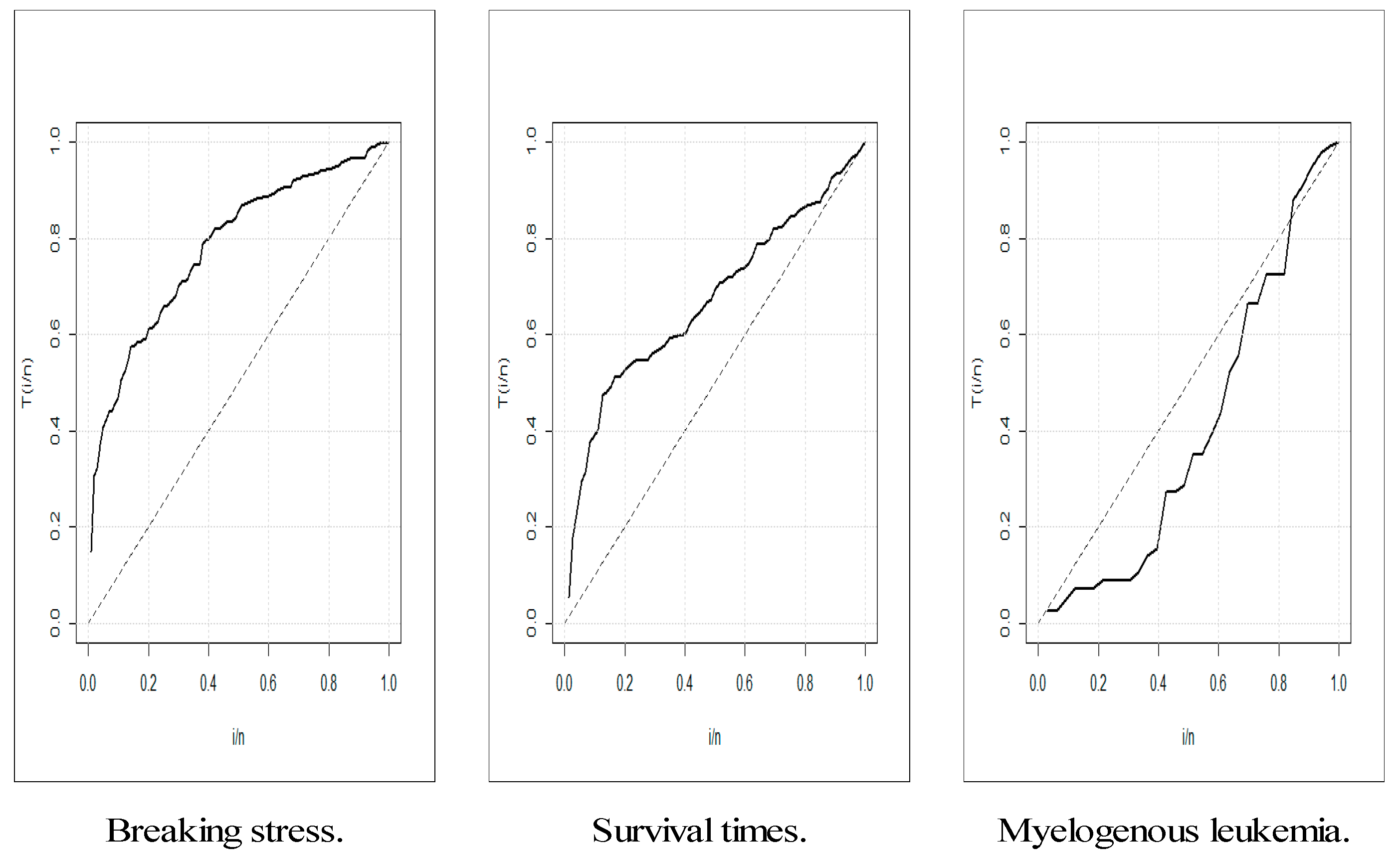
The 3rd data: {65, 156, 100, 134, 16, 108, 121, 4, 39, 143, 56, 26, 22, 1, 1, 5, 65, 56, 65, 17, 7, 16, 22, 3, 4, 2, 3, 8, 4, 3, 30, 4, 43} is called “leukemia data”. This real data set gives the survival times, in weeks, of 33 patients suffering from acute myelogenous leukemia. The total time test (TTT) plot (see [40]) is an important graphical approach to verify whether the data can be applied to a specific distribution or not. The TTT plots of the three real datasets are presented in Figure 2. This plot indicates that the empirical HRFs of the 1st and 2nd datasets are increasing. The empirical HRF is the bathtub for the 3rd dataset.

We consider the following goodness-of-fit statistics: The “Akaike information criterion” ($C_{\mathrm{AI}}$), “Bayesian information criterion” ($C_{\mathrm{Bayes}}$), “consistent Akaike information criterion” ($C_{\mathrm{CA}}$), and “Hannan-Quinn information criterion” ($C_{\mathrm{HQ}}$). Table A3, Table A4 and Table A5 (see the Appendix A) give the MLEs, standard errors (SEs), and confidence interval (CIs) for all datasets. The same tables give the statistics $C_{\mathrm{AI}}$, $C_{\mathrm{Bayes}}$, $C_{\mathrm{HQ}},$ and $C_{\mathrm{CA}}$ values for these datasets.

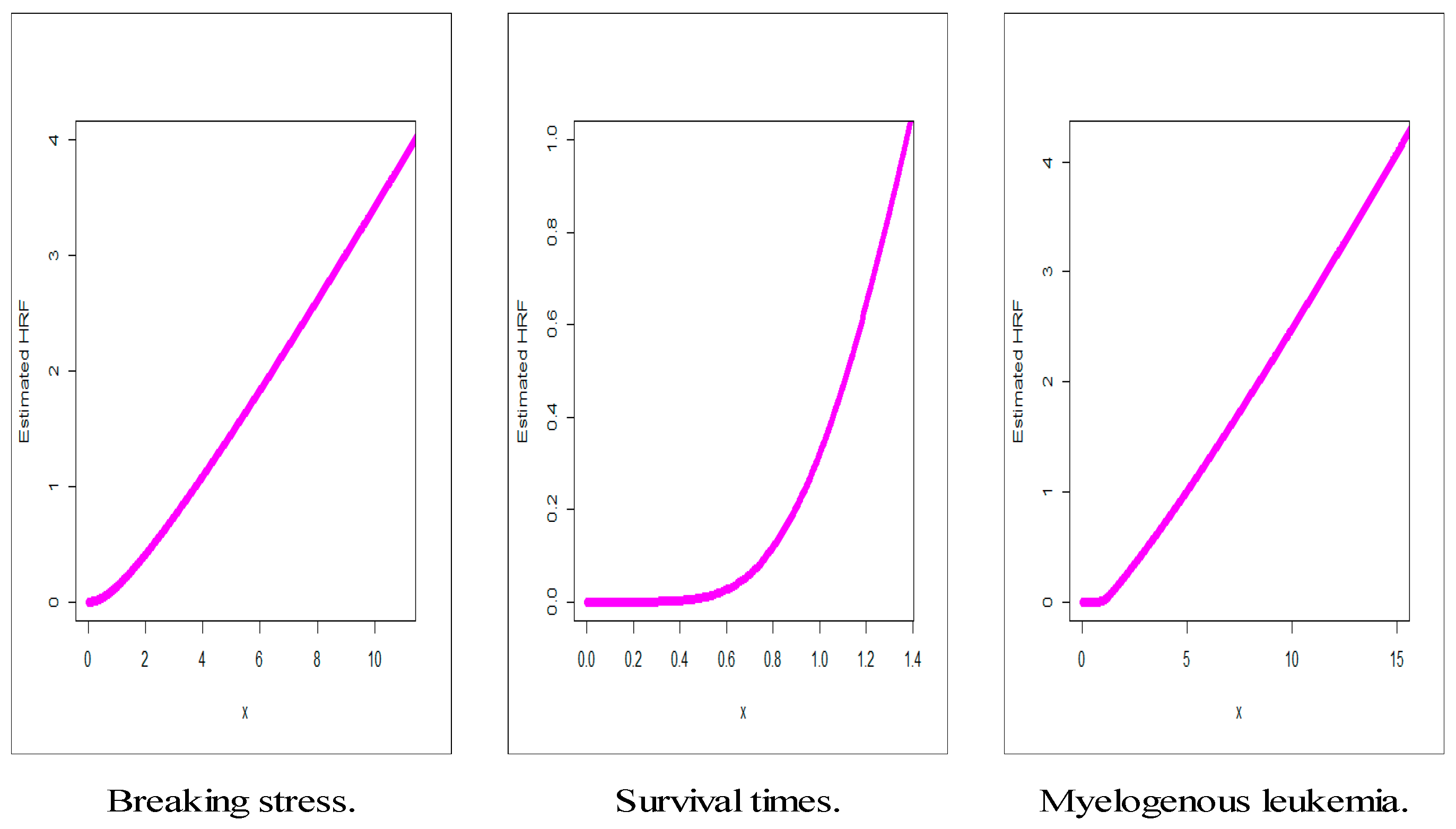
Based on the values in Table A3, we conclude that the RG-LL model provides the best fit as compared to other competitive models in the three applications with the smallest values of $C_{\mathrm{AI}}=302.75$, $C_{\mathrm{Bayes}}=301.17$, $C_{\mathrm{HQ}}=299.18,$ and $C_{\mathrm{CA}}=300.92$. Based on the values in Table A4, it is noted that the RG-LL model provides the best fit as compared to other competitive models in the three applications with the smallest values of $C_{\mathrm{AI}}=208.01$, $C_{\mathrm{Bayes}}=211.11$, $C_{\mathrm{HQ}}=207.12,$ and $C_{\mathrm{CA}}=209.53$. Based on the values in Table A5, it is noted that the RG-LL model provides the best fit as compared to other competitive models in the three applications with the smallest values of $C_{\mathrm{AI}}=313.44$, $C_{\mathrm{Bayes}}=316.41$, $C_{\mathrm{HQ}}=313.11,$ and $C_{\mathrm{CA}}=313.02$. Figure 2, Figure 3, Figure 4 and Figure 5 give the total time in test (TTT) plots, the estimated CDFs plots, the estimated PDFs plots, and the estimated HRFs plots, respectively. Based on Figure 2, the HRF of the three data are “monotonically increasing”, “monotonically increasing”, and “decreasing-constant-increasing”, respectively. Figure 3, Figure 4 and Figure 5 are provided for illustrating the superiority on the new model graphically.

Based on the values in Table A3, Table A4 and Table A5 and Figure 2, Figure 3, Figure 4 and Figure 5, we conclude that the RG-LL model provides good (and also the best) fits as compared to other competitive models in the three applications with smallest values of $C_{\mathrm{AI}}$, $C_{\mathrm{Bayes}}$, $C_{\mathrm{HQ}}$ and $C_{\mathrm{CA}}$.

5. The Modified BN-GOF Test

5.1. Censored Maximum Likelihood

Suppose that $Z_1,Z_2,\dots ..,Z_n$ is a RS with right censoring from the RG-LL$\left(\underset{\_}{\xi }\right)$ distribution. The observed data $z_i{|}_{\left(i=1,2,..,n\right)}=\stackrel{}{min}\left(Z_i,C_i\right)$ are the “minimum of the survival time” $Z_i$ and censoring time $C_i$ for each subject in the sample. Therefore, $z_i$ can be written as ${(z_i,{\nabla }_i)}_{i=1,2,\dots ,n}$ where ${\nabla }_i=1$ if $Z_i$ is the moment of failure (complete observation) and ${\nabla }_i=0$ if $Z_i$ is the “moment of censoring”. The likelihood function can be written as:

$$l\left(z,\underset{\_}{\xi }\right)={\Pi }_{i=1}^n{h}_{\theta ,a_1,a_2}{(z_i)}^{{\nabla }_i}{S}_{\theta ,a_1,a_2}\left(z_i\right){|}_{ \left({\nabla }_i=1_{Z_i<C_i}\right)}.$$

The log-likelihood function of RG-LL$\left(\underset{\_}{\xi }\right)$ distribution is:

$$L_{C_i}\left(\underset{\_}{\xi }\right)={\displaystyle \sum }_{i=1}^n{\nabla }_i\left[\begin{array}{c}\ln \left(\theta a_1{a}_2\right)+\left(a_2-1\right)\ln z_i\\ +\left(\theta -1\right)\ln {\varpi }_i+\ln ({\varpi }_i^2-1)\end{array}\right]-a_1{\displaystyle \sum }_{i=1}^n{\left({\varpi }_i^{\theta }-1\right)}^2,$$

where ${\varpi }_i=1+z_i^{a_2},$ and the score functions are obtained as follows:

$$\frac{\partial L_{C_i}\left(\underset{\_}{\xi }\right)}{\partial \theta }={\displaystyle \sum }_{i=1}^n{\nabla }_i\left[\frac{1}{\theta }+\ln \left({\varpi }_i\right)\right]-2a_1{\displaystyle \sum }_{i=1}^n{\varpi }_i^{\theta }\ln \left({\varpi }_i\right)\left({\varpi }_i^{\theta }-1\right),\frac{\partial L}{\partial a_1}={\displaystyle \sum }_{i=1}^n\frac{{\nabla }_i}{a_1}-{\displaystyle \sum }_{i=1}^n{\left({\varpi }_i^{\theta }-1\right)}^2,$$

and

$$\frac{\partial L_{C_i}\left(\underset{\_}{\xi }\right)}{\partial a_2}={\displaystyle \sum }_{i=1}^n{\nabla }_i\left[\frac{1}{a_2}+\ln z_i+\left(\theta -1\right)\frac{z_i^{a_2}\ln z_i}{{\varpi }_i}+\frac{2z_i^{a_2}\ln z_i{\varpi }_i}{{\varpi }_i^2-1}\right]-2a_1{a}_2\theta {\displaystyle \sum }_{i=1}^n{z}_i^{a_2} \ln z_i{\varpi }_i^{\theta -1}\left({\varpi }_i^{\theta }-1\right).$$

The $\mathrm{MLEs}$ of the unknown parameters can be obtained using various techniques, either software R, “EM algorithm”, or “Newton Raphson” method.

5.2. The Modified BN-GOF Test for Right Censored Data

Based on [23,24], the statistic test is defined as:

$$Y_n^2={\displaystyle \sum }_{j=1}^n\frac{1}{U_j}{\left(U_j-e_j\right)}^2+Q,$$

where $U_j$ and $e_j$ are the observed and the expected numbers of failure in grouping intervals, other elements were defined in [20,23,24]. The endpoints ${\rho }_j$ of $k$ random gouging intervals $I_j=\left[{\rho }_{j-1},{\rho }_j\right[$ are chosen so that the expected failure times to fall into these intervals are the same for each $j=1,..,k-1,$ ${\widehat{\rho }}_k=\max \left(z_{\left(l\right)},\tau \right).$ The estimated ${\widehat{\rho }}_j$ is defined by

$${\widehat{\rho }}_j=H^{-1}\left(\frac{E_j-{{\displaystyle \sum }}_{l=1}^{i-1}{H}_{\theta ,a_1,a_2}\left(z_l\right)}{n-i+1},\underset{\_}{\xi }\right),$$

and ${\widehat{\rho }}_k=\stackrel{}{max}\left(z_{\left(n\right),}\tau \right)$ where $H_{\theta ,a_1,a_2}\left(z_l\right)$ is the cumulative HRF (CHRF) of the model distribution. This statistic test $Y_n^2$ follows a chi-squared model.

5.3. Choice of Random Grouping Intervals

Suppose that $Z_1,Z_2,\dots ..,Z_n$ is a RS with right censoring from the RG-LL$\left(\underset{\_}{\xi }\right)$ model and a finite time $\tau$. The estimated ${\widehat{\rho }}_j$ is obtained as follows:

$${\widehat{\rho }}_j={\left[1-{\left(1+\sqrt{\frac{E_j-{{\displaystyle \sum }}_{l=1}^{i-1}{H}_{\theta ,a_1,a_2}\left(z_l\right)}{a_1\left(n-i+1\right)}}\right)}^{1/\theta }\right]}^{1/a_2}$$

where $H_{\theta ,a_1,a_2}\left(z_l\right)$ is the CHRF of the RG-LL $\left(\underset{\_}{\xi }\right)$ distribution.

5.4. Quadratic Form of $Q$ of the Statistic $Y_n^2$

To calculate the quadratic form $\mathit{Q}$ of the statistic $Y_n^2$, and as its distribution does not depend on the parameters, so we can use the estimated matrices $\widehat{\mathbf{W}}$, $\widehat{\mathbf{C}}$ and the estimated information matrix $\widehat{\mathbf{I}}$ The elements of $\widehat{\mathbf{C}}$ are defined in [20].

5.5. Estimated Information Matrix $\widehat{\mathit{I}}$

We need also the information matrix $\widehat{I}$ of the RG-LL $\left(\underset{\_}{\xi }\right)$ model with the right censoring. After difficult calculations and some simplifications, we have obtained the elements of the matrix as follows:

$${\widehat{ı}}_{11}=\frac{1}{n}{\displaystyle \sum }_{i=1}^n{\nabla }_i{\left[\frac{1}{\theta }+ln\left({\varpi }_i\right)\right]}^2,{\widehat{ı}}_{22}=\frac{1}{n}{\displaystyle \sum }_{i=1}^n\frac{{\nabla }_i}{a_1^2}$$

$${\widehat{ı}}_{33}=\frac{1}{n}{\displaystyle \sum }_{i=1}^n{\nabla }_i{\left(\frac{1}{a_2}+ln{z}_i+\left(\theta -1\right)\frac{z_i^{a_2}ln{z}_i}{{\varpi }_i}+\frac{2z_i^{a_2}ln{z}_i{\varpi }_i}{{\varpi }_i^2-1}\right)}^2, {\widehat{ı}}_{12}=\frac{1}{n}{\displaystyle \sum }_{i=1}^n\frac{{\nabla }_i}{a_1}\left[\frac{1}{\theta }+ln\left({\varpi }_i\right)\right]$$

$${\widehat{ı}}_{13}=\frac{1}{n}{\displaystyle \sum }_{i=1}^n{\nabla }_i\left[\frac{1}{\theta }+ln\left({\varpi }_i\right)\right]\left[\frac{1}{a_2}+ln{z}_i+\left(\theta -1\right)\frac{z_i^{a_2}ln{z}_i}{{\varpi }_i}+\frac{2z_i^{a_2}ln{z}_i{\varpi }_i}{{\varpi }_i^2-1}\right],$$

and

$${\widehat{ı}}_{23}=\frac{1}{n}{\displaystyle \sum }_{i=1}^n\frac{{\nabla }_i}{a_1}\left(\frac{1}{a_2}+ln{z}_i+\left(\theta -1\right)\frac{z_i^{a_2}ln{z}_i}{{\varpi }_i}+\frac{2z_i^{a_2}\ln z_i{\varpi }_i}{{\varpi }_i^2-1}\right).$$

Then, we obtain the statistic test for the RG-LL $\left(\underset{\_}{\xi }\right)$ distribution with the “right censored” data. This statistic follows a chi-squared distribution with $k$ degrees of freedom.

$$Y_n^2\left(\underset{\_}{\xi }\right) ={{\displaystyle \sum }}_{j=1}^r\frac{1}{U_j}{\left(U_j-e_j\right)}^2+{\widehat{W}}^T{\left[{\widehat{ı}}_{l{l}^{\prime }}-{{\displaystyle \sum }}_{j=1}^r{\widehat{C}}_{lj}{\widehat{C}}_{l^{\prime }j}{\widehat{A}}_j^{-1}\right]}^{-1}\widehat{W}.$$

6. Simulations under Censorship

In this section we perform a simulation study to consolidate our results. For this purpose, $N=\mathrm{10,000}$ censored samples (with sizes: $n=25, 50, 130, 350, 500, 1000)$ from the RG-LL$\left(\underset{\_}{\xi }\right)$ distribution is simulated.

6.1. Maximum Likelihood Estimation

We generate the simulated samples with various parameters. Using the R software and $BB$ algorithm, means simulated MLEs and their mean squared errors (MSEs) are calculated and given in

Table 1. The maximum likelihood estimators (MLEs) and their mean squared errors (MSEs).

N = 10,000	${\mathit{a}}_{\mathbf{1}}=\mathbf{0.5}$	${\mathit{a}}_{\mathbf{2}}=\mathbf{1.5}$	θ = 2
$n_1$= 25	0.5294(0.0096)	0.4621(0.0093)	1.9597(0.0086)
$n_2$= 50	0.5230(0.0089)	0.4731(0.0079)	1.9623(0.0067)
$n_3$= 130	0.5178(0.0072)	0.4774(0.0061)	1.9738(0.0052)
$n_4$= 350	0.5102(0.0058)	0.4822(0.0049)	1.9894(0.0038)
$n_5$= 500	0.5064(0.0046)	0.4876(0.0035)	1.9912(0.0024)
$n_6$= 1000	0.5012(0.0033)	0.4933(0.0023)	1.9985(0.0018)
	a₁ = 1.2	a₂ = 2.1	θ = 1.6
$n_1$= 25	1.7682(0.0074)	2.1296(0.0068)	1.5523(0.0113)
$n_2$= 50	1.1721(0.0053)	2.1233(0.0059)	1.5693(0.0096)
$n_3$= 130	1.1794(0.0042)	2.1188(0.0046)	1.5734(0.0084)
$n_4$= 350	1.1811(0.0031)	2.1113(0.0032)	1.5837(0.0073)
$n_5$= 500	1.1896(0.0021)	2.1095(0.0025)	1.5893(0.0058)
$n_6$= 1000	1.1989(0.0017)	2.1016(0.0019)	1.5974(0.0043)

. As shown in these results, the MLEs are convergent.

6.2. Test Statistic $Y^2$

For testing the null hypothesis $H_0$ that the “right censored” data become from the RG-LL model, we computed the criteria statistic $Y_n^2\left(\underset{\_}{\xi }\right)$ as defined above for $N=\mathrm{10,000}$ simulated samples from the hypothesized distribution with different sizes $\left(n=25, 50, 130, 350, 500, 1000\right)$. Then, we calculated empirical levels of significance, when $Y²>{\chi }_{\epsilon }^2\left(r\right)$, corresponding to theoretical levels of significance $\left(\epsilon =0.10, 0.05, 0.01\right)$, we choose $k=5$. The results are reported in

Table 2. Simulated levels of significance for $Y_n^2\left(\underset{\_}{\xi }\right)$ against the theoretical values.

N = 10,000	$\mathit{n}=\mathbf{25}$	$\mathit{n}=\mathbf{50}$	$\mathit{n}=\mathbf{130}$	$\mathit{n}=\mathbf{350}$	$\mathit{n}=\mathbf{500}$	$\mathit{n}=\mathbf{1000}$
ε = 1%	0.0042	0.0053	0.0076	0.0082	0.0091	0.0095
ε = 5%	0.0443	0.0459	0.0465	0.0473	0.0487	0.0496
ε = 10%	0.0941	0.0956	0.0962	0.0979	0.0986	0.0992

.

Based on Table 2, the test proposed in this work, can be used to fit data from this new model.

7. Censored Validation under Real Data

Example 1.

Reference [41] has reported survival data on 26 psychiatric inpatients admitted to the university of Iowa hospitals during the years 1935–1948. This sample is part of a larger study of psychiatric inpatients discussed by [42]. Data for each patient consists of age at rest admission to the hospital, sex, number of years of follow-up (years from admission to death or censoring), and patient status at the follow-up time. The data is given as:

1, 1, 2, 11, 14, 22, 22, 24, 25, 26, 28, 30*, 30*, 31*, 31*, 32, 33*, 33*, 34*, 35, 35*, 35*, 36*, 37*, 39*, 40. (*indicates the censorship). We use the statistic test provided above to verify if these data are modeled by RG-LL distribution, and at that end, we first calculate the MLEs of the unknown parameters

$$\underset{\_}{\xi }={\left({\widehat{a}}_1,{\widehat{a}}_2,\widehat{\theta }\right)}^T={\left(1.8391,2.538,3.748\right)}^T.$$

Data are grouped into $k=5$ intervals $I_j$. We give the necessary calculus in the

Table 3. Validation results.

${\widehat{\mathit{\rho }}}_{\mathit{j}}$		17.23	25.59	31.67	34.85	40
${\mathit{U}}_{\mathit{j}}$		5	4	6	4	7
${\widehat{\mathbf{C}}}_{lj}$	${\widehat{\mathbf{C}}}_{1j}$	2.0937	1.9374	1.239	1.0846	2.0934
	${\widehat{\mathbf{C}}}_{2j}$	2.7187	2.0646	1.0874	0.5437	1.0874
	${\widehat{\mathbf{C}}}_{2j}$	1.0236	0.8374	0.9138	0.8631	1.3193
$e_j$		4.6322	4.6322	4.6322	4.6322	4.6322

.

Then we obtain the value of the statistic test $Y_n^2$:

$$Y_n^2=X^2+Q=4.9325+3.0031=7.9356$$

For significance level = 0.05, the critical value ${\chi }_5^2$ = 11.0705 is superior than the value of $Y_n^2$ = 7.9356 (see

Table 4. $Y_n^2$ statistic to all competitive models.

Model	${\mathit{Y}}_{\mathit{n}}^{\mathbf{2}}$ Statistic
RG-LL	7.9356
MOBXII	8.5632
TLBXII	8.8319
KwBXII	8.3415
BEBXII	8.7196
BBXII	8.9317
FKwBXII	8.2413
WLL	9.4053
FBBXII	8.1232
BXII	8.4965

), so we can say that the proposed model RG-LL fits these data. We calculated also the test statistics $Y_n^2$ to fit these data to the competing models.

Example 2.

We consider the bone marrow transplant data (see [43]) for patients suffering from acute lymphoblastic leukemia. This data consists of time (in days) to death or on study time after an allogenic bone marrow transplant for 38 patients. The bone marrow transplant is a standard treatment for acute leukemia. Recovery following bone marrow transplantation is a complex process. Immediately following transplantation, patients have depressed platelet counts and have higher hazard rate for the development of infections but as the time passes the hazard decreases. Data are given as:

1, 86, 107, 110, 122, 156, 162, 172, 194, 226*, 243, 262, 262, 269, 276, 350*, 371, 417, 418, 466, 487, 526, 530*, 716, 781, 996*, 1111*, 1167*, 1182*, 1199*, 1279, 1330*, 1377*, 1433*, 1462, 1496*, 1602*, 2081*.

We use the statistic test provided above to verify if these data are modeled by the RG-LL distribution. Using the BB solve software, we calculate the maximum likelihood estimators of the unknown parameters:

$$\widehat{\xi }={\left({\widehat{a}}_1,{\widehat{a}}_2,\widehat{\theta }\right)}^T={\left(2.6138,4.9462,8.643\right)}^T.$$

Then, we grouped the observations into $r=5$ intervals $I_j$. The intermediate calculations are given in

Table 5. Values of ${\widehat{\rho }}_j$, $U_j$, $\stackrel{⌢}{C}$, and $e_j$ for the second data.

${\widehat{\mathit{\rho }}}_{\mathit{j}}$		171.865	325.593	510.362	1245.639	2081
${\mathit{U}}_{\mathit{j}}$		7	8	6	9	8
${\widehat{\mathbf{C}}}_{lj}$	${\widehat{\mathbf{C}}}_{1j}$	0.9356	0.8269	0.8139	0.6039	0.4964
	${\widehat{\mathbf{C}}}_{2j}$	1.4152	1.4153	1.0108	0.4043	0.2021
	${\widehat{C}}_{2j}$	1.2093	2.4136	1.5623	0.9462	0.8196
$e_j$		4.2385	4.2385	4.2385	4.2385	4.2385

.

The value of the statistic test $Y_n^2$ is obtained as follows:

$$Y_n^2=X^2+Q=4.9563+3.946=8.9023$$

Based on Table 5, the value of $Y_n^2=8.9023$ is less than the critical value ${\chi }_5^2=11.0705$–(for significance level $\epsilon =0.05),$ so we can say that these data can be fitted by the RG-LL model. Many useful uncensored real-life data sets in life testing, economies, medicine and engineering can be found in [44,45,46,47,48,49,50,51,52].

8. Conclusions

In this paper, a new three-parameter version of the log logistic model is introduced and studied. Some of its mathematical properties are derived. The new hazard rate function can be “asymmetric monotonically increasing”, “decreasing-constant”, “J shaped”, or “constant”. A simple type copula is considered for deriving many bivariate and multivariate extensions using “Farlie-Gumbel-Morgenstern Copula”, “modified Farlie-Gumbel-Morgenstern Copula”, “Clayton Copula”, and “Renyi’s entropy Copula”. Three applications to three real data sets are provided to illustrate the flexibility and importance of the new model. Using the approach of the “Bagdonavicius-Nikulin” goodness-of-fit test for right censored validation, we propose a new modified chi-square goodness-of-fit test for a new log-logistic model. The modified goodness-of-fit statistic test is applied for the right censored real dataset of survival times of psychiatric inpatients admitted to the university of Iowa hospitals. Based on the maximum likelihood estimators on initial data, the modified test recovers the loss in information while grouping data and follows chi-square distributions. All elements of the modified criteria tests are explicitly derived and given. Three real data applications are presented for measuring the flexibility and the importance of the new model under the uncensored scheme.

References

1. Farlie, D.J.G. The performance of some correlation coefficients for a general bivariate distribution. Biometrika 1960, 47, 307–323. [Google Scholar] [CrossRef]
2. Gumbel, E.J. Bivariate logistic distributions. J. Am. Stat. Assoc. 1961, 56, 335–349. [Google Scholar] [CrossRef]
3. Gumbel, E.J. Bivariate exponential distributions. J. Am. Stat. Assoc. 1960, 55, 698–707. [Google Scholar] [CrossRef]
4. Morgenstern, D. Einfache beispiele zweidimensionaler verteilungen. Mitteilingsblatt Fur Math. Stat. 1956, 8, 234–235. [Google Scholar]
5. Rodriguez-Lallena, J.A.; Ubeda-Flores, M. A new class of bivariate copulas. Stat. Probab. Lett. 2004, 66, 315–325. [Google Scholar] [CrossRef]
6. Pougaza, D.B.; Djafari, M.A. Maximum entropies copulas. In Proceedings of the 30th international workshop on Bayesian inference and maximum Entropy methods in Science and Engineering, Chamonix, France, 4–9 July 2011; pp. 329–336. [Google Scholar]
7. Balakrishnan, N.; Lai, C.D. Contin. bivariate Distrib; Springer Science & Business Media: Berlin/Heidelberg, Germany, 2009. [Google Scholar]
8. Nichols, M.D.; Padgett, W.J. A bootstrap control chart for Weibull percentiles. Qual. Reliab. Eng. Int. 2006, 22, 141–151. [Google Scholar] [CrossRef]
9. Bjerkedal, T. Acquisition of resistance in Guinea pigs infected with different doses of virulent tubercle bacilli. Am. J. Hyg. 1960, 72, 130–148. [Google Scholar] [PubMed]
10. Altun, E.; Yousof, H.M.; Hamedani, G.G. A new log-location regression model with influence diagnostics and residual analysis. Facta Univ. Ser. Math. Inf. 2018, 33, 417–449. [Google Scholar]
11. Altun, E.; Yousof, H.M.; Chakraborty, S.; Handique, L. Zografos-Balakrishnan Burr XII distribution: Regression modeling and applications. Int. J. Math. Stat. 2018, 19, 46–70. [Google Scholar]
12. Ibrahim, M. The compound Poisson Rayleigh Burr XII distribution: Properties and applications. J. Appl. Probab. Stat. 2020, 15, 73–97. [Google Scholar]
13. Ibrahim, M.; Yousof, H.M. A new generalized Lomax model: Statistical properties and applications. J. Data Sci. 2020, 18, 190–217. [Google Scholar]
14. Yadav, A.S.; Goual, H.; Alotaibi, R.M.; Ali, M.M.; Yousof, H.M. Validation of the Topp-Leone-Lomax model via a modified Nikulin-Rao-Robson goodness-of-fit test with different methods of estimation. Symmetry 2020, 12, 57. [Google Scholar] [CrossRef] [Green Version]
15. Yousof, H.M.; Majumder, M.; Jahanshahi, S.M.A.; Ali, M.M.; Hamedani, G.G. A new Weibull class of distributions: Theory, characterizations and applications. J. Stat. Res. Iran. 2018, 15, 45–82. [Google Scholar]
16. Yousof, H.M.; Altun, E.; Rasekhi, M.; Alizadeh, M.; Hamedani, G.G.; Ali, M.M. A new lifetime model with regression models, characterizations and applications. Commun. Stat.-Simul. Comput. 2019, 48, 264–286. [Google Scholar] [CrossRef]
17. Nasir, M.A.; Korkmaz, M.C.; Jamal, F.; Yousof, H.M. On a new Weibull Burr XII distribution for lifetime data. Sohag J. Math. 2018, 5, 47–56. [Google Scholar] [CrossRef]
18. Mansour, M.; Yousof, H.M.; Shehata, W.A.M.; Ibrahim, M. A new two parameter Burr XII distribution: Properties, copula, different estimation methods and modeling acute bone cancer data. J. Nonlinear Sci. Appl. 2020, 13, 223–238. [Google Scholar] [CrossRef] [Green Version]
19. Varadhan, R.; Gilbert, P. BB: An R package for solving a large system of nonlinear equations and for optimizing a high-dimensional nonlinear objective function. J. Stat. Softw. 2009, 32, 1–26. [Google Scholar] [CrossRef] [Green Version]
20. Goual, H.; Yousof, H.M. Validation of Burr XII inverse Rayleigh model via a modified chi-squared goodness-of-fit test. J. Appl. Stat. 2020, 47, 393–423. [Google Scholar] [CrossRef]
21. Goual, H.; Yousof, H.M.; Ali, M.M. Lomax inverse Weibull model: Properties, applications, and a modified Chi-squared goodness-of-fit test for validation. J. Nonlinear Sci. Appl. 2020, 13, 330–353. [Google Scholar] [CrossRef] [Green Version]
22. Goual, H.; Yousof, H.M.; Ali, M.M. Validation of the odd Lindley exponentiated exponential by a modified goodness of fit test with applications to censored and complete data. Pak. J. Stat. Oper. Res. 2019, 15, 745–771. [Google Scholar] [CrossRef]
23. Bagdonavičius, V.; Nikulin, M. Chi-squared goodness-of-fit test for right censored data. Int. J. Appl. Math. Stat. 2011, 24, 30–50. [Google Scholar]
24. Bagdonavičius, V.; Levuliene, R.J.; Nikulin, M. Chi-squared goodness-of-fit tests for parametric accelerated failure time models. Commun. Stat.-Theory Methods. 2013, 42, 2768–2785. [Google Scholar]
25. Burr, I.W. Cumulative frequency functions. Ann. Math. Stat. 1942, 13, 215–232. [Google Scholar] [CrossRef]
26. Burr, I.W. On a general system of distributions, III. The simple range. J. Am. Stat. Assoc. 1968, 63, 636–643. [Google Scholar]
27. Burr, I.W. Parameters for a general system of distributions to match a grid of α3 and α4. Commun. Stat. 1973, 2, 1–21. [Google Scholar] [CrossRef]
28. Burr, I.W.; Cislak, P.J. On a general system of distributions: I. Its curve-shaped characteristics; II. The sample median. J. Am. Stat. Assoc. 1968, 63, 627–635. [Google Scholar]
29. Rodriguez, R.N. A guide to the Burr type XII distributions. Biometrika 1977, 64, 129–134. [Google Scholar] [CrossRef]
30. Tadikamalla, P.R. A look at the Burr and related distributions. Int. Stat. Rev. 1977, 48, 337–344. [Google Scholar] [CrossRef]
31. Tadikamalla, P.R.; Johnson, N.L. Systems of frequency curves generated by transformations of logistic variables. Biometrika 1982, 69, 461–465. [Google Scholar] [CrossRef]
32. Yousof, H.M.; Ahsanullah, M.; Khalil, M.G. A new zero-truncated version of the Poisson Burr XII distribution: Characterizations and properties. J. Stat. Theory Appl. 2019, 18, 1–11. [Google Scholar] [CrossRef]
33. Korkmaz, M.C.; Yousof, H.M.; Rasekhi, M.; Hamedani, G.G. The Odd Lindley Burr XII Model: Bayesian Analysis, Classical Inference and Characterizations. J. Data Sci. 2018, 16, 327–353. [Google Scholar]
34. Mansour, M.; Rasekhi, M.; Ibrahim, M.; Aidi, K.; Yousof, H.M.; Elrazik, E.A. A New Parametric Life Distribution with Modified Bagdonavičius–Nikulin Goodness-of-Fit Test for Censored Validation, Properties, Applications, and Different Estimation Methods. Entropy 2020, 22, 592. [Google Scholar] [CrossRef]
35. Ibrahim, M.; Yousof, H.M. Transmuted Topp-Leone Weibull lifetime distribution: Statistical properties and different method of estimation. Pak. J. Stat. Oper. Res. 2020, 501–515. [Google Scholar] [CrossRef]
36. Ibrahim, M.; Mohammed, W.S.; Yousof, H.M. Bayesian and Classical Estimation for the One Parameter Double Lindley Model. Pak. J. Stat. Oper. Res. 2020, 16, 409–420. [Google Scholar]
37. Elsayed, H.A.H.; Yousof, H.M. The generalized odd generalized exponential Fréchet model: Univariate, bivariate and multivariate extensions with properties and applications to the univariate version. Pak. J. Stat. Oper. Res. 2020, 529–544. [Google Scholar] [CrossRef]
38. Al-Babtain, A.A.; Elbatal, I.; Yousof, H.M. A new three parameter Fréchet model with mathematical properties and applications. J. Taibah Univ. Sci. 2020, 14, 265–278. [Google Scholar]
39. Al-babtain, A.A.; Elbatal, I.; Yousof, H.M. A New Flexible Three-Parameter Model: Properties, Clayton Copula, and Modeling Real Data. Symmetry 2020, 12, 440. [Google Scholar] [CrossRef] [Green Version]
40. Aarset, M.V. How to identify a bathtub hazard rate. IEEE Trans. Reliab. 1987, 36, 106–108. [Google Scholar] [CrossRef]
41. Woolson, R.F. Rank Tests and a One-Sample Log Rank Test for Comparing Observed Survival Data to a Standard Population. Biometrika 1981, 37, 687–696. [Google Scholar] [CrossRef]
42. Tsuang, M.T.; Woolson, R.F. Mortality in Patients with Schizophrenia, Mania and Depression. Br. J. Psychiatry. 1977, 130, 162–166. [Google Scholar] [CrossRef]
43. Klein, J.P.; Moeschberger, M.L. Surviv. Anal: Tech. for Censored and Truncated Data; Springer Science & Business Media: Berlin/Heidelberg, Germany, 2003. [Google Scholar]
44. Aryal, G.R.; Yousof, H.M. The exponentiated generalized-G Poisson family of distributions. Econ. Qual. Control 2017, 32, 1–17. [Google Scholar] [CrossRef]
45. Hamedani, G.G.; Yousof, H.M.; Rasekhi, M.; Alizadeh, M.; Najibi, S.M. Type I general exponential class of distributions. Pak. J. Stat. Oper. Res. 2017, XIV, 39–55. [Google Scholar] [CrossRef] [Green Version]
46. Cordeiro, G.M.; Yousof, H.M.; Ramires, T.G.; Ortega, E.M.M. The Burr XII system of densities: Properties, regression model and applications. J. Stat. Comput. Simul. 2018, 88, 432–456. [Google Scholar] [CrossRef]
47. Korkmaz, M.C.; Yousof, H.M.; Hamedani, G.G.; Ali, M.M. The Marshall–Olkin generalized G Poisson family of distributions. Pak. J. Stat. 2018, 34, 251–267. [Google Scholar]
48. Hamedani, G.G.; Altun, E.; Korkmaz, M.C.; Yousof, H.M.; Butt, N.S. A new extended G family of continuous distributions with mathematical properties, characterizations and regression modeling. Pak. J. Stat. Oper. Res. 2018, 14, 737–758. [Google Scholar] [CrossRef] [Green Version]
49. Hamedani, G.G.; Rasekhi, M.; Najibi, S.M.; Yousof, H.M.; Alizadeh, M. Type II general exponential class of distributions. Pak. J. Stat. Oper. Res. 2019, XV, 503–523. [Google Scholar] [CrossRef]
50. Khalil, M.G.; Hamedani, G.G.; Yousof, H.M. The Burr X exponentiated Weibull model: Characterizations, mathematical properties and applications to failure and survival times data. Pak. J. Stat. Oper. Res. 2019, XV, 141–160. [Google Scholar] [CrossRef] [Green Version]
51. Korkmaz, M.C.; Altun, E.; Yousof, H.M.; Hamedani, G.G. The odd power Lindley generator of probability distributions: Properties, characterizations and regression modeling. Int. J. Stat. Probab. 2019, 8, 70–89. [Google Scholar] [CrossRef]
52. Nascimento, A.D.C.; Silva, K.F.; Cordeiro, G.M.; Alizadeh, M.; Yousof, H.M. The odd Nadarajah-Haghighi family of distributions: Properties and applications. Stud. Scientiarum Math. Hung. 2019, 56, 1–26. [Google Scholar] [CrossRef]
Figure 1. Plots of probability density function (PDF) and hazard rate function (HRF) for the Rayleigh generalized log-logistic (RG-LL) model.
Mathematics 08 01508 g001
Figure 2. Total time test (TTT) plots.
Mathematics 08 01508 g002
Figure 3. Estimated cumulative distribution functions (CDFs).
Mathematics 08 01508 g003
Figure 4. Estimated PDFs.
Mathematics 08 01508 g004
Figure 5. Estimated HRFs.
Mathematics 08 01508 g005