Abstract
To answer the question stated in the title, we present and compare two approaches: first, a standard approach for solving dual fuzzy nonlinear systems (DFN-systems) based on Newton’s method, which uses 2D FN representation and second, the new approach, based on multidimensional fuzzy arithmetic (MF-arithmetic). We use a numerical example to explain how the proposed MF-arithmetic solves the DFN-system. To analyze results from the standard and the new approaches, we introduce an imprecision measure. We discuss the reasons why imprecision varies between both methods. The imprecision of the standard approach results (roots) is significant, which means that many possible values are excluded.
1. Introduction
Solving linear and nonlinear fuzzy equations is a difficult task. This is evidenced by the fact that scientists are constantly developing new and better methods, because previous methods are not satisfactory and scientists have recognized the need to improve them. In the case of fuzzy nonlinear equations, one of the first methods was published in 1990 [1].
Newton’s numerical methods for solving DFN-systems are widespread in the literature. Abbasbandy and Asady proposed the numerical parametric approach to find a fuzzy nonlinear equation using Newton’s method. The efficiency of the algorithm was shown based on some numerical examples [2]. The continuation of their work is found in [3]. Ramli et al. show that the disadvantages of Newton’s method arise from the need to calculate and invert the Jacobian matrix at each iteration. They proposed an eight-step algorithm to solve fuzzy nonlinear equations [4]. In [5], Kajani et al. have applied Newton’s method for solving a DFN-system, which cannot be replaced by a fuzzy nonlinear system according to fuzzy arithmetic. Newton’s method was also used to solve dual fuzzy polynomial equations, where the modified Adomian decomposition method was applied in the numerical algorithm [6]. Waziri and Majid proposed a new approach for solving DFN-equations by combining Newton’s method for initial iteration and Broyden’s method for the rest of the iterations [7]. The paper [8] presents a method of solving DFN-systems based on Chord Newton’s method as an improvement of Newton’s iterative method published in [5]. An unquestionable advantage of the method [8] is that it requires the Jacobian matrix to be calculated only once for all iterations whereas in Newton’s method from [5] the matrix has to be calculated in each subsequent iteration, which is connected with a high computational effort. Wang et al. introduced the general family of n-point Newton-type iterative methods for solving nonlinear equations using direct Hermite interpolation [9]. All these approaches have one thing in common, as will be shown, which is they give imprecise results.
In the paper, we compare two approaches to solve DFN-systems first, a standard based on Newton’s method and a 2D FN representation. The second is a novel alternative approach based on multidimensional fuzzy arithmetic. We introduce imprecision to measure how different a solution is from the universal algebraic solution to analyze both methods’ solutions. The universal algebraic solution is a set of all solutions that satisfied the equations. We show that the standard approach finds a narrower set of solutions than the universal algebraic solution, which means that they omit many possible values. Our proposal’s primary motivation is the advantage of determining all possible results when looking for solutions, not only the most narrow subset. The full universal algebraic solution is especially desired in decision support systems, where the imprecision of traditional approaches leads to limitations of possible states and, therefore, may constitute decision variants.
The paper is organized as follows: first, we give some essential basic definitions in a standard approach and proposed MF-arithmetic in Section 2. The ideas for both approaches are compared in Section 3. The imprecision measure is defined in Section 4. In Section 5, we solve the benchmark DFN-system using both proposed approaches. Finally, in Section 6, we discuss the most important outcomes.
2. Preliminaries
Definition 1.
[5] The dual fuzzy nonlinear system [8] is understood to be the system (1):
where all parameters are fuzzy numbers.
The standard approach to solving DFN-systems applies Newton’s algorithm and a parametric form of a fuzzy number. Our approach uses MF-arithmetic based on a horizontal fuzzy number definition.
2.1. Basic Definitions in the Standard Approach
The definitions presented in the subsection are fundamental standard approaches using Newton’s methods for solving DFN-systems and comes from articles: [5,8].
Definition 2.
A fuzzy number is a fuzzy set like which satisfies:
- 1.
- u is upper semicontinuous,
- 2.
- outside some interval ,
- 3.
- There are real numbers such that and
- (a)
- is monotonic increasing on
- (b)
- is monotonic decreasing on
- (c)
Definition 3.
A fuzzy number in parametric form is a pair of functions , which satisfies the following:
- 1.
- is a bounded monotonic increasing left continuous function,
- 2.
- is a bounded monotonic decreasing left continuous function,
- 3.
- , .
where the variable r represents the membership level.
A popular triangular fuzzy number with the parameters (shown in Figure 1 (left graph)) in its parametric form is:
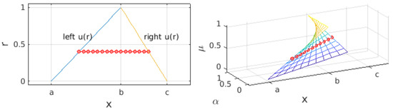
Figure 1.
Triangle membership function of a fuzzy number X with the cut at membership level : left graph—parametric fuzzy number (FN), right graph—horizontal FN.
In [8] the described Chord–Newton’s approach was implemented according to the following steps:
- Step 1
- Transform the dual fuzzy nonlinear equations into parametric form.
- Step 2
- Determine the initial point by solving the parametric equations for and .
- Step 3
- Compute the Jacobian matrix
- Step 4
- Compute (3)
- Step 5
- Repeat steps from 3 to 4 and continue with the next n keeping Jacobian until tolerance is satisfied.
2.2. Multidimensional Fuzzy Arithmetic
The MF-arithmetic theoretical foundations are linked with the horizontal fuzzy numbers (HFN) [10]. The HFN with linear or/and nonlinear left and right borders can be defined based on the FN parametric definition.
Definition 4.
A horizontal fuzzy number, of an arbitrary fuzzy number is defined as follows:
where and μ represents the membership level.
The variable is the Relative Distance Measure (RDM) [11,12] and ensures obtaining any FN value between the left border and right border . For value of the left endpoint and for the right endpoint of FN.
The fuzzy number U represents only an approximate knowledge about the precise but unknown true value of the variable (epistemic approach [13]).
If we have an approximate knowledge of two uncertain values of the variables x and y in the form of horizontal membership function: and then the basic arithmetic operations can be expressed as Equation (5).
The division operation guarantees a result in the form of a single granule if the following condition is satisfied: . However, if then the quotient will be multi-granular [14]. It should be noted that the result of any arithmetic operation is not defined in 2D space but in 4D space .
Definition 5.
[10] The direct solution of an operation on n horizontal fuzzy numbers , where is a set of numbers expressed in the form of multidimensional formula with up to n HFN variables .
Definition 6.
[10] For the direct solution of the basic arithmetic operations on n horizontal fuzzy numbers span is a fuzzy number:
Multidimensional fuzzy arithmetic has such important mathematical properties as (assuming are HFN):
- Additive inverse element ,
- Multiplicative inverse element ,
- Distributive law ,
- Cancellation law for multiplication , and others.
These properties allow solving any problem by transforming fuzzy equations from one mathematical form to another. In other words, without these properties, transformations are impossible. 2D-fuzzy arithmetic methods do not have such properties, which causes calculation difficulties.
3. Multidimensional Fuzzy Arithmetic Approach
What we called a standard approach are two-dimensional (2D) versions of the fuzzy arithmetic, and calculus based on it is presented in the scheme in Figure 2.
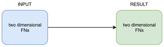
Figure 2.
A standard approach (2D) scheme in fuzzy arithmetic.
This approach assumes that the result of calculations on 2D-FNs is also a 2D-FN. Reference [12] considers this assumption incorrect. Such the approach delivers: sometimes precise, sometimes imprecise, sometimes paradoxical results or sometimes they are not able to solve the problem at all [15] or sometimes they can only solve it partially, as in the case of the benchmark (Equation (9)).
On the other hand, multidimensional fuzzy arithmetic works according to a different scheme than standard fuzzy 2D arithmetics. The diagram is given in Figure 3.
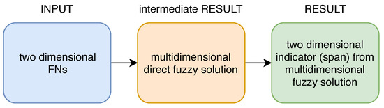
Figure 3.
A proposed multidimensional fuzzy (MF)-arithmetic approach scheme.
In 2D fuzzy calculation methods, what is assumed to be a “result” in MF-arithmetic is only a 2D indicator of a multidimensional result, which at most can be called “secondary result”. There are three basic indicators for the multidimensional fuzzy result:
- Span,
- Cardinality distribution,
- Center of gravity.
What is interpreted as the “result” in 2D methods is actually only the span of the multidimensional fuzzy result [16,17]. Until now, MF-arithmetic has been described in about 40 papers [15].
4. Imprecision Measure
Before numerical example presentation and further discussion, let us define a DFN-systems solution quality measure named “imprecision”. This quality is related to the concept of a universal algebraic solution. Let:
- -solution—universal algebraic solution always satisfies the given nonlinear equation regardless of its mathematical form (right and left sides of the equation are equal),
- A—-solution delivered by the method in the form of an MF-arithmetic,
- B—a solution delivered by the method in the form of a fuzzy number (FN),
- —the support of B FN,
- —the support of the A’s span .
Definition 7.
The imprecision of a solution B is a measure of how different a solution B is from the A which is -solution:
The imprecision calculates the percentage of values excluded (negative Imprecision for the case ) or values included (positive Imprecision for the case ) from or to the -solution.
5. Solving the Benchmark Equation
The best proof of methods qualitative correctness and precision is the correct solution to real problems. To show the performance of Newton’s approach, authors in [7] present solutions to some DFN-systems benchmark problems. To compare the standard and proposed MF-arithmetic approaches we take the benchmark from [5,7] called Problem 1.
Problem 1
([8]). Consider the dual fuzzy nonlinear equation:
In this problem denotes triangle FN with a core and with a left and right deviation equal to 2 and denotes a FN with a core equal to and both deviations equal to 1. The above FNs are shown in Figure 4.
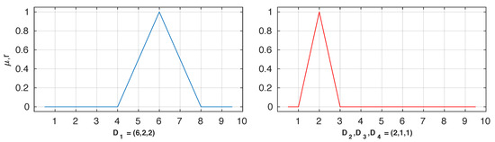
Figure 4.
Triangle fuzzy numbers , , , used as uncertain coefficients in the discussed benchmark Problem 1.
5.1. Standard Approach
Using the standard approach using Newton’s method and parametric FN representation, the authors of [5,8] achieved only one positive solution (positive root) of Equation (9) in form of the fuzzy number shown in Figure 5.
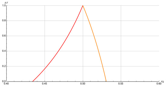
Figure 5.
Solution of the benchmark Equation (9) achieved with the use of a standard approach based on Newton’s methods presented in [5,8].
As will be shown, the positive solution delivered by the standard approach is, to a considerable degree, imprecise due to the FN definition and followed by its assumptions. Additionally, according to the authors [5,8] the negative solution of the benchmark Equation (9) does not exist at all and the explanation for this fact is given in [5].
5.2. MF-Arithmetic Approach
The benchmark equation (Equation (9)) represents a stationary, real system (Equation (10)),
where are true, crisp coefficients describing properties in the real system. In the analysed benchmark these true values are not known exactly. However, we have approximate knowledge about them: , , , . The fact that
does not imply that the true coefficient values are equal, i.e., . The probability of such a case occurring is equal to zero, because it is the probability of drawing a single point from a cuboid (geometric probability).
In terms of multidimensional fuzzy arithmetic the mathematical models of true and possible coefficient values are described as follows (Equation (14)):
To achieve benchmark (Equation (9)) solutions, the expression obtained in (Equation (14)) is substituted in equations (Equation (13)):
The and possible values satisfy the following conditions: and and their denominators do not include zero. Hence, the solutions are single information granules. Each information granule is multidimensional (6D) because and .
They are universal, algebraic solutionsof the benchmark, that can be easily verified by substitution in the Equation (9). The solutions ensure left and right-hand side equality regardless of the mathematical representation of the benchmark equation, which means that they are universal [11,12,15]. The multidimensional, algebraic solutions and are hypersurface fragments in 6D spaces and cannot be visualised. For simplified (2D) information about the solutions, low-dimensional indicators can be used such as: span, cardinality distribution and center of gravity of multidimensional fuzzy solution [11,12,15,17]. Spans of multidimensional solutions can be obtained with Equation (16).
To determine the span of the negative root (Equation (17)) equation, Equation (15) is substituted to Equation (16).
According to the authors of [8] the negative root does not exist. The lack of the negative solution is the consequence of the parametric FN form and the low-dimension fuzzy calculus. Newton’s methods [5,8] found the second root that does not satisfy the third condition in Definition 3 and therefore was rejected. We observe that the low-dimensional fuzzy calculus is imprecise. It is strange that the negative root was rejected, because negative crisp benchmark solutions can easily be found. The span function of the negative root , which is the benchmark (Equation (9)) solution, is shown in Figure 6.
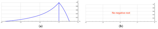
Figure 6.
The span function of the negative multidimensional solution (root) of the benchmark (9) determined using MF-arithmetic (a) and solution found with a standard approach based on Newton’s method [5,8] (b). (a) MF-arithmetic approach; (b) standard approach based on Newton’s method.
The minimum value of the negative root,
was obtained for following values of RDM-variables:
and the membership level and is equal to
The maximum value of the negative root,
was derived for the set of RDM-variables:
and the level and is equal to
These results can easily be verified with a method described in [17]. Solving equations (Equation (14)) by substituting RDM-variables for and results in a set of corresponding coefficient values:
All these values are possible because they are contained in supports of fuzzy coefficients in the benchmark (Equation (9)). For these coefficients the equation (Equation (9)) takes form:
and have two roots: and . The negative root is the same as that found using multidimensional fuzzy arithmetic.
Now we check the correctness of the solution. Coefficient values corresponding to RDM-variables and are
They generate a possible form of the Equation (9):
which has a negative root and also a positive .
Other combinations of RDM-variables
generate intermediate values of the negative root as shown in Figure 6, which can be easily checked.
The above is an empirical proof that the negative solution (root) of the benchmark (Equation (9)) exists.
The positive solution (root) of the benchmark (Equation (9)) can be determined on the basis of Equations (15) and (16) and its span function is as follows:
The minimum, left border of this function is evaluated for the RDM-variable set and the maximum, right border corresponds to the set: . Span functions determined by multidimensional fuzzy arithmetic and the standard approach are shown in Figure 7.
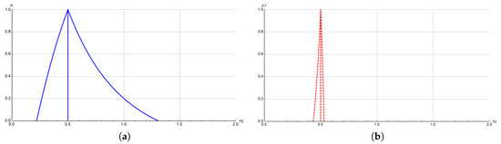
Figure 7.
The span function of the positive root determined by MF-arithmetic (a) and with standard approach using Newton’s method [5,8] (b). (a) MF-arithmetic approach; (b) standard approach.
The result in Figure 7b delivered by Newton’s method seems to be of better quality (less uncertain), as its support is narrower than the support of the span function calculated using multidimensional fuzzy arithmetic (Figure 7a). If we expect the correct result to be precise and true, such a conclusion would be considered incorrect. The correct result does not necessarily mean less uncertain (narrower).
Let us check whether the standard approach result is possible and true. According to [8] possible solutions (only the positive root) for the benchmark (9) on the membership level are in the range As a consequence every lying outside of the interval is not possible. The validity of this conclusion can be easily verified by the following reasoning. The values of RDM-variables and correspond to coefficients:
which generate the possible benchmark (9) form:
Such quadratic equation has two roots and the positive root is It means that such root value is possible. However, according to the standard approach using Newton’s method, this value is impossible.
Moreover, RDM-variable values and resulted in
coefficients that transforms the benchmark Equation (9) into the form
This quadratic equation has a positive root , which according to the standard approach (Figure 7b), is impossible. Other intermediate, possible values of the root can be achieved for other combinations of RDM-variables
5.3. Final Comparison
The total comparison of all solutions (roots) obtained with multidimensional fuzzy arithmetic and with the standard approach using Newton’s method and parametric FN representation is shown in Figure 8.
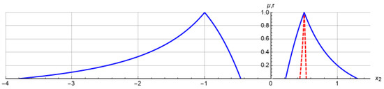
Figure 8.
All solutions (roots) calculated with multidimensional fuzzy arithmetic (continuous line) and with the standard approach using Newton’s method (dashed line).
We claim that the results of the standard approach are, to some degree, imprecise. Let us calculate the imprecision based on Definition 7. The standard Newton method excludes over 91% possible positive root solutions compared to possible solutions delivered by multidimensional fuzzy arithmetic:
The number of solutions excluded from the negative root is 100%.
The experimental verification shows that roots: and computed by MF-arithmetic are true and possible. On this basis, we can conclude that the standard Newton method solution is significantly imprecise.
6. Conclusions
Using an example and solving the DFN-equation benchmark, we compare the standard approach based on Newton’s method, which uses 2D FN representation to the MF-arithmetic approach. Calculating the imprecision measure, we show that the standard approach results are significantly imprecise, i.e., differs from the universal algebraic solution (UA-solution). According to the standard approach, the benchmark equation’s negative root does not exist at all, and the positive root is significantly (over 91%) imprecise (underestimated). The reason for such imprecision is twofold. First is the fuzzy numbers representation and, consequently, the low-dimensional fuzzy calculus, i.e., striving for a direct calculation of results without prior determination of the multidimensional, universal, algebraic fuzzy result. Second, the assumptions in the fuzzy number representation reject the negative root.
The precise solution of DFN-systems can be achieved with the MF-arithmetic, which works according to the scheme:
- Get 2D fuzzy inputs,
- Calculate a multidimensional direct fuzzy result,
- Calculate the 2D secondary result.
Based on the presented example, we stated that without the multidimensional fuzzy calculation, in general, true and precise solutions for DFN-systems are impossible to obtain. The standard approach has limited applications for solving dual fuzzy nonlinear systems due to a high imprecision, i.e., by rejecting a range of possible values.
In future work, we explore MF-arithmetic applicability for solving other types of equations and systems of equations. We plan to apply our approach to real decision-making problems.
Author Contributions
Conceptualization, A.P. and J.K.; methodology, A.P., J.K.; software, J.K.; validation, A.P., J.K. and W.S.; formal analysis, A.P. and J.K.; investigation, J.K.; resources, J.L. and W.S.; data curation, J.K.; writing—original draft preparation, J.K., A.P. and W.S.; writing—review and editing, J.K. and W.S.; visualization, J.K.; supervision, A.P. and W.S.; project administration, J.K.; funding acquisition, W.S. All authors have read and agreed to the published version of the manuscript.
Funding
The work was supported by statutory funds of the Research Team on Intelligent Decision Support Systems, Department of Artificial Intelligence and Applied Mathematics, Faculty of Computer Science and Information Technology, West Pomeranian University of Technology in Szczecin.
Acknowledgments
The authors would like to thank the editor and the anonymous reviewers, whose insightful comments and constructive suggestions helped us to significantly improve the quality of this paper.
Conflicts of Interest
The authors declare no conflict of interest.
Abbreviations
The following abbreviations are used in this manuscript:
| DFN-system | Dual Fuzzy Nonlinear System |
| FN | Fuzzy Number |
| RDM | Relative Distance Measure |
| MF-arithmetic | Multidimensional Fuzzy Arithmetic |
References
- Buckley, J.J.; Qu, Y. Solving Linear and Quadratic Fuzzy Equations. Fuzzy Sets Syst. 1990, 38, 43–59. [Google Scholar] [CrossRef]
- Abbasbandy, S.; Asady, B. Newton’s Method for Solving Fuzzy Nonlinear Equations. Appl. Math. Comput. 2004, 159, 349–356. [Google Scholar] [CrossRef]
- Abbasbandy, S.; Ezzati, R. Newton’s method for solving a system of fuzzy nonlinear equations. Appl. Math. Comput. 2006, 175, 1189–1199. [Google Scholar] [CrossRef]
- Ramli, A.; Abdullah, M.L.; Mamat, M. Broyden’s method for solving fuzzy nonlinear equations. Adv. Fuzzy Syst. 2010, 2010, 763270. [Google Scholar] [CrossRef]
- Kajani, M.T.; Asady, B.; Vencheh, A.H. An Iterative Method for Solving Dual Fuzzy Nonlinear Equations. Appl. Math. Comput. 2005, 167, 316–323. [Google Scholar] [CrossRef]
- Mosleh, M. Solution of dual fuzzy polynomial equations by modified Adomian decomposition method. Fuzzy Inf. Eng. 2013, 5, 45–56. [Google Scholar] [CrossRef]
- Waziri, M.Y.; Majid, Z.A. A New Approach for Solving Dual Fuzzy Nonlinear Equations Using Broyden’s and Newton’s Methods. Adv. Fuzzy Syst. 2012, 2012, 682087. [Google Scholar] [CrossRef][Green Version]
- Waziri, M.Y.; Moyi, A.U. An Alternative Approach for Solving Dual Fuzzy Nonlinear Equations. Int. J. Fuzzy Syst. 2016, 18, 103–107. [Google Scholar] [CrossRef]
- Wang, X.; Qin, Y.; Qian, W.; Zhang, S.; Fan, X.A. Family of Newton Type Iterative Methods for Solving Nonlinear Equations. Algorithms 2015, 8, 786–798. [Google Scholar] [CrossRef]
- Landowski, M. Method with horizontal fuzzy numbers for solving real fuzzy linear systems. Soft Comput. 2019, 23, 3921–3933. [Google Scholar] [CrossRef]
- Piegat, A.; Landowski, M. Fuzzy Arithmetic Type 1 with Horizontal Membership Functions. In Uncertainty Modeling: Dedicated to Professor Boris Kovalerchuk on his Anniversary; Springer International Publishing: Cham, Switzerland, 2017; pp. 233–250. [Google Scholar]
- Piegat, A.; Landowski, M. Is Fuzzy Number the Right Result of Arithmetic Operations on Fuzzy Numbers? In Advances in Fuzzy Logic and Technology 2017; Kacprzyk, J., Szmidt, E., Zadrożny, S., Atanassov, K.T., Krawczak, M., Eds.; Springer International Publishing: Cham, Switzerland, 2018; pp. 181–194. [Google Scholar]
- Lodwick, W.A.; Dubois, D. Interval Linear Systems As a Necessary Step in Fuzzy Linear Systems. Fuzzy Sets Syst. 2015, 281, 227–251. [Google Scholar] [CrossRef]
- Piegat, A.; Pluciński, M. Fuzzy number division and the multi-granularity phenomenon. Bull. Pol. Acad. Sci. Tech. Sci. 2017, 65, 497–511. [Google Scholar] [CrossRef]
- Piegat, A.; Landowski, M. Why Multidimensional Fuzzy Arithmetic? In Proceedings of the 13th International Conference on Theory and Application of Fuzzy Systems and Soft Computing—ICAFS-2018; Istanbul, Turkey, 28–30 October 2018, Aliev, R.A., Kacprzyk, J., Pedrycz, W., Jamshidi, M., Sadikoglu, F.M., Eds.; Springer International Publishing: Cham, Switzerland, 2019; pp. 16–23. [Google Scholar]
- Piegat, A.; Landowski, M. Two Interpretations of Multidimensional RDM Interval Arithmetic-Multiplication and Division. Int. J. Fuzzy Syst. 2013, 15, 488–496. [Google Scholar]
- Piegat, A.; Landowski, M. Correctness-checking of uncertain-equation solutions on example of the interval-modal method. In Modern Approach in Fuzzy Sets, Intuitionistic Fuzzy Sets, Generalized Nets and Related Topics; IBS PAN: Warswa, Poland, 2014; pp. 159–170. [Google Scholar]
© 2020 by the authors. Licensee MDPI, Basel, Switzerland. This article is an open access article distributed under the terms and conditions of the Creative Commons Attribution (CC BY) license (http://creativecommons.org/licenses/by/4.0/).