The Non-Smooth and Bi-Objective Team Orienteering Problem with Soft Constraints

Abstract

In the classical team orienteering problem (TOP), a fixed fleet of vehicles is employed, each of them with a limited driving range. The manager has to decide about the subset of customers to visit, as well as the visiting order (routes). Each customer offers a different reward, which is gathered the first time that it is visited. The goal is then to maximize the total reward collected without exceeding the driving range constraint. This paper analyzes a more realistic version of the TOP in which the driving range limitation is considered as a soft constraint: every time that this range is exceeded, a penalty cost is triggered. This cost is modeled as a piece-wise function, which depends on factors such as the distance of the vehicle to the destination depot. As a result, the traditional reward-maximization objective becomes a non-smooth function. In addition, a second objective, regarding the design of balanced routing plans, is considered as well. A mathematical model for this non-smooth and bi-objective TOP is provided, and a biased-randomized algorithm is proposed as a solving approach.

1. Introduction

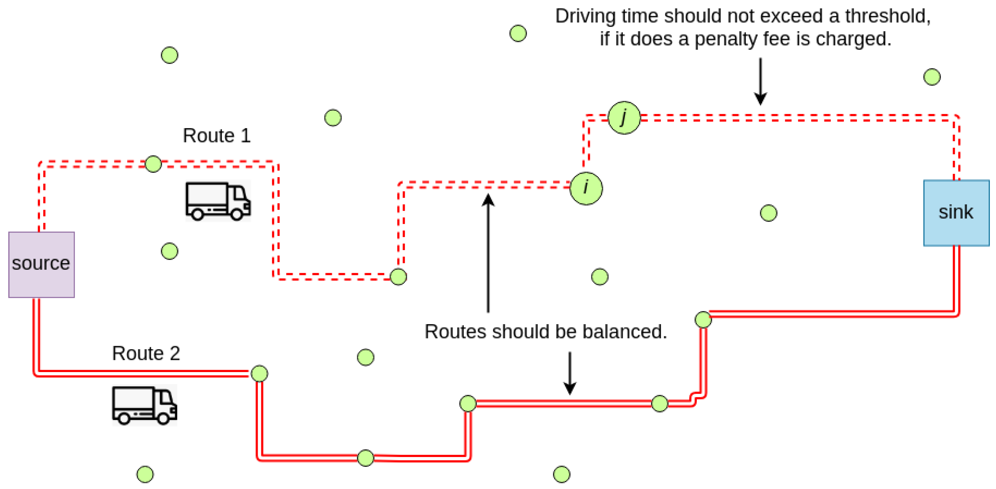
In the classical team orienteering problem (TOP), a fixed fleet of vehicles have to service a selection of customers, each of them offering a different reward [1]. A driving range constraint per route has to be strictly respected (hard constraint), and the goal is then to maximize the total reward collected. Hence, the manager has to select the nodes to be serviced as well as the order in which these nodes are visited. In this paper, we analyze a more realistic version of the TOP in which the hard constraint is substituted by a soft one, i.e., whenever the driving range limitation is violated, a piece-wise penalty cost is triggered, which might imply dealing with a non-smooth objective function. This variant is motivated by a recent experience related to the use of the TOP for modeling hospital logistics during the pandemic generated by the COVID-19 virus. Everyday during the months of March, April, and May 2020, hundreds of volunteers in the province of Barcelona (Spain) were producing sanitary masks and other items using home 3D printers. A reduced number of volunteer drivers were responsible to pick up sanitary items from a selected set of particular houses, and then bring these items to consolidation centers, where they were tested for quality, packed, and shipped to the corresponding hospitals. Each house produced a specific number of items per day, and the added value (reward) that was provided by each item unit was evolving during the pandemics (as inventories of some items were increasing). In this context, assuming a hard constraint for the number of driving hours (e.g., 6 h per day) was not fully realistic: sometimes, it could pay-off for the drivers to do a little extra effort in driving times, if, in return, this could lead to a noticeable increase in the aggregated reward of the items that were eventually delivered to the hospitals. In addition, while supporting this logistics process, we were asked to keep the work distribution across drivers as balanced as possible (to avoid an unfair distribution of the work load), thus transforming the optimization problem into a multi-criteria one [2]. A noticeable characteristic of this experience is that the details of the TOP were varying almost every day: the set of customers with available items were different (hence their locations and the travel time matrices were varying each day), the reward per item unit were also dynamic, as inventories of some items were more urgently needed depending on the daily evolution of the pandemics, sometimes there were priority constraints (e.g., one node had to be visited before others), customers were provided to us in a pre-clusterized format (e.g., by postal code or drivers’ preferences), etc. For this reason, we needed a flexible solving approach, i.e.: a methodology that could be easily adapted to the different TOP variants that were emerging day after day. At the same time, our approach had to be ‘agile’, in the sense that effective and efficient results were expected in a few minutes of computation, including aspects, such as the generation of the travel times for the daily set of customers. Based on our previous experience on related vehicle-routing optimization problems [3], we decided to develop a metaheuristic algorithm to solve the problem.

Recent applications of the TOP include the routing of unmanned aerial vehicles, or self-driving vehicles, to perform surveillance tasks [4]. The problem can be described, as follows: (i) consider an origin node, a destination node, a set of potential customers to be visited; (ii) consider a set of m vehicles, initially located at the origin, with a limited driving range capacity; and, (iii) the first time a customer is visited, a reward score is obtained. Under these circumstances, a solution to the problem is a set of m routes, connecting the origin node with the destination node, with each of these routes visiting a series of customers. The main goal is to maximize the total reward that was collected by the aforementioned routes without exceeding the driving-range capacity of any vehicle. This driving-range constraint usually refers to a maximum distance or time threshold (in the latter case, it can also include the servicing time at each customer). Due to this constraint, and to the fact that a reward is collected just the first time a customer is visited, any customer will be visited only once or not visited at all. Because the TOP can be seen as an extension of the well-known vehicle routing problem, it is also an NP-hard problem [5]. Therefore, the efficiency of exact methods is limited as the size of the problem grows, and it becomes necessary to employ metaheuristics to solve large-sized TOP instances. To the best of our knowledge, this is the first work discussing a non-smooth version of the TOP. Figure 1 provides an illustrative example of the considered non-smooth TOP, which considers two objectives: reward maximization and route balancing.

Regarding the main contributions of this paper, these can be stated as follows: (i) it proposes a mathematical formulation for the non-smooth and bi-objective TOP; (ii) a flexible and agile biased-randomized algorithm, which allows to solve the previously defined TOP; and, (iii) a series of computational experiments that contribute to illustrate the main concepts related to the non-smooth and bi-objective TOP. The rest of this manuscript is structured as follows: Section 2 offers a literature review on non-smooth optimization as well as on the TOP. Section 3 describes, in more detail, the specific version studied in this paper. The biased-randomized algorithm designed for solving the non-smooth TOP is provided in Section 4. Section 5 contains several numerical experiments that contribute to illustrate our methodology. Lastly, the main conclusions of this work, together with some open research lines, are provided in Section 6.

2. Related Work

This section briefly reviews related work on non-smooth optimization as well as on the team orienteering problem.

2.1. Non-Smooth Optimization

‘Smooth’ objective functions and constraints are frequently assumed in the optimization literature. When a function is smooth, it is a differentiable function with derivatives of all orders. Non-smooth optimization problems contain an objective function without the previous properties. From a combinatorial point of view, non-smooth optimization problems are similar to non-convex optimization problems: finding the optimal or near-optimal solution might require high computational effort. When no derivative information is available, determining the direction in which the function is increasing or decreasing becomes a challenging task. One has also to notice that the solution space might also have disjoint regions and, therefore, multiple local optima. In real-life applications, it is quite frequent to encounter non-convex and/or non-smooth objective functions. Thus, for example, Bagirov et al. [6] and by Karmitsa et al. [7] solve the minimum sum-of-squares clustering problem, which is formulated as a non-smooth and non-convex optimization problem. Incremental algorithms are employed as solving approaches. Actually, in the first paper a method based on the difference of convex functions is employed. In the second paper, the authors make use of the limited-memory bundle method. In order to test both solving methodologies and compare their efficiency, real-life data sets are used. These papers also utilize difference of convex functions to solve the non-parametric regression estimation problem. Their solving approach is based on the minimization of a non-convex and non-smooth empirical $L_2$-risk function.

Metaheuristic algorithms have been increasingly used to solve non-smooth and/or non-convex optimization problems in different application fields [8]. Thus, for instance, Al-Sultan [9] employ a tabu search algorithm to solve the clustering problem, while Oonsivilai et al. [10] use another tabu search algorithm to solve an optimization problem in the area of telecommunication networks. Similarly, Hemamalini and Simon [11] make use of an ant colony optimization approach for solving a non-smooth economic load dispatch problem. The same problem has been also addressed by Niknam et al. [12] and Basu [13], who propose the use of particle swarm optimization algorithms. In Schlüter et al. [14] and Corazza et al. [15], the authors make use of both ant colony optimization and particle swarm optimization to solve a non-smooth portfolio selection problem. Regarding the use of biased-randomized algorithms for solving non-smooth optimization problems, Juan et al. [16] introduced the MIRHA algorithm for solving the vehicle routing problem with soft constraints. Subsequently, Ferrer et al. [17] proposed a biased-randomized approach for solving a non-smooth version of the well-known permutation flow-shop problem. Likewise, De Armas et al. [18] used a biased-randomized algorithm to cope with the non-smooth arc routing problem, while Estrada-Moreno et al. [19] developed a similar approach for the non-smooth facility location problem. A recent review on the use of biased-randomized algorithms in non-smooth optimization problems is also available [20]. These algorithms have been also employed in other smooth optimization problems [21].

2.2. The Team Orienteering Problem

The orienteering problem was introduced by Golden et al. [22]. In its basic version, one vehicle has to select both the set of customers to service and the visiting order. Typically, not all customers can be visited due to the existence of a constraint that limits the maximum time or distance of the route. Because the orienteering problem is NP-hard, most of the solving approaches in the literature make use of metaheuristics. Gunawan et al. [23] provides an excellent overview of the many variations of the orienteering problem. Chao et al. [1] introduced the team orienteering problem, which extends the orienteering problem to the case in which several vehicles are considered. Once again, the goal is to maximize the total collected reward by selecting a subset of customers for each vehicle, as well as the visiting order. Additionally, a maximum time or distance per route is considered. The problem can be seen as a multi-level optimization one, where the following structure: (i) determine the set of customers to be visited; (ii) assign customers to the available vehicles in the fleet; and (iii) find the shortest path for each vehicle around the assigned customers. For small- and mid-sized instances of the TOP (up to 100 customers, approximately), it is usually possible to obtain the optimal solution [24]. Still, most authors propose the use of metaheuristic algorithms, such as the tabu search algorithms and the variable neighborhood search algorithm introduced by Archetti et al. [25]. Dang et al. [26] proposed a particle swarm optimization (PSO) algorithm. These algorithms simulate the collective behavior of wild animals [27]. Lin [28] introduced a multi-start simulated annealing (SA) algorithm. By integrating an SA step into a multi-start procedure, the algorithm reduces the chances of getting trapped into a local optimum. An iterative procedure is activated, starting from a randomly generated solution. In each iteration, a new solution is selected from the neighborhood of the current solution. As in most SA algorithms, from time to time a worse solution is accepted as the new current (or base) solution. While Ferreira et al. [29] propose a genetic algorithm for solving the TOP, Ke et al. [30] describe a Pareto mimic algorithm. The latter employs a mimic operator to generate a new solution. It also contains a swallow operator, which inserts an infeasible customer before repairing solution. Recently, Panadero et al. [31] have employed a simheuristic algorithm to cope with a stochastic variant of the TOP, while Bayliss et al. [4] have proposed a learnheuristic to solve a dynamic version of the same.

3. Modeling the Bi-Objective Non-Smooth TOP (BONSTOP)

The BONSTOP model introduced in this section is based on the formulation proposed by Mirzaei et al. [32], which we extend and adapt to the specific version considered in this paper. Consider an undirected and weighted graph $G:=(V,E)$, being $V:=\{1,2,\dots ,n\}$ the set of vertices or nodes, and $E:=\left\{\right\{i,j\}\in \mathcal{P}(V):i\ne j\}$ the set of edges, where $\mathcal{P}\left(V\right)$ is the set of all subsets of V or powerset. Additionally, every edge, $\{i,j\}\in E$ has a non-negative travel time $t_{ij}\ge 0$ associated with it. The travel time is assumed to satisfy the triangular inequality. In our context, a route is a path with initial node 1 and final node n. A route, r, is described by its edges, $r:=\{\{1,i_1\},\{i_1,i_2\},\dots ,\{i_{s-1},i_s\},\{i_s,n\}\}$. Nodes, $i_1,i_2,\dots ,i_s$, are named proper nodes. Let ${\mathcal{R}}_s$ be the set of all routes with s proper nodes. It is clear that the number of elements of ${\mathcal{R}}_s$, $|{\mathcal{R}}_s|$, equals the number of s-permutations without repetition of the $n-2$ elements in the set of proper nodes, $P_s^{n-2}$. Hence, as shown in Equation (1), and proved in Appendix A, we have:

$$|{\mathcal{R}}_s|=P_s^{n-2}={\displaystyle \frac{(n-2)!}{(n-2-s)!}}=(n-2)(n-3)\cdots (n-2-s+1).$$

(1)

We indicate, by $\mathcal{R}$, the set of all the routes on G. Notice that $\mathcal{R}={\bigcup }_{s=1}^{n-2}{\mathcal{R}}_s$ and $|\mathcal{R}|={\sum }_{s=1}^{n-2}|{\mathcal{R}}_s|=\lfloor e(n-2)!-1\rfloor$. A m-solution, $\mathcal{S}:=\{r^1,r^2,\dots ,r^m\}$, is a set of $m\ge 1$ routes $r^i$ with no proper nodes in common. Additionally, each node $i\in V\backslash \{1,n\}$ is associated with a profit $p_i>0$, while $p_1:=p_n:=0$. If the first route $r^1$ contains s proper nodes, then the number of nodes yet to be assigned to the remaining $m-1$ routes (vehicles) is $n-2-s$. The following inequality must be verified: $n-2-s\ge m-1$, i.e.: $n-m-1\ge s$. As a consequence, the total number of routes that can be used to obtain m-solutions is given by Equation (2):

$$\sum _{s=1}^{n-m-1}{P}_s^{n-2}=\lfloor e(n-2)!-1\rfloor -\sum _{s=n-m}^{n-2}{P}_s^{n-2}.$$

(2)

Therefore, the growth of the solution space is factorial with respect to the number of nodes. The first objective function, named benefit function, can be written as in Equation (3):

$$max\sum _{k=1}^m\sum _{i=2}^{n-1}{p}_i{y}_i^k,$$

(3)

where $y_i^k$ is a binary decision variable that takes the value 1 if the vertex $i\in V\backslash \{1,n\}$ belongs to route $r^k$ ($k=1,\dots ,m$), and 0 otherwise. A second objective function, named balance function, is introduced with the purpose of generating ‘balanced’ solutions (i.e., solutions with routes of similar characteristics). In particular, the second objective consist in minimizing the difference between the highest and the lowest reward obtained by any vehicle, as expressed in Equation (4):

$$min\left\{\underset{k\in M}{max}\left\{\sum _{i=2}^{n-1}{p}_i{y}_i^k\right\}-\underset{k\in M}{min}\left\{\sum _{i=2}^{n-1}{p}_i{y}_i^k\right\}\right\}.$$

(4)

Our version of the TOP consist in determining a m-solution with m vehicles (routes), with each of them completing the task on or before a predetermined time threshold, $T_{max}$. This constraint might cause some nodes not to be visited. The benefit function must be maximized, while the balance function needs to be minimized. No capacity constraints are considered for the vehicles. In order to describe the constraints, we define the binary decision variables $x_{ij}^k$ ($k=1,\cdots ,m$), which take the value 1 if edge $\{i,j\}\in E$ belongs to route $r^k$, and 0 otherwise. Feasible m-solutions must satisfy a series of constraints, as described next. The routes of a m-solution always start at node 1 and finish at node n:

$$\sum _{k=1}^m\sum _{j=2}^n{x}_{1j}^k=\sum _{k=1}^m\sum _{i=1}^{n-1}{x}_{in}^k=m.$$

(5)

Each node in V$\backslash \{1,n\}$ is, at most, a proper node of one route in a given m-solution:

$$\sum _{k=1}^m{y}_i^k\le 1,\mathrm{for}\mathrm{all}i\in V\backslash \{1,n\}.$$

(6)

In a m-solution, each proper node in a route belongs to exactly two edges in the route:

$$\sum _{\{i,h\}\in E}{x}_{ih}^k=2y_h^k,\mathrm{for}\mathrm{all}h\in V\backslash \{1,n\},k=1,\cdots ,m.$$

(7)

For each route, the time restriction is established:

$$T_k:=\sum _{\{i,h\}\in E}{x}_{ij}^k{t}_{ij}=\sum _{i=1}^{n-1}\sum _{j=i+1}^n{x}_{ij}^k{t}_{ij}\le T_{max},k=1,\cdots ,m.$$

(8)

Finally, sub-tours are prohibited:

$$\sum _{i,j\in U,i<j}{x}_{ij}^k\le |U|-1,\mathrm{for}\mathrm{all}\{U\subseteq V\backslash \{1,n\}:|U|\ge 2\},k=1,\cdots ,m.$$

(9)

3.1. Soft Constraints

In many real-life applications, the possibility of violating certain constraints can be considered. Generally, these ‘soft constraints’ imply the application of a penalty cost whenever a threshold is exceeded. In our case, we will allow the vehicle to exceed the time-threshold $T_{\max }$ if, after accounting for the associated penalty cost, the value of the objective function is still improved. Therefore, constraints (8) will be considered as soft ones. Accordingly, for a given route k, its basic cost $f_k:={\sum }_{i=2}^{n-1}{p}_i{y}_i^k$ is extended, as follows:

$$f_k^{*}:=\left\{\begin{array}{cc}{f}_k\hfill & \mathrm{if}{T}_k\le T_{\max }\hfill \\ {\displaystyle \frac{T_{\max }}{\left(T_k+K\right)}}{f}_k\hfill & \mathrm{otherwise},\hfill \end{array}\right.$$

(10)

where $K\ge 0$ is an experimental design parameter. In particular, considering the variability of $T_{\max }$ for each instance of the selected benchmark, the value of K is set as a percentage of $T_{\max }$ to illustrate different degrees of flexibility: high flexibility ($K=0\%$ of $T_{\max }$), medium flexibility ($K=10\%$ of $T_{\max }$), and low flexibility ($K=50\%$ of $T_{\max }$).

3.2. Considering a Weighted Combination of Objectives

In a multi-objective optimization the quality of a solution is determined by its ‘dominance’ in any of the dimensions (objectives) being considered. The non-dominated set of solutions define the Pareto frontier, which is usually difficult to determine. In the case the different objectives are measured in the same units (e.g., monetary value), one can also transform the multi-objective function into a single-objective one by considering a weighted combination of the different objectives. These weighted-sum methods tend to be simple, but they assume that an expert is able to define the proper weight values. Hence, we can consider all of the constraints (5)–(9) and the following weighted objective function, where $\alpha \in (0,1)$:

$$max\alpha \sum _{k=1}^m\sum _{i=2}^{n-1}{p}_i{y}_i^k+\left(1-\alpha \right)\left(\underset{k\in M}{min}\left\{\sum _{i=2}^{n-1}{p}_i{y}_i^k\right\}-\underset{k\in M}{max}\left\{\sum _{i=2}^{n-1}{p}_i{y}_i^k\right\}\right).$$

(11)

However, when constraints (8) are taken as soft ones, a penalty coefficient–given by (10)—is added to the first term of the weighted objective function:

$$max\alpha \sum _{k=1}^m{f}_k^{*}+\left(1-\alpha \right)\left(\underset{k\in M}{min}\left\{\sum _{i=2}^{n-1}{p}_i{y}_i^k\right\}-\underset{k\in M}{max}\left\{\sum _{i=2}^{n-1}{p}_i{y}_i^k\right\}\right).$$

(12)

Therefore, in this second case, it is actually possible to violate constraints (8) by incurring in a well-defined penalty cost. Notice that it is possible to consider a non-smooth version of the model with continuous variables by substituting the binary ones $y_i^k,x_{ij}^k\in \{0,1\}$ by the constraints $y_i^k(1-y_i^k)=0$, $x_{ij}^k(1-x_{ij}^k)=0$, and $y_i^k$, $x_{ij}^k\in [0,1]$.

4. A Biased-Randomized Algorithm for the BONSTOP

In this section, we propose a biased-randomized variable neighborhood search (BR-VNS) to solve the BONSTOP model introduced before. These algorithms are efficient and they can work with a reduced number of parameters (hence reducing the need for time-consuming fine-tuning processes). This makes them an excellent option for solving non-smooth optimization problems [20]. Algorithm 1 depicts the main characteristics of the two-stage BR-VNS algorithms. The first stage (line 1) focuses on generating a feasible initial solution initSol. This is achieved with the constructive heuristic described in Panadero et al. [31], which extends to the TOP the concept of ‘savings’ introduced for the vehicle routing problem [33]. This concept was adapted to the TOP properties, in particular: (i) there might be different nodes to represent the origin and destination depots; (ii) it is not mandatory (or even possible) to service all the customers; and, (iii) the collected reward—and not just the savings in time or distance—must be also considered during the construction of the routing plan. Therefore, the savings that are associated with an edge $(i,j)$, where $i,j$ are proper nodes, take into account the collected reward as well as the required travel time associated with the edge connecting customers i and j. Once the initial solution initSol is generated, it is copied into a baseSol and a bestSol.

The second phase in our approach aims at improving the initial solution by iteratively exploring the search space. This phase combines a VNS metaheuristic with biased-randomization techniques. This procedure consists in shaking the baseSol in order to generate a new solution newSol. Subsequently, the neighborhood of this new solution is explored, trying to find an improved one. This procedure is repeated until the stopping criterion is met. The intensity of the shaking operation depends upon the size of the selected neighborhood k, which represents the percentage of the current solution that is destructed (and, later on, reconstructed), during the shaking stage. The value of k can be modified in each iteration. If a baseSol is updated, the value of k is reset to 1 and the temperature of the simulated annealing component is set to 0. On the contrary, the k is increased in one unit. Biased-randomized techniques induce a non-uniform random behavior in the heuristic by employing skewed probability distributions. These techniques have been widely used to solve different combinatorial optimization problems [34,35,36]. Thus, biased randomization allows for us to transform a deterministic heuristic into a probabilistic algorithm without losing the logic behind the original heuristic. A Geometric probability distribution with a parameter $\beta \in (0,1)$ controls the relative level of greediness present in the randomized behavior of our algorithm. Through the different computational experiments carried out, we conclude that a good performance was obtained for a $\beta =0.3$. Hence, this value was used to obtain our experimental results. Notice that biased randomization prevents the same solution from being obtained at every iteration.

Afterwards, the algorithm starts a local search procedure around the newSol. This procedure consists of several local search operators, which are executed sequentially. A well-known 2-opt local search is the first one [37]. This $localSearch1$ is applied to each route until it cannot be further improved. In this case, only intra-route movements are evaluated. A hash map data structure is employed to save the best-found-so-far route, for a given set of nodes. The $localSearch2$ deletes a subset of nodes from each route. From the total number of customers in a solution, a volume between 5% and 10% is selected and then removed from the current solution. In each iteration, the algorithm randomly selects one out of three different mechanisms for nodes to be removed: (i) nodes with the lowest rewards; (ii) nodes with the highest rewards; and, (iii) randomly selected nodes. The $localSearch3$ is based on a biased-insertion algorithm proposed by Tang and Miller-Hooks [38] and Dang et al. [26]. In our case, this biased-insertion algorithm has been adapted to the characteristics of our problem. The main objective is to try improve the routes that were obtained from $localSearch2$. The underlying idea of this local search is to insert new non-serviced nodes to the current routes—as far as no constraint is violated. For the selection of the nodes to insert, Equation (13) was taken into account. This equation considers the rate between the added time and the reward obtained by inserting node i. In this equation, we assume that node i is being inserted in a route between nodes j and h:

$$(t_{ji}+t_{ih}-t_{jh})/u_i.$$

(13)

However, instead of selecting the node that minimizes the value of Equation (13), as usual, we apply a biased-randomized selection process. For this, another Geometric distribution is employed. A newSol is returned when no more improvements are achieved. If this newSol improves the objective function of the bestSol, then the latter is updated and k is reset to 1. With the purpose of diversifying the search, the algorithm can accept solutions that are worse than the current one. This acceptance criterion is typical in most simulated annealing approaches [39], and it is regulated by a temperature parameter, $temperature$. This parameter can be updated in each iteration. A maximum time of 600 s was employed in our experiments as the stopping criterion. Finally, note that some lines in Algorithm 1 are only executed when constraints (8) are considered as soft ones. This is equivalent to remove constraints (8) from our model and consider the objective function provided in (12). Actually, by adding these lines, Algorithm 1 considers hard constraints for the first 1000 iterations. However, every 1000 iterations it allows $T_{\max }$ to be violated by an additional 10%. That is, Algorithm 1 considers that time restriction is $T_{\max }^{\prime }$ instead of $T_{\max }$.

Algorithm 1 Biased-randomized variable neighborhood search (BR-VNS) metaheuristic

1: $initSol\leftarrow genInitSol\left(Inputs\right)$      ▹ First stage (Savings-based heuristic) 2: $baseSol\leftarrow initSol$ 3: $bestSol\leftarrow baseSol$ 4: $nIter\leftarrow 0$ 5: $ϵ\leftarrow 0$ 6: while$(time\le maxTime)$do         ▹ Variable Neighborhood Search 7:  $nIter\leftarrow nIter+1$ 8:  if $nIter\equiv 0(mod1000)$ then 9:   $ϵ\leftarrow ϵ+0.1$ 10:   $T_{\max }^{\prime }\leftarrow T_{\max }+ϵ·T_{\max }$ 11:  end if 12:  $k\leftarrow 1$ 13:  while $(k\le K_{max})$ do 14:   $newSol\leftarrow shaking(baseSol,k)$         ▹ Biased Randomization 15:   $newSol\leftarrow localSearch1\left(newSol\right)$ 16:   $newSol\leftarrow localSearch2\left(newSol\right)$ 17:   $newSol\leftarrow localSearch3\left(newSol\right)$ 18:   if $\left(\right(ObjFunct\left(newSol\right)-ObjFunct\left(baseSol\right))>0)$ then 19:    $baseSol\leftarrow newSol$ 20:    $bestSol\leftarrow newSol$ 21:    $k\leftarrow 1$ 22:   else                        ▹ Simulated Annealing 23:    $temperature\leftarrow computeTemperature\left(\right)$ 24:    if ($temperature\ge randomNumber$) then 25:     $baseSol\leftarrow newSol$ 26:     $k\leftarrow 1$ 27:    else 28:     $k\leftarrow k+1$ 29:    end if 30:   end if 31:  end while 32: end while 33: return bestSol

5. Computational Experiments

Our BR-VNS metaheuristic was implemented as a Java application. All of the experiments in this section have been run on an Intel Core i7 @ 2.9GHz with 4GB RAM. Java has been employed since this programming language offers an excellent trade-off between development speed and execution speed. The set of classical benchmark instances proposed in Chao et al. [1] were adapted to consider soft constraints. The base instances have been widely employed in the literature in order to test the performance of algorithms whose purpose is to solve the classical version of the TOP. This benchmark set is divided into seven different subsets, which include a total of 320 instances. For our experiments, we have selected 10 instances from each of the 7 subsets. The last row in

Table 1. Classical team orienteering problem (TOP) instances from Chao et al. [1] used in our experiments.

Subset 1	Subset 2	Subset 3	Subset 4	Subset 5	Subset 6	Subset 7
p1.4.i	p2.4.b	p3.4.k	p4.4.k	p5.4.q	p6.3.j	p7.4.k
p1.4.j	p2.4.c	p3.4.l	p4.4.l	p5.4.r	p6.3.k	p7.4.l
p1.4.k	p2.4.d	p3.4.m	p4.4.m	p5.4.s	p6.3.l	p7.4.m
p1.4.l	p2.4.e	p3.4.n	p4.4.n	p5.4.t	p6.3.m	p7.4.n
p1.4.m	p2.4.f	p3.4.o	p4.4.o	p5.4.u	p6.3.n	p7.4.o
p1.4.n	p2.4.g	p3.4.p	p4.4.p	p5.4.v	p6.4.j	p7.4.p
p1.4.o	p2.4.h	p3.4.q	p4.4.q	p5.4.w	p6.4.k	p7.4.q
p1.4.p	p2.4.i	p3.4.r	p4.4.r	p5.4.x	p6.4.l	p7.4.r
p1.4.q	p2.4.j	p3.4.s	p4.4.s	p5.4.y	p6.4.m	p7.4.s
p1.4.r	p2.4.k	p3.4.t	p4.4.t	p5.4.z	p6.4.n	p7.4.t
32	21	33	100	66	64	102

contains the number of nodes, n, in each instance of the corresponding subset. For all instances inside the same subset, the node locations and rewards are constant values. However, both the number of vehicles, m, as well as the time threshold, $T_{\max }$, can vary. The nomenclature p$a.b.c$ of each instance is described, as follows: a represents the identifier of the subset; b is the number of vehicles m, which varies between 2 and 4; finally, c denotes an alphabetical order for each instance.

In order to test our algorithm in the classical TOP version, we initially solved the model when considering hard constraints in (5)–(9) and an objective function given by (11) with $\alpha =1$ (i.e., only reward maximization is accounted for in the objective function). As it is usual in the TOP literature, each instance was executed 5 times using a different seed in each run. The best-known solution (BKS) provided in Ke et al. [30] for the classical TOP is compared against our best one (OBS). 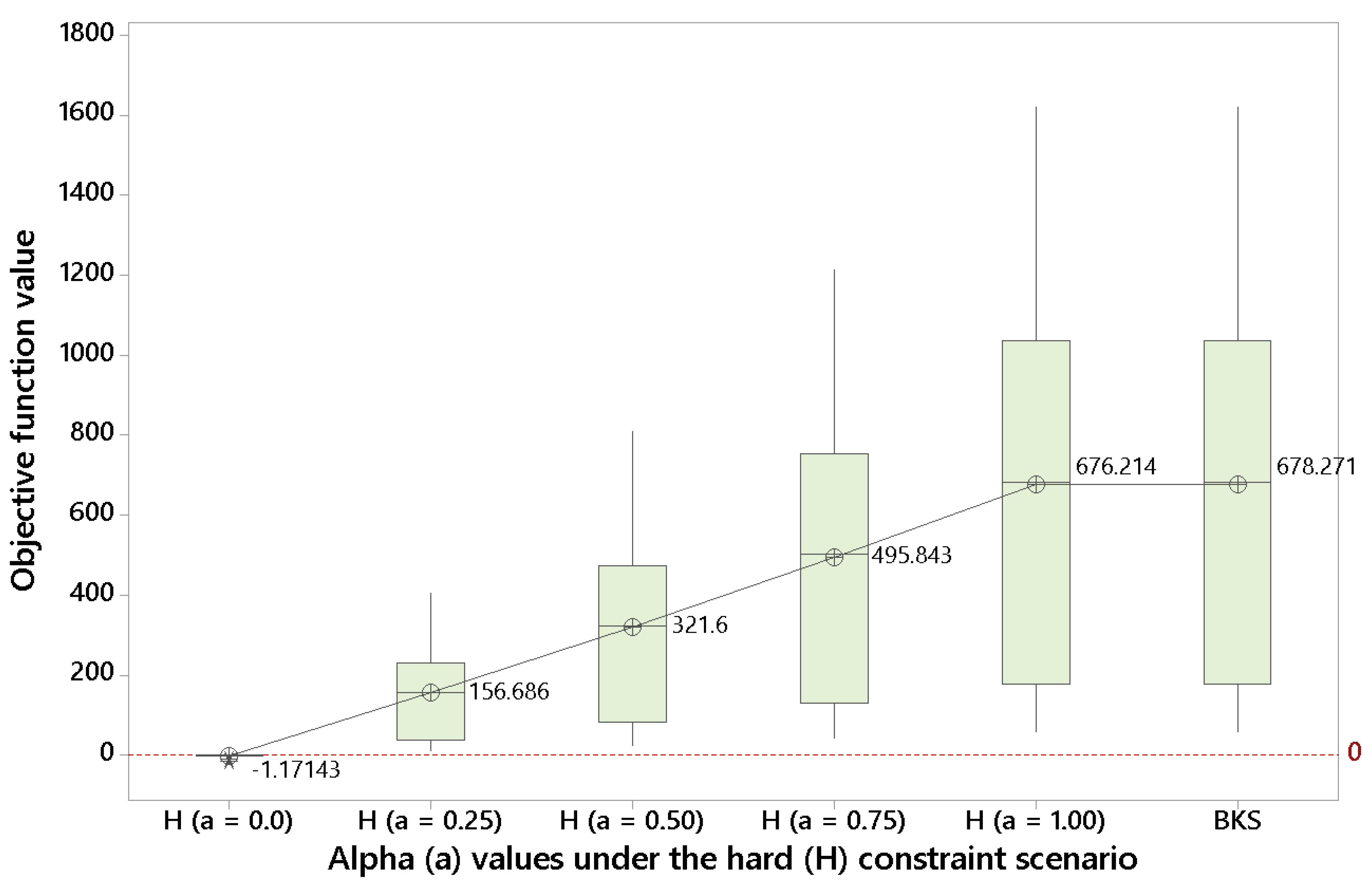According to the results that are shown in Figure 2, even using short computational times (a maximum time of 2 min. per instance was set), we obtain an average value of $675.2$, which is virtually the same as the one provided by the BKS ($678.3$). This illustrate the effectiveness of our approach when employed in the basic version of the TOP, which is a necessary step before solving the more advanced BONSTOP model. Figure 2 also shows that, as the value of $\alpha$ is reduced (i.e., less weight is given to the reward and more weight is assigned to the route balancing), the value of the objective function diminishes.

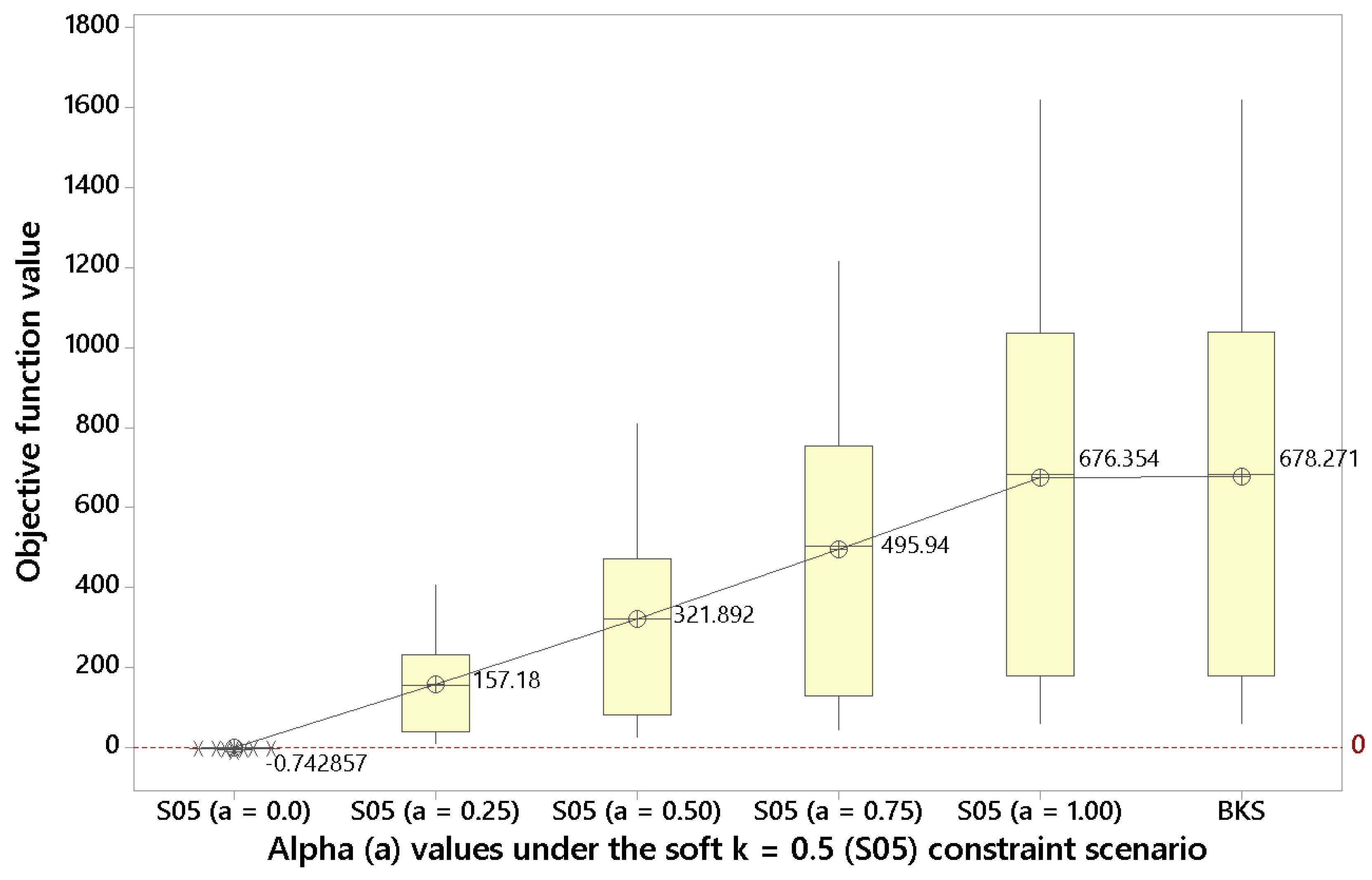
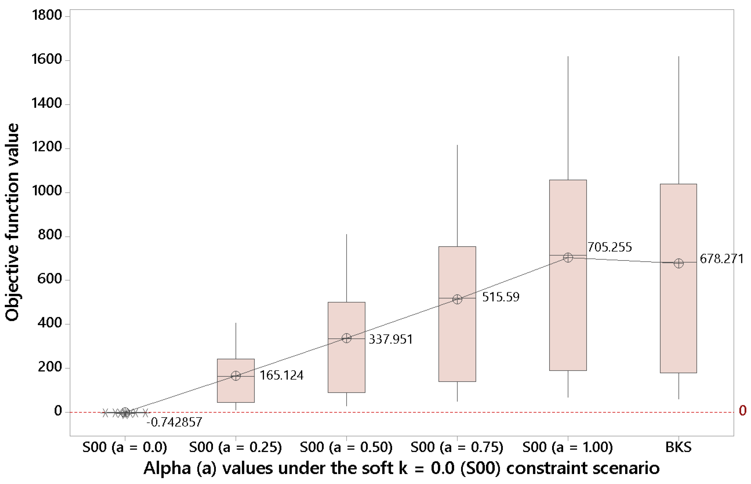
The next step is then solving the BONSTOP model when considering soft constraints. For $K=0.5$, Figure 3 shows that in this $S05$ soft constraint scenario it is possible to enhance the objective function for $\alpha =1$ by slightly violating the driving time constraints (i.e., the penalty cost incurred is overcompensated by the associated increase in total reward). Again, as $\alpha$ diminishes, the objective function value is reduced.

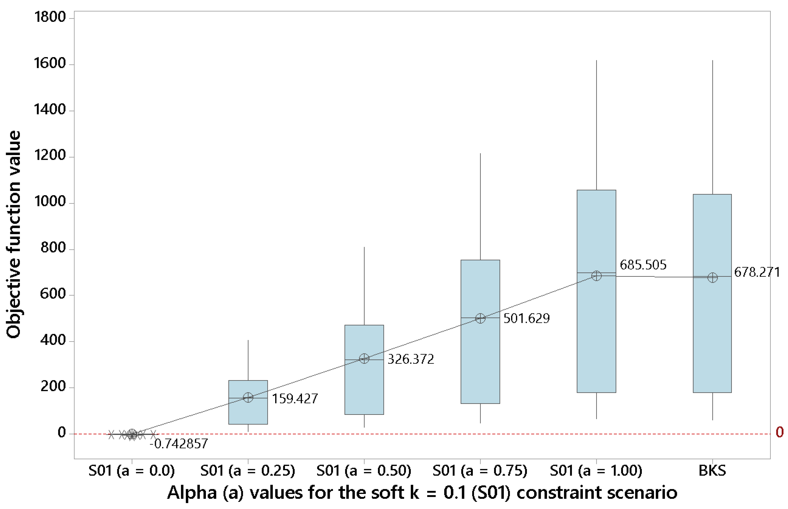
For soft constraint scenarios with a lower k ($k=0.1$ and $k=0.0$), Figure 4 and Figure 5 show—even clearer than before—that some benefits can be obtained by violating the driving time constraint when $\alpha =1$. This observation might be quite interesting for a manager, since, as discussed in the Introduction, in real-life is frequent to find constraints with a certain degree of flexibility.

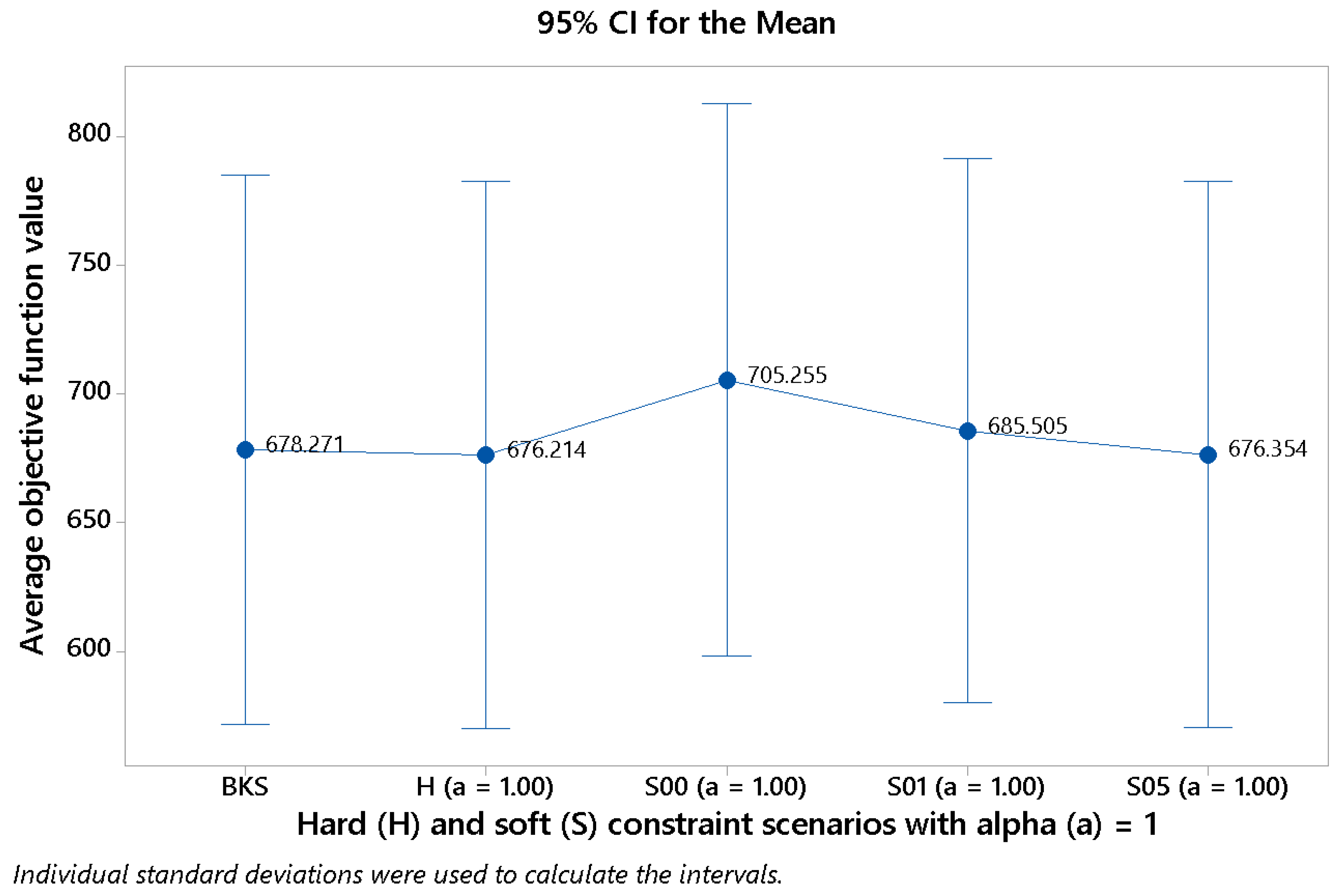
Finally, Figure 6 shows how the average value of the objective function varies as we move across different scenarios (with $\alpha =1$ in all cases). One can notice that, in effect, the more ‘soft’ the scenario, the higher the benefits that can be achieved. Hence, the average value is $705.3$ for scenario $S00$ (the most flexible one), while it reduces to $676.2$ for the hard scenario.

6. Conclusions

We studied a realistic non-smooth and bi-objective version of the team orienteering problem (TOP). Instead of assuming hard constraints on the maximum time a vehicle can drive, these driving-range limitations can be exceeded to some extent, i.e., they are soft constraints. However, when these constraints are violated, a penalty cost has to be paid. This penalty cost has to be considered in the weighted objective function, which aims at both minimizing total cost as well as to maximize the balance across routes (in terms of obtained reward) in the final solution. In our experiments, the penalty cost is given by a piece-wise function, which introduces a non-smooth component into the objective function. This, in turn, limits the efficiency of exact methods to solve the associated version of the TOP.

Therefore, a metaheuristic algorithm is proposed to solve this non-smooth TOP. It is based on a variable neighborhood search framework, which also integrates biased-randomization techniques. The numerical experiments illustrate the efficiency of our approach. It produces competitive solutions to the hard-constrained TOP. Moreover, for moderated levels of these penalty costs, our approach is able to provide solutions that outperform the hard-constrained optimal ones. In other words, we show that, under some circumstances, it might be worthy to exceed the driving-range limitations and cover the associated cost of this action. For example, a transportation company might be interested in paying some overtime to a driver if this allows the driver’s route to include new customers with high rewards that compensate the increase in cost. These numerical results support with data what we observed during the daily logistics planning that motivated this work: it was frequently worthy to extend somewhat the length of the planned routes—which were computed using hard constraints on the maximum time a driver can operate. By doing this, a noticeable increase in the added value of the sanitary items to be collected was usually obtained. Hence, the utilization of soft constraints, which has been rarely analyzed in the scientific literature on the TOP, is fully justified in real-life practice and it can lead to solutions outperforming the ones that are constrained by hard (and often unrealistic) thresholds. The experimental results also support the use of metaheuristic algorithms as an effective and efficient solving procedure to deal with the extraordinary complexity of the resulting optimization problem—which becomes non-smooth with the introduction of the piece-wise penalty cost functions associated with the soft constraints. This is especially the case when reasonably short computing times are required by managers and when different criteria are considered—e.g., reward maximization as well as balanced routing plans.

The current work still considers several simplifying assumptions, e.g.: both reward values as well as travel times are assumed to be deterministic and well-known in advance. Hence, no stochastic variables, reliability issues on the routing plans, or dynamic conditions are taken into account in our study. As potential research lines to be explored in future work, we can highlight the following ones: (i) the hybridization of our BR-VNS algorithm with the ECAM global optimization algorithm [40]—in particular, the former could be used to explore the solution space while the latter could help to intensify the search in a promising region; (ii) an extended version of the problem in which the optimal number of vehicles (fleet size) is also a decision variable to be set as part of the optimization process; and, (iii) the extension of our metaheuristic into a simheuristic [41], so it can also deal with stochastic customers’ rewards or travel times. The introduction of random travel times might arise complex reliability and availability issues on the planned routes and their assigned vehicles, especially when electric vehicles—with limited driving ranges—are employed. Simulation-based approaches can also help to deal with these issues [42].