Preview Tracking Control for Discrete-Time Multirate Systems: An Internal Model-Based Approach

Abstract

This paper investigates the preview tracking problem for discrete-time multirate systems under the scenario of the external signals with amplitude non-attenuation. Since the input and the state cannot be measured at the same time, the multirate system is first lifted into the single-rate system. Noting that the external signals are previewable and their amplitudes are unattenuated, an auxiliary system with preview information and a dynamic compensator with internal model are introduced, respectively. On this basis, the preview tracking problem can be converted to the output regulation problem of an augmented system with the aid of the state augmentation technique. Through verifying the solvability of the output regulation problem, the sufficient conditions and the corresponding controller with preview action and feedforward compensation are presented for the output regulation problem as well as the original problem. Finally, a numeric simulation result is provided to verify the validity of the proposed method.

1. Introduction

Multirate control system has attracted considerable attention due to a mount of sample requirements in many fields of industry. The analysis and synthesis for multirate systems originates in [1]. To date, various results have been developed for this issue [2,3,4,5,6,7,8,9,10]. In [2], a discrete-time state space equation was established for multirate systems, where four stability criteria were derived based on two forms of a transfer matrix related to the state space equation. In [3], proper algebraic conditions were provided to ensure the desired structural properties (such as, reachability, controllability and stabilizability, etc.) of multirate systems. If the saturated communication sequences are equidistant, multirate systems and networked control system with limited bandwidth were proved to be equivalent in [4], as a result, the related conclusions of the latter on controllability and stabilizability can be applied to analyze the former. In order to simulate the dynamic characteristics in sampling interval, two different discrete lifting techniques were applied in [5] to obtain the functional space model of the multirate control systems, then based on the definition of zeros and zero directions, the conditions for realizing asymptotic ripple-free tracking of multirate systems are provided.

Note that dual-rate control is suitable for the scenario that output data are sampled by a rate slower than that of control data sampling, [6] presented two adaptive control schemes for a dual-rate discretized continuous-time system. In addition, for dual-rate systems, the parameters of lifted single-rate systems were usually assumed to be known in most literature, [7] investigated the case of unknown parameters and developed an auxiliary model to identify the parameters of the lifted fast single-rate systems. In [8], the controller design for multirate systems were split into two steps, where the slow part was used to compute the control error and the fast part was applied to get the similar results with those achieved by the fast single-rate control. [9] considered the $H_{\infty }$ control synthesis problem for multirate systems and the solution of which was obtained by formulating that into a convex optimization problem. [10] studied the robust sample-data $H_{\infty }$ control problem for uncertain active vehicle suspension systems, in light of an input delay method, the original system was converted to a continuous-time system with a state delay. For other results of multirate systems, interested readers can also refer to References [11,12,13].

For many practical control systems, such as wind turbine control [14]; walking pattern generation for biped robots [15], the part (even full) of the external signals are usually known in advance for the system. Preview control theory comes along with the occurrence of such phenomenon, the core issue of which is to design a controller containing the future information to improve the response performance of the closed-loop system. To date, there have been many important advances in the theoretical research in this field. Tomizuka has done many groundbreaking works in this field, such as [16,17]. In [16], a method for designing tracking controller with preview information to minimize the optimality criterion is presented, where the reference signal is subject to Gaussian white noise. Based on the linear quadratic optimal control theory, a digital controller with error integral and preview compensation for discrete-time linear system is designed in [17]. In order to enrich the results of [17], the case of the unmeasurable state is further considered in [18]. It should be pointed out that if the reference signal incorporates the white noise or other random disturbances, the linear quadratic Gaussian (LQG) control technique will not be suitable for designing the optimal controller [19]. In addition, if the reference signal is treated as an external perturbation and the tracking problem is expressed as a H_∞ optimal control problem, the effect of the preview information will not be reflected. To this end, game theorem is adopted in [20] to study the finite time H_∞ tracking control problem. Furthermore, the discrete-time counterpart of [20] was investigated in [21]. Other relevant results for the H_∞ preview control can be also found in [22,23]. Moreover, by building an auxiliary system with preview information and augmenting it with the original system, the state feedback and the preview feedforward compensation in the controller can be designed in a unified way. Moreover, relevant results along this line can be referred to [24,25,26,27].

Currently, the preview control for multirate systems has also been extensively studied. In [28,29], the multirate system subject to input delay and state delay were transformed into a single-rate system without time-delay by discrete lifting technique, which simplified the problem significantly. Recently, based on the above results, optimal preview control problem for descriptor multirate systems was solved in [30,31]. Moreover, the cases of dual-rate systems and uncertain multirate systems have also been considered in [32,33], respectively. Note that, in the theoretical research of the preview control for multirate system, it is assumed that the reference signal tends to be a constant vector (or scalar) as time approaches infinity. However, many reference signals with unattenuated amplitudes, for instant sinusoidal signal, do not meet such assumption. Recently, using the distributed internal model principle, the cooperative preview tracking problem of multi-agent system with undamped amplitude was investigated in [34].

Inspired by the research method of [34], this study intends to consider the preview control problem of multirate systems with non-decreased amplitude reference signal by introducing the internal model compensator. Consequently, the preview tracking problem is processed via transforming it into an output regulation problem of an augmented system. The innovations are summarized as follows:

(1)

The preview control problem of multirate systems is further improved by considering the scenario of amplitude non-decaying reference signal;

(2)

The stabilizability and detectability of the augmented systems are proved strictly, which guarantees the existence and uniqueness of solutions of Riccati equation and Sylvester equation;

(3)

The asymptotical tracking conditions for existing an multirate controller with error integral, internal model compensation and preview feedforward compensation are presented.

Notations: Let ${ℛ}^n$ and ${ℛ}^{n\times m}$ be the $n$-dimensional Euclidean space and the $n\times m$ matrix space, respectively. $I_n$ denotes the $n\times n$ identity matrix. $\mathsf{\Lambda }(S)$ represents the spectrum of the matrix $S$, i.e., $\left\{\lambda |\det (\lambda I-S)=0\right\}$. ‘iff’ means ‘if and only if’. $diag\{\cdots \}$ stands for a diagonal matrix. $Q>0$ denotes that $Q$ is a symmetric positive definite matrix. ‘$\cup$’ means the union of different sets; ‘$A\otimes B$’ represents the Kronecker product of matrices $A$ and $B$.

2. Problem Formulation

Consider a discrete-time system

$$\{\begin{array}{l}x(k+1)=Ax(k)+Bu(k)+Dw(k)\hfill \\ y(k)=Cx(k)\hfill \end{array}$$

(1)

where $x(k)\in {ℛ}^n$, $u(k)\in {ℛ}^m$, $w(k)\in {ℛ}^p$ and $y(k)\in {ℛ}^q$ are the state, the control input, the disturbance and the measured output, respectively. $A\in {ℛ}^{n\times n}$, $B\in {ℛ}^{n\times m}$, $C\in {ℛ}^{q\times n}$ and $D\in {ℛ}^{n\times p}$ are constant matrices.

Additionally, assume that $r(k)\in {ℛ}^q$ is a reference signal, which is generated by the following system:

$$\{\begin{array}{l}v(k+1)=S_{1}v(k)\hfill \\ r(k)=F_{1}v(k)\hfill \end{array}$$

(2)

Moreover, suppose that the disturbance signal $w(k)$ is produced by

$$w(k+1)=S_{2}w(k)$$

(3)

where $v(k)\in {ℛ}^d$ denotes the state of system (2), $S_1\in {ℛ}^{d\times d}$, $S_2\in {ℛ}^{p\times p}$ and $F_1\in {ℛ}^{q\times d}$ are constant matrices.

To facilitate the description of the problem, the following assumptions associated with the Equations (1)–(3) are required.

Hypothesis 1 (H1).

$x(k)$ and $y(k)$ can be measured only at $k=Ni$, where $i=0,1,\cdots$ and $N\in Z^{+}$.

Hypothesis 2 (H2).

$(A,B)$ is stabilizable and $(C,A)$ is detectable.

Hypothesis 3 (H3).

$S_1$ and $S_2$ have no eigenvalue inside the unit circle in the complex plane.

Hypothesis 4 (H4).

both of $r(k)$ and $w(k)$ are previewable, and the preview lengths are $h_r=s_{r}N$ and $h_d=s_{d}N$, respectively, which means that values of $r(k+1)$, $r(k+2),$ $\cdots$, $r(k+h_r)$ and $w(k+1)$, $w(k+2)$,.., $w(k+h_d)$ are known beforehand. Furthermore, $s_r$ and $s_d$ are nonnegative integers.

Remark 1.

For assumption H4, there are many studies in the literature talking about the application of previewable reference signal, such as [14,15]. In what follows, we take the active suspension of the vehicle as an example to explain the application and significance of disturbance previewable information in real systems. As shown in [35], moving objects such as vehicles and mobile robots will vibrate when driving on uneven roads. For the vibration damping system of the mobile objects, the unevenness of the road is actually a kind of external disturbance and a natural idea is to use the active suspension device to control vibration. That is to say, the road conditions, such as concavities and convexities, in front of the mobile objects are detected by some sensors, and the collected data can be viewed as preview information and applied in the control of the suspension device. Since the front or future road information are known in advance, there is enough time for the suspension device to choose suitable control policy to against vibration.

Define the following error signal:

$$e(k)=y(k)-r(k)=Cx(k)-r(k)$$

(4)

This study aims to design a controller with preview feedforward compensation based on internal model principle, which achieves $\underset{t\to \infty }{\lim }e(k)=0$ when $t\to +\infty$.

3. Discrete Lifting and Problem Translation

In general, state feedback takes the form of $u(k)=Kx(k)+v(k)$, where $v(k)$ is a new assistant input. According to H1, state vector $x(k)$ and output vector $y(k)$ only obtain sampling value at $k=iN$ ($i=0,1,\cdots$ and $N\in Z^{+}$). However, the input vector $u(k)$ has sampled data $N$ times rapidly. Therefore, $x(k)$ cannot be used in state feedback when $k\ne iN$, which brings difficulties to design a controller for multirate systems (1).

Discrete lifting technique can usually be applied to transform the multirate system into the single-rate system. The main method is to obtain the sampling values of each variable at the same time by lifting the dimension of the signal. For the convenience of subsequent derivation, we give the following lifting process according to (1):

$$x(iN+2)=Ax(iN+1)+Bu(iN+1)+Dw(iN+1)$$

(5)

Using (1), Formula (5) can be further written as

$$\begin{array}{ll}x(iN+2)\hfill & =Ax(iN+1)+Bu(iN+1)+Dw(iN+1)\hfill \\ & =A[Ax(iN)+Bu(iN)+Dw(iN)]+Bu(iN+1)+Dw(iN+1)\hfill \\ & =A^{2}x(iN)+[ABu(iN)+Bu(iN+1)]+[ADw(iN)+Dw(iN+1)]\hfill \end{array}$$

(6)

The rest can be done in the same procedure, that is

$$\begin{array}{ll}x(iN+j)\hfill & =A^{j}x(iN)+[A^{j-1}Bu(iN)+A^{j-2}Bu(iN+1)+\cdots \hfill \\ & +Bu(iN+j-1)]+[A^{j-1}Dw(iN)+A^{j-2}Dw(iN+1)+\cdots \hfill \\ & +Dw(iN+j-1)]\hfill \end{array}$$

(7)

where $j=1,2,\cdots ,N$. Assume that

$$\begin{array}{cc}X(i)=x(iN),& Y(i)=\left[\begin{array}{c}y(iN)\\ y(iN+1)\\ ⋮\\ y(iN+N-1)\end{array}\right],\\ U(i)=\left[\begin{array}{c}u(iN)\\ u(iN+1)\\ ⋮\\ u(iN+N-1)\end{array}\right],& W(i)=\left[\begin{array}{c}w(iN)\\ w(iN+1)\\ ⋮\\ w(iN+N-1)\end{array}\right].\end{array}$$

then according to Formulas (5)–(7), the single-rate system is obtained:

$$\{\begin{array}{l}X(i+1)=A_{1}X(i)+B_{1}U(i)+D_{1}W(i)\hfill \\ Y(i)=C_{1}X(i)+B_{2}U(i)+D_{2}W(i)\hfill \end{array}$$

(8)

with

$$\begin{gathered} A_1=A^N,C_1={\left[\begin{array}{ccccc}{C}^T& {(CA)}^T& {(C{A}^2)}^T& \cdots & {(C{A}^{N-1})}^T\end{array}\right]}^T, \\ {B}_1=\left[\begin{array}{cccc}{A}^{N-1}B& \cdots & AB& B\end{array}\right],D_1=\left[\begin{array}{cccc}{A}^{N-1}D& \cdots & AD& D\end{array}\right], \\ {B}_2=\left[\begin{array}{ccccc}0& & & & \\ CB& 0& & & \\ CAB& CB& 0& & \\ ⋮& \ddots & \ddots & \ddots & \\ C{A}^{N-2}B& \cdots & CAB& CB& 0\end{array}\right],D_2=\left[\begin{array}{ccccc}0& & & & \\ CD& 0& & & \\ CAD& CD& 0& & \\ ⋮& \ddots & \ddots & \ddots & \\ C{A}^{N-2}D& \cdots & CAD& CD& 0\end{array}\right] \end{gathered}$$

In addition, for the error signal $e(iN)=y(iN)-r(iN)$, set

$$E(i)=\left[\begin{array}{c}e(iN)\\ e(iN+1)\\ ⋮\\ e(iN+N-1)\end{array}\right],R(i)=\left[\begin{array}{c}r(iN)\\ r(iN+1)\\ ⋮\\ r(iN+N-1)\end{array}\right]$$

then, it follows from the system (7) that

$$E(i)=C_{1}X(i)+B_{2}U(i)+D_{2}W(i)-R(i)$$

(9)

For system (8), $(A_1,B_1)$ was verified to be stabilizable in [28]. Using the duality principle, it can be easily verified that: if $(C,A)$ is detectable, then $(C_1,A_1)$ is detectable. Moreover, to address the original problem, the following assumption is necessary for system (8).

Hypothesis 5 (H5).

For any $\lambda \in \mathsf{\Lambda }(S_1)\cup \mathsf{\Lambda }(S_2)$, $\left[\begin{array}{cc}\lambda I-A_1& B_1\\ C_1& B_2\end{array}\right]$ is assumed to be of full row rank. Furthermore, if $1\notin \mathsf{\Lambda }(S_1)\cup \mathsf{\Lambda }(S_2)$, the above rank condition also holds for $\lambda =1$.

Next, we employ the state augmentation technique to establish an augmented system with respect to the tracking error, state variable difference and preview information. A basic consideration is that if a suitable controller is designed to make the closed-loop augmented system asymptotically stable, then as the state component, the tracking error can be asymptotically stabilized to zero. Simultaneously, the preview information will be involved in the controller by means of the state feedback.

Note that $A_{1}X(i)$, $B_{1}U(i)$ and $D_{1}W(i)$ are essentially vectors in (8) and so is $A_{1}X(i)+B_{1}U(i)+D_{1}W(i)$. Then, utilizing the first-order forward difference operator

$$\Delta \eta (i)=\eta (i+1)-\eta (i)$$

(10)

to both sides of the first equation of system (8), we have

$$\begin{gathered} \Delta X(i+1)=\Delta [A_{1}X(i)+B_{1}U(i)+D_{1}W(i)] \\ =[A_{1}X(i+1)+B_{1}U(i+1)+D_{1}W(i+1)]-[A_{1}X(i)+B_{1}U(i)+D_{1}W(i)] \\ =A_1[X(i+1)-X(i)]+B_1[U(i+1)-U(i)]+D_1[W(i+1)-W(i)] \\ =A_1\Delta X(i)+B_1\Delta U(i)+D_1\Delta W(i) \end{gathered}$$

Moreover, taking the same operation for (9) yields

$$\begin{gathered} \Delta E(i)=\Delta [C_{1}X(i)+B_{2}U(i)+D_{2}W(i)-R(i)] \\ \begin{array}{c}=[C_{1}X(i+1)+B_{2}U(i+1)+D_{2}W(i+1)-R(i+1)]\\ -[C_{1}X(i)+B_{2}U(i)+D_{2}W(i)-R(i)]\end{array} \\ =C_1\Delta X(i)+B_2\Delta U(i)+D_2\Delta W(i)-\Delta R(i) \end{gathered}$$

Combining the above two formulas gives

$$\{\begin{array}{l}\Delta X(i+1)=A_1\Delta X(i)+B_1\Delta U(i)+D_1\Delta W(i)\hfill \\ \Delta E(i)=C_1\Delta X(i)+B_2\Delta U(i)+D_2\Delta W(i)-\Delta R(i)\hfill \end{array}$$

(11)

Denote $\overline{X}(i)=\left[\begin{array}{c}E(i)\\ \Delta X(i)\end{array}\right]$, $\overline{A}=\left[\begin{array}{cc}I& C_1\\ 0& A_1\end{array}\right]$, $\overline{B}=\left[\begin{array}{c}{B}_2\\ B_1\end{array}\right]$, $\overline{E}=\left[\begin{array}{c}{D}_2\\ D_1\end{array}\right]$, $\overline{F}=\left[\begin{array}{c}-I\\ 0\end{array}\right]$, then the above equation can be written as

$$\overline{X}(i+1)=\overline{A}\overline{X}(i)+\overline{B}\Delta U(i)+\overline{E}\Delta W(i)+\overline{F}\Delta R(i)$$

(12)

Note that the reference signal and disturbance signal are previewable and the preview lengths are $h_r=s_{r}N$ and $h_d=s_{d}N$, respectively. Based on the construction of $\Delta R(i)$ and $\Delta W(i)$, we know that the future values $\Delta R(i)$, $\Delta R(i+1)$, $\cdots$, $\Delta R(i+s_r-1)$ and $\Delta W(i)$, $\Delta W(i+1)$, $\cdots$, $\Delta W(i+s_d-1)$ are available for system (12). In order to design a controller with preview information, the following auxiliary systems are constructed,

$$X_r(i+1)=A_r{X}_r(i)+B_r\Delta R(i+s_r)$$

(13)

$$X_w(i+1)=A_w{X}_w(i)+B_w\Delta W(i+s_d)$$

(14)

where

$$\begin{gathered} X_r(i)=\left[\begin{array}{c}\Delta R(i)\\ \Delta R(i+1)\\ ⋮\\ \Delta R(i+s_r-1)\end{array}\right],X_w(i)=\left[\begin{array}{c}\Delta W(i)\\ \Delta W(i+1)\\ ⋮\\ \Delta W(i+s_d-1)\end{array}\right],A_r={\left[\begin{array}{cccc}0& I& & \\ & 0& \ddots & \\ & & \ddots & I\\ & & & 0\end{array}\right]}_{q{s}_{r}N\times q{s}_{r}N} \\ {A}_w={\left[\begin{array}{cccc}0& I& & \\ & 0& \ddots & \\ & & \ddots & I\\ & & & 0\end{array}\right]}_{p{s}_{d}N\times p{s}_{d}N},B_r={\left[\begin{array}{c}0\\ ⋮\\ 0\\ I\end{array}\right]}_{q{s}_{r}N\times qN},B_w={\left[\begin{array}{c}0\\ ⋮\\ 0\\ I\end{array}\right]}_{p{s}_{r}N\times pN} \end{gathered}$$

By considering the Formulas (12)–(14), an augmented system is obtained as follows,

$$\{\begin{array}{l}\widehat{X}(i+1)=\widehat{A}\widehat{X}(i)+\widehat{B}\Delta U(i)+{\widehat{B}}_r\Delta R(i+s_r)+{\widehat{B}}_w\Delta W(i+s_d)\hfill \\ E(i)=\widehat{C}\widehat{x}(i)\hfill \end{array}$$

(15)

where $\widehat{X}(i)=\left[\begin{array}{c}\overline{X}(i)\\ X_r(i)\\ X_w(i)\end{array}\right]$, $\widehat{A}=\left[\begin{array}{ccc}\overline{A}& \widehat{F}& \widehat{E}\\ 0& A_r& 0\\ 0& 0& A_w\end{array}\right]$, $\widehat{B}=\left[\begin{array}{c}\overline{B}\\ 0\\ 0\end{array}\right]$, ${\widehat{B}}_r=\left[\begin{array}{c}0\\ B_r\\ 0\end{array}\right]$, ${\widehat{B}}_w=\left[\begin{array}{c}0\\ 0\\ B_w\end{array}\right]$, $\widehat{F}=[\begin{array}{cccc}\overline{F}& 0& \cdots & 0\end{array}]$, $\widehat{E}=[\begin{array}{cccc}\overline{E}& 0& \cdots & 0\end{array}]$. In addition, $E(i)=\widehat{C}\widehat{X}(i)$ represents the observation equation with $\widehat{C}={\left[\begin{array}{cccc}I& 0& 0& 0\end{array}\right]}_{qN\times (qN+n+q{s}_{r}N+p{s}_{d}N)}$.

Remark 2.

The benefits of constructing the augmented system (15) are twofold: (1) Since the future values of the reference and disturbance signals are incorporated in the state vector of the augmented system (15), the preview feedforward compensation can be realized through state feedback; (2) The augmented system can deal with the circumstance of existing preview information or not simultaneously, which makes the design method proposed in this study more applicable.

In what follows, by exploiting systems (2) and (3), $\Delta R(i+s_r)$ and $\Delta W(i+s_d)$ can be rewritten as

$$\{\begin{array}{c}\Delta R(i+s_r)=(I_N\otimes F_1{S}_1^{s_{r}N})\Delta V(i)\\ \Delta W(i+s_d)=(I_N\otimes S_2^{s_{d}N})\Delta W(i)\end{array}$$

(16)

Here, $V^T(i)=\left[\begin{array}{cccc}{v}^T(iN)& v^T(iN+1)& \cdots & v^T(iN+N-1)\end{array}\right]$ and $W(i)$ was defined in Formula (8). Furthermore, by virtue of the relationships among $\Delta R(i)$, $\Delta W(i)$, $\Delta X_r(i)$ and $\Delta X_w(i)$, as well as the Formula (16), the augmented system (15) can be described as

$$\{\begin{array}{l}\widehat{X}(i+1)=\widehat{A}\widehat{X}(i)+\widehat{B}\Delta U(i)+\tilde{B}\Delta \tilde{w}(i)\hfill \\ E(i)=\widehat{C}\widehat{X}(i)\hfill \end{array}$$

(17)

where $\tilde{B}=\left[\begin{array}{cc}{\widehat{B}}_r(I_N\otimes F_1{S}_1^{s_{r}N})& {\widehat{B}}_w(I_N\otimes S_2^{s_{d}N})\end{array}\right]$, $\tilde{w}(i)={\left[\begin{array}{cc}V{(i)}^T& W{(i)}^T\end{array}\right]}^T$.

Consider the non-decreased amplitude of $r(k)$ and $w(k)$, thus $\Delta \tilde{w}(i)$ is an unstable signal. To achieve the control goal of zero-error tracking, the internal model principle will be applied to solve the problem in the sequence. Denote $S=diag{(S_1,S_2)}_{p+q}$, the definition of the least $p+q$-fold internal model of the matrix $S$ is introduced first.

Definition 1

[36,37]. If $(G_1,G_2)$ admits the following form

$$G_1={\left[\begin{array}{cccc}\beta & 0& \cdots & 0\\ 0& \beta & \cdots & 0\\ ⋮& ⋮& \ddots & ⋮\\ 0& 0& \cdots & \beta \end{array}\right]}_{[(p+q)l]\times (p+q)l},G_2={\left[\begin{array}{cccc}\sigma & 0& \cdots & 0\\ 0& \sigma & \cdots & 0\\ ⋮& ⋮& \ddots & ⋮\\ 0& 0& \cdots & \sigma \end{array}\right]}_{[(p+q)l]\times (p+q)}$$

where $\beta$ is a $l\times l$ constant matrix and $\sigma$ is a constant column vector with the dimension of $l$ and

(1) 

the pair $(\beta ,\sigma )$ is completely controllable;

(2) 

the characteristic polynomial and the minimal polynomial of $\beta$, as well as the minimal polynomial of $S$ are equivalent,

then $(G_1,G_2)$ is said to incorporate a least $p+q$-fold internal model of the matrix $S$.

Considering the characteristic of the multirate system, a dynamic compensator is proposed based on the least $p+q$-fold internal model and tracking error $e(k)$, $k=iN$.

$$x_c(iN+1)=G_1{x}_c(iN)+G_{2}e(iN)$$

By employing the discrete lifting technique to the compensator mentioned above, the following dynamic state feedback for system (17) is constructed,

$$\{\begin{array}{l}{X}_c(i+1)={\overline{G}}_1{X}_c(i)+{\overline{G}}_{2}E(i)\hfill \\ \Delta U(i)=K_1\widehat{X}(i)+K_2{X}_c(i)\hfill \end{array}$$

(18)

where ${\overline{G}}_1\in {ℛ}^{[(p+q)lN]\times [(p+q)lN]}$, ${\overline{G}}_2\in {ℛ}^{[(p+q)lN]\times [(p+q)N]}$, moreover, $X_c(i)$, ${\overline{G}}_1$ and ${\overline{G}}_2$, respectively, have the form of

$$X_c(i)=\left[\begin{array}{c}{x}_c(iN)\\ x_c(iN+1)\\ ⋮\\ x_c(iN+N-1)\end{array}\right],{\overline{G}}_1=\left[\begin{array}{cccc}{G}_1& & & \\ & G_1& & \\ & & \ddots & \\ & & & G_1\end{array}\right],{\overline{G}}_2=\left[\begin{array}{cccc}{G}_2& & & \\ & G_2& & \\ & & \ddots & \\ & & & G_2\end{array}\right]$$

Substituting the dynamic feedback (18) into system (17) and setting $\tilde{X}(i)={\left[\begin{array}{cc}{\widehat{X}}^T(i)& X_c^T(i)\end{array}\right]}^T$ yield the following closed-loop system

$$\{\begin{array}{l}\tilde{X}(i+1)=A_c\tilde{X}(i)+B_c\Delta \tilde{w}(i)\hfill \\ \Delta \tilde{w}(i+1)=\tilde{S}\Delta \tilde{w}(i)\hfill \\ E(i)=C_c\tilde{X}(i)\hfill \end{array}$$

(19)

where

$$\begin{gathered} A_c=\left[\begin{array}{cc}\widehat{A}+\widehat{B}{K}_1& \widehat{B}{K}_2\\ {\overline{G}}_2\widehat{C}& {\overline{G}}_1\end{array}\right],B_c=\left[\begin{array}{c}\tilde{B}\\ 0\end{array}\right],\tilde{S}=\left[\begin{array}{cc}{\tilde{S}}_1& \\ & {\tilde{S}}_2\end{array}\right], \\ {C}_c=\left[\begin{array}{cc}\widehat{C}& 0\end{array}\right],{\tilde{S}}_1=I_N\otimes S_1^N,{\tilde{S}}_2=I_N\otimes S_2^N \end{gathered}$$

Through the above procedure, the preview tracking problem of the multirate system (1) is eventually formulated as the output regulation problem with respect to system (19). According to [36], the latter problem is solvable provided that the dynamic feedback (18) makes the closed loop system (19) satisfy the following two properties:

(1)

homogeneous system

$$\begin{array}{l}\tilde{X}(i+1)=A_c\tilde{X}(i)\hfill \end{array}$$

(20)

is exponentially stable;

(2)

for any initial condition ${\tilde{X}}_c(0)$ and $\tilde{w}(i)$, ${\lim }_{i\to \infty }E(i)=0$ holds.

Note that the form of $E(i)$ and the sampling time $k=iN$, if the controller $\Delta U(i)$ satisfies the property 2), then it follows that ${\lim }_{k\to \infty }e(k)=0$. That is to say, $\Delta U(i)$ solves the preview tracking problem of the multirate system (1). Correspondingly, by the definition of the difference operator $\Delta$, the control law $U(i)$ can be derived through iterative calculation, which also contains the specific expression of $u(k+j)$ $j=0,1,\cdots ,N-1$.

Remark 3.

$({\overline{G}}_1,{\overline{G}}_2)$ in dynamic feedback (18) can be attained by the following procedure. Based on the Definition 1, the minimum polynomial of $S$ is $p(\lambda )={\lambda }^1+{\alpha }_{l-1}{\lambda }^{l-1}+\cdots +{\alpha }_1\lambda +{\alpha }_0$, then $p(\lambda )$ is also the minimum polynomial of $\beta$. Since $(G_1,G_2)$ is completely controllable, the minimum polynomial corresponding to its first controllable canonical form is just $p(\lambda )$. On this basis, $(\beta ,\sigma )$ can be established as follows,

$$\beta =\left[\begin{array}{ccccc}0& & 1& & \\ ⋮& & & \ddots & \\ 0& & & & 1\\ -{\alpha }_0& & -{\alpha }_1& \cdots & -{\alpha }_{l-1}\end{array}\right],\sigma =\left[\begin{array}{c}0\\ ⋮\\ 0\\ 1\end{array}\right]$$

4. Main Results

In this section, sufficient conditions are given to ensure the solvability of the output regulation problem. Meanwhile, the controller needed for the output regulation problem and the original problem will be designed through the optimal control method. Before giving the main results, we first introduce the following lemma,

Lemma 1

[37]. Under H3, assume that $(G_1,G_2)$ incorporates a minimal $p+q$-fold internal model of the matrix $S$. If $\left[\begin{array}{cc}\widehat{A}& \widehat{B}\\ G_2\widehat{C}& G_1\end{array}\right]$ is exponentially stable for the matrices $\widehat{A}$, $\widehat{B}$ and $\widehat{C}$ with appropriate dimension. Then, for any matrices $\widehat{E}$ and $\widehat{F}$, the following regulation equation

$$\{\begin{array}{l}X{A}_v=\widehat{A}X+\widehat{B}Z+\widehat{E}\hfill \\ Z{A}_v=G_{1}Z+G_2(\widehat{C}X+\widehat{F})\hfill \end{array}$$

(21)

exists a unique solution pair (X, $Z$). Moreover, $X$ also satisfies

$$\widehat{C}X+\widehat{F}=0$$

(22)

The following theorem gives sufficient conditions for implementing the output regulation of the system (19).

Theorem 1.

Suppose that $(G_1,G_2)$ incorporates a minimal ($p+q$)-fold internal model of the matrix $S$. If $A_c$ is stable, then the dynamic feedback controller (18) makes the system (19) achieve the output regulation.

Proof. 

According to [36], the asymptotical stability of the system (20) implies its exponential stability. Therefore, if the matrix $A_c$ is stable, then the property 1) holds. Next, we prove ${\lim }_{t\to \infty }E(i)=0$. □

In fact, it follows from the basic knowledge of linear algebra that the least polynomial of $\beta$ is equal to the least common multiple with respect to the least polynomials of $S_1$ and $S_2$. Hence the least polynomial of $G_1^N$ is the least common multiple corresponding to the least polynomial of $S_1^N$ and $S_2^N$, which implies that the least polynomial of $G_1^N$ is equal to that of $\tilde{S}$. In addition, it is apparent that $({\overline{G}}_1,{\overline{G}}_2)$ is completely controllable. Recalling the Definition 1, it follows that $({\overline{G}}_1,{\overline{G}}_2)$ incorporates a minimal $(p+q)N$-fold internal model of the matrix $\tilde{S}$. Under the condition that $A_c$ is stable, let $\widehat{E}=\tilde{B}$, $\widehat{F}=0$, according to Lemma 1, there exists a unique solution pair $(X,Z)$ for the following regulation Equation

$$\{\begin{array}{l}X\tilde{S}=(\widehat{A}+\widehat{B}{K}_1)X+\widehat{B}{K}_{2}Z+\tilde{B}\hfill \\ Z\tilde{S}={\overline{G}}_{1}Z+{\overline{G}}_2\widehat{C}X\hfill \end{array}$$

(23)

with $X$ satisfying $\widehat{C}X=0$.

Let $\mathsf{\Gamma }={[X^T,Z^T]}^T$ and take the coordinate transformation ${\tilde{X}}_c(i)=\tilde{X}(i)-\mathsf{\Gamma }\Delta \tilde{w}(i)$, using system (19) and regulation Equation (23) gives

$$\begin{array}{ll}{\tilde{X}}_c(i+1)\hfill & =\tilde{X}(i+1)-\mathsf{\Gamma }\Delta \tilde{w}(i+1)\hfill \\ & =A_c\tilde{X}(i)+B_c\Delta \tilde{w}(i)-\mathsf{\Gamma }\tilde{S}\Delta \tilde{w}(i)\hfill \\ & =A_c{\tilde{X}}_c(i)+(A_c\mathsf{\Gamma }+B_c-\mathsf{\Gamma }\tilde{S})\Delta \tilde{w}(i)\hfill \\ & =A_c{\tilde{X}}_c(i)\hfill \end{array}$$

(24)

Due to the fact that $A_c$ is stable, then ${\tilde{X}}_c(i)$ asymptotically stabilizes to the origin. Performing the coordinate transformation to $E(i)=C_c\tilde{X}(i)$, we have

$$E(i)=C_c\tilde{X}(i)=C_c{\tilde{X}}_c(i)+C_c\mathsf{\Gamma }\Delta \tilde{w}(i)=C_c{\tilde{X}}_c(i)+\widehat{C}X\Delta \tilde{w}(i)$$

(25)

Since $\widehat{C}X=0$, the result of the property 2) is obvious. Q.E.D.

From Theorem 1, it can be observed that the key to achieve the output regulation is the stability of $A_c$. Note that

$$A_c=\left[\begin{array}{cc}\widehat{A}& 0\\ {\overline{G}}_2\widehat{C}& {\overline{G}}_1\end{array}\right]+\left[\begin{array}{c}\widehat{B}\\ 0\end{array}\right]\left[\begin{array}{cc}{K}_1& K_2\end{array}\right]$$

Denote $A_0=\left[\begin{array}{cc}\widehat{A}& 0\\ {\overline{G}}_2\widehat{C}& {\overline{G}}_1\end{array}\right]$, $B_0=\left[\begin{array}{c}\widehat{B}\\ 0\end{array}\right]$. Based on $(A_0,B_0)$, the system (20) can be redescribed as follows,

$$\tilde{X}(i+1)=A_0\tilde{X}(i)+B_0\Delta U(i)$$

(26)

Corresponding to the tracking problem, we introduce the following quadratic performance index function for system (26).

$$J={\displaystyle \sum _{i=1}^{\infty }\left[E^T(i)Q_{E}E(i)+X_c{}^T(i)Q_C{X}_c(i)+\Delta U^T(i)H\Delta U^T(i)\right]}$$

(27)

where $Q_E=diag(\underset{N}{\underbrace{Q_e,Q_e,\cdots ,Q_e}})$, $Q_C=diag(\underset{N}{\underbrace{Q_c,Q_c,\cdots ,Q_c}})$, $H=diag(\underset{N}{\underbrace{R,R,\cdots ,R}})$ and $Q_e\in {ℛ}^{q\times q}$, $Q_c\in {ℛ}^{(p+q)l\times (p+q)l}$, $R\in {ℛ}^{m\times m}$.

Rewrite (27) as

$$J={\displaystyle \sum _{i=1}^{\infty }\left[{\tilde{X}}^T(i)\tilde{Q}\tilde{X}(i)+\Delta U^T(i)H\Delta U^T(i)\right]}$$

(28)

with $\tilde{Q}=diag(Q_E,0,Q_C)$, then utilizing the conclusions of optimal control [38] gives the following result.

Lemma 2.

If $(A_0,B_0)$ is stabilizable and $({\tilde{Q}}^{1/2},A_0)$ is detectable, the optimal control input of the system (27) with the minimal performance index function (28) is

$$\Delta U(i)=\tilde{K}\tilde{X}(i)$$

(29)

where $\tilde{K}=-{(H+B_0^{T}P{B}_0)}^{-1}{B}_0^{T}P{A}_0$. $P$ is a symmetric positive semidefinite matrix satisfying the following discrete algebraic Riccati equation

$$P=\tilde{Q}+A_0{}^{T}P{A}_0-A_0{}^{T}P{B}_0{(H+B_0{}^{T}P{B}_0)}^{-1}{B}_0{}^{T}P{A}_0$$

(30)

and $A_0+B_0\tilde{K}$ is stable.

In order to ensure Lemma 2, it is necessary to verify the stabilizability of $(A_0,B_0)$ and the detectability of $({\tilde{Q}}^{1/2},A_0)$.

Theorem 2.

If H2, H3 and H5 hold, then $(A_0,B_0)$ is stabilizable.

Proof. 

From the PBH rank criterion [39], the stabilizability of $(A_0,B_0)$ will be proved if the matrix $\left[\begin{array}{cc}sI-A_0& B_0\end{array}\right]$ is shown to be of full row rank for any $\left|s\right|\ge 1$. In accordance with the structures of $A_0$ and $B_0$, $\left[\begin{array}{cc}sI-A_0& B_0\end{array}\right]$ can be expanded as

Because sI is nonsingular ($\left|s\right|\ge 1$), Using $sI$ to perform the row elementary transformation on the above formula yields

$$rank\left[\begin{array}{cc}sI-A_0& B_0\end{array}\right]=q{s}_{r}N+p{s}_{d}N+rankM(s)$$

(31)

where

$$M(s)=\left[\begin{array}{cccc}(s-1)I& -C_1& 0& B_2\\ 0& sI-A_1& 0& B_1\\ -{\overline{G}}_2& 0& sI-{\overline{G}}_1& 0\end{array}\right]$$

(32)

Therefore, it suffices to prove that $M(s)$ has full row rank for any $\left|s\right|\ge 1$ under the given conditions.□

For the case of $s=1$,

$$M(1)=\left[\begin{array}{cccc}0& -C_1& 0& B_2\\ 0& I-A_1& 0& B_1\\ -{\overline{G}}_2& 0& I-{\overline{G}}_1& 0\end{array}\right]$$

It can be easily seen that

$$rankM(1)=rank\left[\begin{array}{cc}{C}_1& B_2\\ I-A_1& B_1\end{array}\right]+rank\left[\begin{array}{cc}{\overline{G}}_2& I-{\overline{G}}_1\end{array}\right]$$

In view of the controllability of $({\overline{G}}_1,{\overline{G}}_2)$, the matrix $\left[\begin{array}{cc}{\overline{G}}_2& I-{\overline{G}}_1\end{array}\right]$ has full row rank. In addition, by H5, it follows that $\left[\begin{array}{cc}{C}_1& B_2\\ I-A_1& B_1\end{array}\right]$ has full row rank. Therefore, $M(s)$ is of full row rank for $s=1$.

For the case of $s\ne 1$ and $s\notin \mathsf{\Lambda }(S_1)\cup \mathsf{\Lambda }(S_2)$, it can be derived from H3 and the Definition 1 that the matrices $(s-1)I$ and $sI-{\overline{G}}_1$ are nonsingular. performing column elementary transformation on $M(s)$ leads to

$$M(s)\to \left[\begin{array}{cccc}(s-1)I& 0& 0& 0\\ 0& sI-A_1& 0& B_1\\ 0& 0& sI-{\overline{G}}_1& 0\end{array}\right]$$

In light of the property that the elementary transformation does not change the rank of a matrix, which gives

$$rankM(s)=qN+n+rank\left[\begin{array}{cc}sI-A_1& B_1\end{array}\right]$$

In fact, we have known that $(A_1,B_1)$ is stabilizable, therefore $M(s)$ has full row rank for $s\ne 1$ and $s\notin \mathsf{\Lambda }(S_1)\cup \mathsf{\Lambda }(S_2)$.

Finally, when $s\ne 1$ and $s\in \mathsf{\Lambda }(S_1)\cup \mathsf{\Lambda }(S_2)$, $M(s)$ is changed into

$$M(s)\to \left[\begin{array}{cccc}(s-1)I& 0& 0& 0\\ 0& sI-A_1& 0& B_1\\ 0& \frac{1}{s-1}{\overline{G}}_2{C}_1& sI-{\overline{G}}_1& 0\end{array}\right]$$

Since $s\ne 1$, it follows that

$$rankM(s)=qN+rank\left[\begin{array}{ccc}sI-A_1& 0& B_1\\ \frac{1}{s-1}{\overline{G}}_2{C}_1& sI-{\overline{G}}_1& 0\end{array}\right]$$

Therefore, matrices $M(s)$ and

$$\left[\begin{array}{ccc}sI-A_1& 0& B_1\\ \frac{1}{s-1}{\overline{G}}_2{C}_1& sI-{\overline{G}}_1& 0\end{array}\right]$$

have the same full row rank conditions. Similar to the proof of Theorem 2 in [34], this matrix can be expressed as the product form of two matrices, namely

$$\left[\begin{array}{ccc}sI-A_1& 0& B_1\\ \frac{1}{s-1}{\overline{G}}_2{C}_1& sI-{\overline{G}}_1& 0\end{array}\right]=\left[\begin{array}{ccc}I& 0& 0\\ 0& \frac{1}{s-1}{\overline{G}}_2& sI-{\overline{G}}_1\end{array}\right]\left[\begin{array}{ccc}sI-A_1& 0& B_1\\ C_1& 0& 0\\ 0& I& 0\end{array}\right]$$

According to the basic knowledge in linear algebraic, for any matrices $A\in {ℛ}^{m\times n}$ and $B\in {ℛ}^{n\times p}$, the following conclusion holds:

$$rank(A)+rank(B)-n\le rank(AB)\le \min \{rank(A),rank(B)\}$$

It is noted that $s\ne 1$ and $({\overline{G}}_1,{\overline{G}}_2)$ is controllable, hence

$${\left[\begin{array}{ccc}I& 0& 0\\ 0& \frac{1}{s-1}{\overline{G}}_2& sI-{\overline{G}}_1\end{array}\right]}_{[n+(p+q)lN]\times [n+qN+(p+q)lN]}$$

has full row rank for any $s\ne 1$. Furthermore, under assumption H5, it follows that the matrix

$${\left[\begin{array}{ccc}sI-A_1& 0& B_1\\ C_1& 0& 0\\ 0& I& 0\end{array}\right]}_{[n+qN+(p+q)lN]\times [n+(p+q)lN+mN]}$$

also has full row rank for $s\in \mathsf{\Lambda }(S_1)\cup \mathsf{\Lambda }(S_2)$. It follows that

$$[n+(p+q)lN]=[n+(p+q)lN]+[n+qN+(p+q)lN]-[n+qN+(p+q)lN]\le rank\left[\begin{array}{ccc}sI-A_1& 0& B_1\\ \frac{1}{s-1}{\overline{G}}_2{C}_1& sI-{\overline{G}}_1& 0\end{array}\right]\le [n+(p+q)lN]$$

which shows that $M(s)$ has full row rank for $s\ne 1$ and $s\in \mathsf{\Lambda }(S_1)\cup \mathsf{\Lambda }(S_2)$.

Summarizing what we have discussed gives the conclusion of Theorem 2. Q.E.D.

The following result is the detectability of $({\tilde{Q}}^{1/2},A_0)$.

Theorem 3.

If $(C,A)$ is detectable, $Q_e>0$ and $Q_c>0$, then $({\tilde{Q}}^{1/2},A_0)$ is detectable.

Proof. 

Based on the PBH rank criterion [39], $({\tilde{Q}}^{1/2},A_0)$ is detectable iff $\left[\begin{array}{c}sI-A_0\\ {\tilde{Q}}^{1/2}\end{array}\right]$ has full row rank for $\left|s\right|\ge 1$. On the basis of the structures of $A_0$ and $\tilde{Q}$, we have

Due to $Q_e>0$, $Q_c>0$ and $sI$ is an invertible matrix ($\left|s\right|\ge 1$), a routine row elementary transformation gives rise to

$$rank\left[\begin{array}{c}sI-A_0\\ {\tilde{Q}}^{1/2}\end{array}\right]=qN+q{s}_{r}N+p{s}_{d}N+(p+q)lN+rank\left[\begin{array}{c}-C_1\\ sI-A_1\end{array}\right]$$

Note that the detectability of $(C,A)$ implies the detectability of $(C_1,A_1)$, namely, $\left[\begin{array}{c}-C_1\\ sI-A_1\end{array}\right]$ is of full column rank for $\left|s\right|\ge 1$. Therefore, if $(C,A)$ is detectable, then $({\tilde{Q}}^{1/2},A_0)$ is detectable and vice versa. Q.E.D. □

Obviously, it follows from Theorems 2 and 3 that Lemma 2 is valid under H1–H5. For the dynamic controller (18), let $\left[\begin{array}{cc}{K}_1& K_2\end{array}\right]=\tilde{K}$, then the following conclusion associated with Theorem 1 is given without proof.

Theorem 4.

Under H1–H5, suppose that $(G_1,G_2)$ incorporates a minimal $p+q$-fold internal model of the matrix $S=diag\left(S_1,S_2\right)$, then the dynamic feedback controller (18) can realize the output regulation of the system (19) and the gain matrices $K_1$ and $K_2$ are determined by $\left[\begin{array}{cc}{K}_1& K_2\end{array}\right]=\tilde{K}=-{(H+B_0^{T}P{B}_0)}^{-1}{B}_0^{T}P{A}_0$, where $P$ satisfies the algebraic Riccati equation (30).

Note that under H1–H5, the controller (18) has the ability to make the output regulation problem solvable, as a result, we have ${\lim }_{l\to \infty }E(i)=0$ and therefore ${\lim }_{k\to \infty }e(k)=0$ ($k=iN$). That is, preview tracking problem of the multirate system (1) can also be addressed with the controller (18). In the following, we will derive the specific form of the preview controller required for the original problem.

According to the components of $\tilde{X}(i)$, we now split $K_1$ into the following form:

$$K_1=\left[\begin{array}{cccccccccc}{K}_E& K_x& K_r(0)& K_r(1)& \cdots & K_r(s_r-1)& K_d(0)& K_d(1)& \cdots & K_d(s_d-1)\end{array}\right]$$

Correspondingly, $\Delta U(i)$ in (18) can be expressed as

$$\begin{array}{c}\Delta U(i)=K_{E}E(i)+K_x\Delta X(i)+{\displaystyle \sum _{l=0}^{s_r-1}{K}_r(l)\Delta R(i+l)}+{\displaystyle \sum _{m=0}^{s_d-1}{K}_d(m)\Delta W(i+m)}+K_2{X}_c(i)\end{array}$$

Using the definition of difference operator and replacing $i$ with $i-1$, the above equation can be written as

$$\begin{array}{ll}U(i)\hfill & =U(i-1)+K_{E}E(i-1)+K_x[X(i)-X(i-1)]+K_2{X}_c(i-1)\hfill \\ & +{\displaystyle \sum _{l=0}^{s_r-1}{K}_r(l)[R(i+l)-R(i+l-1)]}+{\displaystyle \sum _{m=0}^{s_d-1}{K}_d(m)[W(i+m)-W(i+m-1)]}\hfill \end{array}$$

(33)

It is noted that $U(i)=\begin{array}{cccc}[u{(iN)}^T& u{(iN+1)}^T& \cdots & u{(iN+N-1)}^T{]}^T\end{array}$, to obtain the control input for solving the original problem, we further split $K_E$, $K_x$, $K_r(l)$, $K_d(m)$ and $K_2$ into

$$\begin{gathered} K_E=\left[\begin{array}{c}{K}_E(0)\\ K_E(1)\\ ⋮\\ K_E(N-1)\end{array}\right],K_x=\left[\begin{array}{c}{K}_x(0)\\ K_x(1)\\ ⋮\\ K_x(N-1)\end{array}\right],K_2=\left[\begin{array}{c}{K}_2(0)\\ K_2(1)\\ ⋮\\ K_2(N-1)\end{array}\right] \\ {K}_r(l)=\left[\begin{array}{c}{K}_r^{(0)}(l)\\ K_r^{(1)}(l)\\ ⋮\\ K_r^{(N-1)}(l)\end{array}\right],K_r(l)=\left[\begin{array}{c}{K}_r^{(0)}(l)\\ K_r^{(1)}(l)\\ ⋮\\ K_r^{(N-1)}(l)\end{array}\right] \end{gathered}$$

Accordingly, it can be obtained from the Formula (33) that

$$\begin{array}{ll}u(iN+j)\hfill & =u((i-1)N+j)+K_E(j)E(i-1)+K_x(j)[X(i)-X(i-1)]+K_2(j)X_c(i-1)\hfill \\ & +{\displaystyle \sum _{l=0}^{s_r-1}{K}_r^{(j)}(l)[R(i+l)-R(i+l-1)]}+{\displaystyle \sum _{m=0}^{s_d-1}{K}_d^{(j)}(m)[W(i+m)-W(i+m-1)]}\hfill \end{array}$$

where $i=1,2,\cdots$; $j=0,1,\cdots ,N-1$. Furthermore, Denote

$$\begin{gathered} K_E(j)=\left[\begin{array}{cccc}{K}_{E,0}(j)& K_{E,1}(j)& \cdots & K_{E,N-1}(j)\end{array}\right], \\ {K}_r^{(j)}(l)=\left[\begin{array}{cccc}{K}_{r,0}^{(j)}(l)& K_{r,1}^{(j)}(l)& \cdots & K_{r,N-1}^{(j)}(l)\end{array}\right], \\ {K}_d^{(j)}(m)=\left[\begin{array}{cccc}{K}_{d,0}^{(j)}(m)& K_{d,1}^{(j)}(m)& \cdots & K_{d,N-1}^{(j)}(m)\end{array}\right] \end{gathered}$$

then it follows from the expression of $u(iN+j)$ that

$$\begin{array}{ll}u(iN+j)& =u((i-1)N+j)+{\displaystyle \sum _{p=0}^{N-1}{K}_{E,p}(j)e((i-1)N+p)}\\ & +K_x(j)[x(iN)-x((i-1)N)]+K_2(j)x_c((i-1)N)\\ & +{\displaystyle \sum _{l=0}^{s_r-1}{\displaystyle \sum _{p=0}^{N-1}{K}_{r,p}^{(j)}(l)[r((i+l)N+p)-r((i+l-1)N+p)]}}\\ & +{\displaystyle \sum _{m=0}^{s_d-1}{\displaystyle \sum _{p=0}^{N-1}{K}_{d,p}^{(j)}(m)[w((i+m)N+p)-w((i+m-1)N+p)]}}\end{array}$$

(34)

Based on the Equation (34) and Theorem 4, we immediately get the conclusion about the preview tracking problem.

Theorem 5.

Under H1–H5, assume that $Q_e>0$, $Q_c>0$, $R>0$ and $(G_1,G_2)$ incorporates a minimal $p+q$-fold internal model of matrix $S=diag\left(S_1,S_2\right)$, then under the controller (34), the multirate system (1) can realize the preview tracking control subject to the external systems (2) and (3).

Remark 4.

This paper considers the situation of no delay in control input. In fact, if the disturbance can be measured and a control signal can be applied before it reaches the system, then there will exist time-delay in control input, which, according to [40], is termed as lead-lag. However, as pointed out in [40], a delay is usually needed to guarantee that the feedforward compensation control from measurable disturbances is not made too early. Therefore, it will be very important if the internal model-based preview tracking control for multirate systems with input delay and disturbances can be done.

Remark 5.

In [41], the preview tracking problem was considered for discrete-time output multirate sampling systems, where the reference signal was assumed to converge to a constant vector. This research further considers the same issue with the scenarios that the reference signal being tracked, and disturbance signal being rejected are unattenuated and previewable simultaneously, which has benefits to expand the application of preview control theory. Additionally, when $S_1=I$ and disturbance signal $w(k)$ is just assumed to tend to zero as time approaches infinity, assumption H5 will degenerate to Assumption 8 in [41] and the internal model compensator (the first equation of (18)) will be reduced to the discrete integrator (18) in [41], then the method and results presented in this research can be applicable to the problem in [41].

5. Numeric Simulation

In this section, a numeric example is presented to demonstrate the validity of the results. Consider the following discrete time system

$$\{\begin{array}{l}x(k+1)=\left[\begin{array}{cc}1.4& -0.7\\ 0.2& -1.9\end{array}\right]x(k)+\left[\begin{array}{c}1\\ -0.7\end{array}\right]u(k)+\left[\begin{array}{cc}0.3& 0.5\\ 0.6& 0.45\end{array}\right]w(k)\\ y(k)=\left[\begin{array}{cc}1.2& 0.1\end{array}\right]x(k)\end{array}$$

Compared with system (1), the coefficient matrices are as follows

$$A=\left[\begin{array}{cc}1.4& -0.7\\ 0.2& -1.9\end{array}\right],B=\left[\begin{array}{c}1\\ -0.7\end{array}\right],D=\left[\begin{array}{cc}0.3& 0.5\\ 0.6& 0.45\end{array}\right],C=\left[\begin{array}{cc}1.2& 0.1\end{array}\right]$$

By utilizing the PBH rank criterion, we can prove that $(A,B)$ is stabilizable and $(C,A)$ is detectable. Here, the state and output of the above system are assumed to be measured at $k=3i$ ($i=1,2,\cdots$).

The reference signal and the disturbance signal are generated by the following two external systems, respectively

$$\{\begin{array}{l}v(k+1)=\left[\begin{array}{cc}\sqrt{2}/2& \sqrt{2}/2\\ -\sqrt{2}/2& \sqrt{2}/2\end{array}\right]v(k)\\ r(k)=\left[\begin{array}{cc}1& 0\end{array}\right]v(k)\end{array}$$

and

$$w(k+1)=\left[\begin{array}{cc}\cos (1)& \sin (1)\\ -\sin (1)& \cos (1)\end{array}\right]w(k)$$

A simple calculation gives that the eigenvalues corresponding to matrices $S_1=\left[\begin{array}{cc}\sqrt{2}/2& \sqrt{2}/2\\ -\sqrt{2}/2& \sqrt{2}/2\end{array}\right]$ and $S_2=\left[\begin{array}{cc}\cos (1)& \sin (1)\\ -\sin (1)& \cos (1)\end{array}\right]$ are, respectively ${\lambda }_{1,2}=\frac{\sqrt{2}}{2}\pm \frac{\sqrt{2}}{2}\mathrm{i}$ and ${\lambda }_{3,4}=\cos (1)\pm \mathrm{i}\cdot \sin (1)$. It is obvious that these eigenvalues are located on the unit circle. According to Remark 3, let $p(\lambda )={\displaystyle \prod _{i=1}^4(\lambda -{\lambda }_i)}$, then it can be obtained that ${\alpha }_3=-(\sqrt{2}+2\cdot \cos (1))$, ${\alpha }_2=2(1+\sqrt{2}\cos (1))$, ${\alpha }_1=-(\sqrt{2}+2\cdot \cos (1))$, ${\alpha }_0=1$. Since the dimension of the reference signal is 1, it follows from Definition 1 and Remark 3 that the coefficient matrices of the internal model compensator are given by

In addition, through lifting the multirate system, it can be verified that the matrix $\left[\begin{array}{cc}{\lambda }_{i}I-A_1& B_1\\ C_1& B_2\end{array}\right]$, as well as $\left[\begin{array}{cc}I-A_1& B_1\\ C_1& B_2\end{array}\right]$, has full row rank, where $i=1,2,3,4$.

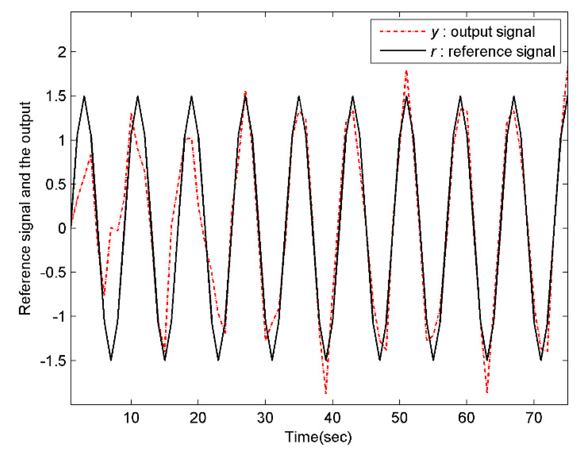
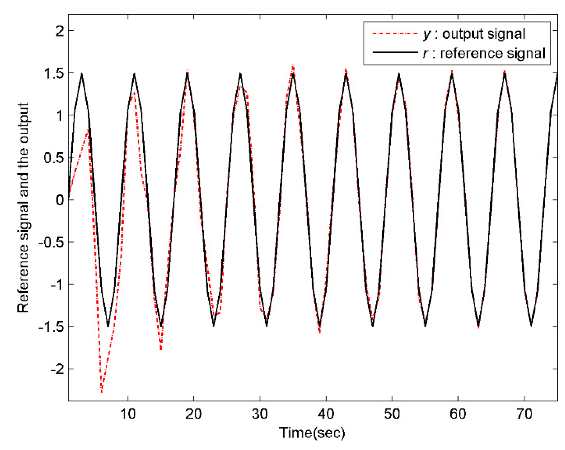
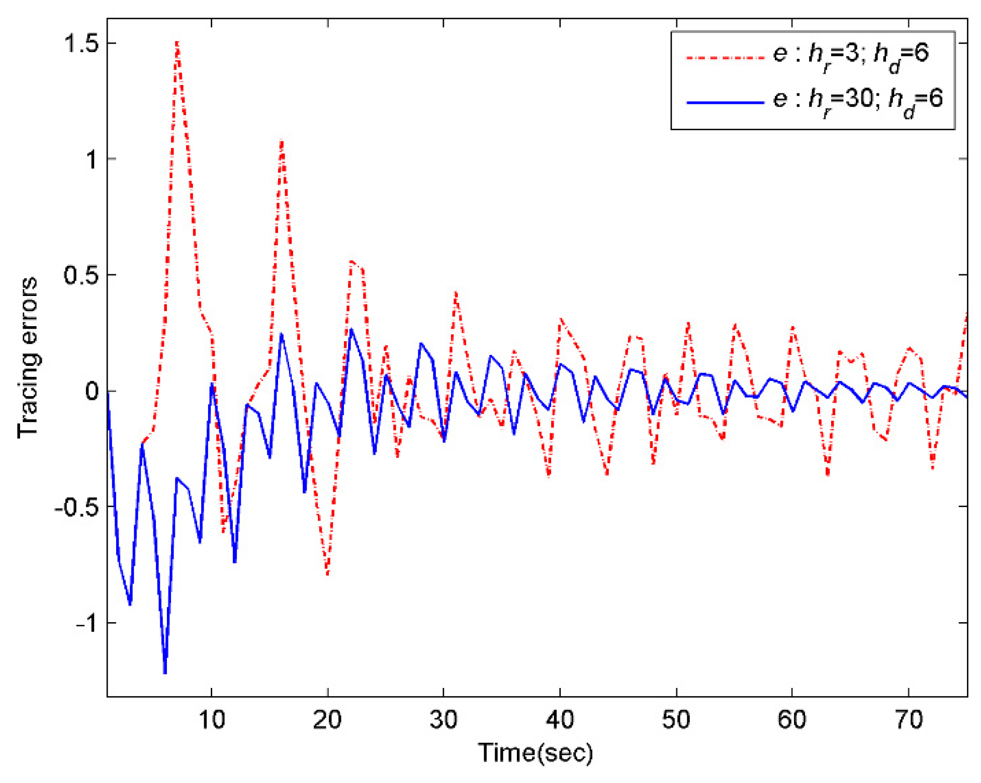
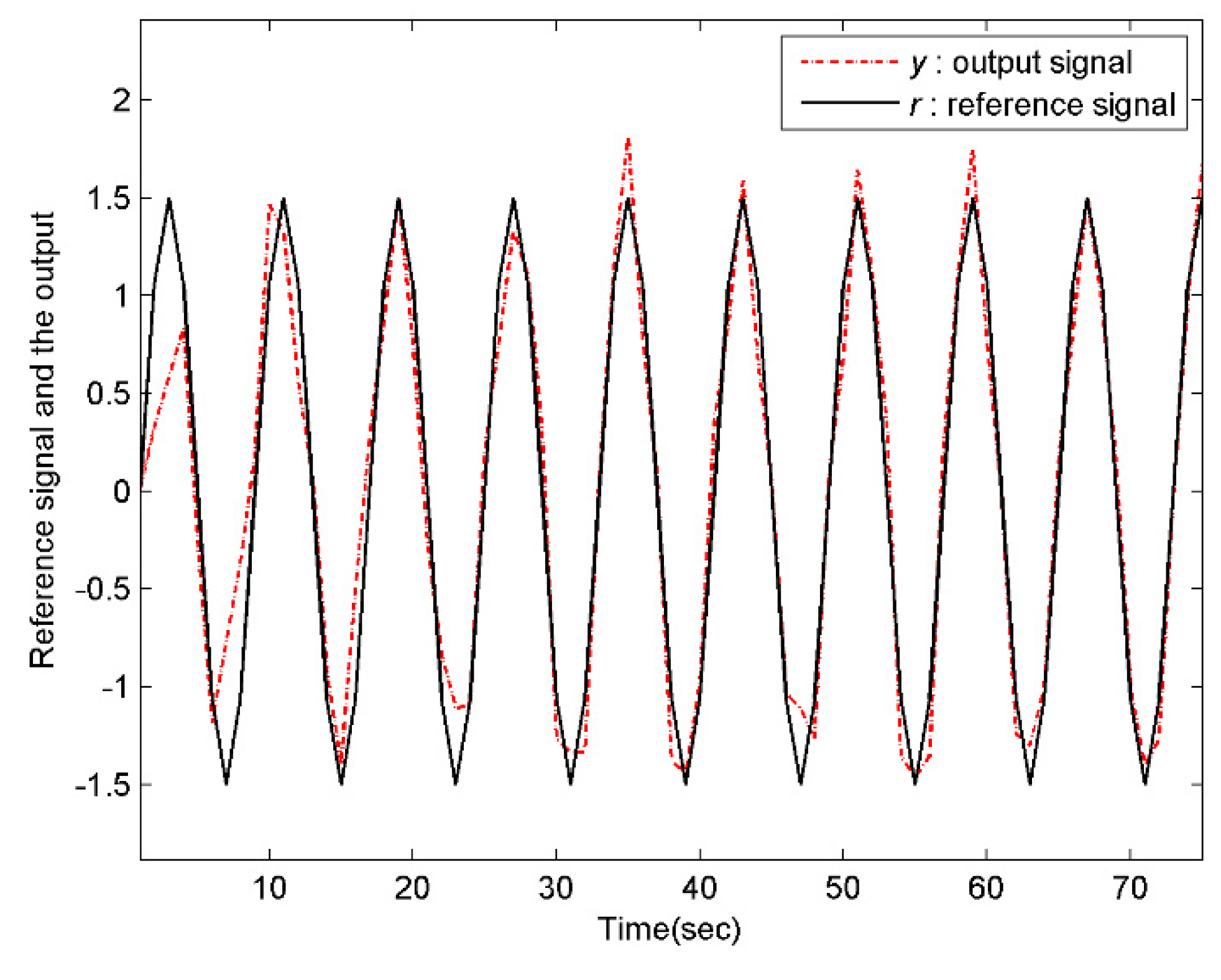
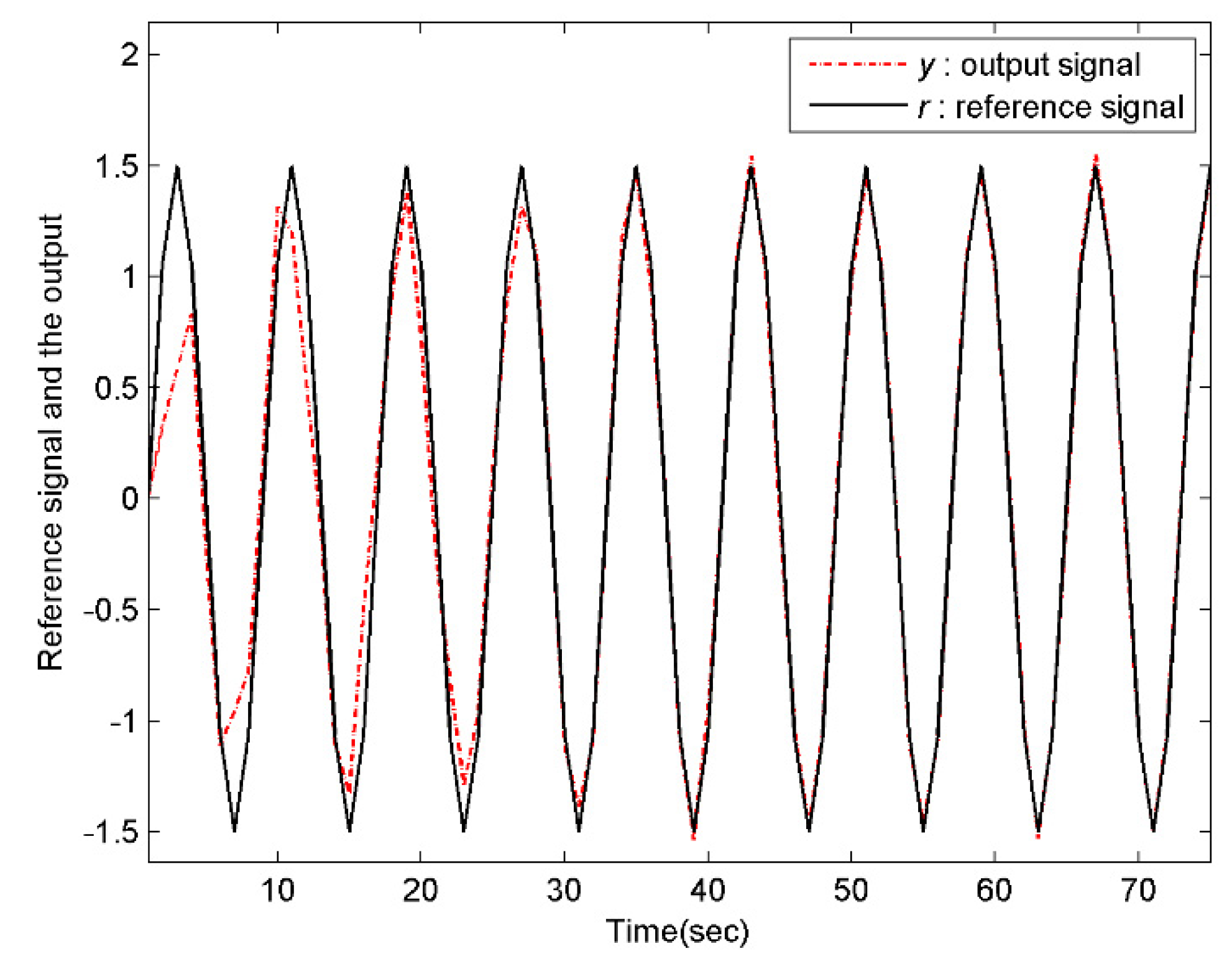
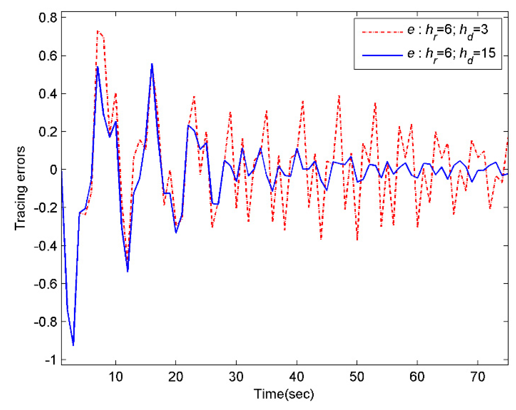
Assume that the both the reference signal and the disturbance signal are previewable. In order to reflect the influence of the preview information on tracking effectiveness, the numeric simulation will be conducted under the following four scenarios, i.e., $h_r=3$, $h_d=6$; $h_r=30$, $h_d=6$; $h_r=6$, $h_d=3$; $h_r=6$, $h_d=15$. Specifically, select the initial values $x_0={\left[\begin{array}{cc}0.01& 0.01\end{array}\right]}^T$ and $x_c={\left[\begin{array}{cccc}0& 0& 0& 0\end{array}\right]}^T$ for the system and the internal model compensator, respectively. Moreover, choose the weight matrices $Q_E=100\cdot I_3$, $Q_c=10\cdot I_4$ and $H=5000\cdot I_3$ for the performance index function (27). Then, according to the above discussions, the conditions of the Theorem 5 are all satisfied. As a result, the controller designed in this paper can drive the multirate system to complete the preview tracking. Using MATLAB to perform the simulation.

As what can be seen from Figure 1, Figure 2, Figure 3, Figure 4, Figure 5 and Figure 6, the larger the preview length, the better the tracking performance. That is, the controller (34) has advantage of overcoming the external disturbance in a shorter time and track the preview signal more accurately. Therefore, the controller (34) designed for the preview tracking problem is effective.

6. Conclusions

In this research, the preview tracking problem for discrete-time multirate systems was studied with external disturbance. Discrete lifting method and state augmentation technique, which together with internal model principle, were adopted to transform the original problem into the output regulation problem for a single-rate augmented system. This study is the development of preview control for discrete-time linear multirate systems [34] since the scenario of the unattenuated reference signal and disturbance signal was considered. Note that the state and output signals in this research were obtained by equal period sampling, in practical, since the bandwidth of network transmission is limited, quantized sampling is unavoidable. Future work will focus on considering the preview tracking control for discrete-time linear systems with input and output quantization.