Article

A Comparative Study of the Fractional-Order Clock Chemical Model

by
Hari Mohan Srivastava
1,2,3,* and
Khaled M. Saad
4,5
1
Department of Mathematics and Statistics, University of Victoria, Victoria, BC V8W 3R4, Canada
2
Department of Medical Research, China Medical University Hospital, China Medical University, Taichung 40204, Taiwan
3
Department of Mathematics and Informatics, Azerbaijan University, 71 Jeyhun Hajibeyli Street, Baku AZ1007, Azerbaijan
4
Department of Mathematics, College of Arts and Sciences, Najran University, Najran P.O. Box 1988, Saudi Arabia
5
Department of Mathematics, Faculty of Applied Science, Taiz University, Taiz P.O. Box 6803, Yemen
*
Author to whom correspondence should be addressed.
Mathematics 2020, 8(9), 1436; https://doi.org/10.3390/math8091436
Submission received: 3 August 2020 / Revised: 20 August 2020 / Accepted: 24 August 2020 / Published: 27 August 2020
(This article belongs to the Special Issue New Frontiers in Applied Mathematics and Statistics)

Abstract

:
In this paper, a comparative study has been made between different algorithms to find the numerical solutions of the fractional-order clock chemical model (FOCCM). The spectral collocation method (SCM) with the shifted Legendre polynomials, the two-stage fractional Runge–Kutta method (TSFRK) and the four-stage fractional Runge–Kutta method (FSFRK) are used to approximate the numerical solutions of FOCCM. Our results are compared with the results obtained for the numerical solutions that are based upon the fundamental theorem of fractional calculus as well as the Lagrange polynomial interpolation (LPI). Firstly, the accuracy of the results is checked by computing the absolute error between the numerical solutions by using SCM, TSFRK, FSFRK, and LPI and the exact solution in the case of the fractional-order logistic equation (FOLE). The numerical results demonstrate the accuracy of the proposed method. It is observed that the FSFRK is better than those by SCM, TSFRK and LPI in the case of an integer order. However, the non-integer orders in the cases of the SCM and LPI are better than those obtained by using the TSFRK and FSFRK. Secondly, the absolute error between the numerical solutions of FOCCM based upon SCM, TSFFRK, FSFRK, and LPI for integer order and non-integer order has been computed. The absolute error in the case of the integer order by using the three methods of the third order is considered. For the non-integer order, the order of the absolute error in the case of SCM is found to be the best. Finally, these results are graphically illustrated by means of different figures.

1. Introduction, Definitions and Preliminaries

During the past several decades, the classical calculus has been generalized into fractional calculus. The generalization was the result of a simple question that Leibniz asked in his letter to L’Hôpital about the derivative of order 1 2 . In recent years, many researchers have caught the attention of modeling real-world phenomena by using fractional-order derivatives. The dynamics of many applied problems has been modeled and studied using the concept of fractional-order derivatives. Such problems appear in, for example, biology and physics, ecology, engineering, and various other fields of applied sciences, and so on (see, for details, [1,2,3]; also see the recently-published survey-cum-expository review article [4]).
The main goal of our study in this work is to find the numerical solutions of the fractional-order clock chemical model, which is, we have presented a numerical study. In fact, most of the problems related to the real world are not solved exactly. Hence, in order to verify an appropriate numerical method to find the approximate solution of the fractional-order clock chemical model, a comparative study is conducted between a number of applicable numerical methods. This is indeed useful for many researchers who may use these methods in order to solve other systems and models. Moreover, the fractional-order clock chemical model provides an application of a real-world problem and we need to contribute toward finding its numerical solution, as followed by many researchers in this field. To the best our knowledge, this fractional model has not been studied numerically so far, except possibly in one of our recent papers (see [3]) and, of course, in this work. This justifies the importance of our contribution.
One of the features of mathematical modeling of various biological phenomena is that the mathematical model is represented as a mathematical function in time and the involved parameters. Hence, in this case, we can find the numerical solution to the model and also the parameters that affect this model can be appropriately controlled (see [5,6,7,8,9,10,11,12,13,14,15,16,17,18]).
In this paper, we first contribute toward studying the effect of changes in the order of the fractional derivatives involved. We verify the accuracy of the approximate solution in the presence of a complete solution to the fractional logistic growth model. We then employ different numerical methods in finding approximate solutions for the fractional-order clock chemical model. We also numerically analyze and graphically illustrate these results by means of different figures.
In this section, we give some basic definitions and properties of fractional calculus theory (see, for example [1,2]).
Definition 1.
For ν > 0 , the Liouville–Caputo fractional derivative of order ν , denoted by a + LC D ζ ν , is defined by
a + LC D ζ ν α ( ζ ) = 1 Γ ( n ν ) a + ζ ( ζ η ) n ν 1 D n α ( η ) d η ,
( n 1 < ν < n ; n N = { 1 , 2 , 3 , } ) ,
a + LC D ζ ν = D ν ( ν N ) ,
where D = d d ζ .
The problem under study here is the chemical clock reaction model which is given by [3]. We now replace the ordinary derivative in this model by a fractional-order derivative in the Liouville-Caputo sense (see Definition 1 above), which we have chosen to use here for simplicity instead of Definition 1. The fractional-order chemical clock reaction model is then given by
D ν α 1 ( ζ ) = μ e ε δ ζ α 1 ( ζ ) α 2 ( ζ ) ,
D ν α 2 ( ζ ) = α 1 ( ζ ) α 2 ( ζ ) α 2 ( ζ ) δ α 1 ( ζ ) + α 2 ( ζ ) μ ε δ 1 e ε δ ζ + λ 1 ,
α 3 ( ζ ) = α 1 ( ζ ) + α 2 ( ζ ) μ ε δ 1 e ε δ ζ + λ 1
and
α 1 ( 0 ) = 0 , α 2 ( 0 ) = 1 and α 3 ( 0 ) = λ , ζ 0 .
For more details about this model, one may see its mathematical formulation of in [19,20] to know the definitions for the chemical concentrations α 1 ( ζ ) , α 2 ( ζ ) and α 3 ( ζ ) and the parameters μ , ϵ , δ , and λ .
The main structure of this paper is as follows. In Section 2, the fractional-order Logistic equation and is exact solution are presented. In Section 3, the implementation the spectral collocation and simulation are given. In Section 4, the generalized Runge–Kutta methods are proposed. In Section 5, the numerical results and a systematic discussion are introduced. Finally, in Section 6, the conclusion is presented.

2. The Fractional-Order Logistic Equation

In this section, we introduce the fractional-order Logistic growth model and their exact solution for 0 < ν 1 . The dual aspects of complexity, fractional growth and nonlinearly-induced saturation emerge into the fractional-order logistic equation given by
D ν α ( ζ ) = K ν α ( ζ ) 1 α ( ζ ) α ( 0 ) = α 0 .
West [21] (see also [22]) constructed an exact solution to the FOLE by using the Carleman embedding technique. The exact solution of (6) is given by
α ( ζ ) = n = 0 α 0 1 α 0 n E ν ( n K ν ζ ν ) ,
where
E ν ( ζ ) = n = 0 ζ n Γ ( n ν + 1 )
is the Mittag–Leffler function.

3. The Spectral Collocation Method (SCM)

In this section, we apply the SCM for evaluating the numerical solutions of the (2)–(4). In many scientific applications, orthogonal functions and spectral methods have been used to find approximate solutions for fractional differential equations. Using these methods, we can transform the fractional differential equations into a set of algebraic equations. Subsequently, the algebraic equations are solved by one or the other of several known numerical methods (see [23,24,25]).
We begin by defining the shifted Legendre polynomials on the interval [ 0 , 1 ] with the variable z = 2 ζ 1 . These polynomials have the following property:
P s ( ζ ) = P s ( 2 ζ 1 ) = P 2 s ( ζ ) ,
where the set { P s ( z ) : s = 0 , 1 , 2 , } forms a family of orthogonal Legendre polynomials on the interval [ 1 , 1 ] (see, for details [26]).
The analytic form of the shifted Legendre polynomials of degree s is given by
P ˜ ( ζ ) = k = 0 s ( 1 ) s + k ( s + k ) ! ( k ! ) 2 ( s k ) ! ζ k ( P ˜ 0 ( ζ ) = 1 ; P ˜ 1 ( ζ ) = 2 ζ 1 ; s = 2 , 3 , 4 , ) .
The function α ( ζ ) L 2 [ 0 , 1 ] can be expressed and approximated as a linear combination of the first ( m + 1 ) terms of P ˜ s ( ζ ) , as follows:
α ( ζ ) α m ( ζ ) = i = 0 m a i P ˜ i ( ζ ) , m = 1 , 2 , 3 , 4 , .
where the coefficients a i are given by
a i = ( 2 i + 1 ) 0 1 α ( ζ ) P ˜ i ( ζ ) d ζ ( i = 0 , 1 , 2 , ) .
We now state the following useful theorem.
Theorem 1
([27]). Let α ( ζ ) be approximated by the shifted Legendre polynomials in (9). Suppose also that ν > 0 . Then
D ν α ( ζ ) = i = ν m k = ν i a i χ i k ( ν ) ζ k ν ,
where
χ i , k ( ν ) = ( i + k ) ! Γ ( k + 1 ) ( k ! ) 2 ( i k ) ! Γ ( k α + 1 ) .
We now implement the SCM for treating the given problem numerically and convert it into a non-linear system of algebraic equations. We will then solve the resulting system of algebraic equations using the Newton iteration method (see [28]).
In order to achieve this implementation of the SCM to solve numerically the suggested model given by (2)–(5), we approximate α 1 ( t ) , α 2 ( ζ ) and α 3 ( ζ ) by α 1 , m ( t ) , α 2 , m ( ζ ) and α 3 , m ( t ) , respectively, as follows:
α 1 , m ( ζ ) = k = 0 m a k P ˜ k ( ζ ) , α 2 , m ( ζ ) = k = 0 m b k P ˜ k ( ζ ) , and α 3 , m ( ζ ) = k = 0 m c k P ˜ k ( ζ ) .
The connection between the Equations (2)–(5), (10), and (11) leads us to the following consequences:
i = ν m k = ν i a k χ i , k ( ν ) ζ k ν = μ e ε δ ζ k = 0 m a k P ˜ k ( ζ ) k = 0 m b k P ˜ k ( ζ ) ,
i = ν m k = ν i a k χ i , k ( ν ) ζ k ν = k = 0 m a k P ˜ k ( ζ ) k = 0 m b k P ˜ k ( ζ ) 1 δ k = 0 m b k P ˜ k ( ζ ) · k = 0 m b k P ˜ k ( ζ ) + k = 0 m b k P ˜ k ( ζ ) μ ε δ 1 e ε δ ζ , + λ 1
and
k = 0 m c k P ˜ k ( ζ ) = k = 0 m a k P ˜ k ( ζ ) + k = 0 N b k P ˜ k ( ζ ) μ ε δ 1 e ε δ ζ + λ 1 .
Moreover, the collocation for the system given by (12)–(14) at m of the nodes ζ p , which is, the roots of P ˜ k ( ζ ) , yields
i = ν m k = ν i a k χ i , k ( ν ) ζ p k ν = μ e ε δ ζ p k = 0 m a k P ˜ k ( ζ p ) k = 0 m b k P ˜ k ( ζ p ) ,
i = ν m k = ν i b k χ i , k ( ν ) ζ p k ν = k = 0 m a k P ˜ k ( ζ p ) k = 0 N b k P ˜ k ( ζ p ) 1 δ k = 0 m b k P ˜ k ( ζ p ) · k = 0 m a k P ˜ k ( ζ p ) + k = 0 m b k P ˜ k ( ζ p ) μ ε δ 1 e ε δ ζ p , + λ 1
and
k = 0 m c k P ˜ k ( ζ p ) = k = 0 m a k P ˜ k ( ζ p ) + k = 0 m b k P ˜ k ( ζ p ) μ ε δ 1 e ε δ ζ p + λ 1 .
Now, upon substituting from Equation (11) into the initial conditions given by (5), we obtain the following three equations:
k = 0 m Δ k a k = 0 ,
k = 0 m Δ k b k = 1 ,
k = 0 m Δ k c k = λ ,
where
Δ k = P ˜ k ( 0 ) = ( 1 ) k ( 2 k + 1 ) ( k = 0 , 1 , , m ) .
Equations (15)–(17), together with the three equations in (18), provide a system of 3 ( m + 1 ) algebraic equations. The involved unknowns a k , b k , c k ( k = 0 , 1 , , m ) will be obtained by solving the system given by (15)–(18) with the help of the Newton iteration method.

4. Runge-Kutta Methods

In this section, we apply the fractional Runge–Kutta method of order 2 and of order 4, which was used in [29,30], respectively. To this end, we construct the schemes for fractional model given by (2)–(4) with these algorithms.

4.1. Two-Stage Fractional Runge-Kutta Method

The numerical solutions of Equations (2)–(4), which are based on TSFRK, are given by
α 1 ( ζ n + 1 ) = α 1 ( ζ n ) + h ν 2 Γ ( 1 + ν ) ( K 2 , 1 + K 2 , 2 ) ,
α 2 ( ζ n + 1 ) = α 2 ( ζ n ) + h ν 2 Γ ( 1 + ν ) ( M 2 , 1 + M 2 , 2 ) ,
α 3 ( ζ n + 1 ) = α 1 ( ζ n ) + α 2 ( ζ n ) μ ε δ 1 e ε δ ζ n + λ 1 ,
where
K 2 , 1 = f ζ n , α 1 ( ζ n ) , α 2 ( ζ n ) ,
M 2 , 1 = g ζ n , α 1 ( ζ n ) , α 2 ( ζ n ) ,
K 2 , 2 = f ( ζ n + 2 Γ ( 1 + ν ) Γ ( 1 + 2 ν ) h ν , α 1 ( ζ n ) + 2 Γ ( 1 + ν ) Γ ( 1 + 2 ν ) h ν K 2 , 1 , α 2 ( ζ n ) + 2 Γ ( 1 + ν ) Γ ( 1 + 2 ν ) h ν M 2 , 1 ) ,
M 2 , 2 = g ( ζ n + 2 Γ ( 1 + ν ) Γ ( 1 + 2 ν ) h ν , α 1 ( ζ n ) + 2 Γ ( 1 + ν ) Γ ( 1 + 2 ν ) h ν K 2 , 1 , α 2 ( ζ n ) + 2 Γ ( 1 + ν ) Γ ( 1 + 2 ν ) h ν M 2 , 1 ) ,
f ζ , α 1 ( ζ ) , α 2 ( ζ ) = μ e ε δ ζ α 1 ( ζ ) α 2 ( ζ )
and
g ζ , α 1 ( ζ ) , α 2 ( ζ ) = α 1 ( ζ ) α 2 ( ζ ) α 2 ( ζ ) δ α 1 ( ζ ) + α 2 ( ζ ) μ ε δ 1 e ε δ ζ + λ 1 .
For further details about the derivation of this algorithm, see [29].

4.2. Four-Stage Fractional Runge-Kutta

In this subsection, we employ the algorithm that was derived in [30] on the fractional model given by (2)–(4), as in the above section with TSFRK, such that
α 1 ( ζ n + 1 ) = α 1 ( ζ n ) + 1 6 ( K 4 , 1 + 2 K 4 , 2 + 2 K 4 , 3 + K 4 , 4 ) ,
α 2 ( ζ n + 1 ) = α 2 ( ζ n ) + 1 6 ( M 4 , 1 + 2 M 4 , 2 + 2 M 4 , 3 + M 4 , 4 )
and
α 3 ( ζ n + 1 ) = α 1 ( ζ n ) + α 2 ( ζ n ) μ ε δ 1 e ε δ ζ n + λ 1 ,
where
K 4 , 1 = h ν Γ ( 1 + ν ) f ζ n , α 1 ( ζ n ) , α 2 ( ζ n ) ) ,
M 4 , 1 = h ν Γ ( 1 + ν ) g ζ n , α 1 ( ζ n ) , α 2 ( ζ n ) ,
K 4 , 2 = h ν Γ ( 1 + ν ) f ζ n + h ν 2 Γ ( 1 + ν ) , α 1 ( ζ n ) + 1 2 K 4 , 1 , α 2 ( ζ n ) + 1 2 M 4 , 1 ,
M 4 , 2 = h ν Γ ( 1 + ν ) g ζ n + h ν 2 Γ ( 1 + ν ) , α 1 ( ζ n ) + 1 2 K 4 , 1 , α 2 ( ζ n ) + 1 2 M 4 , 1 ,
K 4 , 3 = h ν Γ ( 1 + ν ) f ζ n + h ν 2 Γ ( 1 + ν ) , α 1 ( ζ n ) + 1 2 , K 4 , 2 , α 2 ( ζ n ) + 1 2 M 4 , 2 ,
M 4 , 3 = h ν Γ ( 1 + ν ) g ζ n + h ν 2 Γ ( 1 + ν ) , α 1 ( ζ n ) + 1 2 K 4 , 2 , α 2 ( ζ n ) + 1 2 M 4 , 2 ,
K 4 , 4 = h ν Γ ( 1 + ν ) f ζ n + h ν Γ ( 1 + ν ) , α 1 ( ζ n ) + K 4 , 3 , α 2 ( ζ n ) + M 4 , 3
and
M 4 , 4 = h ν Γ ( 1 + ν ) g ζ n + h ν Γ ( 1 + ν ) , α 1 ( ζ n ) + K 4 , 3 , α 2 ( ζ n ) + M 4 , 3 .
For further details on the four-stage fractional Runge–Kutta (FSFRK) method, see [30].

5. Numerical Results and Discussion

In this section, we investigate the numerical solutions of the fractional-order chemical clock reaction model by implementing the SCM, TSFRK, FSFRK, methods. We then compare the obtained results with these methods with the results of Lagrange polynomial interpolation (LPI) in [3]. We first conduct a test for all methods on fractional-order Logistic equation, which has an exact solution for integer as well as non-integer order. Figure 1a–d graphically illustrate the absolute error between the exact solution of FOLE and the corresponding numerical solutions by SCM, TSFRK, FSFRK, and LPI, respectively, for ν = 1 , α ( 0 ) = 0.75 , h = 0.03 , m = 21 and K = 1 . In these figures, we notice that the absolute error based upon the FSFRK are much better than those of the SCM, the TSFRK, and the LPI methods when the order of logistic equation is 1. In this case, the order of the error for FSFRK is 10 14 . In Figure 2a–d, we evaluate the absolute error for non-integer order of FOLE between the exact solution of FOLE and SCM, TSFRK, FSFRK, and LPI, respectively. In this case, we set ν = 0.9 , α ( 0 ) = 0.75 , h = 0.03 , m = 21 and K = 1 . In these figures, the orders of the SCM and the LPI are better than those of the TSFRK and FSFRK. The order of error for the SCM and the LPI is 10 2 , whereas, in the case of the TSFRK and the FSFRK, is 10 1 . Accordingly, based on this investigation, we can take the LPI [3] as a method to compare our numerical solution of the fractional-order clock chemical model based on the SCM, TSFRK and FSFRK. Additionally, we investigate in details the error in Table 1 and Table 2. Table 1 and Table 2 represent the absolute error between the SCM, the TSFR, the FSFRK, and the LPI methods, respectively, with the exact solution of fractional-order logistic equation. In these table, the effect of the changing of the order of the differential equation from the integer order to the non-integer order is the most important parameter in this work. This, in fact, is the aim of this work. The effect of the parameter K is also studied. The time and parameters h and m are fixed. Through Table 1 and Table 2, we make the following observations:
  • In Table 1, we notice that the order of the errors are small in all of the methods used here. Additionally, in the cases of the SCM and the FSFRK methods are much better than those in the cases of the TSFR and the LPI methods.
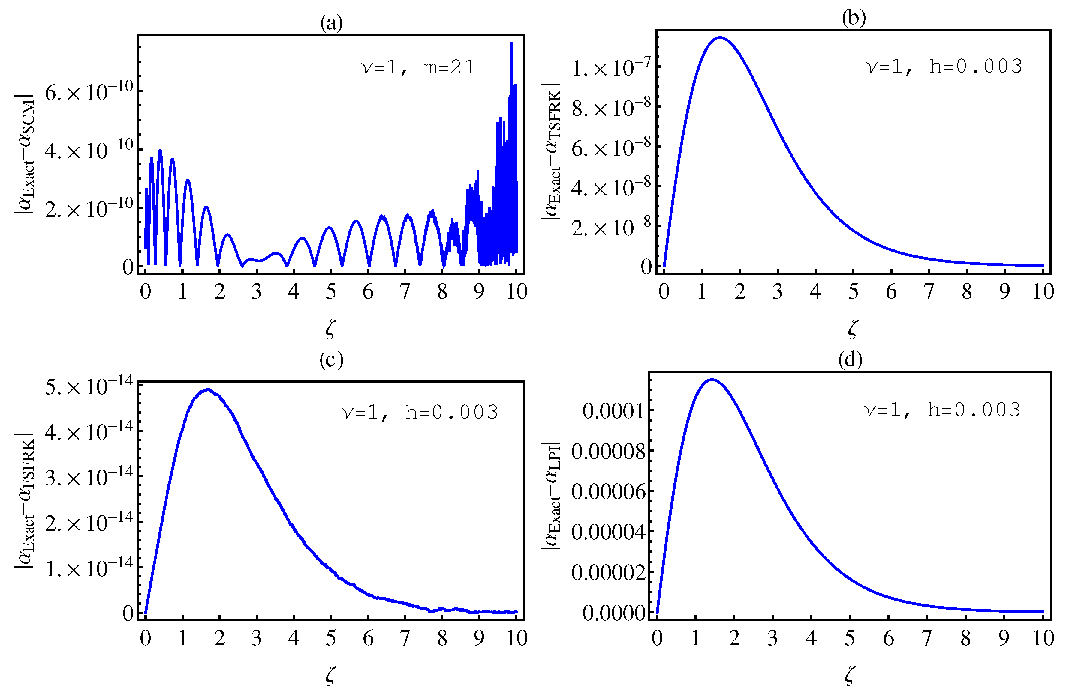
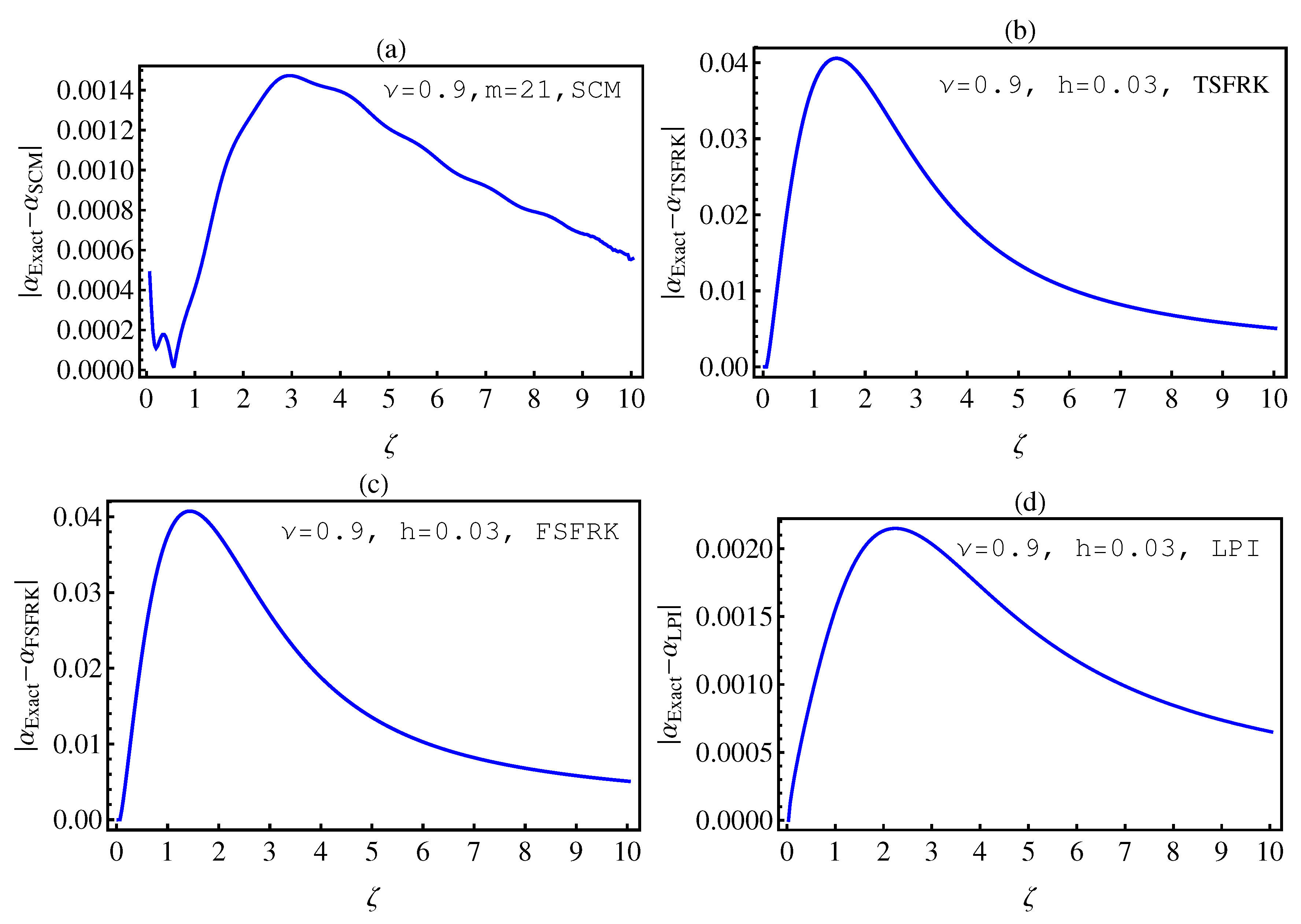
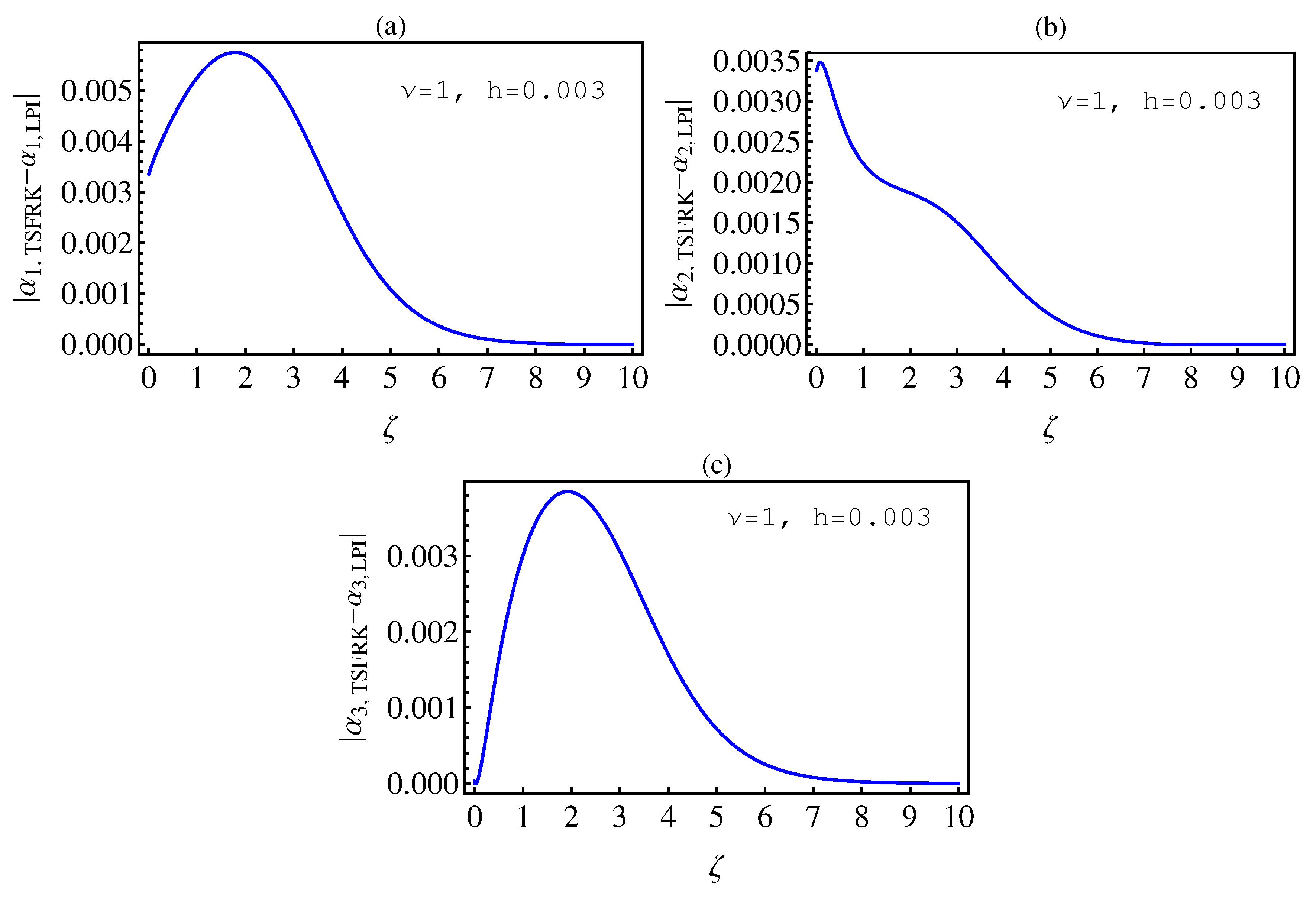
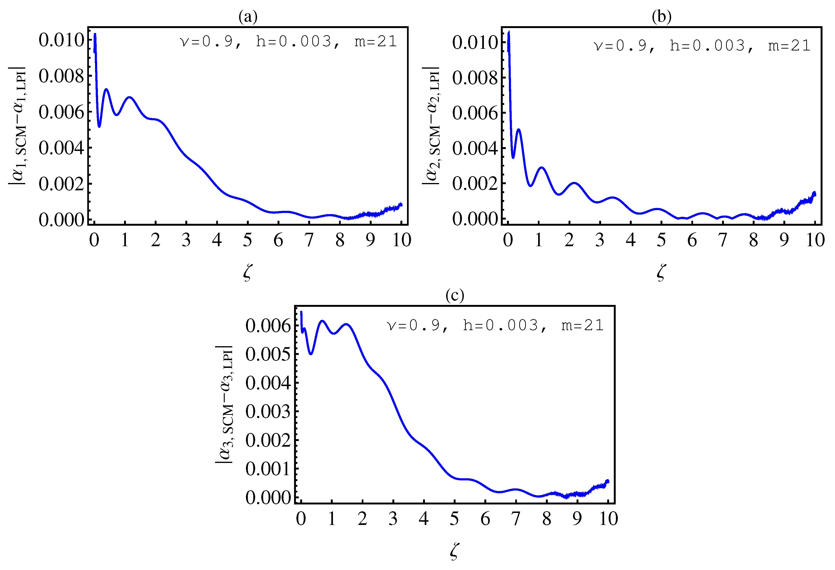
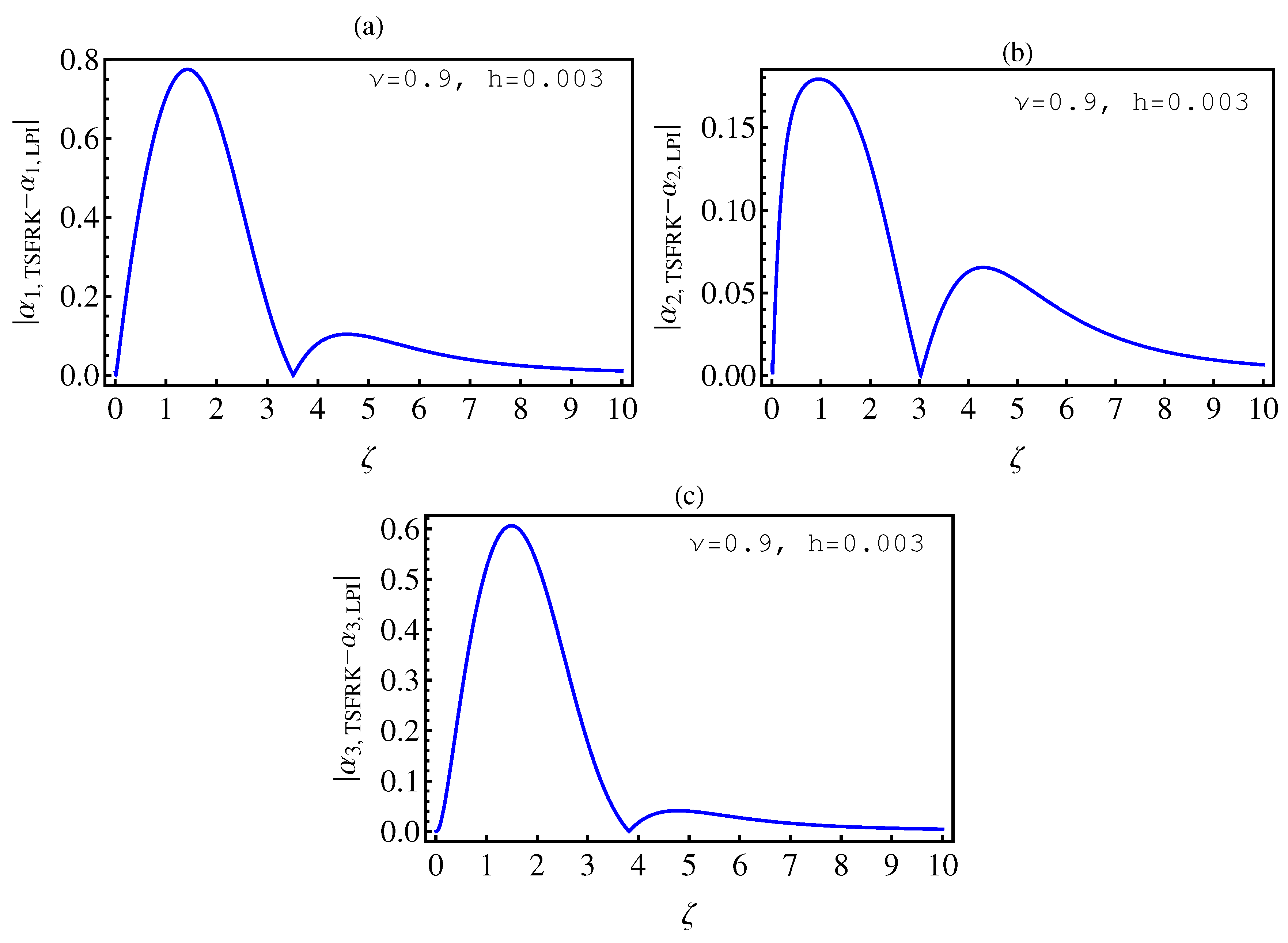
  • In Table 2, we see that the orders of the errors for all of the methods are close to each other. However, the SCM and LPI methods are better than the TSFRK and FSFRK methods. Therefore, we cannot say here that one of the methods is the best absolutely, but we can say that some of the methods are better than the other methods. In Figure 3, Figure 4 and Figure 5, we compute the absolute error between LPI and SCM, TSFRK, and FSFRK, respectively. In these figures, we set ν = 1 , h = 0.03 , m = 21 , λ = 2 , ϵ = 1 , μ = 2 , δ = 1 and the initial values are set as α 1 ( 0 ) = 0 , α 2 ( 0 ) = 1 and α 3 ( 0 ) = λ . From these figures, we observe that the order of the error for the SCM, TSFRK, and FSFRK methods is 10 3 . In Figure 6, Figure 7 and Figure 8, we find the absolute error for the same caption as those of Figure 3, Figure 4 and Figure 5, but with ν = 0.9 . In the non-integer order, we have obtained the same results, as illustrated in Figure 2. The order of the error of the SCM is better than those of the TSFRK and FSFRK. From this investigation, we can say that the numerical solutions based upon the SCM and LPI methods are remarkably accurate and effective in the case of non-integer order.

6.  Conclusions

In this paper, we have presented three algorithms to find the numerical solutions of the chemical clock model. We applied each of these algorithms to the fractional-order chemical clock reaction model. In order to verify the efficiency of the results, which we have investigated in this paper, we introduced the fractional-order logistic equation with its exact solution. We compared the numerical solutions based on the SCM, TSFRK, FSFRK, and LPI, respectively, with the exact solution of the fractional-order logistic equation for integer and non integer orders. We have noted that the error for all of the methods were very small. However, the SCM and the FSFRK are better than TSFRK and LPI when the order of the logistic equation was an integer. But, if the order is non-integer, the SCM and LPI are better than the TSFRK and FSFRK. The order of error here, as is evident from the figures and the Tables, with respect to SCM and LPI is 10 2 . In the case of the TSFRK and FSFRK, the order of error is found to be 10 1 . For the fractional-order chemical clock reaction model, we have also compared the results with the corresponding previously-published results for integer order and non-integer order. We have thereby noticed that the error in the case of integer order for SCM, TSFRK and FSFRK are small for all methods. However, for the case of non-integer order, the SCM is remarkably better than the TSFRK and FSFRK. Finally, in this paper, we presented an analytical comparative study between four methods to find the numerical solutions to fractional differential equations, and the accuracy of the Runge-Kutta methods as compared to other methods was studied. As for the Runge-Kutta methods of finding numerical solutions to fractional differential equations, they are still new. Additionally, as far as we know, there are only two or three studies in this direction. Therefore, in our next work, we will use these methods to find and study the behavior of the numerical solutions for systems of fractional differential equations. The various results, which we have presented in this paper, have indeed been numerically analyzed and graphically illustrated by means of different figures and tables.

Author Contributions

H.M.S. suggested and initiated this work, performed its validation, as well as reviewed and edited the paper. K.M.S. performed the formal analysis of the investigation, the methodology, the software, and wrote the first draft of the paper. All authors have read and agreed to the published version of the manuscript.

Funding

This research received no external funding.

Conflicts of Interest

The authors declare that they have no conflict of interest.

References

  1. Podlubny, I. Fractional Differential Equations: An Introduction to Fractional Derivatives, Fractional Differential Equations, to Methods of Their Solution and Some of Their Applications; Mathematics in Science and Engineering; Academic Press: New York, NY, USA; London, UK; Sydney, Australia; Tokyo, Japan; Toronto, ON, Canada, 1999; Volume 198. [Google Scholar]
  2. Kilbas, A.A.; Srivastava, H.M.; Trujillo, J.J. Theory and Applications of Fractional Differential Equations; North-Holland Mathematical Studies; Elsevier (North-Holland) Science Publishers: Amsterdam, The Netherlands; London, UK; New York, NY, USA, 2006; Volume 204. [Google Scholar]
  3. Saad, K.M.; Srivastava, H.M.; Gómez-Aguilar, J.F. A fractional quadratic autocatalysis associated with chemical clock reactions involving linear inhibition. Chaos Solitons Fract. 2020, 132, 1–9. [Google Scholar] [CrossRef]
  4. Srivastava, H.M. Fractional-order derivatives and integrals: Introductory overview and recent developments. Kyungpook Math. J. 2020, 60, 73–116. [Google Scholar]
  5. Khader, M.M.; Saad, K.M. Numerical treatment for studying the blood ethanol concentration systems with different forms of fractional derivatives. Int. J. Mod. Phys. C 2020, 31, 1–13. [Google Scholar] [CrossRef]
  6. Abdo, M.S.; Shah, K.; Wahash, H.A.; Panchal, S.K. On a comprehensive model of the novel corona-virus (COVID-19) under Mittag-Leffler derivative. Chaos Solitons Fract. 2020, 135, 109867. [Google Scholar] [CrossRef]
  7. Srivastava, H.M.; Saad, K.M.; Gómez-Aguilar, J.F.; Almadiy, A.A. Some new mathematical models of the fractional-order system of human immune against IAV infection. Math. Biosci. Engrg. 2020, 17, 4942–4969. [Google Scholar] [CrossRef]
  8. Srivastava, H.M.; Saad, K.M. New approximate solution of the time-fractional Nagumo equation involving fractional integrals without singular kernel. Appl. Math. Inform. Sci. 2020, 14, 1–8. [Google Scholar]
  9. Ghanbari, B.; Günerhan, H.; Srivastava, H.M. An application of the Atangana-Baleanu fractional derivative in mathematical biology: A three-species predator-prey model. Chaos Solitons Fract. 2020, 138, 109919. [Google Scholar] [CrossRef]
  10. Srivastava, H.M.; Jena, R.M.; Chakraverty, S.; Jena, S.K. Dynamic response analysis of fractionally-damped generalized Bagley-Torvik equation subject to external loads. Russ. J. Math. Phys. 2020, 27, 254–268. [Google Scholar] [CrossRef]
  11. Area, I.; Ndairou, F.; Nieto, J.J.; Silva, C.J. Ebola model and optimal control with vaccination constraints. J. Ind. Manag. Optim. 2018, 14, 427–446. [Google Scholar] [CrossRef] [Green Version]
  12. Srivastava, H.M.; Dubey, R.S.; Jain, M. A study of the fractional-order mathematical model of diabetes and its resulting complications. Math. Methods Appl. Sci. 2019, 42, 4570–4583. [Google Scholar] [CrossRef]
  13. Srivastava, H.M.; Günerhan, H. Analytical and approximate solutions of fractional-order susceptible-infected-recovered epidemic model of childhood disease. Math. Methods Appl. Sci. 2019, 42, 935–941. [Google Scholar] [CrossRef]
  14. Baleanu, D.; Jajarmi, A.; Mohammad, H.; Rezapour, S. A new study on the mathematical modelling of human liver with Caputo-Fabrizio fractional derivative. Chaos Solitons Fract. 2020, 134, 1–13. [Google Scholar] [CrossRef]
  15. Saad, K.M.; Al-Sharif, E.H.F. Comparative study of a cubic autocatalytic reaction via different analysis methods. Discret. Contin. Dyn. Syst. Ser. S 2019, 12, 665–684. [Google Scholar]
  16. Singh, H.; Pandey, R.K.; Srivastava, H.M. Solving non-linear fractional variational problems using Jacobi polynomials. Mathematics 2019, 7, 224. [Google Scholar] [CrossRef] [Green Version]
  17. Khader, M.M.; Saad, K.M. A numerical study using Chebyshev collocation method for a problem of biological invasion: Fractional Fisher equation. Int. J. Biomath. 2018, 11, 1–15. [Google Scholar] [CrossRef]
  18. Saad, K.M. New fractional derivative with non-singular kernel for deriving Legendre spectral collocation method. Alex. Eng. J. 2019, 59, 1909–1917. [Google Scholar] [CrossRef]
  19. Preece, S.J.; Billingham, J.; King, A.C. Chemical clock reactions: The effect of precursor consumption. J. Math. Chem. 1999, 26, 47–73. [Google Scholar] [CrossRef]
  20. Billingham, J.; Needham, D.J. Mathematical-modeling of chemical clock reactions II. A class of autocatalytic clock reaction schemes. J. Eng. Math. 1993, 27, 113–145. [Google Scholar] [CrossRef]
  21. West, B.J. Exact solution to fractional logistic equation. Phys. A Stat. Mech. Appl. 2015, 429, 103–108. [Google Scholar] [CrossRef]
  22. Carleman, T. Application de la théorie des équations intégrales linéaires aux systmes d’équations différentielles non linéaires. Phys. A Stat. Mech. Appl. 1932, 59, 63–87. [Google Scholar]
  23. Khalil, H.; Khan, R.A.; Al-Smadi, M.H.; Freihat, A.A.; Shawagfeh, N. New Operational matrix for shifted Legendre polynomials and fractional differential equations with variable coefficients. Punjab Univ. J. Math. 2015, 47, 1–23. [Google Scholar]
  24. Mohammadi, F.; Cattani, C. A generalized fractional-order Legendre wavelet Tau method for solving fractional differential equations. J. Comput. Appl. Math. 2018, 339, 306–316. [Google Scholar] [CrossRef]
  25. Mohammadi, F.; Mohyud-Din, S.T. A fractional-order Legendre collocation method for solving the Bagley-Torvik equations. Punjab Univ. J. Math. 2016, 269, 2–14. [Google Scholar] [CrossRef] [Green Version]
  26. Lebedev, N.N. Special Functions and Their Applications; Silverman, R.A., Translator; Dover Publications: New York, NY, USA, 1972; pp. 43–60. [Google Scholar]
  27. Khader, M.M.; Hendy, A.S. The approximate and exact solutions of the fractional-order delay differential equations using Legendre pseudo-spectral method. Int. J. Pure Appl. Math. 2012, 74, 287–297. [Google Scholar]
  28. Lubich, C. Discretized fractional calculus. SIAM J. Math. Anal. 1986, 17, 704–719. [Google Scholar] [CrossRef]
  29. Arshad, M.S.; Baleanu, D.; Riaz, M.B.; Abbas, M. A novel 2-stage fractional Runge-Kutta method for a time fractional logistic growth model. Discrete Dyn. Nat. Soc. 2020, 2020, 1020472. [Google Scholar] [CrossRef]
  30. Milici, C.; Machado, J.A.T.; Drăgănescu, G. Application of the Euler and Runge-Kutta generalized methods for FDE and symbolic packages in the analysis of some fractional attractors. Int. J. Nonlinear Sci. Numer. Simul. 2020, 21, 159–170. [Google Scholar] [CrossRef]
Figure 1. The absolute error between the exact and the numerical solutions of (6) based upon SCM (a); TSFRK (b); FSFRK (c) and LPI (d), respectively, for ν = 1.0 , h = 0.03 , m = 21 , K = 1.0 , α ( 0 ) = 0.75 .
Mathematics 08 01436 g001
Figure 2. The absolute error between the exact and the numerical solutions of (6) based upon SCM (a); TSFRK (b); FSFRK (c) and LPI (d), respectively, for ν = 0.9 , h = 0.03 , m = 21 , K = 1.0 , α ( 0 ) = 0.75 .
Mathematics 08 01436 g002
Figure 3. The absolute error between the numerical solutions of (2) to (4) based upon the LPI and the SCM for ν = 1 , h = 0.03 , m = 21 , λ = 2 , ϵ = 1 , μ = 2 , δ = 1 for the initial values α 1 ( 0 ) = 0 , α 2 ( 0 ) = 1 and α 3 ( 0 ) = λ ((a), (b) and (c), respectively).
Mathematics 08 01436 g003
Figure 4. The absolute error between the numerical solutions of (2) to (4) based upon the LPI and the TSFRK for ν = 1 , h = 0.03 , m = 21 , λ = 2 , ϵ = 1 , μ = 2 , δ = 1 and for the initial values α 1 ( 0 ) = 0 , α 2 ( 0 ) = 1 and α 3 ( 0 ) = λ ((a), (b) and (c), respectively).
Mathematics 08 01436 g004
Figure 5. The absolute error between the numerical solutions of (2) to (4) based upon: the LPI and the FSFRK for ν = 1 , h = 0.03 , m = 21 , λ = 2 , ϵ = 1 , μ = 2 , δ = 1 and for the initial values α 1 ( 0 ) = 0 , α 2 ( 0 ) = 1 and α 3 ( 0 ) = λ ((a), (b) and (c), respectively).
Mathematics 08 01436 g005
Figure 6. The absolute error between the numerical solutions of (2) to (4) based upon the LPI and the SCM for ν = 0.9 , h = 0.03 , m = 21 , λ = 2 , ϵ = 1 , μ = 2 , δ = 1 and for the initial values α 1 ( 0 ) = 0 , α 2 ( 0 ) = 1 and α 3 ( 0 ) = λ ((a), (b) and (c), respectively).
Mathematics 08 01436 g006
Figure 7. The absolute error between the numerical solutions of (2) to (4) based upon the LPI and the TSFRK for ν = 0.9 , h = 0.03 , m = 21 , λ = 2 , ϵ = 1 , μ = 2 , δ = 1 and for the initial values α 1 ( 0 ) = 0 , α 2 ( 0 ) = 1 and α 3 ( 0 ) = λ ((a), (b) and (c), respectively).
Mathematics 08 01436 g007
Figure 8. The absolute error between the numerical solutions of (2) to (4) based upon the LPI and the FSFRK for ν = 0.9 , h = 0.03 , m = 21 , λ = 2 , ϵ = 1 , μ = 2 , δ = 1 and for the initial values α 1 ( 0 ) = 0 , α 2 ( 0 ) = 1 and α 3 ( 0 ) = λ ((a), (b) and (c), respectively).
Mathematics 08 01436 g008
Table 1. The absolute error between the exact solution (6) and the numerical solutions by spectral collocation method (SCM), two-stage fractional Runge–Kutta (TSFR), four-stage fractional Runge–Kutta (FSFRK), and Lagrange polynomial interpolation (LPI), respectively, for  ν = 1 , ζ = 5 , h = 0.003 , m = 21 with different values of K.
K | Exact SCM | | Exact TSFRK | | Exact FSFRK | | Exact LPI |
0.2 1.53945 × 10 17 4.16541 × 10 9 3.33067 × 10 16 2.127988 × 10 5
0.4 6.72001 × 10 15 1.68964 × 10 8 1.88738 × 10 15 4.166692 × 10 5
0.6 6.696420 × 10 13 2.464570 × 10 8 3.663735 × 10 15 3.946389 × 10 5
0.8 6.34949 × 10 11 2.3406 × 10 8 7.43849 × 10 15 2.762099 × 10 5
1.0 1.281608 × 10 10 1.766755 × 10 8 9.325873 × 10 15 1.647932 × 10 5
Table 2. The absolute error between the exact solution (6) and the numerical solutions by SCM, TSFR, FSFRK, and LPI, respectively, for  ν = 0.8 , ζ = 5 , h = 0.003 , m = 21 with different values of K.
K | Exact SCM | | Exact TSFRK | | Exact FSFRK | | Exact LPI |
0.2 1.126692 × 10 3 1.08085 × 10 1 1.080896 × 10 1 1.184387 × 10 3
0.4 2.186600 × 10 3 6.576224 × 10 2 6.576269 × 10 2 2.257930 × 10 3
0.6 2.480864 × 10 3 4.453745 × 10 2 4.453749 × 10 2 2.553845 × 10 3
0.8 2.413834 × 10 3 3.293829 × 10 2 3.293830 × 10 2 2.486642 × 10 3
1.0 2.227433 × 10 3 2.591927 × 10 2 2.591927 × 10 2 2.301093 × 10 3

