Reconfigurable 3D CAD Feature Recognition Supporting Confluent n-Dimensional Topologies and Geometric Filters for Prismatic and Curved Models

Abstract

Feature Recognition (FR) in Computer-aided Design (CAD) models is central for Design and Manufacturing. FR is a problem whose computational burden is intractable (NP-hard), given that its underlying task is the detection of graph isomorphism. Until now, compromises have been reached by only using FACE-based geometric information of prismatic CAD models to prune the search domain. Responding to such shortcomings, this manuscript presents an interactive FR method that more aggressively prunes the search space with reconfigurable geometric tests. Unlike previous approaches, our reconfigurable FR addresses curved EDGEs and FACEs. This reconfigurable approach allows enforcing arbitrary confluent topologic and geometric filters, thus handling an expanded scope. The test sequence is itself a graph (i.e., not a linear or total-order sequence). Unlike the existing methods that are FACE-based, the present one permits combinations of topologies whose dimensions are two (SHELL or FACE), one (LOOP or EDGE), or 0 (VERTEX). This system has been implemented in an industrial environment, using icon graphs for the interactive rule configuration. The industrial instancing allows industry based customization and itis faster when compared to topology-based feature recognition. Future work is required in improving the robustness of search conditions, treating the problem of interacting or nested features, and improving the graphic input interface.

1. Introduction

Computer-aided Process Planning (CAPP) refers to the use of computational tools to automate and optimize the manufacturing planning process of an industrial product. To automatically determine the manufacturing techniques to be used in a certain product, it becomes necessary to be able to efficiently extract geometric features from the standarized version of the Computer-aided Design (CAD) model, a process known as “Automated Feature Recognition”.

An essential part in the efforts in CAD-CAPP systems research is the development of efficient and effective automated feature recognition algorithms. Features can describe form (form features), tolerances and finishing (precision features) or material treatment, and grade and properties (manufacturing features). Feature recognition algorithms focus on successfully identifying a region of a part with some interesting geometric or topological properties (form features). Precision and manufacturing features are out of the scope of such algorithms. Given that feature recognition is a problem whose computational burden is intractable (NP-hard) [1], geometric information from the CAD-based part model is used to prune the search space.

A number of feature recognition algorithms have been successfully implemented on boolean combinations of prismatic shapes, but most of the current algorithms fail to treat curved geometries and interacting features. This manuscript presents an extension of the reconfigurable feature recognition method introduced in [2] to allow for the treatment of different curved geometries using curvature-based filters. We also show an industry-based implementation (including its interactive graphic user interface) and the recognition process results.

In this manuscript, Section 1 introduces the industrial relevance of the problem and reviews the available relevant literature, highlighting the advantages and disadvantages of the existing methods of Feature Recognition. Section 2 presents and discusses the Methodology implemented, including the performance comparison with respect to other methods and the industrial instancing. Section 3 presents the results of the industrial implementation. Section 4 concludes the manuscript and discusses possible future developments.

1.1. Industrial Relevance

CAD three-dimensional (3D) Models are nowadays ubiquitous in many engineering contexts: in the automotive industry, for instance, more than 30.000 different parts are needed for complete vehicle, and most of them have a 3D CAD representation. These CAD models are created in different software packages (such as CATIA, SolidEdge, etc.) and by many companies working together (Tier-1 and Tier-2 system and component providers, Car OEM manufacturers, etc.). These CAD software packages have internal powerful tools to work in design, change, inspection, and assembly tasks, but in collaborative work using CAD models from different CAD systems, a standard 3D CAD Model representation is needed. For this, the STEP (ISO 10303-21 [3]) and the IGES standards [4] are widely used, not only to accomplish the transfer of models between CAD systems, but also to provide a vendor-independent 3D CAD model representation that can be used by any software tool.

In this sense, the ability to inspect the topology and the geometry of a standard 3D CAD representation model (such as STEP) is of high importance. More particularly, feature recognition is a task where this model inspection is relevant for engineers and designers, since they can easily find features of interest that are related with specific tasks: optimization, planning of additional manufacturing processes, detection of design errors, etc. However, the way to specify a feature recognition strategy is not evident, since it involves not only a geometry or topology intrinsic characteristics, but often also a meaning (a semantic level) [5], which is related to the application need. Several approaches for feature recognition have been proposed in the literature (as discussed in the literature review). Our approach allows the user to define reconfigurable arbitrary confluent tests with topologic and geometric filters, configured in a directed acyclic graph, thus offering the flexibility to define simple sequences or chains, but also more complex logic tests to be performed.

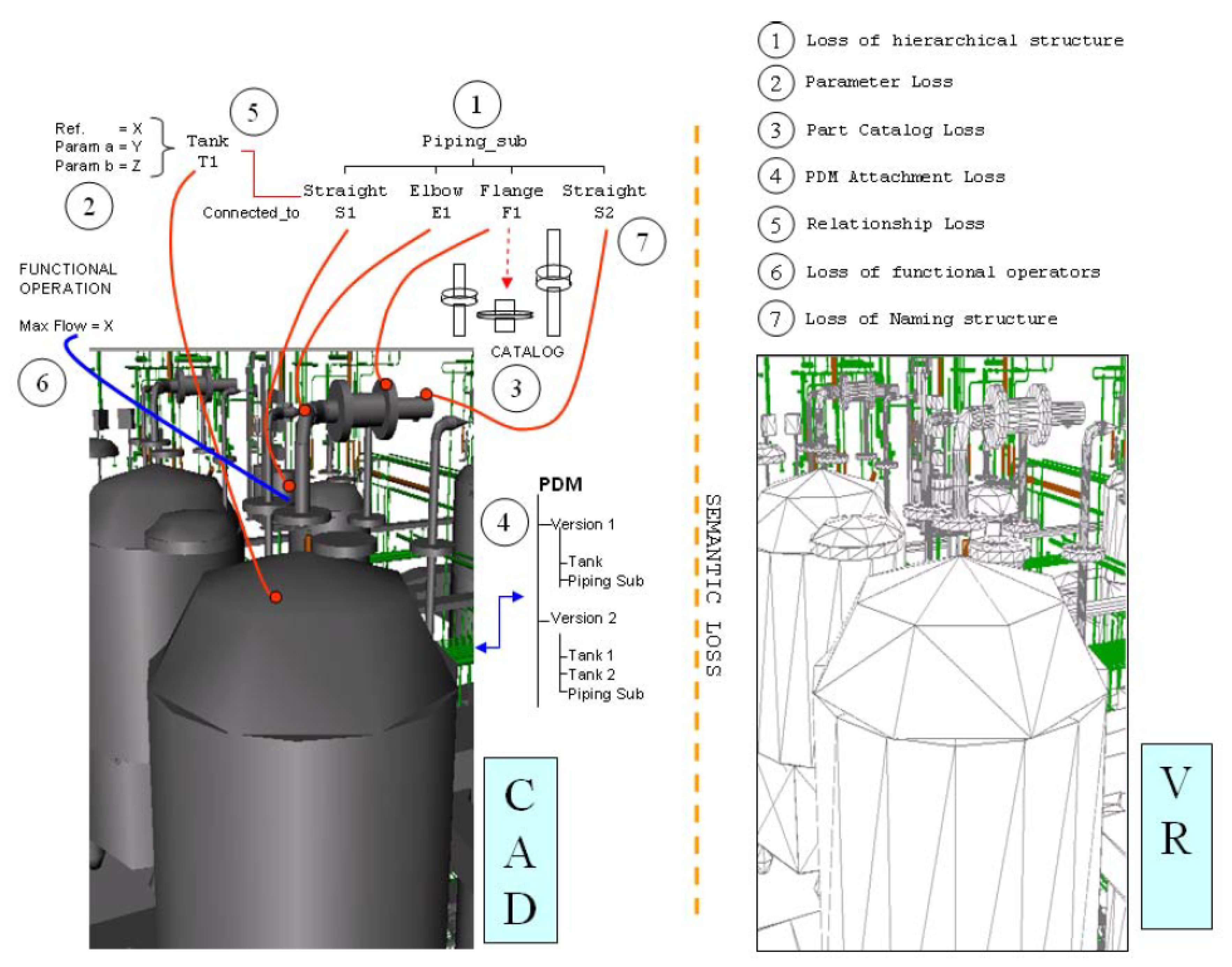
Several problems arise from the export of 3D CAD models to STEP or IGES standards. These problems are not intrinsically related with the ISO STEP [3] specification, but to the implementation of the export functionalities in the most common CAD systems. Most of them are related to the “semantic loss”, as originally formalised by Posada [6]. This includes losses of hierarchical structure, parameters, part catalogue information, PDM attachment, relationships, functional operators and naming structure, among others (Figure 1).

Other kinds of problems that 3D converted files present in STEP include wrong or inappropriate geometrical or topological descriptions. Some of the most common errors that use to appear in this category are: (i) wrong description of cylindrical or rectangular holes as solid cylinders or solid cuboids, (ii) description of simple geometric primitives in terms of more complex structures: a typical case is the conversion of Cylinders, Cones, Toroid sections, or Planar FACES to non-uniform rational basis spline curves (NURBS), adding unnecessary complexity to the converted model, and (iii) conversion of auxiliary structures used in the CAD system for internal purposes as if they were intrinsic geometric parts of the 3D model (e.g., dimension LINES, axis LINES, etc.).

There are real industrial problems that originate in these conversion processes. Our proposed methodology can help the engineer or designer to tackle many of these errors, as it provides a way to specify fast geometric and topological tests that can be interactively specified. To mention a few:

• Adaptation of 3D CAD complex models for optimal visual inspection and interaction in Virtual Reality (as explained in [7]).
• Reconstruction of semantic features of converted parts (as in [8]).
• Geometric simplification of the model.
• Automatic detection of rounder corners and chamfers.
• Automatic detection of holes. This is a very relevant and frequent case, used to prepare industrial procedures, such as workpiece painting, part drilling, robotic manipulation, structural optimization, etc.

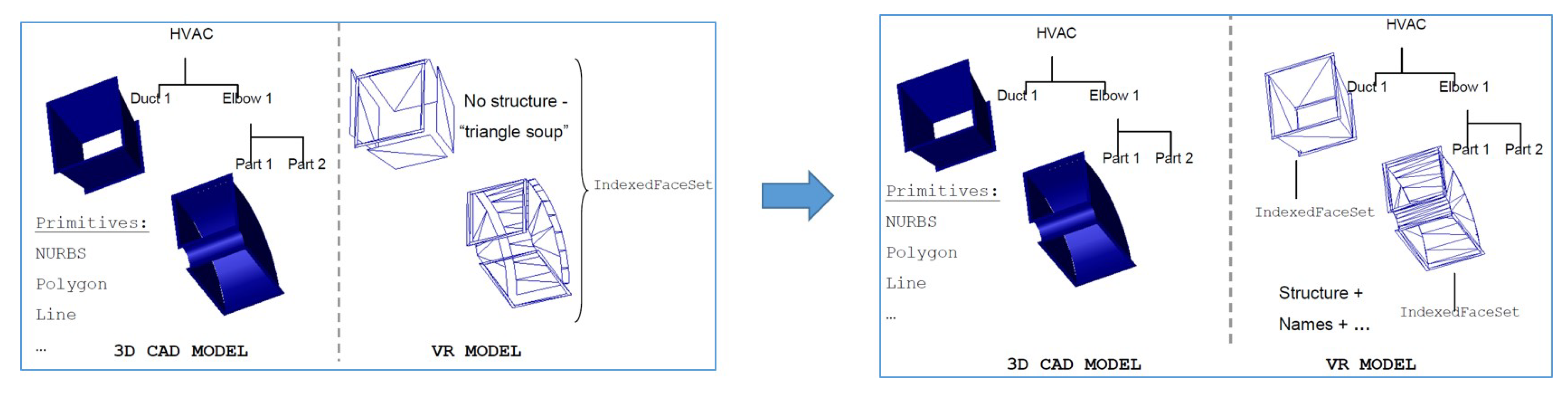
Following an early approach similar to our method, Posada et al. [5,6] showed how the problems (i), (ii), and (iii) could be solved in the context of the problems (1), (2) and (3) above, specifically in the case of large 3D CAD models of chemical plants and automotive factories (example in Figure 2), using the STEP ISO 10303-21 standard to recover structure and meaning of the models.

Our approach is more systematic in the interactive formalisation of the graph structure for the geometric pruning and it is more comprehensive in terms of the geometric filter algorithms and the support of topologic primitives.

Industrial Case

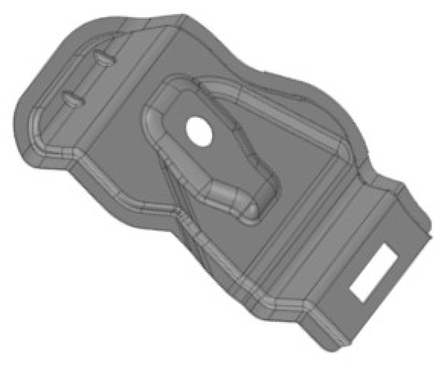
In the industrial case presented in this article, we show in detail how the problem of automatic detection of holes can be tackled with our new approach (problem 5. above). The industrial problem described is the following: a specialized engineering company handles thousands of 3D CAD models of sheet metal parts (Figure 3) for automotive and aeronautic industries. One important operation that they perform on the models is the painting planning strategy for each part, and this requires the automatic location of holes in the CAD model as a critical step. They have many providers that use different CAD systems, and they work on the common basis of the 3D CAD models exported as STEP models.

However, the reality is that many of those exported models have insufficient specification of the holes (as explained above), so the STEP model inspection has to perform a combined geometry and topology test to correctly identify the holes. For instance, a common semantic loss that appears in these models is that hole geometries and topologies are incorrectly described in the STEP file. The use of our interactive method allows for a straightforward solution the problem, since our feature recognition system was well suited for this task. It allows to perform the required test as a feature recognition task that not only identify correctly holes in well-exported models, but also overcomes potential problems in the description of some exported models. A software system implementing the presented methodology was successfully deployed at the company engineering department. We will now present our method, and show its implementation and validation results.

1.2. Literature Review

Syntactic Pattern approaches for Feature Recognition (FR) [9,10,11] use a description language based on semantic (manufacturing) primitives to express the workpiece and then compare the syntax of the primitive expression against a grammar that defines a particular feature. These approaches cover a small domain of features (2D prismatic, rotational, turning, and revolution).

Logic Rule FR [12,13,14] use a rule set that defines a particular feature, using a FACE as seed. The rules specify the number and type of bounding FACEs. These methods are more robust than Syntactic Pattern FR. However, they (a) present ambiguities in the feature definition, and (b) have a reduced domain (only prismatic solids).

Graph-based FR [15,16,17,18] creates an Attribute Adjacency Graph (AAG) which contains the topology connectivity of FACEs in a given Solid Boundary Representation (B-Rep) and matches subgraphs of the AAG to a database of diverse (feature) patterns. The shortcomings of graph-based FR are: (a) the extensive pre-processing to build the graphs representation of the workpiece and of each feature primitive, and (b) missing parts in the graph to be matched, caused by nested or inter-acting features. Positive outlooks for these methods are the new graph algorithms that apply AI (such as Hybrid Graph-Rule FR), which address interacting or nested features.

Feature Vector FR [19] extends the simple graph-based approach by applying a new EDGE classification scheme, allowing for the treatment of curved FACEs. The approach is based on a unique method to represent any given feature, called feature vector, which can be generated directly from the B-Rep modeller. The use of feature vectors in the recognition process allows for polynomial time performance for any Attribute Adjacency Graph (AAG).

Volume Decomposition FR [20,21] determines a polyhedral convex hull circumscribed around the workpiece and define the boolean differences between the convex hull and the workpiece as an alternant union or subtraction of volumes. Volume Decomposition FR is a heuristic method. Thus, there is no guarantee of the feature being correctly expressed by the volume decomposition. It is (as all FR algorithms) computationally expensive.

An Access Direction FR [22] is based on the directions from which access to the feature is possible. This particular work is implemented on STEP-based platform, thus rendering independence from proprietary formats. This approach is limited to features machinable in 3-axis centres.

Declarative Feature Language FR [1,23] defines the CAD features using a declarative language based on base entities (FACEs, EDGEs, etc...) and relations among them. Afterwards, the feature definition is translated into a database query for the CAD modeler database. A naive translation from the declarative language to the database query results in an unfeasible time complexity for any realistic number of entities, therefore, database optimization techniques are applied to reduce the time complexity of the method [1]. The main advantage of this approach lies in the superior performance with respect to other approaches when treating complex geometries and large data sets. The main disadvantage is that it relies heavily on the correctness of the CAD modeler database; therefore, incapable to treat semantic loss problems.

Another STEP-based approach is presented in [24], which describes FR with non planar surfaces (cylinder, cone, sphere, torus, B-spline, swepts). This approach is similar to Volume Decomposition in that it identifies volumes to be removed in order to manufacture the feature. The FACE and EDGE-based topological and geometrical information is collected in a first pass. In the second pass, the non-planar FACE- based featured are extracted. A drawback of this approach is that it relies on a EDGE-based search, expensive with complex curved surfaces.

Reconfigurable FR [25] obeys to the fact that a feature is an inherently subjective denomination, which may correspond to different topological/geometrical B-Rep neighborhoods, according to the field and application of the workpiece. This work presents a feature declaration language and underlying geometric reasoning server, which allow a more efficient FR, at the price of each user re-configuring his/her FR declaration and underlying filters.

1.3. Conclusions of Literature Review

Generally, previous approaches to the Feature Recognition problem present three major shortcomings: (i) a reduced domain of application, mostly restricted to boolean combinations of prismatic shapes or turning parts; (ii) reliance on FACE or EDGE search and classification, therefore excluding other useful geometric information; and, (iii) inability to treat the semantic loss problem in STEP-based methods. The interested reader may refer to the survey in Ref. [26], to complement our review.

In response to some of the existing shortcomings in FR, here we present the design and implementation of an interactive re-configurable graph search method for FR. Our approach prunes the B-Rep search space with user-prescribed geometric tests. An early reduced version of this work is presented in the short paper [2]. Therefore this manuscript is an extension of [2] with considerable additional contributions. The present manuscript contains the following elements, absent in [2]: (i) analysis of the industrial relevance of the approach, (ii) complexity analysis of the algorithm, (iii) details about the implementation and the Graphic User Interface for interactive Feature Recognition, (iv) search graph construction strategies, (v) additional curvature-based geometric filters, and (vi) industrial instancing with more examples. In the current manuscript, we fully discuss the construction methodology for the search graph structure and introduce the curvature-oriented geometric filters that allow for curved-geometry identification. In [2], we discussed the method’s performance with respect to the number of nodes in the search graph. In the current manuscript, we extend such discussion to include a complexity analysis of our method. Our approach admits topologies of the types 0 (VERTEX), 1 (EDGE or LOOP), and 2 (FACE or SHELL). It is implemented on STEP [3] B-Rep standard, which facilitates its migration to other modelers.

2. Materials and Methods

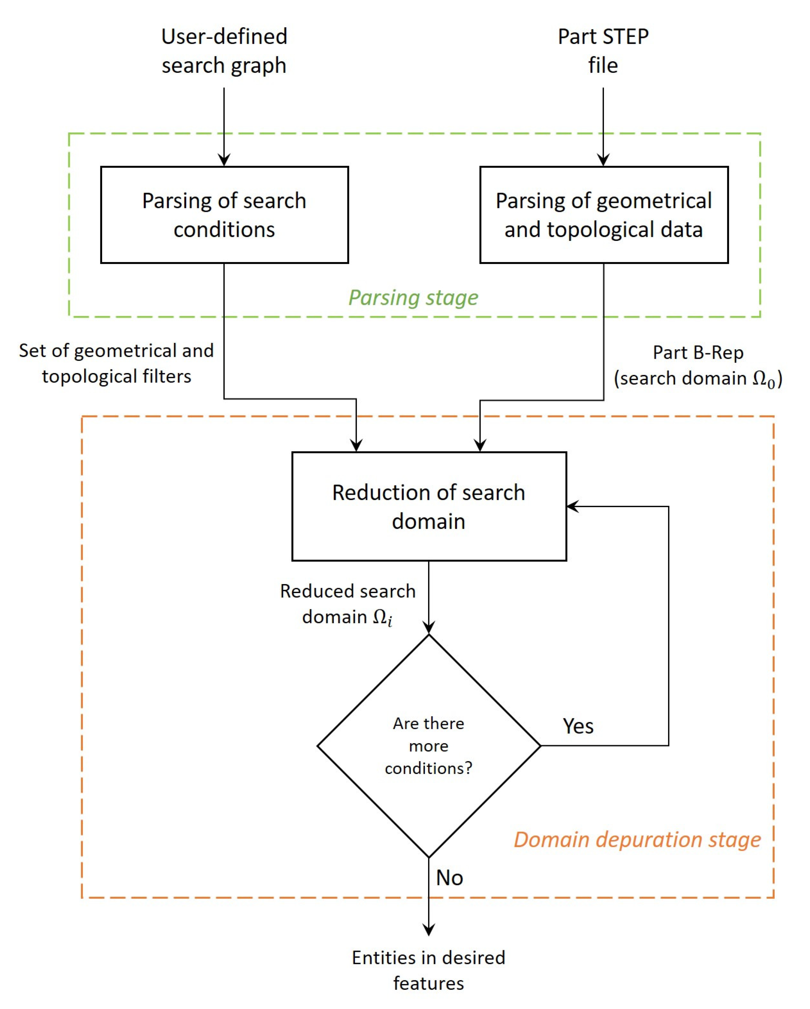
Our implementation includes a Parsing stage and a Domain Depuration stage, as follows (Figure 4).

Parsing stage. This stage parses two inputs: (a) an user-defined unstructured search graph, and (b) part STEP file containing geometry and topology information of the workpiece. Process (a) is written in C++ and translates into a graph structure of geometrical tests which includes the target topologies. The test enforcement order is implicit in the pruning graph structure. In the parsing stage, each pruning node is equipped with geometry or topology boolean test functions. At the domain depuration stage, the relevant test is triggered and a boolean FALSE would result in the elimination of the tested topologies from the search space. In this manner, the FR parsing stage produces the pruning test graph, with its nodes loaded with the geometry test functions and pruning actions, Process (b) part STEP file parsing is achieved by using Open Cascade [RC12] platform. The Open Cascade Processor populates a Boundary Representation (B-Rep) database by parsing the workpiece STEP file, thus producing the initial search domain ${\Omega }_0$.

Domain Depuration stage. This stage executes upon the B-Rep ${\Omega }_0$ domain the boolean tests implicit in the pruning graph, progressively reducing the domain. Following the graph structure of the pruning process, the output of a pruning node is the input of the following one. The geometrical/topological condition of the current iteration is applied to all target topologies of the current search domain and those topologies who fail the test are purged from the search domain, hence reducing its size in after enforcing each node conditions. Once all conditions in the sequence are enforced, the resulting search domain corresponds to the topologies that constitute the desired features.

2.1. Search Graphs

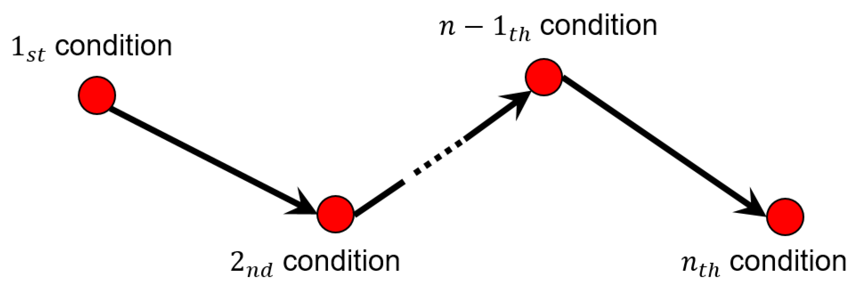
A domain pruning graph is a directed acyclic graph (DAG). Although in many cases this pruning graph is a simple sequence (i.e., a chain), it must be realized that more involved domain reductions require general DAGs. Each node in such graphs contains the specification of the topologies to be tested and the nature of the test. The DAG for search domain pruning is general enough to allow diverse boolean test sequences. However, as said before, in the majority of cases the manufacturing engineer or technician specifies a chain sequence (e.g., Figure 5).

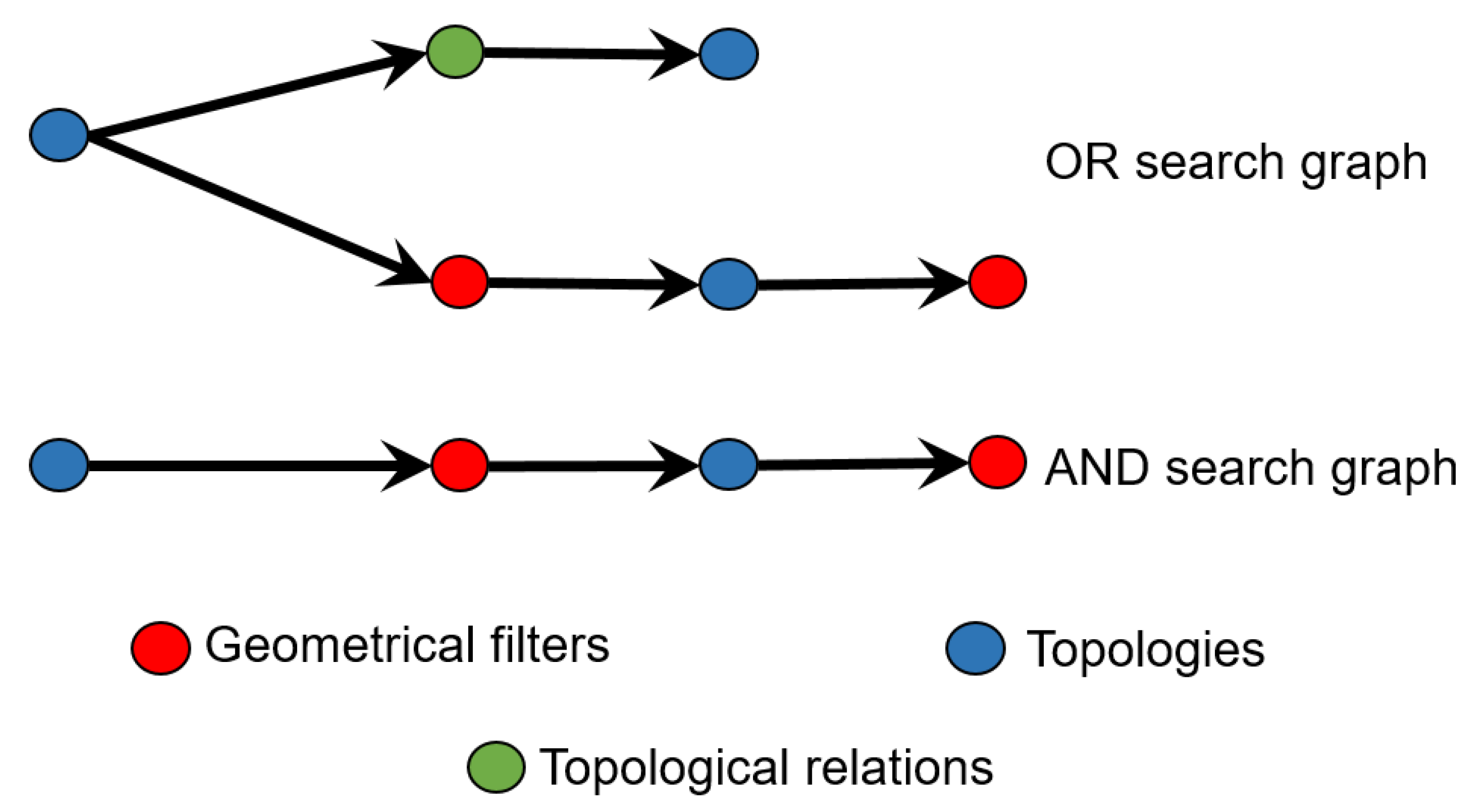
In a Domain Pruning Graph, nodes can be classified into three types: (1) Topologies, (2) Geometry Tests, and (3) Topology Tests. (1) Topologies are the 0-, 1-, and 2-manifold sets SHELL, FACE, LOOPE, EDGE, VERTEX, represented by Programming Objects or classes. (2) Geometry Tests are the boolean queries responded by querying the underlying Geometries of the Topologies (Parametric Surfaces and Curves, and Points). (3) Topology Tests are also boolean queries, stated on one or more Topologies, which are not solved by geometric arguments. An approximate grammar for a Pruning Graph is:

$$\begin{array}{cc}\hfill & <pruning\_graph>⟶<serial\_test>AND<pruning\_graph>\hfill \\ \hfill & <pruning\_graph>⟶<serial\_test>\hfill \\ \hfill & <serial\_test>⟶<atomic\_test>OR<serial\_test>\hfill \\ \hfill & <serial\_test>⟶<atomic\_test>\hfill \\ \hfill & <atomic\_test>⟶<topology\_test>|<geometry\_test>\hfill \\ \hfill & <topology\_test>⟶<topology><topo\_relation><topology>\hfill \\ \hfill & <topology>⟶SHELL\left|FACE\right|LOOP\left|EDGE\right|VERTEX\hfill \\ \hfill & <topo\_relation>⟶CONTAINED\left|CONTAINS\right|IS\_ADJACENT\hfill \\ \hfill & <geometry\_test>⟶<topology><geometry\_property>\hfill \\ \hfill & <geometry\_test>⟶<topology><geometry\_property><topology>\hfill \\ \hfill & <geometry\_test>⟶<topology><geometry\_property><value>\hfill \\ \hfill & <geometry\_property>⟶CYLINDRICAL\left|CIRCULAR\right|PARALLEL\hfill \\ \hfill & PLANAR|DEAD\_END\hfill \\ \hfill & <value>⟶<real\_number>\hfill \end{array}$$

It must be stated that, in our implementation, this grammar is implemented by driving the user actions through the Graphic User interface and not by parsing a description file (although it would be also possible).

Figure 6 presents examples of pruning graphs built while using the grammar mentioned above. Notice that the effectiveness in reducing the search space directly depends on the precision and consistency of the pruning graph. An inconsistent graph would end in a null solution space, independent from what ${\Omega }_0$ is. A too lax pruning graph would allow for a large search space, thus failing to execute FR.

2.2. Topology-Geometry Data Structure

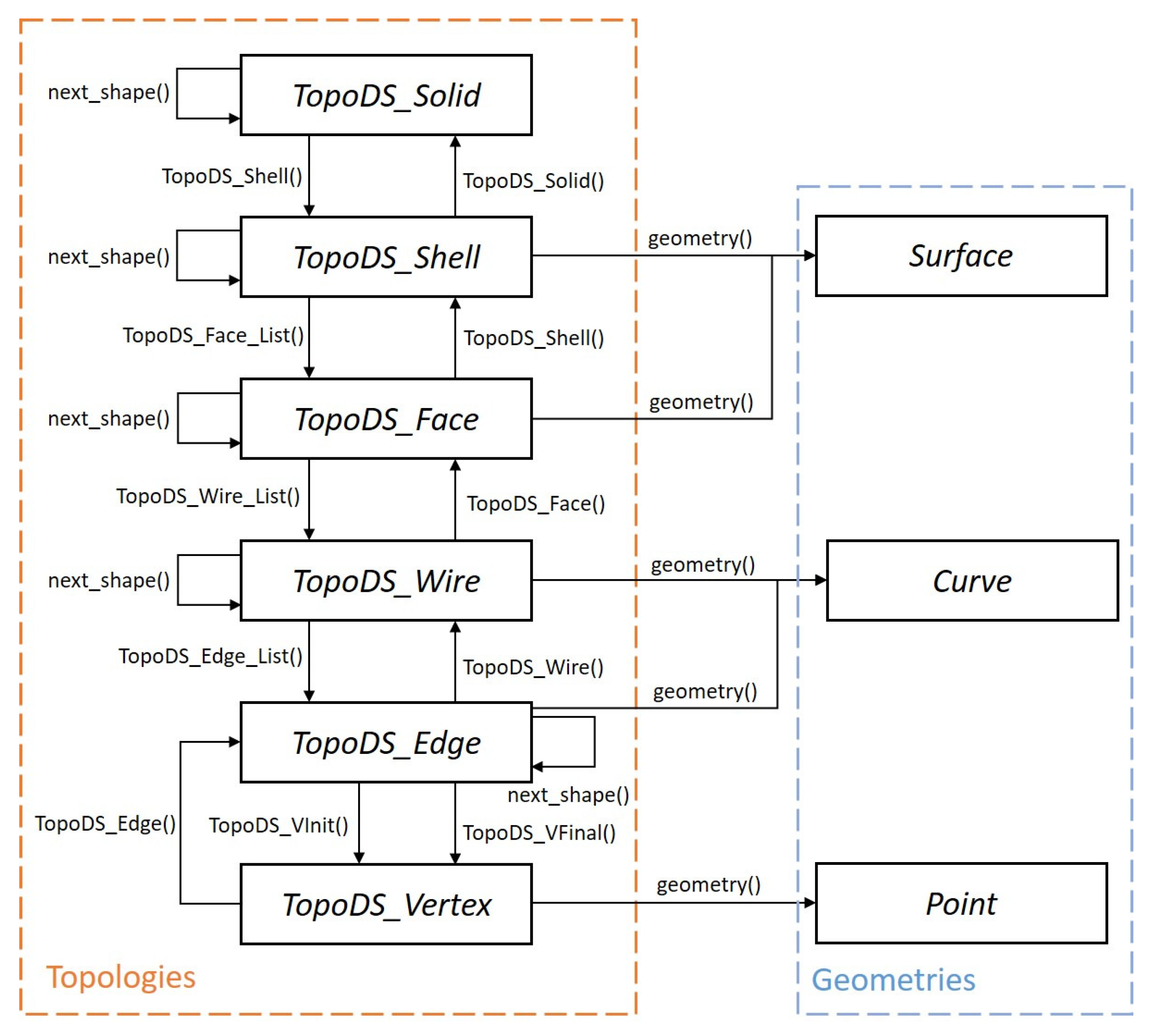
A geometry-topology data structure is needed to efficiently store and manage all geometric and topological information of the solid workpiece in order to explore and reduce the search domain. The data structure implemented is based on the OpenCascade [27,28] platform and it resembles a B-Rep data structure. Figure 7 shows the implemented data structure.

The hierarchical organization of the data structure allows for exploration of the topology-space of the workpiece and access to the geometrical properties of any topology. As usual, Topology connectivity relations among entities, while Geometry refers to positions, sizes, and underlying shapes. Geometric filters are applied on geometrical entities, not directly on topologies. Therefore, access to the geometric entities underlying the topologies is required to apply the geometric filters. All geometry and topology classes are derived from the base TopoDS class in the OpenCascade^TM library.

2.3. Topological Relations

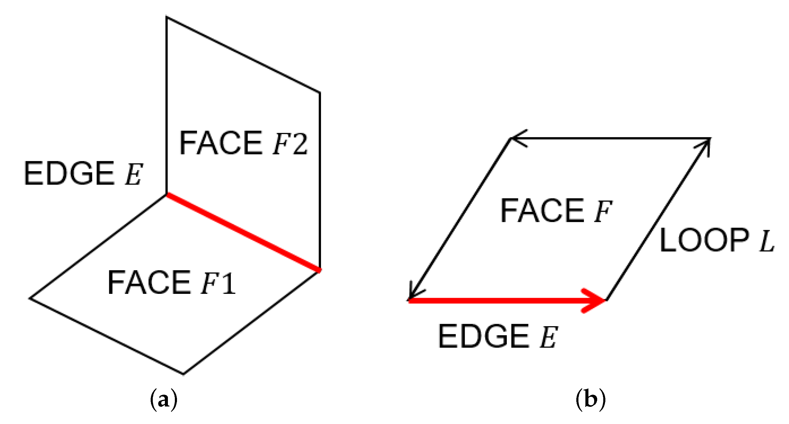
Topological Tests assess whether the given topologies comply with the inquired role (CONTAINED, CONTAINS, IS_ADJACENT). These interrogations are answered using the structure implicit in the B-Rep data structure (Figure 7), instanced in the particular workpiece at hand. Figure 8 shows examples of the implemented topological tests.

Figure 8a shows the adjacency relation, which determines whether two FACEs are adjacent to each other (i.e., their border LOOPs share an EDGE). Figure 8b shows the containment relation, which determines whether an EDGE is contained in any of the border LOOPs of the given FACE. This test is also applied to LOOPs containing an EDGE. The use of topological relations in the search graph allow for greater flexibility in the FR process taking advantage of the hierarchical organization of topologies and their relations to one another.

2.4. Geometrical Filters

Geometrical Filters assess whether or not a subset of the B-Rep satisfies a given geometric condition. Failure to pass the filter eliminates such a B-Rep subset from the search space, therefore, reducing the search space for the next filters. New geometrical tests specially suited to treat curved geometries underlying 2- and 1-topologies are required to identify features containing curved geometries. Examples follow.

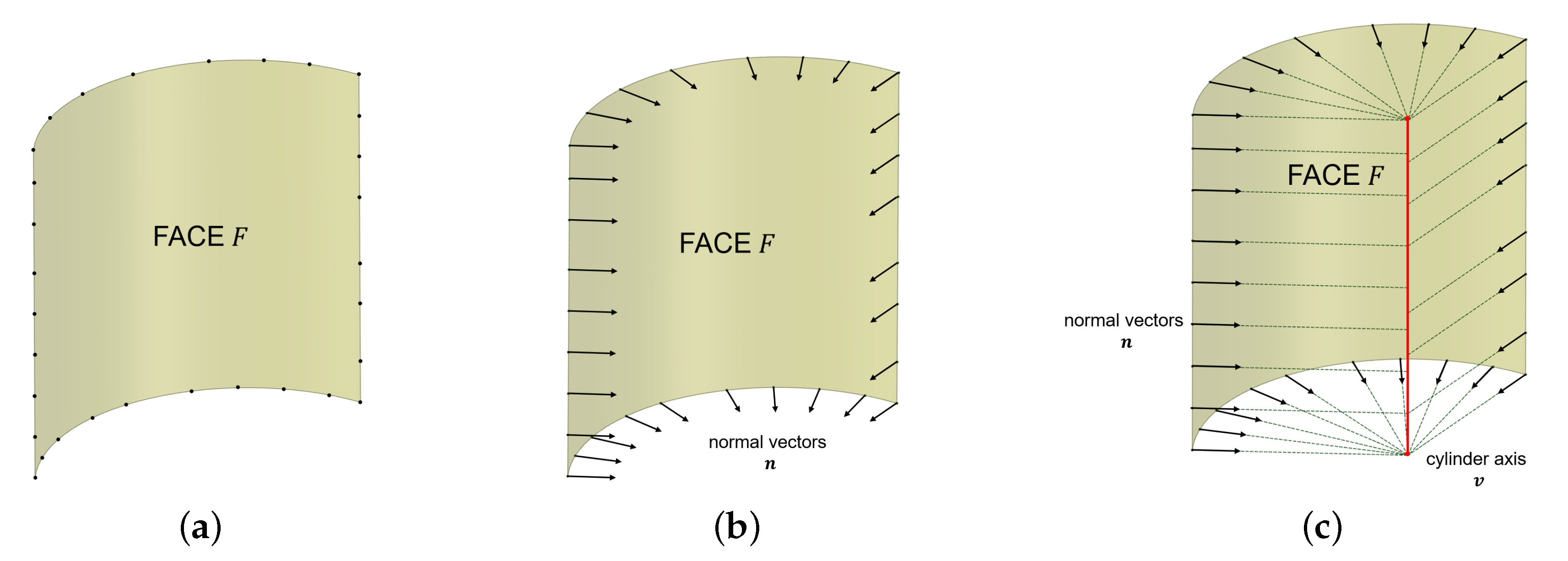
2.4.1. Cylindrical FACE Test

The goal of this test is to determine whether a FACE topology is carried by a cylinder geometry (within user-specified error margins). Ruiz et al. proposed the method in use [29], and it goes as follows (Figure 9):

Denote $\overrightarrow{P}$ as the set of Points in the underlying surface of a FACE topology:

• For each point $p\in \overrightarrow{P}$, calculate the normal vector $\overrightarrow{n_p}$ of a plane tangent to the surface in p.
• By crossing each other two line segments defined by a point and its associated normal vector, a set of points $\overrightarrow{C_p}=\left\{q_1,q_2,q_3,\dots \right\}$ near the cylinder’s axis $\overrightarrow{v}$ is obtained. Notice that, even when two line segments do not intersect, a crossing point can still be obtained as the midpoint of the line segment corresponding to the shortest distance between the two initial line segments.
• The technique of Principal Component Analysis (PCA) is used to obtain an approximation of the cylinder’s axis $\overrightarrow{v}$ and its pivot point $v_p$ from set $\overrightarrow{C_p}$.
• For each point $p\in \overrightarrow{P}$, the distance to the cylinder’s axis $\overrightarrow{v}$ is calculated. The surface resembles a cylinder if all calculated distances are similar within a specified tolerance range.

2.4.2. Circular EDGE Test

Using a similar strategy, the goal of this test is to determine whether an EDGE topology is carried by a circle geometry (within user-specified error margins). The method in use is a modification of the method that was proposed by Ruiz et al. [29]:

Denote $\overrightarrow{P}$ as the set of Points in the underlying curve of an EDGE topology:

• For each point $p\in \overrightarrow{P}$ calculate the normal vector $\overrightarrow{n_p}$ of a plane tangent to the curve in p.
• By crossing each other two line segments defined by a point and its associated normal vector, a set of points $\overrightarrow{C_p}=\left\{q_1,q_2,q_3,\dots \right\}$ near the circle’s origin O is obtained. In this case, any two line segments will always intersect, since they are coplanar.
• The circle’s origin O is defined as the point which coordinate values are the average values of the coordinates of points in set $\overrightarrow{C_p}$.
• For each point $p\in \overrightarrow{P}$, the distance to the circle’s origin O is calculated. The curve resembles a circle if all the calculated distances are similar within a specified tolerance range.

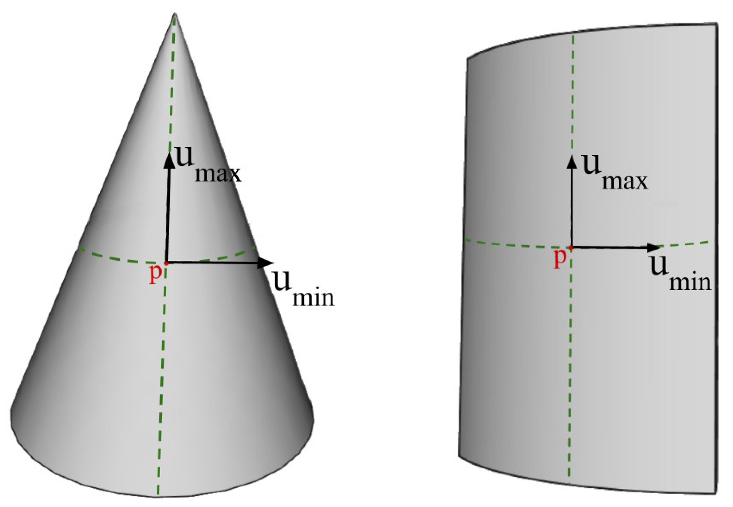
Another set of implemented geometrical filters is based on the surface curvature supporting the FACE topology (Figure 10). For every point of the surface is possible to compute the principal curvatures values ${\kappa }_{max}$, ${\kappa }_{min}$ and directions $\overrightarrow{u_{max}}$, $\overrightarrow{u_{min}}$, which are descriptors of how much and in which directions the surface bends in a specific location [30]. Different conditions on those geometric entities can be tested to identify the underlying nature of the surface [31]. Additionally, in the spherical and cylindrical surface tests, it is possible to define an optional constraint on the value of the curvature radius. All of the following tests are implemented in the Geomlib SDK [32] and they are based on the OpenCascade library.

2.4.3. Planar FACE Curvature Test

The goal of this test is to determine whether the FACE topology is carried by a planar geometry. For every point of a plane, the two principal curvature values are equal to zero and the normal vector is constant in direction and orientation. Denote $\overrightarrow{P}$ as the set of points obtained by sampling the surface continuous parametric $uv$ space with $u_{samples}$ and $v_{samples}$ number of samples in the two dimensions.

• For each point $p\in \overrightarrow{P}$, calculate the normal vector $\overrightarrow{n_p}$ of a plane tangent to the curve in p.
• For each point $p\in \overrightarrow{P}$ calculate the principal curvature values ${\kappa }_{p\_min}$ and ${\kappa }_{p\_max}$.
• The underlying geometry is planar if $\overrightarrow{n_p}=const$, ${\kappa }_{p\_min}=0$ and ${\kappa }_{p\_max}=0$ for every $p\in \overrightarrow{P}$ within a specified tolerance range.

2.4.4. Spherical FACE Curvature Test

The goal of this test is to determine whether the FACE topology is carried by a spherical geometry. For a sphere the two principal curvature values are equal and constant and not zero throughout all the surface. Denote $\overrightarrow{P}$ as the set of points obtained by sampling the surface continuous parametric $uv$ space with $u_{samples}$ and $v_{samples}$ number of samples in the two dimensions.

• For each point $p\in \overrightarrow{P}$, calculate the principal curvature values ${\kappa }_{p\_min}$ and ${\kappa }_{p\_max}$.
• The underlying geometry is spherical if ${\kappa }_{p\_max}={\kappa }_{p\_min}=const$, ${\kappa }_{p\_min}\ne 0$ and ${\kappa }_{p\_max}\ne 0$ for every $p\in \overrightarrow{P}$ within a specified tolerance range.
• Optionally compute the radius of curvature $R_p=\frac{1}{{\kappa }_{p\_max}}$ and control that is equal to a specified value within a tolerance range

2.4.5. Cylindrical FACE Curvature Test

The goal of this test is to determine if the FACE topology is carried by a cylindrical geometry. Differently from the previous tests, in this one, we also take into consideration the direction of the principal curvatures. As a matter of fact, for every point of a cylinder, the minimum curvature direction is constant and its corresponding value is zero, while the maximum curvature is constant and different from zero. An additional condition on the curvature radius is imposed to distinguish the geometry from a cone or a free-form surface. Denote $\overrightarrow{P}$ as the set of points obtained by sampling the surface continuous parametric $uv$ space with $u_{samples}$ and $v_{samples}$ number of samples in the two dimensions.

• For each point $p\in \overrightarrow{P}$ calculate the principal curvature values ${\kappa }_{p\_min}$, ${\kappa }_{p\_max}$ and directions $\overrightarrow{u_{p\_min}}$, $\overrightarrow{u_{p\_max}}$.
• Test for all of the points that the minimal curvature direction $\overrightarrow{u_{p\_min}}$ is constant, its corresponding value ${\kappa }_{p\_min}$ is zero and the maximum curvature value ${\kappa }_{p\_max}$ is constant and different that zero within a specified tolerance range.
• For each point $p\in \overrightarrow{P}$, compute the radius of curvature $R_p=\frac{1}{{\kappa }_{p\_max}}$.
• Test that the radius is constant throughout all the surface $R_p=const$ within a specified tolerance range.
• Optionally control that the radius of curvature $R_p$ is equal to a specified value within a tolerance range.

2.4.6. Conical FACE Curvature Test

The goal of this test is to determine whether the FACE topology is carried by a conical geometry. The procedure is similar to the previous one but with no curvature radius test and an additional fitting stage. Denote $\overrightarrow{P}$ as the set of points obtained by sampling the surface continuous parametric $uv$ space with $u_{samples}$ and $v_{samples}$ number of samples in the two dimensions. Additionally, define a smaller set of points $\overrightarrow{P_{sub}}\in \overrightarrow{P}$ obtained with an evenly spaced sub-sampling of $\overrightarrow{P}$. It is important that this set is small in order to ensure that the execution time remains small.

• For each point $p\in \overrightarrow{P}$ calculate the principal curvature values ${\kappa }_{p\_min}$, ${\kappa }_{p\_max}$ and directions $\overrightarrow{u_{p\_min}}$, $\overrightarrow{u_{p\_max}}$.
• Test for all the points that the minimal curvature direction $\overrightarrow{u_{p\_min}}$ is constant, its corresponding value ${\kappa }_{p\_min}$ is zero and the maximum curvature value ${\kappa }_{p\_max}$ is constant and different that zero within a specified tolerance range.
• For each point $p\in \overrightarrow{P}$ compute the radius of curvature $R_p=\frac{1}{{\kappa }_{p\_max}}$ and test that its value is not constant within a specified tolerance range.
• Use the RANSAC algorithm [33] to fit a cone to $\overrightarrow{P_{sub}}$. If the algorithm succeeds the FACE supports a conical geometry.

2.5. Complexity and Performance

The overall performance of the presented methodology is mainly influenced by two aspects: (i) the number of entities in the model and (ii) the number of nodes in the search graph and the performance of the filter itself. Regarding the number of entities, a larger model will negatively impact the performance of the algorithm, since the initial search domain is larger and requires more evaluations of the geometric filter in each step of the search process. One must understand the trade-off that takes place to assess the performance consequences of introducing new nodes to the search graph: a new filter adds new operations to the execution sequence and at the same time reduces the search domain for the next filter. Thus, if a new filter is inserted in the search graph, in general the subsequent filters will experience a reduction of the number of operations to perform, since the search domain is reduced by the insertion of the new filter. Therefore, adding a new filter might actually improve performance if the number of saved operations is larger than the number of operations added by the insertion of the new filter. The type of filter is also important to assess performance, since not all filters reduce the search domain by the same amount and this depends on the characteristic of initial data and desired feature. Therefore, adding a filter with high reduction somewhere in the search graph will have positive effects on the performance of the algorithm.

The currently accepted theoretical algorithm for the graph isomorphism problem (which is the underlying problem in most of the methods found in literature) has a time complexity of $2^{O\left(\sqrt{nlogn}\right)}$ [34]. More recently, a quasipolynomial time algorithm [35] was announced with a time complexity of $2^{O\left({\left(logn\right)}^c\right)}$ for some fixed $c>0$.

In order to calculate the time complexity of our algorithm, we assume a survival rate $\alpha$, which is, after each iteration $\alpha$ percent of entities survive the filter. We denote n as the length of the initial geometry-topology data and M the number of filters in the search graph. We assume the filters to be a constant-time operation, since it is applied to an individual topology and does not depend on the length of the initial data set. Time complexity T of the algorithm is then estimated as:

$$T\left(n,M\right)={\alpha }^{0}n+{\alpha }^{1}n+{\alpha }^{2}n+{\alpha }^{3}n+\dots +{\alpha }^{M}n$$

(1)

Subsequently, we can express the time complexity of the algorithm as:

$$T\left(n,M\right)=O\left(Mnlogn\right)$$

(2)

In order to compare the computational resources savings of our method with respect to other approaches found in literature,

Table 1. Time complexity comparison between Feature Recognition (FR) approaches for a model with n entities.

Method	Claimed Complexity	References	Comments
Graph Matching	$O\left(n^k\right)$	[1,36]	k: number of nodes in feature graph
Feature Vector	$O\left(n^3\right)$	[19]	Requires additional geometric processes that may affect performance
Volume Decomposition	$O\left(n^k\right)$	[36]	k: number of cells generated for each feature
Naive Language	$O\left(n^k\right)$	[37]	k: number of entities in the feature
Optimized Language	$O\left(n\right)$	[1,23]	Linear Complexity is achieved only for simple features
Our method	$O\left(Mnlogn\right)$	Current Manuscript	M: number of filters in the search graph.

summarizes the time complexity of different methodologies. Notice that complexities are expressed for a model of n entities, but the basic operation used to measure complexity in each method may be different; or the method could require additional processes not taken into account in the complexity measurement.

2.6. Graphic User Interface

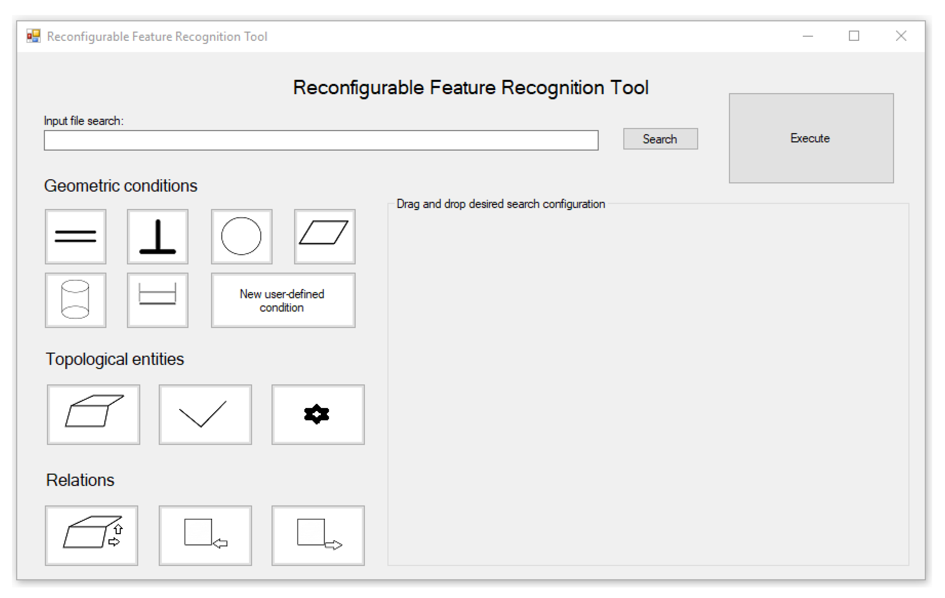
The proposed method has been implemented in an industrial environment while using a Graphic User Interface (GUI) based on icon graphs for the search graph construction with default pre-programmed geometrical filters. The GUI allows for further user customization by allowing the expansion of the geometrical filters library. Figure 11 shows the Graphic User Interface developed while using C++ graphic libraries.

The GUI consists of two panels: left panel contains the graphic icons for the topologies, geometric filters, and topological relations currently implemented, the right panel is an interactive environment where the user can drag and drop the desired icons to build a search graph following the previously presented rules. The Graphic User Interface (GUI) includes, as usual, the functionality to import a neutral format part file (STEP [3]). At the present time, our application does not import IGES [4] format.

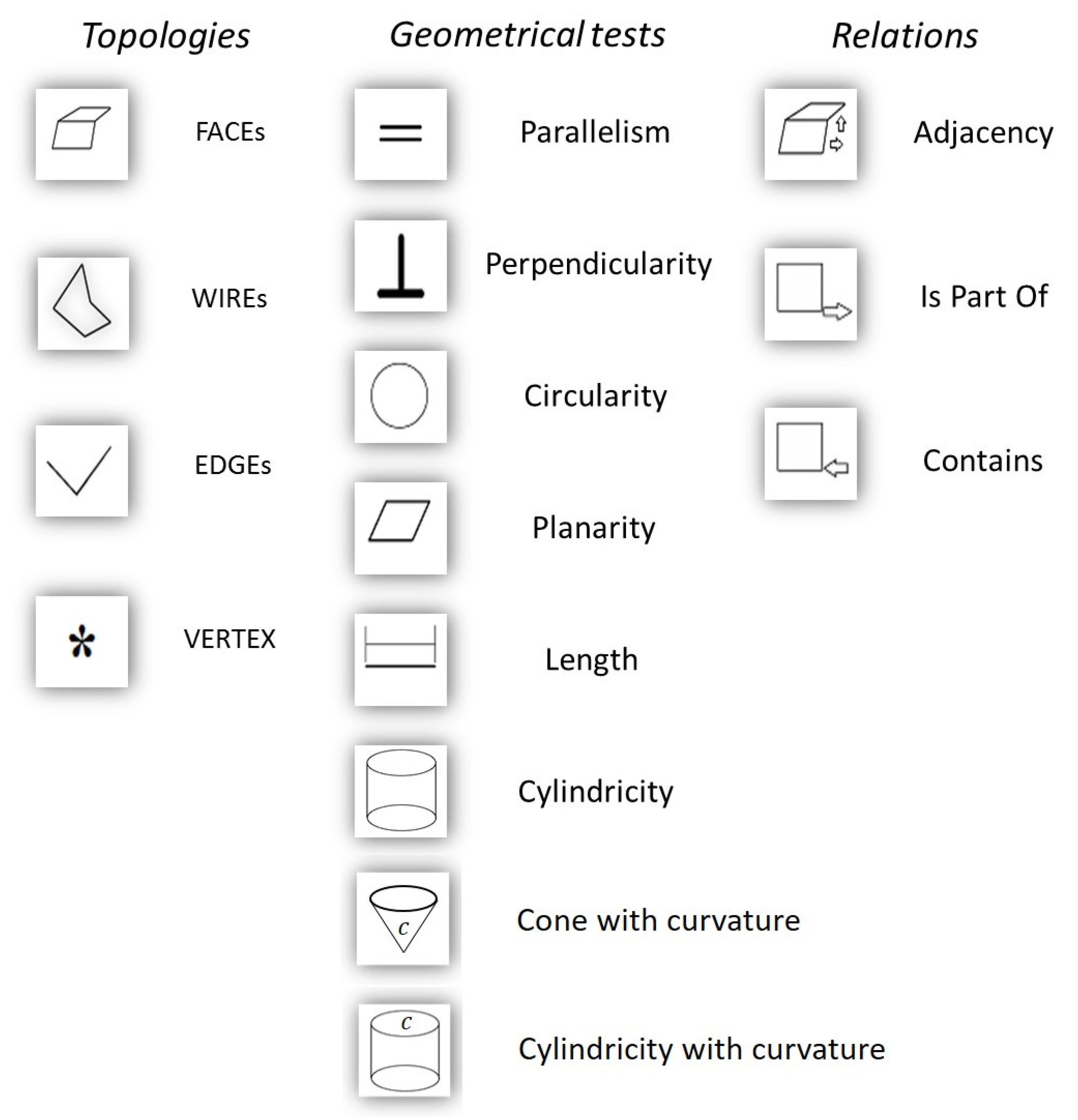
Figure 12 shows the topologies, topological relations, and geometrical tests currently implemented in the industrial instancing. This library can be further expanded by the user using DLLs to link personalized geometrical filters or topological relations.

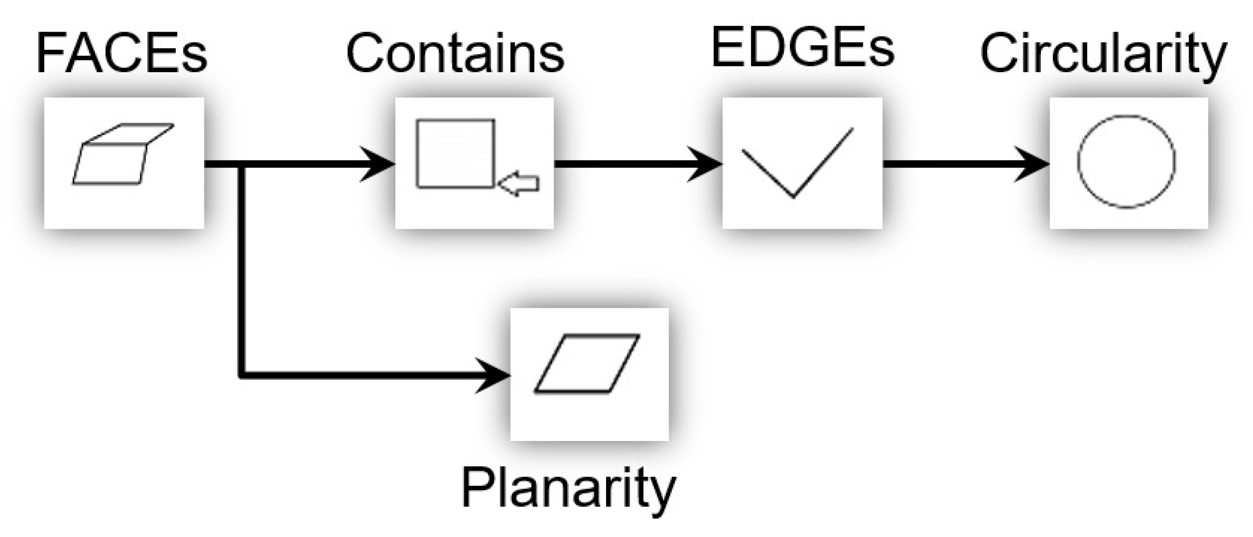
Figure 13 shows an example of a search graph built using the graphical tool. The GUI does not actively enforce the search graph construction rules, therefore, check of search graph structure validity is left to the user. Figure 14, Figure 15, Figure 16 and Figure 17 show the output of the Graphical User Interface after running the feature identification process.

3. Results

To test our interactive FR method, we present four application examples in different workpieces, as shown in Figure 14, Figure 15, Figure 16 and Figure 17. In the first two examples, the goal is to identify circular hole features on metal sheet workpieces given that the thickness of the sheet is known. In the third example, the goal is to identify square hole features on a metal sheet workpiece, also with the thickness of the sheet as known data. In the last use case the goal is to identify the chamfer surface of a car disc brake holes, i.e., the conical surface situated on top of the hole cylinders. In the presented examples, we choose a search graph strategy that includes a known dimension (thickness in this case) because it suits our available data, other search graph strategies could be used to execute the FR process for the same feature. Initial search space is denoted as ${\Omega }_0$ in all cases.

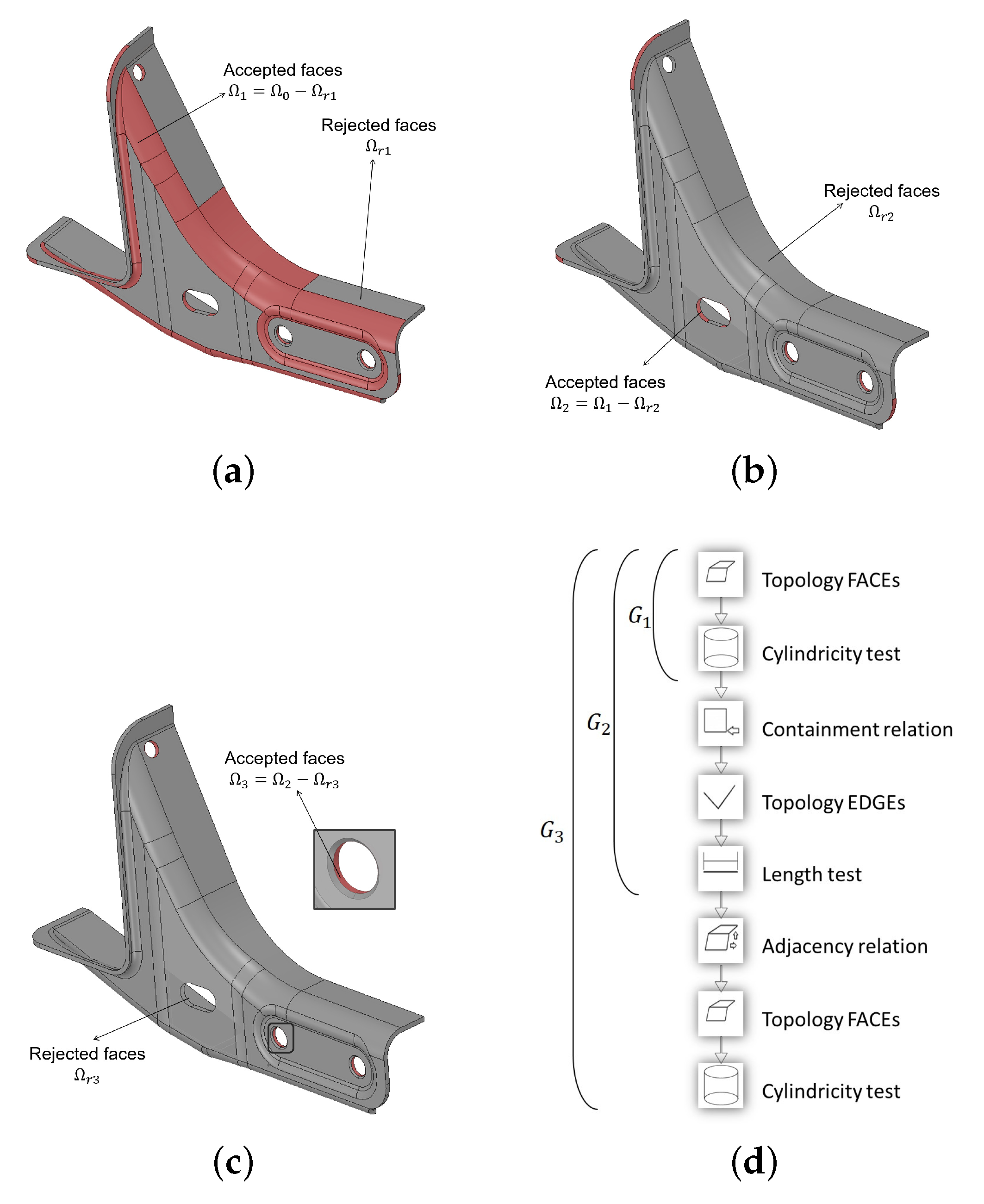
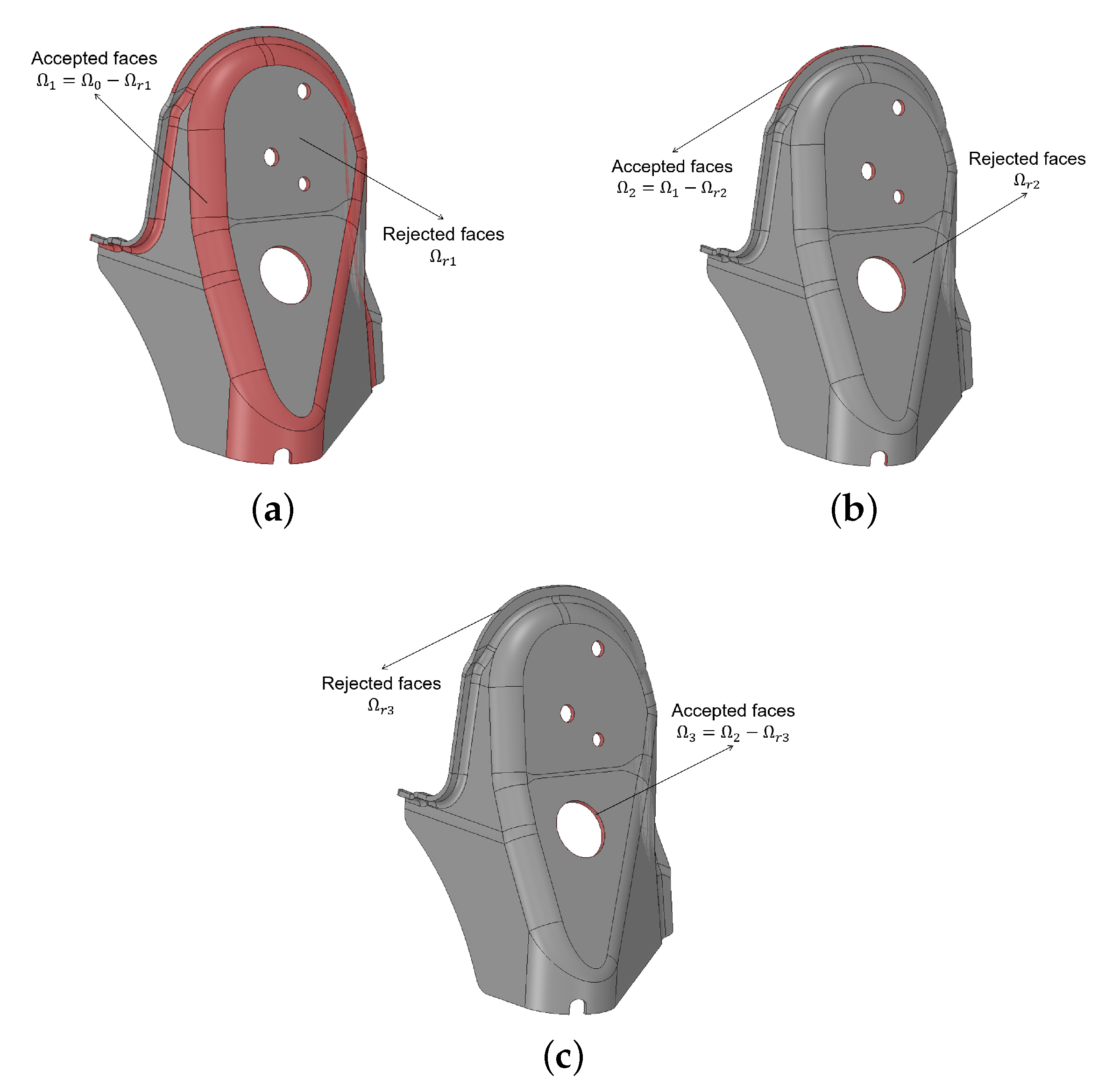
The reduced domain ${\Omega }_1$, as shown in Figure 14a and Figure 15a, is the result of pruning the correspondent initial search space ${\Omega }_0$ with the geometric filter configuration in search graph $G_1$, as shown in Figure 14d (for both data sets). The search graph $G_1$ applies the CYLINDRICITY condition to all FACEs in the domain ${\Omega }_0$. Therefore, the reduced domain ${\Omega }_1$ should only contain cylindrical FACEs, as shown in Figure 14a and Figure 15a.

The search graph $G_2$ (Figure 14d) is an extension of graph $G_1$; therefore, further pruning domain ${\Omega }_1$ by applying extra geometric filters according to the configuration of graph $G_2$. Graph $G_2$ preserves from domain ${\Omega }_1$ all FACEs that are related to an EDGE with a length value specified by the user; in this case, the specified length value is the sheet’s thickness t. Resulting reduced domain ${\Omega }_2$, only contains cylindrical FACEs related to an EDGE of length t, as shown in Figure 14b and Figure 15b.

The domain ${\Omega }_2$ contains the desired hole features and other undesired FACEs, therefore, an additional condition is necessary to prune undesired FACEs from domain ${\Omega }_2$. Search graph $G_3$ (Figure 14d) is an extension of search graph $G_2$ and further prunes domain ${\Omega }_2$ by only preserving FACEs that are adjacent (share and EDGE with) to a cylindrical FACE in ${\Omega }_1$. Hence, applying the conditions that result from graph $G_3$ to the domain ${\Omega }_2$, results in a reduced domain ${\Omega }_3$ (Figure 14c and Figure 15c) only containing FACEs of hole features, ending the process with the desired FACEs. Notice that the further pruning applied by graph $G_3$, successfully removes the undesired FACEs because of the configuration of these particular hole features. In this cases, hole features are composed of two opposed cylindrical faces (as shown in Figure 14c and Figure 15c), but is not a general rule for hole features in all cases.

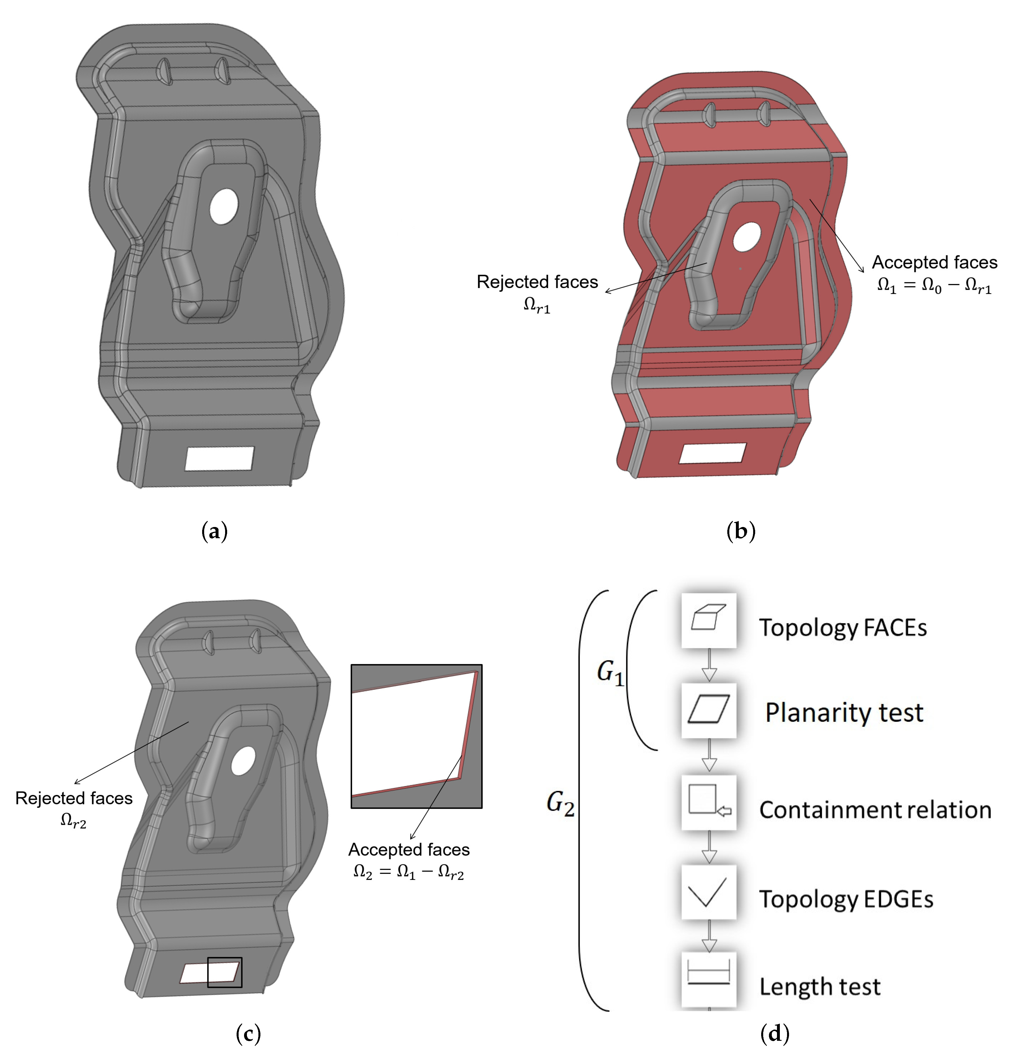
In a similar fashion, we present the result of square hole recognition in a sheet metal part in Figure 16. Figure 16a shows the initial data set ${\Omega }_0$ and we follow the same search graph strategy from FR in Examples 1 and 2, only changing the CYLINDRICAL geometric filter for the PLANAR geometric filter. Figure 16d shows the domain ${\Omega }_1\subset {\Omega }_0$ consisting of all planar FACEs present in initial domain ${\Omega }_0$ (FACE planar geometric filter). Figure 16c shows the domain ${\Omega }_2\subset {\Omega }_1$ consisting of all FACEs part of the square hole feature; domain ${\Omega }_2$ preserves from domain ${\Omega }_1$ all FACEs which are related to an EDGE with a length value specified by the user; in this case, the sheet’s thickness t. FR for square holes is successfully executed on data set 3.

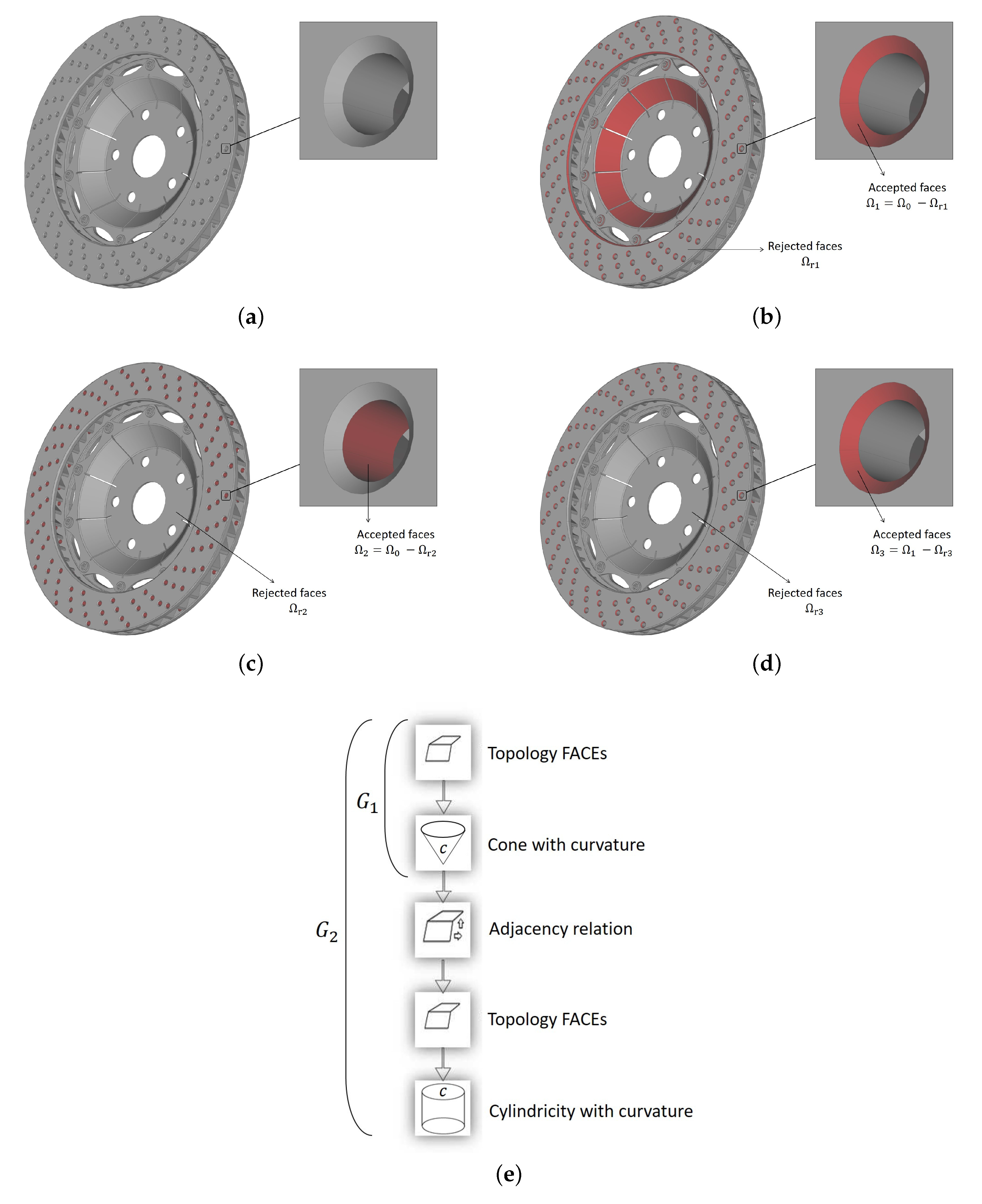
Following the same concepts of previous examples, Figure 17 shows the process to identify the chamfer surface of all countersunk holes drilled in the object. The model was taken from dataset [38], and is a disc brake of a car. In this case, the search graph is composed of a cone surface test by curvature to isolate all conical FACEs, followed by an adjacency test to all cylindrical FACEs with a known radius, also done with curvature analysis. This reflects the fact that the target surfaces are always situated on top of the hole cylinders. Figure 17a represents the initial data set ${\Omega }_0$, while, in Figure 17b, we have the data domain ${\Omega }_1$ resulting from a conical surface filter by curvature and the corresponding search graph $G_1$ (Figure 17e). It should be pointed out that not all of the identified FACEs belong to the countersunk holes, for instance the central part of the disc; therefore, more filters are needed. In Figure 17c is shown the intermediate result ${\Omega }_2$ obtained with the cylindricity filter with known radius. Defining the radius value is important to extract only the FACEs belonging to the target holes. In conclusion, the final domain ${\Omega }_3$ corresponding to the desired result is presented in Figure 17d along with the complete search graph $G_2$ (Figure 17e). The target surfaces are extracted from the ${\Omega }_1$ domain by using the adjacency topological relation with ${\Omega }_2$.

4. Discussion and Future Work

This manuscript presents the extension of the methodology for interactive user-reconfigurable FR introduced by the authors in [2], discussing the following aspects absent in [2]: complexity analysis and performance comparison with respect to other approaches in terms of time complexity, interactive graphic user interface, graph construction grammar, geometric filters development for the treatment of curved geometries (with examples), and industrial application with several examples. Our method prunes the search domain by extracting useful geometric information from topologies whose dimensions are 2, 1, or 0. The application of our methodology in an industrial process involving sheet metal parts for the automotive industry shows that: (i) the capacity of tuning the search graph to the specific definition of the objective feature allows for an efficient albeit specific feature recognition process; (ii) the presented work implies an improvement with respect to previous attempts of geometry-pruned Feature Recognition, which are limited to dimension two topologies mounted on prismatic geometries or do not use the geometric information of topologies other than FACEs; and, (iii) the use of geometric filters instead of STEP feature definitions allows for addressing the semantic loss problem. Our method is able to perform specific feature recognition in 3D CAD models with both planar and curved surfaces with an easy-to-use interactive methodology that allows the end-user to make use of previous knowledge of the part and features to improve the efficiency of the search.

Future work is required in the following aspects to improve the FR process: (a) deal with the problem of ambiguous definition of the search graph (from the user); (b) search graph building flexibility in the GUI; (c) robustness of graph parsing; and, (d) improving and expanding the geometric filters available. These improvements should precede the application of our method to the problem of identification of interacting features, which is not considered in this manuscript.