A Robust Electric Spring Model and Modified Backward Forward Solution Method for Microgrids with Distributed Generation

 , ,
, ,  ,
,  and
and
Abstract
1. Introduction
2. Theoretical Background for the Steady-State ES Model
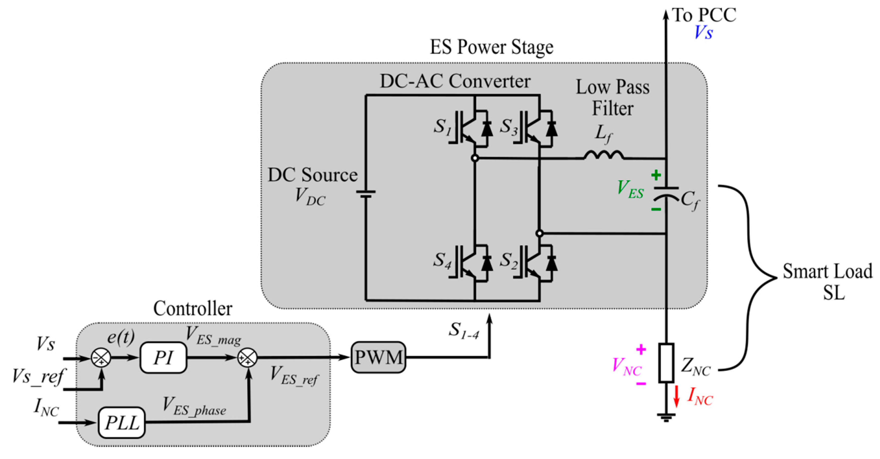
2.1. ES Time-Domain Model
2.2. ES Frequency-Domain Model
3. Model Obtaining
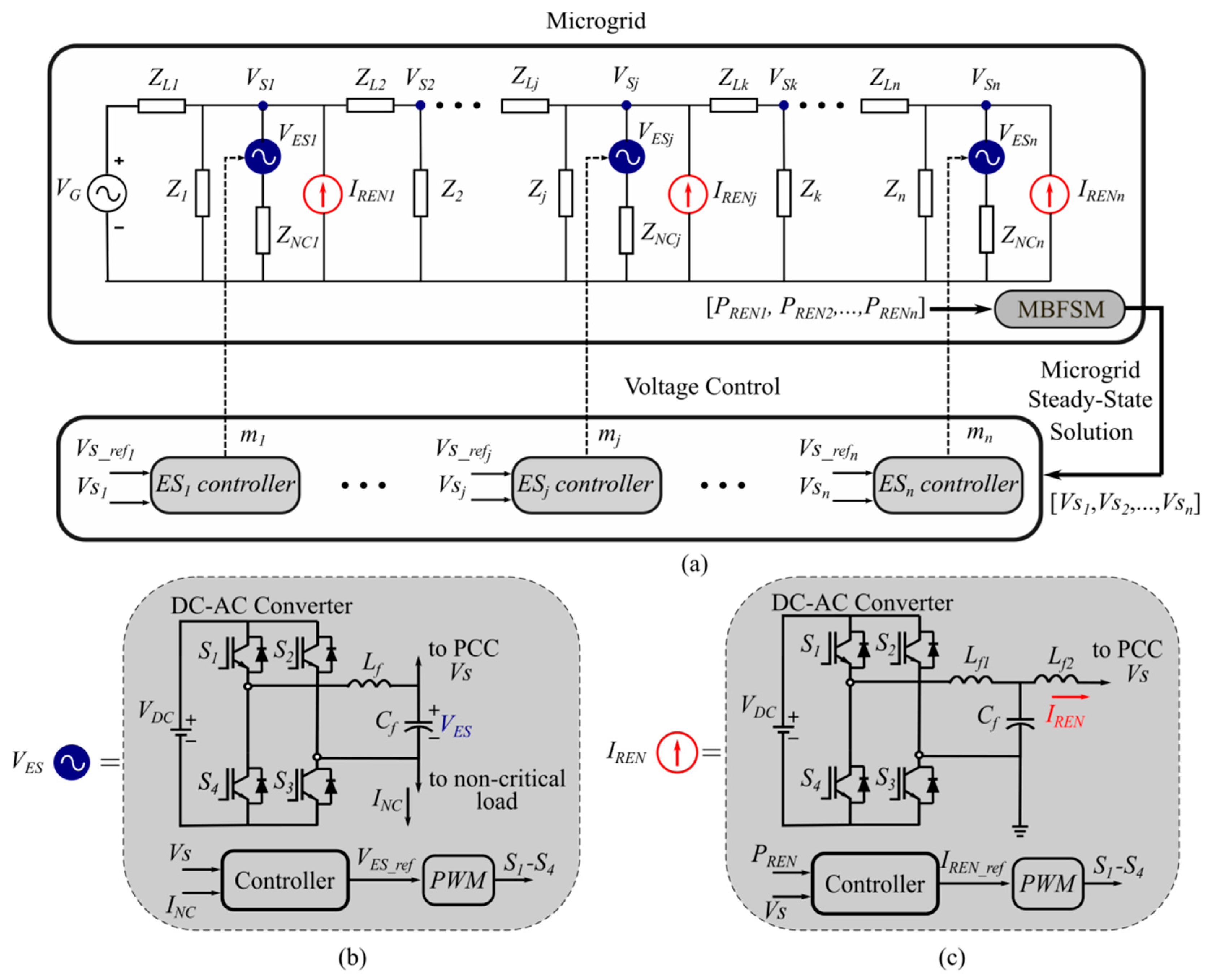
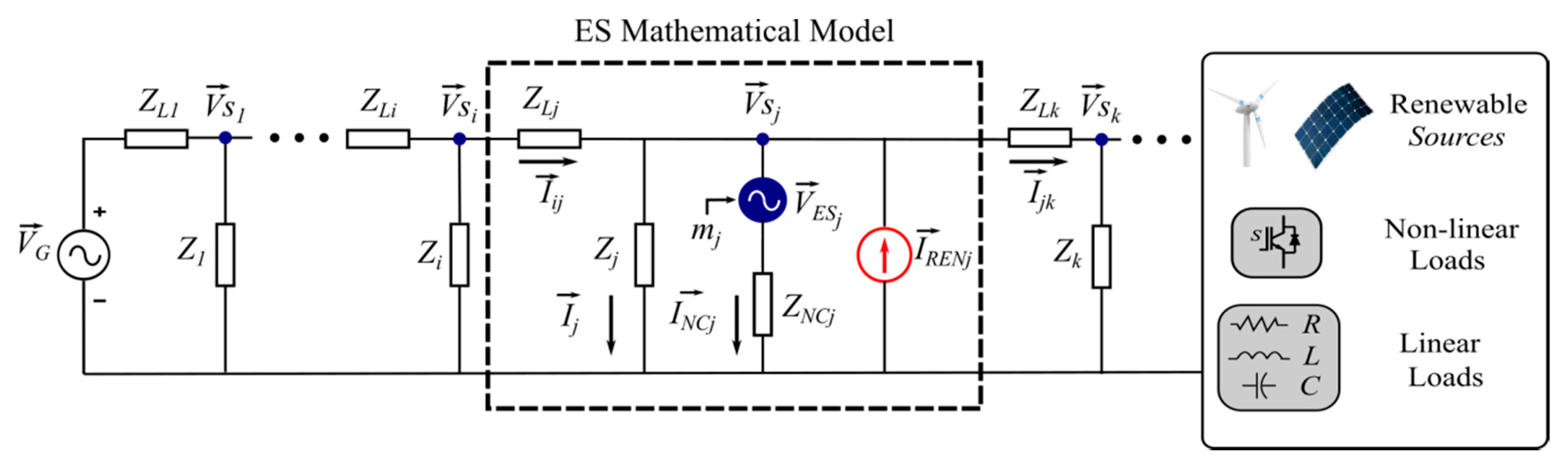
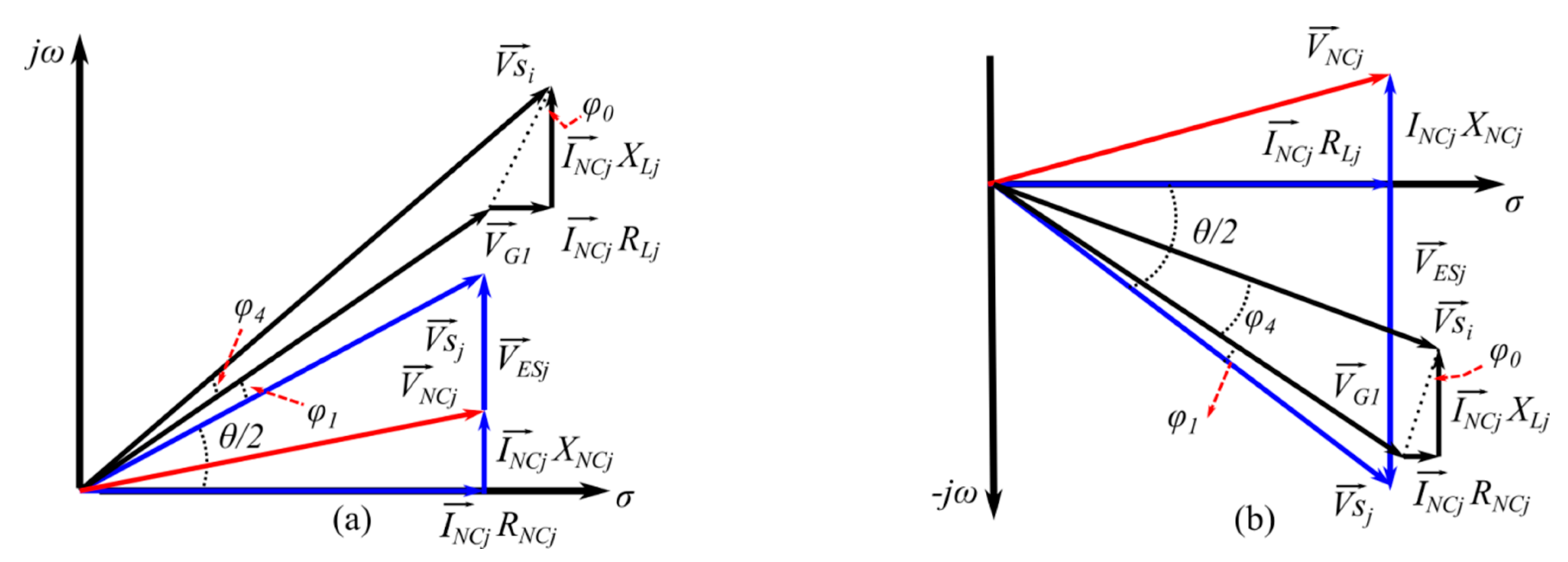
3.1. Steady-State ES Mathematical Model
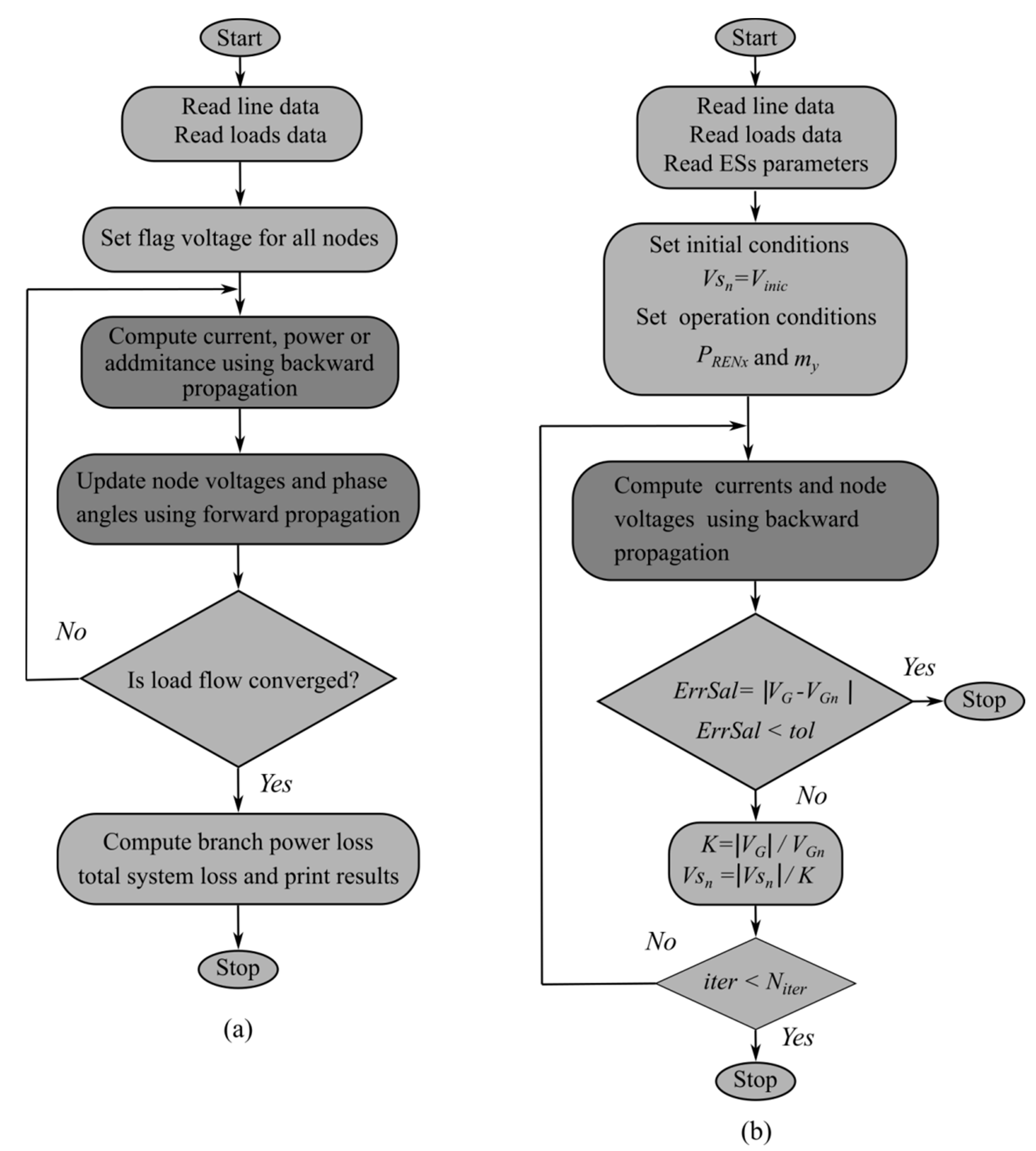
3.2. Modified Backward–Forward Sweep Method
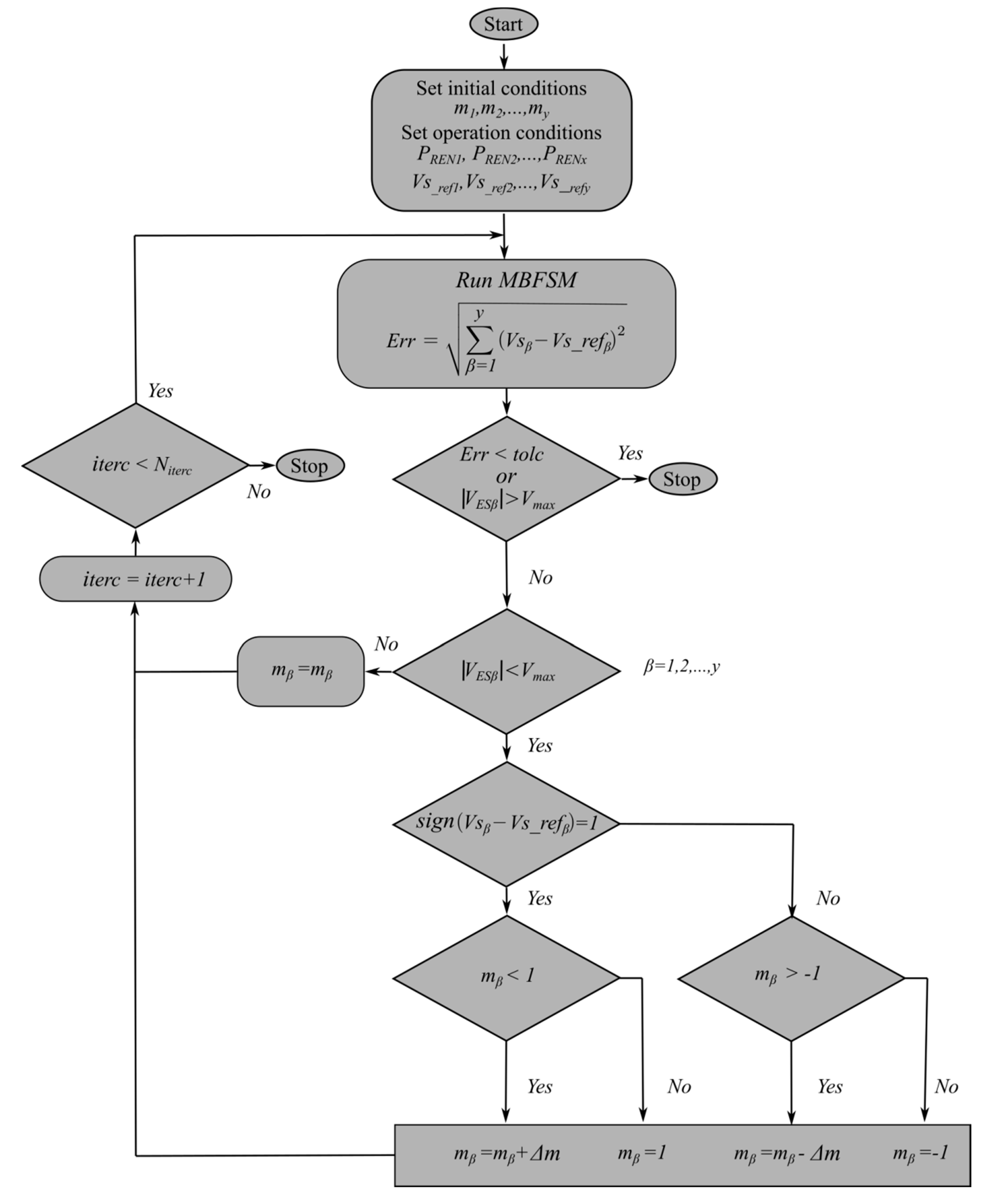
3.3. Voltage Control Algorithm Applied to Multiple ESs
4. Study Cases and Results
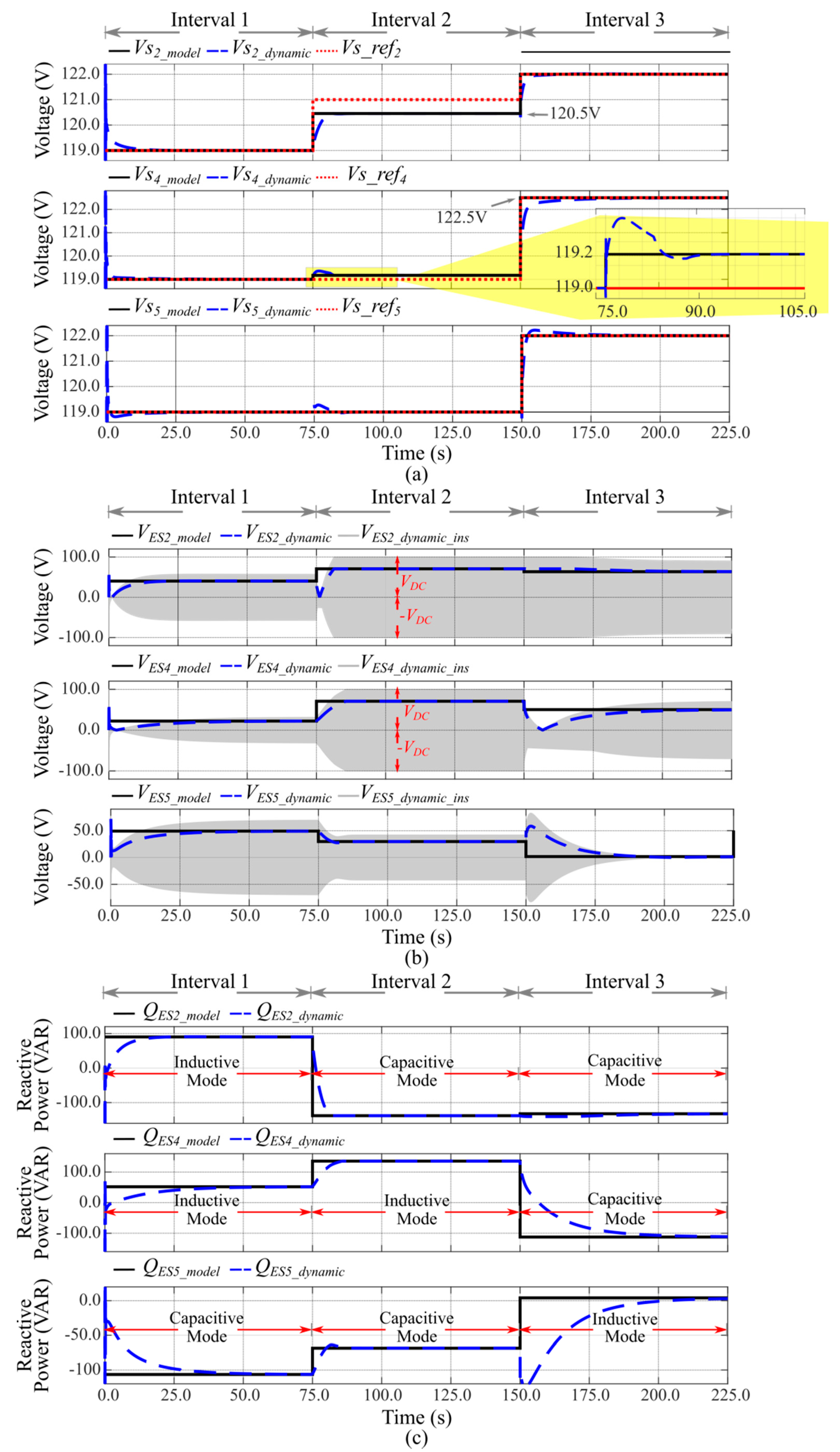
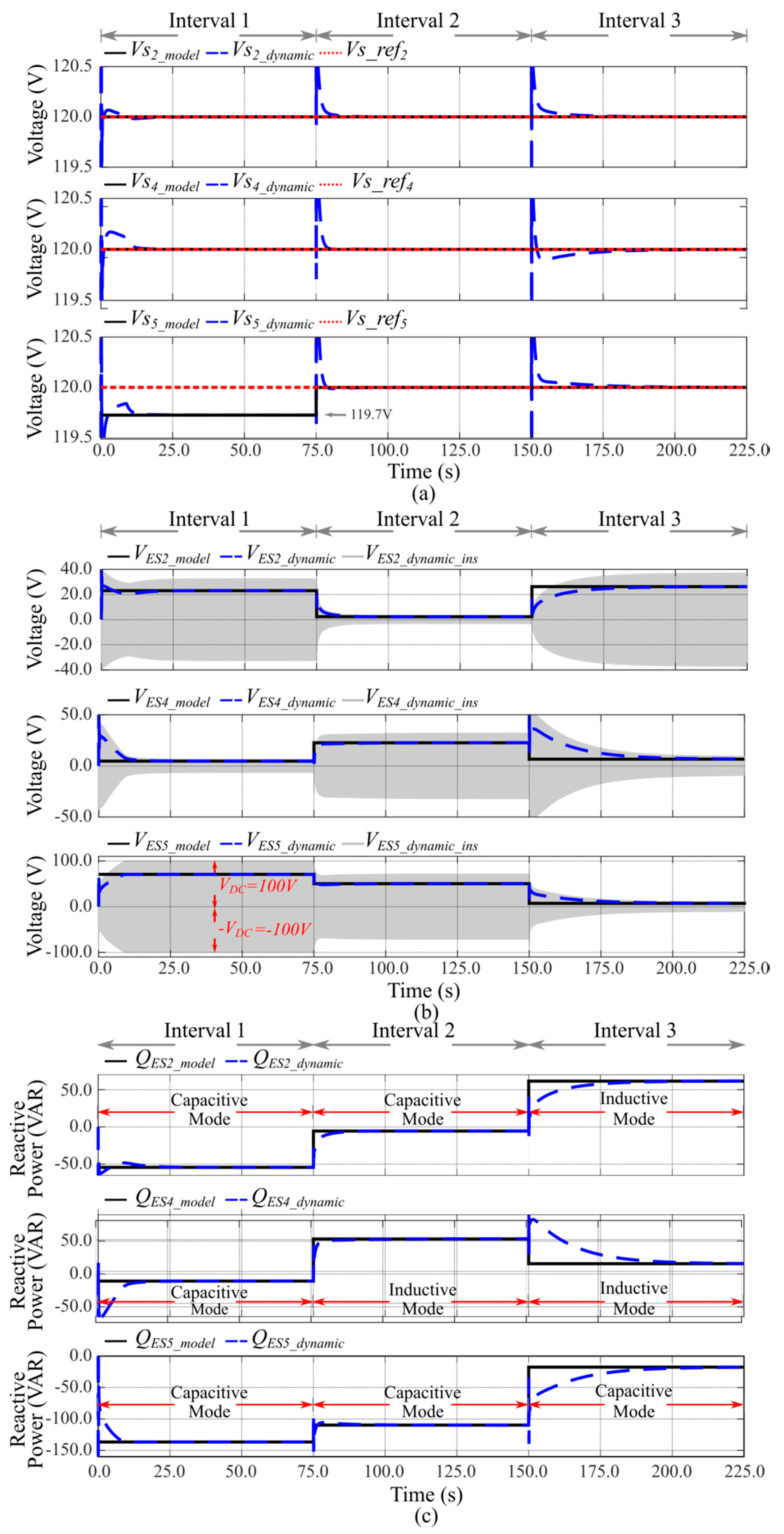
4.1. Study Case: Constant Active Power and Changes in Reference Voltages
4.2. Study Case: Constant Reference Voltages and Changes in ACTIVE POwer
4.3. Quasi-Stationary Simulation Model with Distributed Renewable Generation
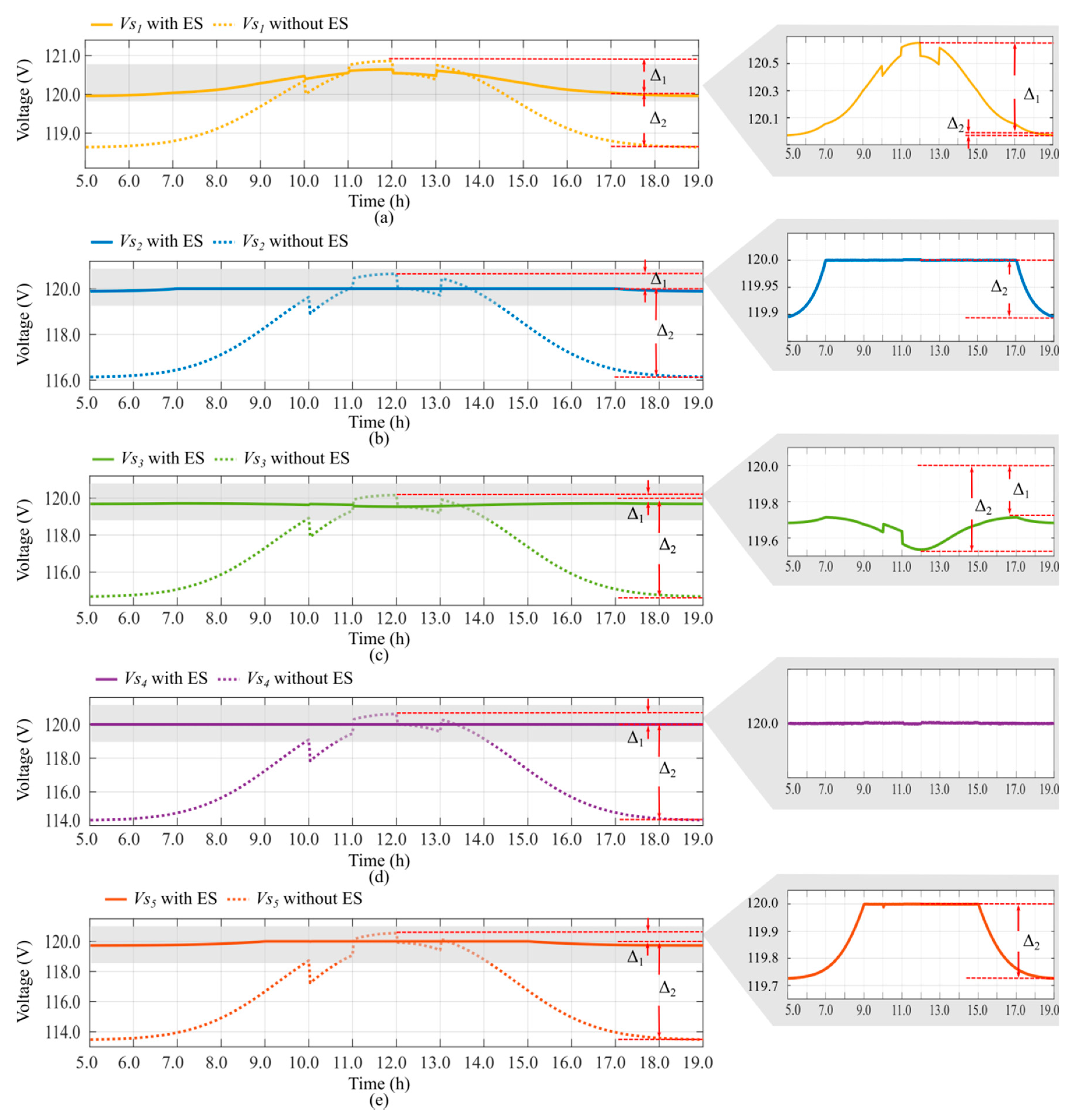
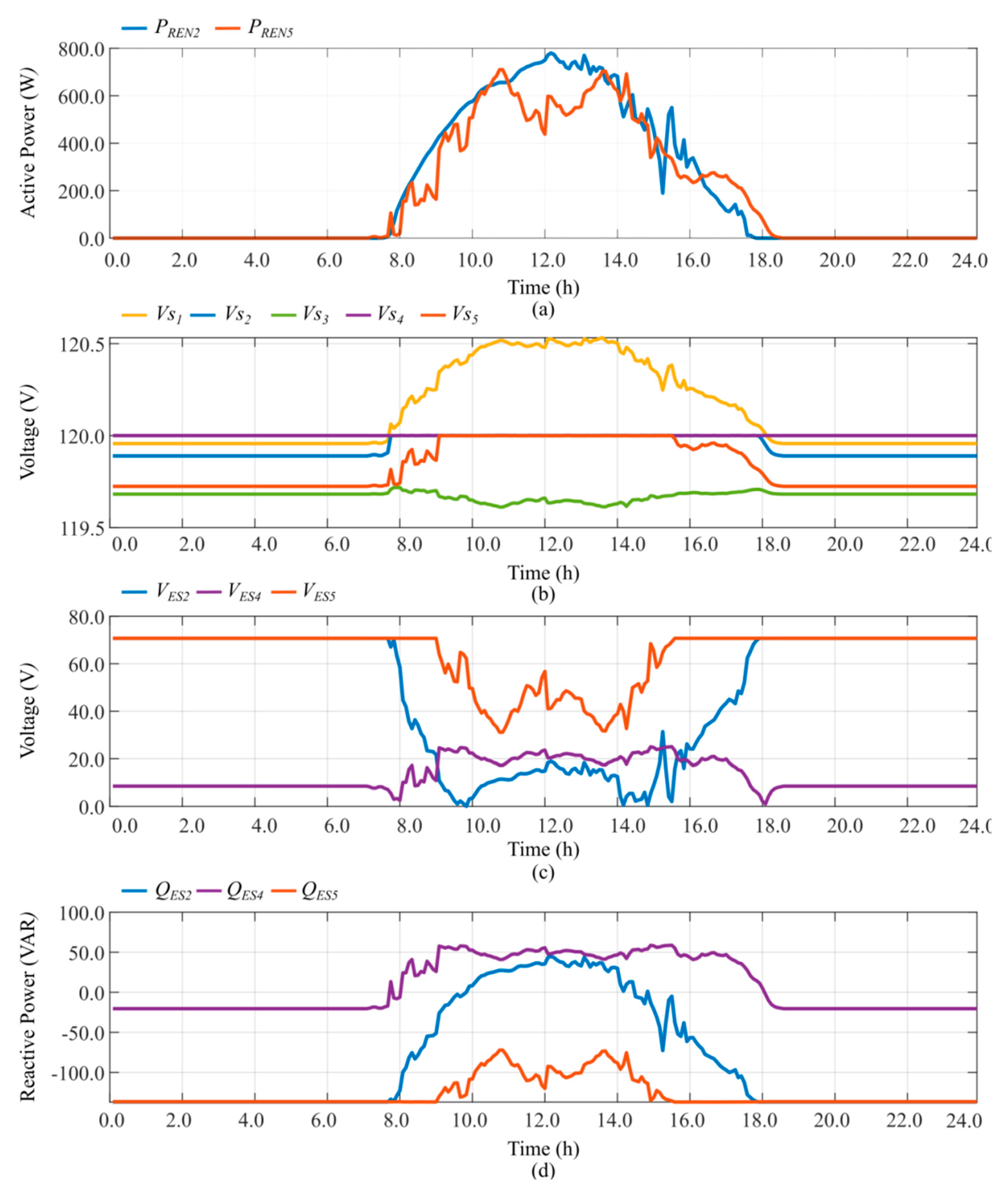
4.4. Quasi-Stationary Simulation Model with Real Power Profiles Data
5. Comparative Analysis of Analytical Models for the ES Applied in Electrical Systems
- The first group is represented by power equations that describe the power exchange of the ES in the PCC; however, they have the constraint of being obtained from a simplified electrical network, indicating that their complexity in the study of multiple ESs will be higher. To adequately describe the behavior of the ESs, the models include additional restrictions related to the characteristics of the network, the physical location of the ES, and their operating limits [24,25,40]. Other alternatives carried out increase the complexity of the model since they include a more significant number of equations [21] or the design of external algorithms that restrict the operation of the ESs within established regions [41,42,43].
- The second group is called phasor models, and within this group is the proposed work. These models are characterized by providing a detailed representation of the geometric relationships of the electrical variables. Although some works have shown its use in grid-connected µGs by considering only one ES [22,23], the needs of modern power systems require the development of more robust models. In this regard, the proposed work outperforms previous works since it can deal with both grid-connected μGs and standalone μGs by considering single and multiple ESs. On the other hand, unlike reported works that consider simplified electrical networks, the proposed model is obtained from a more realistic electrical network by considering the injection of active power into the PCC and the effect of external disturbances on the behavior of the ES. These considerations increase its robustness, allowing for the obtaining of a generalized model suitable for the operation of multiple ESs without the need for additional restrictions. Consequently, a handy tool is obtained to study the requirements of modern energy networks.
6. Conclusions
Author Contributions
Funding
Conflicts of Interest
Nomenclature
| ES | Electric Spring | ϕNC | Non-critical Load Angle |
| SG | Smart Grids | VES | Electric Spring Voltage |
| DG | Distributed Generation | Vs | Voltage on the PCC |
| RES | Renewable Energy Sources | VNC | Non-critical Load Voltage |
| µG | Microgrid | Vs_ref | Reference Voltage on the PCC |
| SL | Smart Load | VES_mag | Magnitude of the ES voltage control |
| PCC | Point of Common Coupling | VES_phase | Phase Angle of the ES Voltage Control |
| DC | Direct Current | VES_ref | ES Voltage Control |
| AC | Alternating Current | INC | Non-critical Load Current |
| BFSM | Backward–forward Solution Method | Voltage Source Phasor | |
| MBFSM | Modified Backward–forward Solution Method | Electric Spring Voltage Phasor | |
| PWM | Pulse Width Modulation | Voltage on the PCC Phasor | |
| PI | Proportional Integral Controller | Non-critical Load Voltage Phasor | |
| R | Resistance | Non-critical Load Current Phasor | |
| L | Inductance | QES | ES Reactive Power |
| C | Capacitance | QNC | Non-critical Load Reactive Power |
| X | Reactance | QSL | Smart Load Reactive Power |
| Z | Critical Load Impedance | PREN | RES Active Power |
| ZNC | Non-critical Load Impedance | IREN | RES Current |
| ZL | Distribution Line Impedance | m | ES operating condition |
References
- Tuballa, M.L.; Abundo, M.L. A review of the development of Smart Grid technologies. Renew. Sustain. Energy Rev. 2016, 59, 710–725. [Google Scholar] [CrossRef]
- Farmanbar, M.; Parham, K.; Arild, Ø.; Rong, C.A. Widespread review of smart grids towards smart cities. Energies 2019, 12, 4484. [Google Scholar] [CrossRef]
- Hossain, M.; Madlool, N.; Rahim, N.; Selvaraj, J.; Pandey, A.; Khan, A.F. Role of smart grid in renewable energy: An overview. Renew. Sustain. Energy Rev. 2016, 60, 1168–1184. [Google Scholar] [CrossRef]
- Zhang, X.; Wang, R.; Bao, J. A novel distributed economic model predictive control approach for building air-conditioning systems in microgrids. Mathematics 2018, 6, 60. [Google Scholar] [CrossRef]
- Yoldaş, Y.; Önen, A.; Muyeen, S.M.; Vasilakos, A.V.; Alan, I. Enhancing smart grid with microgrids: Challenges and opportunities. Renew. Sustain. Energy Rev. 2017, 72, 205–214. [Google Scholar] [CrossRef]
- Jung, S.; Yoon, Y.T.; Huh, J.H. An efficient micro grid optimization theory. Mathematics 2020, 8, 560. [Google Scholar] [CrossRef]
- Fang, W.; Liu, H.; Chen, F.; Zheng, H.; Hua, G.; He, W. DG planning in stand-alone microgrid considering stochastic characteristic. J. Eng. 2017, 2017, 1181–1185. [Google Scholar] [CrossRef]
- Bizon, N.; Thounthong, P. Energy efficiency and fuel economy of a fuel cell/renewable energy sources hybrid power system with the load-following control of the fueling regulators. Mathematics 2020, 8, 151. [Google Scholar] [CrossRef]
- Babazadeh, M.; Nobakhti, A. robust decomposition and structured control of an islanded multi-DG microgrid. IEEE Trans. Smart Grid 2018, 10, 2463–2474. [Google Scholar] [CrossRef]
- Aderibole, A.; Zeineldin, H.H.; Al Hosani, M.; El-Saadany, E.F. Demand side management strategy for droop-based autonomous microgrids through voltage reduction. IEEE Trans. Energy Convers. 2019, 34, 878–888. [Google Scholar] [CrossRef]
- Hui, S.Y.; Lee, C.K.; Wu, F.F. Electric springs—A New smart grid technology. IEEE Trans. Smart Grid 2012, 3, 1552–1561. [Google Scholar] [CrossRef]
- Chen, X.; Hou, Y.; Hui, S.Y.R. Distributed control of multiple electric springs for voltage control in microgrid. IEEE Trans. Smart Grid 2016, 8, 1350–1359. [Google Scholar] [CrossRef]
- Chen, J.; Yan, S.; Yang, T.; Tan, S.C.; Hui, S.Y.R.; Hui, R. Practical evaluation of droop and consensus control of distributed electric springs for both voltage and frequency regulation in microgrid. IEEE Trans. Power Electron. 2018, 34, 6947–6959. [Google Scholar] [CrossRef]
- Chen, J.; Yan, S.; Hui, S.Y.R. Using consensus control for reactive power sharing of distributed Electric Springs. In Proceedings of the 2017 IEEE Energy Conversion Congress and Exposition in Cincinnati, Cincinnati, OH, USA, 1–5 October 2017; pp. 3741–3746. [Google Scholar]
- Akhtar, Z.; Chaudhuri, B.; Hui, S.Y.R. Primary frequency control contribution from smart loads using reactive compensation. IEEE Trans. Smart Grid 2015, 6, 2356–2365. [Google Scholar] [CrossRef]
- Chakravorty, D.; Chaudhuri, B.; Hui, S.Y.R. Rapid Frequency response from smart loads in great britain power system. IEEE Trans. Smart Grid 2017, 8, 2160–2169. [Google Scholar] [CrossRef]
- Zheng, Y.; Hill, D.J.; Song, Y.; Zhao, J.; Hui, S.Y.R. Optimal electric spring allocation for risk-limiting voltage regulation in distribution systems. IEEE Trans. Power Syst. 2020, 35, 273–283. [Google Scholar] [CrossRef]
- Moghbel, M.; Masoum, M.A.S.; Fereidouni, A.; Deilami, S. Optimal sizing, siting and operation of custom power devices with STATCOM and APLC functions for real-time reactive power and network voltage quality control of smart grid. IEEE Trans. Smart Grid 2017, 9, 5564–5575. [Google Scholar] [CrossRef]
- Yang, T.; Liu, T.; Chen, J.; Yan, S.; Hui, S.Y.R.; Hui, R. Dynamic modular modeling of smart loads associated with electric springs and control. IEEE Trans. Power Electron. 2018, 33, 10071–10085. [Google Scholar] [CrossRef]
- Chaudhuri, N.R.; Lee, C.K.; Chaudhuri, B.; Hui, S.Y.R. Dynamic modeling of electric springs. IEEE Trans. Smart Grid 2014, 5, 2450–2458. [Google Scholar] [CrossRef]
- Tan, S.C.; Lee, C.K.; Hui, S.Y. General steady-state analysis and control principle of electric springs with active and reactive power compensations. IEEE Trans. Power Electron. 2012, 28, 3958–3969. [Google Scholar] [CrossRef]
- Zou, Y.; Chen, M.Z.Q.; Hu, Y. Steady-state analysis and output voltage minimization based control strategy for electric springs in the smart grid with multiple renewable energy sources. Complexity 2019, 2019, 1–12. [Google Scholar] [CrossRef]
- Wang, Q.; Cheng, M.; Chen, Z.; Wang, Z. Steady-state analysis of electric springs with a novel δ control. IEEE Trans. Power Electron. 2015, 30, 7159–7169. [Google Scholar] [CrossRef]
- Akhtar, Z.; Chaudhuri, B.; Hui, S.Y.R. Smart loads for voltage control in distribution networks. IEEE Trans. Smart Grid 2015, 8, 1–10. [Google Scholar] [CrossRef]
- Askarpour, M.; Aghaei, J.; Boudjadar, J.; Niknam, T. Techno-economic potential gains of electric springs in distribution networks operations. IET Gener. Transm. Distrib. 2020, 14, 98–107. [Google Scholar] [CrossRef]
- Khamis, A.K.; Zakzouk, N.E.; Abdelsalam, A.K.; Lotfy, A.A. Decoupled control strategy for electric springs: Dual functionality feature. IEEE Access 2019, 7, 57725–57740. [Google Scholar] [CrossRef]
- Wang, M.-H.; Yang, T.; Tan, S.C.; Hui, S.Y.R.; Hui, R. Hybrid electric springs for grid-tied power control and storage reduction in AC microgrids. IEEE Trans. Power Electron. 2018, 34, 3214–3225. [Google Scholar] [CrossRef]
- Mok, K.-T.; Wang, M.-H.; Tan, S.C.; Hui, S.Y.R. DC Electric springs—A Technology for stabilizing DC power distribution systems. IEEE Trans. Power Electron. 2016, 32, 1088–1105. [Google Scholar] [CrossRef]
- Lee, C.K.; Chaudhuri, B.; Hui, S.Y. Hardware and control implementation of electric springs for stabilizing future smart grid with intermittent renewable energy sources. IEEE J. Emerg. Sel. Top. Power Electron. 2013, 1, 18–27. [Google Scholar] [CrossRef]
- Sen, B.; Soni, J.; Panda, S.K. Performance of electric springs with multiple variable loads. In Proceedings of the 2016 IEEE 8th International Power Electronics and Motion Control Conference (IPEMC-ECCE Asia), Hefei, China, 22–26 May 2016; Institute of Electrical and Electronics Engineers (IEEE-USA): Riverside, CA, USA, 2016; pp. 3290–3295. [Google Scholar]
- Luo, X.; Akhtar, Z.; Lee, C.K.; Chaudhuri, B.; Tan, S.C.; Hui, S.Y.R. Distributed voltage control with electric springs: Comparison with STATCOM. IEEE Trans. Smart Grid 2014, 6, 209–219. [Google Scholar] [CrossRef]
- Ganesh, J.A.M.R.; Power, S. flow analysis for radial distribution system using backward/forward sweep method. Int. J. Electr. Comput. Eng. 2014, 8, 1628–1632. [Google Scholar]
- Lee, C.K.; Chaudhuri, N.R.; Chaudhuri, B.; Hui, S.Y.R. Droop control of distributed electric springs for stabilizing future power grid. IEEE Trans. Smart Grid 2013, 4, 1558–1566. [Google Scholar] [CrossRef]
- Thukaram, D.; Banda, H.W.; Jerome, J. A robust three phase power flow algorithm for radial distribution systems. Electr. Power Syst. Res. 1999, 50, 227–236. [Google Scholar] [CrossRef]
- NREL. Available online: https://www.nrel.gov/grid/solar-power-data.html (accessed on 20 July 2020).
- Sharma, S.K.; Chandra, A.; Saad, M.; Lefebvre, S.; Asber, D.; Lenoir, L. Voltage flicker mitigation employing smart loads with high penetration of renewable energy in distribution systems. IEEE Trans. Sustain. Energy 2017, 8, 414–424. [Google Scholar] [CrossRef]
- Wang, Q.; Cheng, M.; Jiang, Y. Harmonics suppression for critical loads using electric springs with current-source inverters. IEEE J. Emerg. Sel. Top. Power Electron. 2016, 4, 1362–1369. [Google Scholar] [CrossRef]
- Yang, Y.; Qin, Y.; Tan, S.; Hui, S.Y.R. Reducing distribution power loss of islanded AC microgrids using distributed electric springs with predictive control. IEEE Trans. Ind. Electron. 2020, 67, 9001–9011. [Google Scholar] [CrossRef]
- Pandey, A.; Pileggi, L. Steady-state simulation for combined transmission and distribution systems. IEEE Trans. Smart Grid 2020, 11, 1124–1135. [Google Scholar] [CrossRef]
- Liang, L.; Hou, Y.; Hill, D.J. Enhancing flexibility of an islanded microgrid with electric springs. IEEE Trans. Smart Grid 2017, 10, 899–909. [Google Scholar] [CrossRef]
- Liang, L.; Hou, Y.; Hill, D.J.; Hui, S.Y.R. Enhancing resilience of microgrids with electric springs. IEEE Trans. Smart Grid 2016, 9, 2235–2247. [Google Scholar] [CrossRef]
- Norouzi, M.; Aghaei, J.; Pirouzi, S.; Niknam, T.; Lehtonen, M. Flexible operation of grid-connected microgrid using ES. IET Gener. Transm. Distrib. 2020, 14, 254–264. [Google Scholar] [CrossRef]
- Liang, L.; Hou, Y.; Hill, D.J. An interconnected microgrids-based transactive energy system with multiple electric springs. IEEE Trans. Smart Grid 2020, 11, 184–193. [Google Scholar] [CrossRef]


| Distribution Lines | Loads | Non-Critical Loads | DC Bus for ESs | ||||||
|---|---|---|---|---|---|---|---|---|---|
| Element | Resistance (Ω) | Reactance (Ω) | Element | Resistance (Ω) | Reactance (Ω) | Element | Resistance (Ω) | Element | Voltage (V) |
| ZL1 | 0.1 | 0.4599 | Z1 | 0 | −70 | ZNC2 | 50 | VDC2 | 100 |
| ZL2 | 0.1 | 0.9048 | Z2 | 53 | 0 | ZNC4 | 50 | VDC4 | 100 |
| ZL3 | 0.1 | 0.9048 | Z3 | 53 | 50 | ZNC5 | 50 | VDC5 | 100 |
| ZL4 | 0.1 | 0.4599 | Z4 | 0 | −70 | ||||
| ZL5 | 0.1 | 0.4599 | Z5 | 53 | 50 | ||||
| Sampling Time | Proportional Gain (Kp) | Integral Gain (Ki) | Integral Gain (Kd) | |
|---|---|---|---|---|
| PI Controllers | 0.0167 s | 10 | 30 | |
| PLL | 0.001 s | 180 | 3200 | 1 |
| BFSM Iterations | MBFSM Iterations | Reduction of Average Iterations (%) | |||||
|---|---|---|---|---|---|---|---|
| err | Max | Min | Average | Max | Min | Average | |
| 1 × 10⁻¹ | 5 | 3 | 4 | 3 | 1 | 3 | 25.0 |
| 1 × 10⁻² | 7 | 3 | 5 | 4 | 2 | 3 | 40.0 |
| 1 × 10⁻³ | 9 | 3 | 6 | 5 | 2 | 4 | 33.3 |
| 1 × 10⁻⁴ | 10 | 4 | 8 | 6 | 3 | 5 | 37.5 |
| 1 × 10⁻⁵ | 12 | 5 | 9 | 7 | 3 | 6 | 33.3 |
| 1 × 10⁻⁶ | 14 | 5 | 10 | 7 | 4 | 6 | 40.0 |
| 1 × 10⁻¹² | 21 | 9 | 17 | 12 | 7 | 11 | 35.2 |
| Average | 34.9 | ||||||
| Without Control | With Control | Improvement on the Voltage Eduction (%) | ||||
|---|---|---|---|---|---|---|
| Voltages | Δ1 | Δ2 | Δ1 | Δ2 | Δ1 | Δ2 |
| Vs1 | −0.8604 V | 1.3681 V | −0.6423 V | 0.0427 V | NA | NA |
| Vs2 | −0.6533 V | 3.8775 V | 0 V | 0.1098 V | 100 | 97.1683 |
| Vs3 | −0.1660 V | 5.3455 V | 0.2848 V | 0.4661 V | NA | NA |
| Vs4 | −0.6166 V | 5.7038 V | 0 V | 0 V | 100 | 100 |
| Vs5 | −0.5413 V | 6.5444 V | 0 V | 0.2758 V | 100 | 95.7857 |
| Mathematical Model | ||||
|---|---|---|---|---|
| Dynamic | Steady-State | |||
| Power Equations | Phasor | |||
| References | [15,26,36,37,38] | [21,24,25,39,40,41,42,43] | [22,23] | This work |
| Type of electric system |
|
| • Grid-connected µGs |
|
| ESs |
|
| • Single |
|
| RES | Yes | Yes | No | Yes |
| Require equivalent power system circuits | No | Yes | Yes | No |
| Computational effort | High | Low | Low | Low |
| Additional constraints | No | Yes | No | No |
| Attributes |
| |||
| • The calculation of geometric relationships has been limited to simplified electrical networks |
| |||
© 2020 by the authors. Licensee MDPI, Basel, Switzerland. This article is an open access article distributed under the terms and conditions of the Creative Commons Attribution (CC BY) license (http://creativecommons.org/licenses/by/4.0/).
Share and Cite
Tapia-Tinoco, G.; Granados-Lieberman, D.; Rodriguez-Alejandro, D.A.; Valtierra-Rodriguez, M.; Garcia-Perez, A. A Robust Electric Spring Model and Modified Backward Forward Solution Method for Microgrids with Distributed Generation. Mathematics 2020, 8, 1326. https://doi.org/10.3390/math8081326
Tapia-Tinoco G, Granados-Lieberman D, Rodriguez-Alejandro DA, Valtierra-Rodriguez M, Garcia-Perez A. A Robust Electric Spring Model and Modified Backward Forward Solution Method for Microgrids with Distributed Generation. Mathematics. 2020; 8(8):1326. https://doi.org/10.3390/math8081326
Chicago/Turabian StyleTapia-Tinoco, Guillermo, David Granados-Lieberman, David A. Rodriguez-Alejandro, Martin Valtierra-Rodriguez, and Arturo Garcia-Perez. 2020. "A Robust Electric Spring Model and Modified Backward Forward Solution Method for Microgrids with Distributed Generation" Mathematics 8, no. 8: 1326. https://doi.org/10.3390/math8081326
APA StyleTapia-Tinoco, G., Granados-Lieberman, D., Rodriguez-Alejandro, D. A., Valtierra-Rodriguez, M., & Garcia-Perez, A. (2020). A Robust Electric Spring Model and Modified Backward Forward Solution Method for Microgrids with Distributed Generation. Mathematics, 8(8), 1326. https://doi.org/10.3390/math8081326