1. Introduction
In 1931, to study the relationship between the growth of a species and its density, Allee [
1] proposed the effect later called the Allee effect, which means that the population size will decrease if it is too sparse. The Allee effect occurs due to lots of factors, including inbreeding, depression [
2], difficulty in finding spouses [
3], social dysfunction at low-densities [
4], and so on. In the following, we mention two single species models with Allee effects.
The first one proposed by Bazykin [
5] is described by the following equation.
where
r denotes the intrinsic per capita growth rate of the population and
K is the carrying capacity of the environment. Model (1) is said to havecq strong Allee effect if
and to have a weak Alleee effect if
. To study the dynamics, Bazykin introduced a population threshold, which is the minimum population size for the species to survive. It is shown that with a strong Allee effect, the population must surpass this threshold in order to grow. However, there is no threshold for a weak effect.
Further, in a study on how mating affects a population’s reproductive rate, Dennis [
6] found that not only can a lack of mates affect it, but also the mating function has a great influence on the birth rate in the population growth rate. To describe the Allee effect of prey, the isometric hyperbolic function is used. Under such circumstances, the Allee effect is called additive. The single species model with an additive Allee effect proposed in [
6] is as follows.
where
m and
a are constants, which reflect the degree of Allee effect. Biologically,
m denotes the rate for level of Allee effect and
a represents the population size of the prey specie whose fitness is half its maximum value. Note that if
then (2) has the weak Allee effect and if
then it has the strong Allee effect. For sparse populations experiencing the Allee effect, Dennis demonstrated with numerical simulations that the critical density, the growth, and the extinction probability can be obtained. Until now, many researchers have paid a great deal of attention on the impact of Allee effect on predation (see [
7,
8,
9,
10,
11,
12,
13,
14,
15,
16,
17,
18]). For example, Liu et al. [
9] showed that a system with gestation delay and an additive Allee effect is unstable if economic interest increases through zero, which may occur in the case of an Allee effect (strong or weak). In [
10], they found the extinction of species due to the Allee effect.
Research has indicated that predators can not only kill prey directly but also affect the behavior of prey, and the latter is more lethal than the former. In fact, all animals show many kinds of anti-predator responses, such as changes of foraging behavior, habitat usage, physiology, and so on ([
19,
20,
21,
22,
23]). To describe that, the concept of fear in the prey was introduced and studied ([
24,
25,
26,
27,
28,
29,
30]). In particular, Wang et al. [
29] for the first time proposed the following predator–prey model with the cost of fear:
where
k is the level of fear, which is due to anti-predator behaviors of the prey;
g is the functional response. Based on the biological background, the following reasonable assumptions are imposed,
Taking the linear functional response, i.e.,
, Wang et al. found that if
then
is globally asymptotically stable and if
then the unique positive equilibrium
is globally asymptotically stable. Moreover, analysis reveals that the fear factor does not change the stability of the equilibrium when it exists. In (3), the fear factor affects the intrinsic growth rate. Then, inspired by [
29] Sasmal [
30] considered the case wherein the fear factor impacts the growth rate and the growth rate has the strong Allee effect. The model studied is given by
where
f represents the effect of fear. It was found that (4) undergoes a subcritical Hopf-bifurcation at
. Moreover, changing the parameter values of
and
m can produce bi-stability or stable oscillatory coexistence of both prey and predator. It was further observed that the change of
f can only change the density of predator at the positive equilibrium but not the stability of the equilibrium.
To the best of our knowledge, so far there is not much being done on predator–prey models with both the additive Allee effect and the fear effect. This motivated us to modify (4) by replacing the Allee effect with the additive Allee effect. Precisely, we studied the following model:
where
and
stand for the fear effect and additive Allee effect, respectively;
r is the intrinsic growth rate of prey;
b is the predation rate;
is the conversion coefficient; and
n is the death rate of the predator. As we known, the relationship between prey and predator has always been the focus of scholars [
31,
32,
33,
34,
35,
36,
37]; hence, this paper will enrich the literature in this field.
The remaining part of this paper is organized as follows. First, we study the existence and local stability of equilibria of (5) in
Section 2 and
Section 3, respectively. Then we provide sufficient conditions ensuring the global stability of the positive equilibrium in
Section 4. In
Section 5 is the bifurcation analysis, which includes saddle-node bifurcation, transcritical bifurcation, and Hopf bifurcation. These theoretical results are supported with numerical simulations in
Section 6. The paper concludes with a discussion on the impact of the fear effect.
2. Existence of Equilibria
Obviously, system (5) always has the trivial equilibrium
. In order to obtain the other equilibria, we consider the two nullclines:
Note that if from the second line of (6). Additionally, from this equation, we get (which corresponding to the boundary equilibria) and with (which corresponds to the positive or internal equilibrium).
We first study the existence of boundary equilibria. Substituting
into 1st line of (6) gives
or
Let . Then when and hence (7) only has one root, denoted by ; when and hence it has two roots, denoted by and ; when and hence it has no real roots. Note that and if and only if . Based on the above discussion, we can have the following result on the existence of boundary equilibria.
Lemma 1. The following results on the existence of boundary equilibria of (5) are true.
- (i)
Suppose . Then the existence of boundary equilibria in addition to is summarized in Table 1. - (ii)
Suppose . Then besides , there is also another boundary equilibrium only when .
- (iii)
Suppose . Then besides , there is also another boundary equilibrium only when .
Next, we consider the existence of positive equilibria. In this case, we have
. Substituting it into 1st line of (6) gives
The above equation has positive solutions only when , and in this case it has only one positive solution , where . Additionally, in other cases, there is no positive root. That is summarized in the following result.
Lemma 2. Let . Then (5) has positive equilibria only when , and in this case, there is only one positive equilibrium , where with . Additionally, in other cases, there is no positive equilibrium.
3. Local Stability of Equilibria
The purpose of this section is to study the local stability of the equilibria obtained in Lemmas 1 and 2 one by one. Note that both and are in fact .
Theorem 1. The trivial equilibrium of (5) is a stable node if or , a saddle-node if , and a saddle if .
Proof. The Jacobian matrix of (5) at
is
whose eigenvalues are
and
. If
then
and hence
is a stable node while if
then
is a saddle as
. What left is what happens when
, as in this case
. To study the stability of
, we rescale
t by
and expand the resulting system from (5) in power series up to the third order around
to get
where
is a power series in
with terms
satisfying
. By applying Theorem 7.1 of Chapter 2 in [
38], we see that
is a saddle-node if
as the coefficient of
,
, is not 0; and
is a stable node if
as in this case that coefficient of
is 0 but
. □
Next, we consider .
Theorem 2. The boundary equilibrium of (5) is a saddle-node if , but if then is a saddle.
Proof. The Jacobian matrix at
is given by
where
. Recall that when
exists we have
which implies that
. Thus the one eigenvalues of
is
.
(i) , then the discussion on the stability of is similar to the last part of the proof of Theorem (8).
We first translate
into the origin by the transformation
and expand the resulting system from (5) in power series up to the second order around the origin to get
where
is a power series in
with terms
satisfying
. Now we apply the transformation
and then the rescaling
to transform (8) into the following standard form:
where
is a power series in
with terms
satisfying
. Since the coefficient of
,
is not 0, we know that
is a saddle-node by Theorem 7.1 of Chapter 2 in [
38].
(ii)
and let
; then (8) change into the following form,
Let
; then we have the following implicit functions
and
By Theorems 7.2 and 7.3 and the corollary (see page 120 to 121) of Chapter 2 in [
38], we have
,
;
, and thus
is a saddle. The proof completes.
For the stability of
, we note that the Jacobian matrix at
is
where
. Recall that
exists when
and
. It follows that
As the two eigenvalues of are and , the following result follows immediately. □
Theorem 3. The boundary equilibrium of (5) is always unstable. In particular, is an unstable node if , it is a saddle if , and it is a saddle-node if (this proof is similar to Theorem 1 (i)).
From the previous section, we can see that
exists if
and
;
exists if
and
;
exists if
and
. Now, we study the stability of
(
, 4, 5). The Jacobian matrix at
is
where
for
and 5 and
. The eigenvalues of
are
and
. As in the discussion for
, one can easily show that
by using the conditions guaranteeing its existence. Therefore, the following theorem summarizes the results on stability of
.
Theorem 4. For , 4, and 5, the boundary equilibrium of (5) is a saddle if ; it is a stable node if ; and it is a saddle-node if (this proof is similar to Theorem 1 (i)).
Finally, we consider the stability of the positive equilibrium .
Theorem 5. The positive equilibrium of (5) is locally asymptotically stable if and unstable if .
Proof. The Jacobian matrix of (5) at
is
Note that
from the condition on the existence of
and
It is easy to see that if , if , and if . Therefore, both eigenvalues of have negative real parts if , have positive real parts if , and have zero real parts if . Then the desired result follows. □
5. Bifurcation Analysis
From the local stability analysis, we see that there are bifurcations occurring. In this section, we derive conditions on saddle-node bifurcation, transcritical bifurcation, and Hopf bifurcation.
Firstly, in order to prove the saddle-node bifurcation and transcritical bifurcation of system (5), we need the following Lemma (Sotomayor’s Theorem in [
39,
40]).
Theorem 7 (Sotomayor’s Theorem in [
39,
40]).
Consider the system as follows.Suppose at equilibrium holds. Additionally, assume that the matrix has one characteristic root , and both V and W are eigenvectors belonging to the eigenvalue of the matrix A and , respectively. Then
- (1)
SupposeHence, when the bifurcation parameter μ has a critical value, that is, , system (10) undergoes a saddle-node bifurcation at . - (2)
SupposeHence, when μ is of a critical value, that is, , system (10) undergoes a transcritical bifurcation at .
By
Table 1 of Lemma 2.1, when
, system (5) has two boundary equilibria
and
if
, has one boundary equilibrium
if
, and has no boundary equilibrium if
. This suggests a bifurcation around
. The above analysis indicates that we can choose the parameter
m in the additive Allee effect as the bifurcation parameter to obtain saddle-node bifurcation.
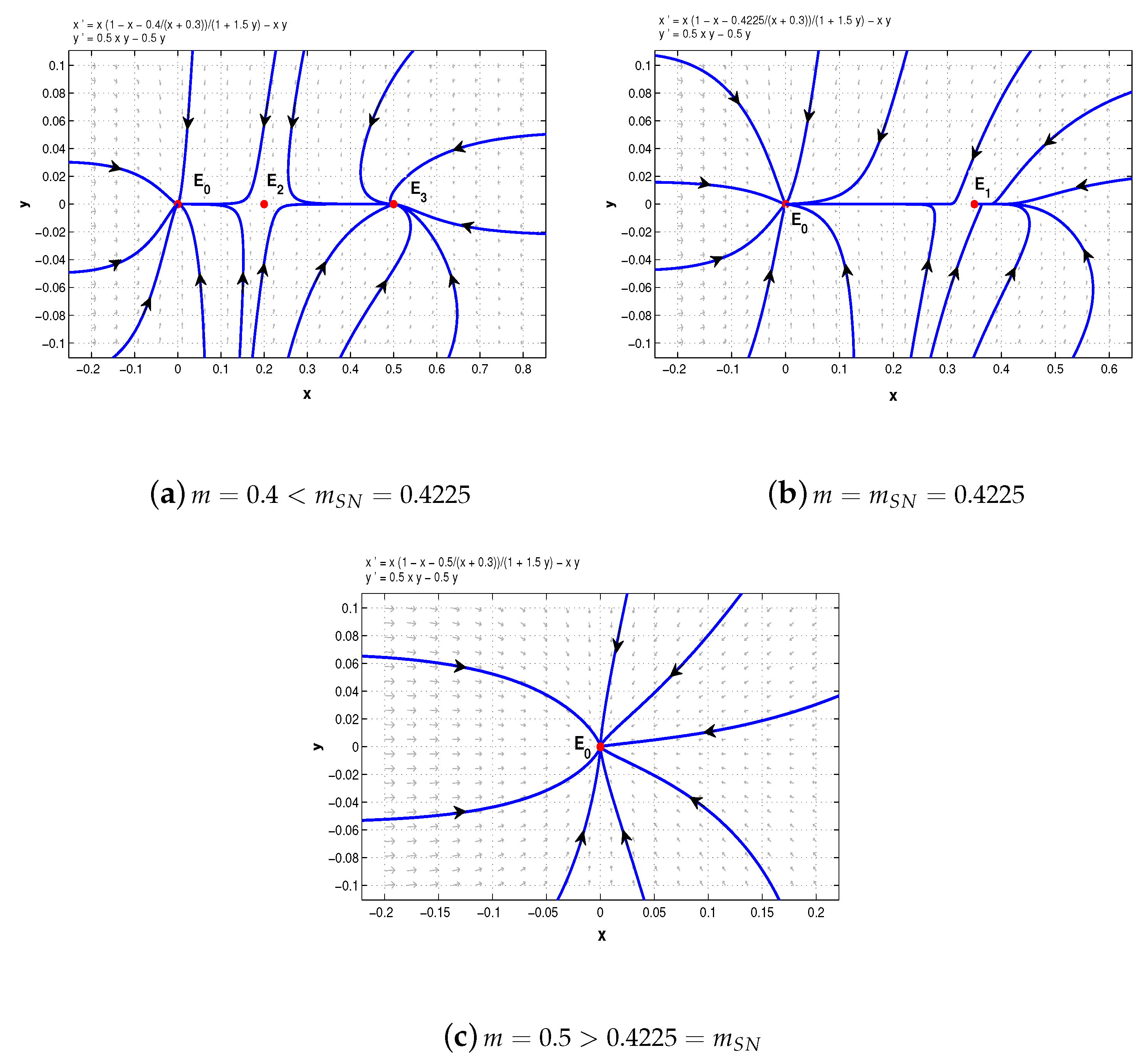
Theorem 8. Suppose and . Then (5) undergoes a saddle-node bifurcation from at .
Proof. When
and
, (5) has the unique boundary equilibrium
. We apply Lemma 3 to study the bifurcation around
. Firstly, we easily see that the Jacobian matrix
has the two eigenvalues
and
. Choose the eigenvectors
V and
W associated with the eigenvalue
of
and
given respectively by
Therefore, system (5) undergoes a saddle-node bifurcation at . □
To illustrate the saddle-node bifurcation, we chose
,
,
,
,
. Then
. When
, system (5) has two distinct boundary equilibria,
and
; when
,
collapses to
and only the boundary equilibrium
remains. However, when
, the boundary equilibrium
also disappears (see
Figure 1).
Next, by
Table 1 of Lemma 2.1, system (5) has two boundary equilibria
and
if
, has one boundary equilibrium
(
and
coincide)if
, and has two boundary equilibria
(
) and
if
. This suggests a bifurcation around
. The above analysis indicates that we can choose the parameter
a as the bifurcation produces transcritical bifurcation.
Theorem 9. Suppose that . Then system (5) undergoes a transcritical bifurcation from at .
Proof. The proof is similar to that of Theorem 7. We just verify the condition on transcritical bifurcation of Lemma 3. When
, we have
whose eigenvalues are
and
. Choose the eigenvectors of
and
associated with the eigenvalue
given respectively by
Let
F be defined as in the proof of Theorem 7. Then
Then we easily see that
V and
W satisfy
Therefore, system (5) undergoes transcritical bifurcation from at .
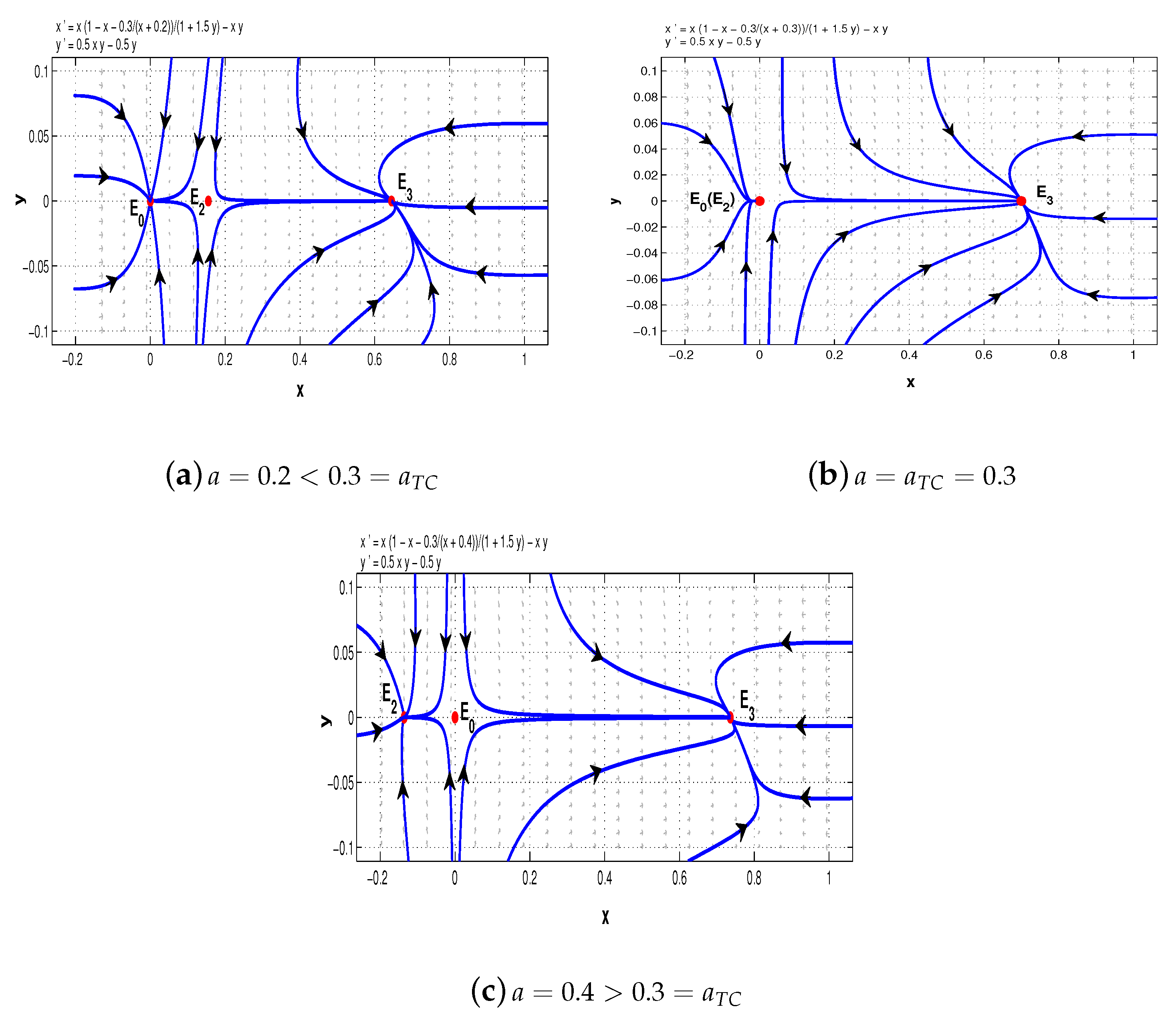
With
,
,
,
,
,
Figure 2 shows the transcritical bifurcation with
,
, and
.
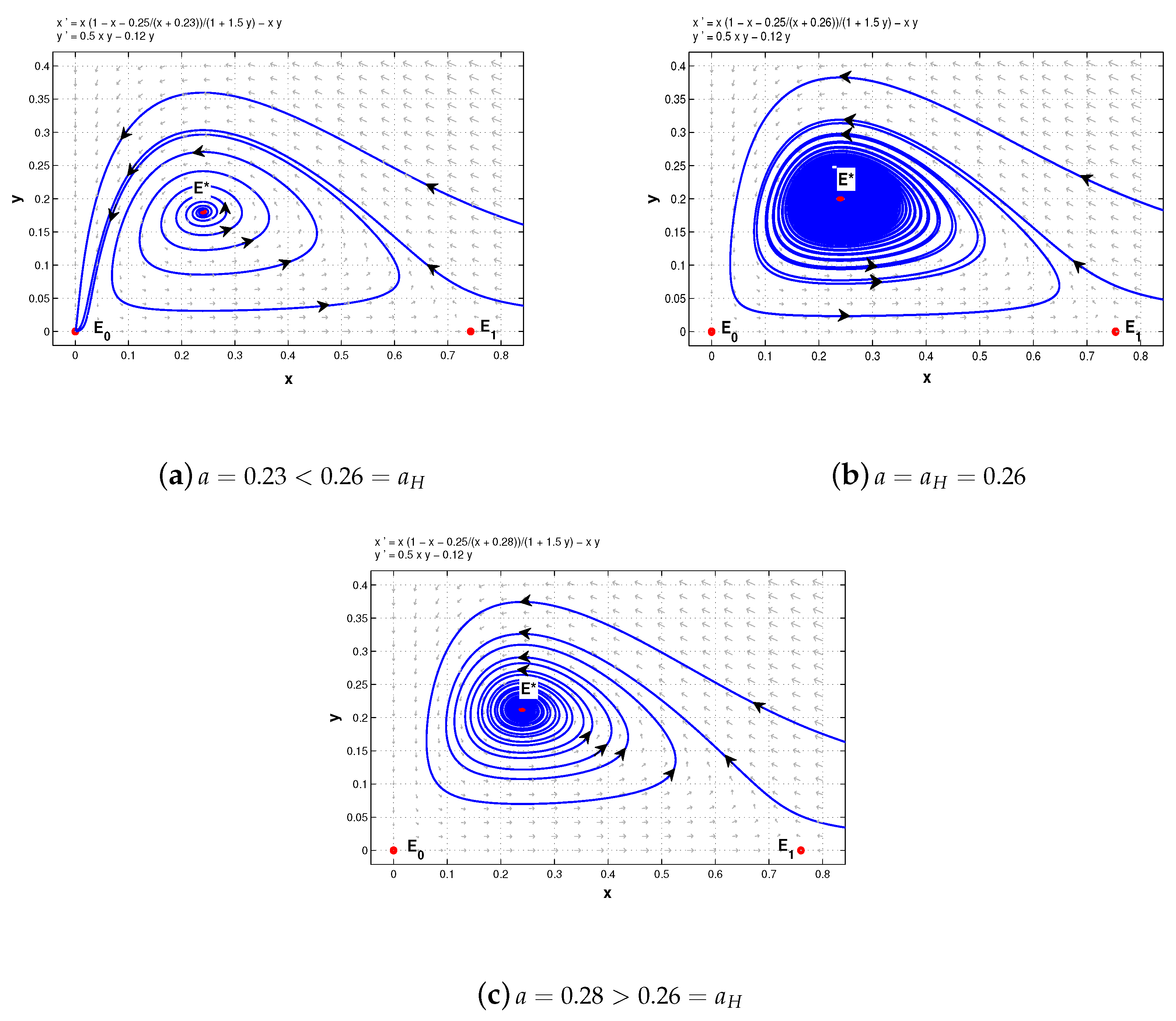
In the remainder of this section, we consider Hopf bifurcation. From Theorem 5 and its proof, it is easily concluded that the positive equilibrium of system (5) is locally asymptotically stable if , is a center if , and through Hopf bifurcation loses its stability under appropriate parameters. In the following we choose a as the bifurcation parameter to show that.
Theorem 10. Under the assumptions on the existence of the positive equilibrium of system (5), that is, , then there is a supercritical Hopf bifurcation from at , where .
Proof. Recall that the characteristic equation of the Jacobian matrix
is
where
Clearly,
is a center when
and
Thus a Hopf bifurcation from occurs at . To discuss the stability (direction) of bifurcated periodic orbits, we compute the first Lyapunov number at as follows.
Firstly, we translate
to the origin by the transformation
and
and rewrite the resultant system as
where
and
is a power series in
with terms
satisfying
. Let
. Then
As
, it follows from
that
. Then
his meas that
is destabilized through a supercritical Hopf bifurcation at
. □
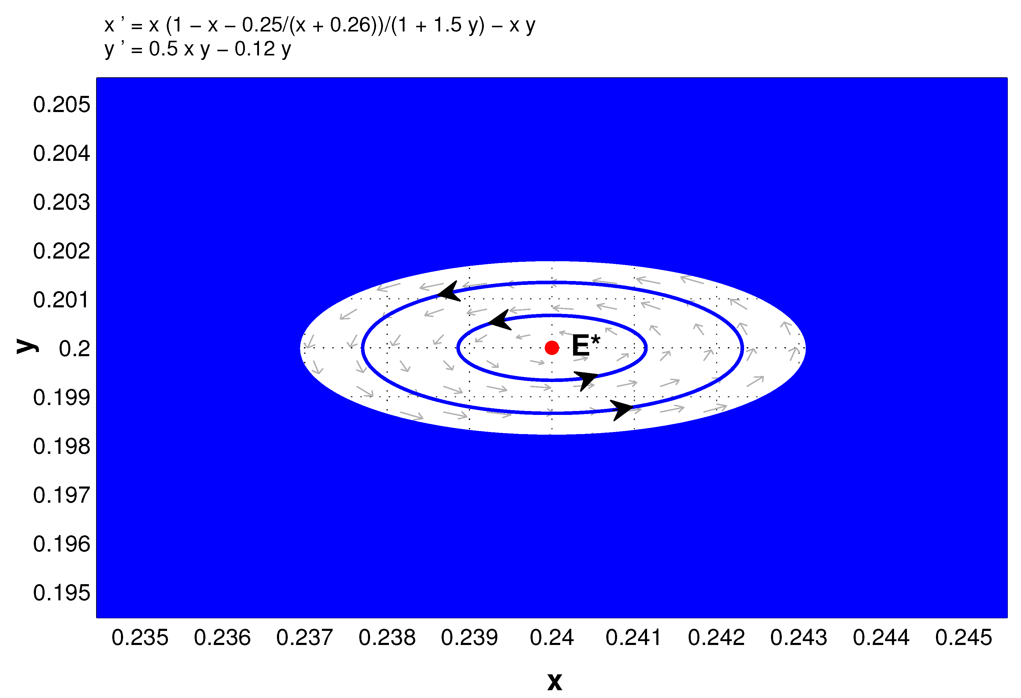
Figure 3 shows the Hopf bifurcation while
Figure 4 further indicates that
is locally stable when
(which can be confirmed with center manifold theory). Here
,
,
,
,
, and
.
6. Numerical Simulations
In
Section 3 and
Section 4, we studied the stability of the equilibria of system (5). In this section, we use numerical simulations to demonstrate different scenarios of the dynamics according to whether
or not.
Example 1. Firstly, we consider the following special case of system (5) with :We distinguish four cases to illustrate the complicated dynamics of system (11). First, we choose
. If
, then the conditions of Theorems 1 and 4–6 are satisfied, and hence, for system (11),
and
are saddle points and
is a stable node (see
Figure 5a); but if
, then
is a saddle point and
is a stable node (see
Figure 5b).
Next, let
. When
, system (11) has a saddle-node
(which coincides with
), a saddle point
, and a stable node
(see
Figure 6a), while when
, it has a saddle-node
(coincides with
) and a stable node
(see
Figure 6b).
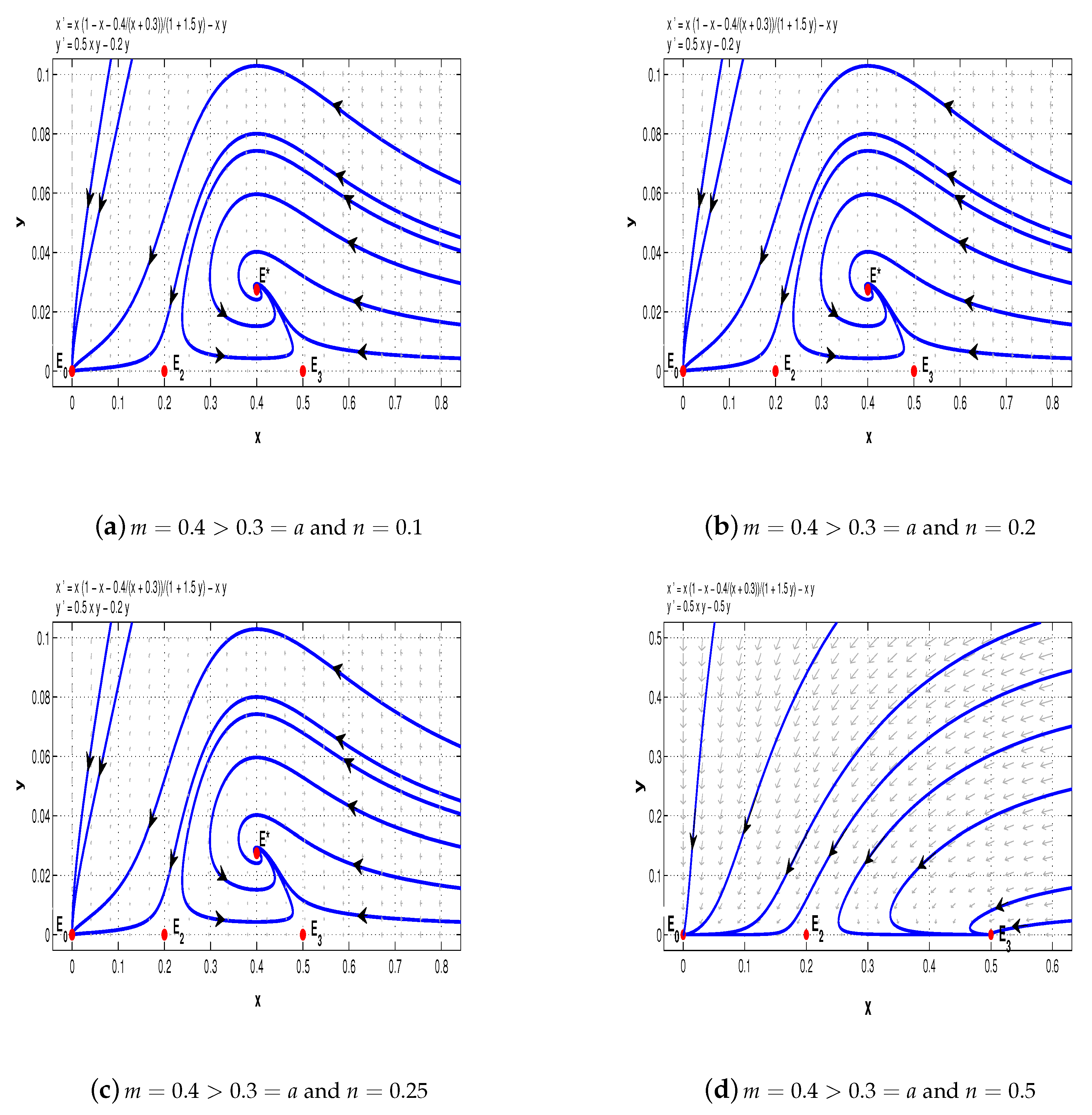
Now, take
. When
, system (11) has a stable node
, a saddle-node
, and a saddle
(see
Figure 7a); when
, there is a stable node
, two saddles
and
, and a stable node
(see
Figure 7b); when
,
is a stable node,
is a saddle, and
is a saddle-node (see
Figure 7c); when
,
is a stable node,
is a saddle, and
is a stable node (see
Figure 7d).
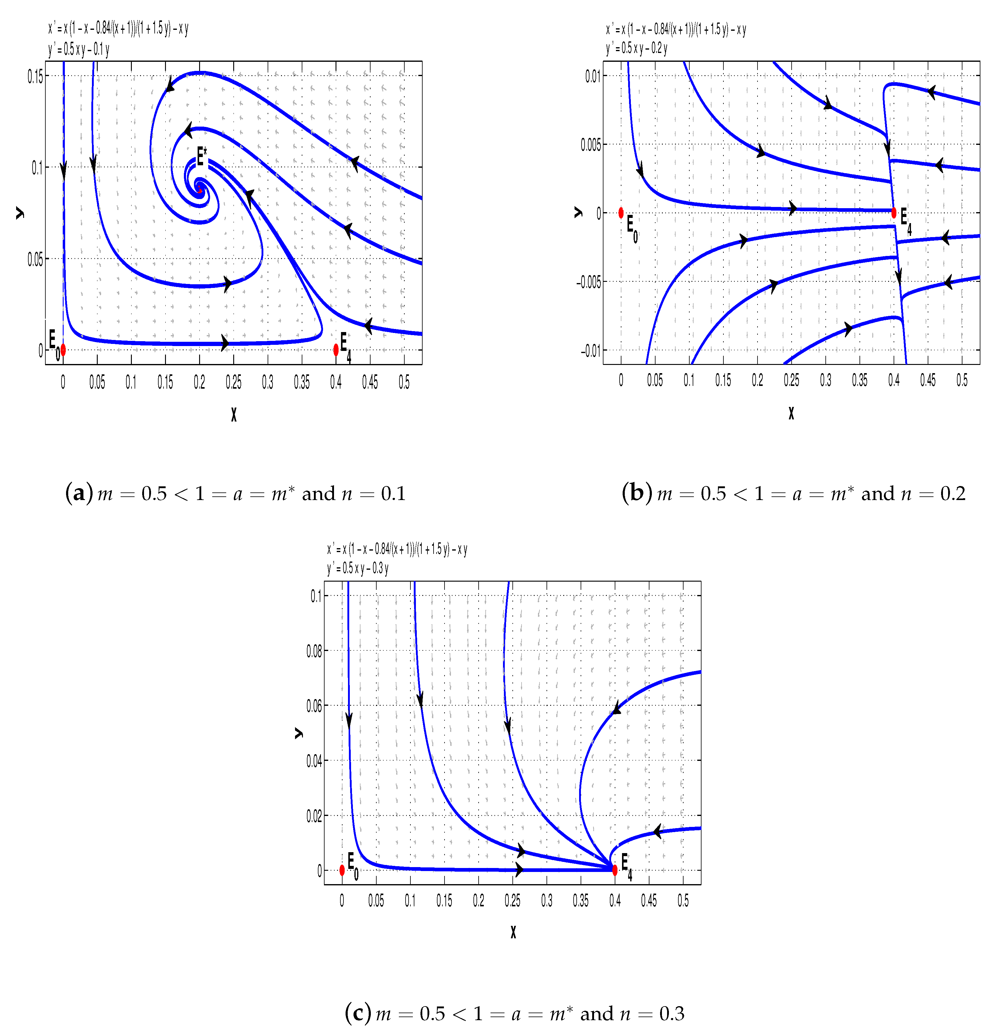
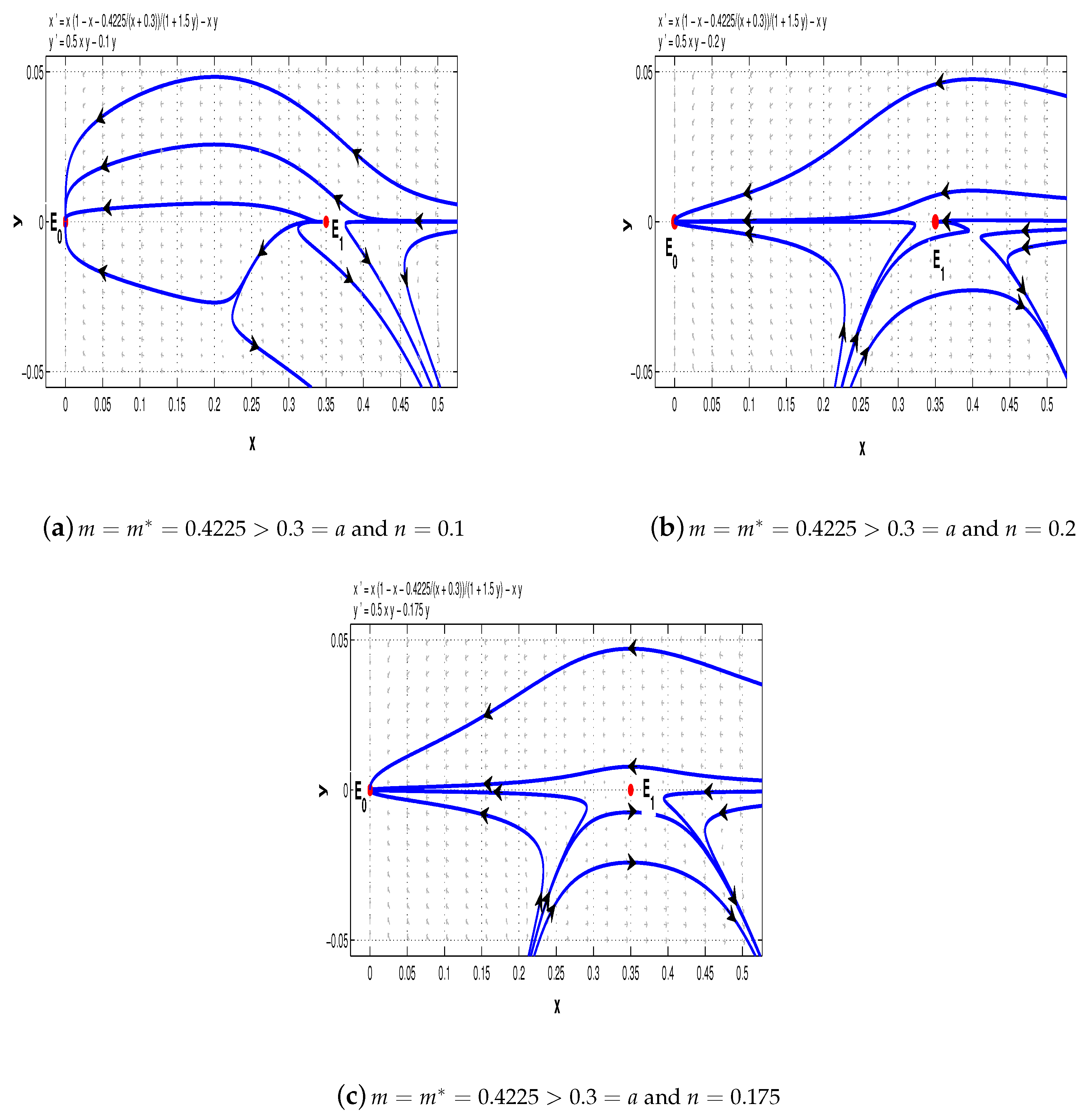
Finally, pick
. When
and
, we see that the equilibrium
of system (11) is a stable node and
is a saddle-node (see
Figure 8a,b); when
,
is also a stable node, however,
is a saddle (see
Figure 8c).
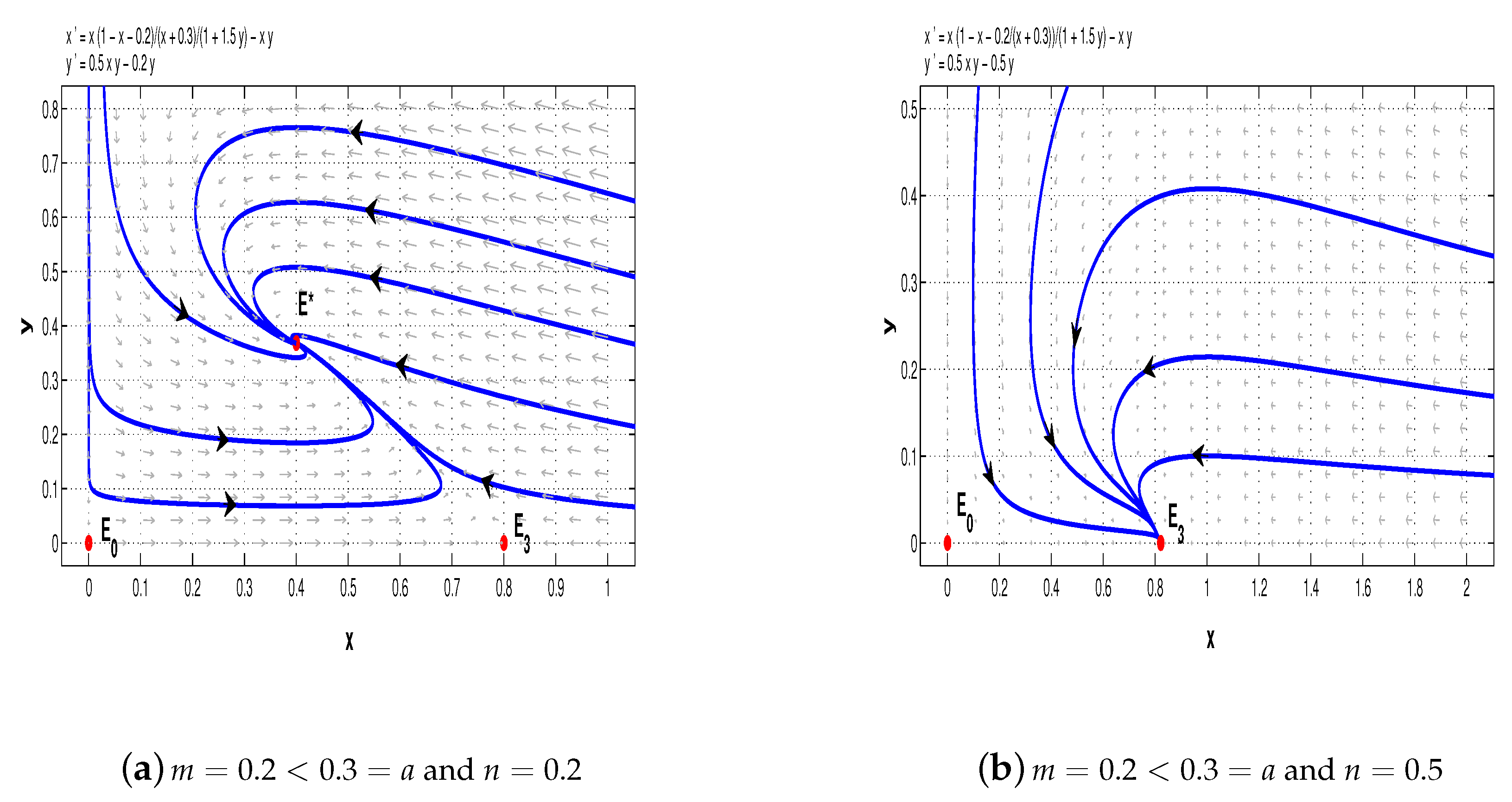
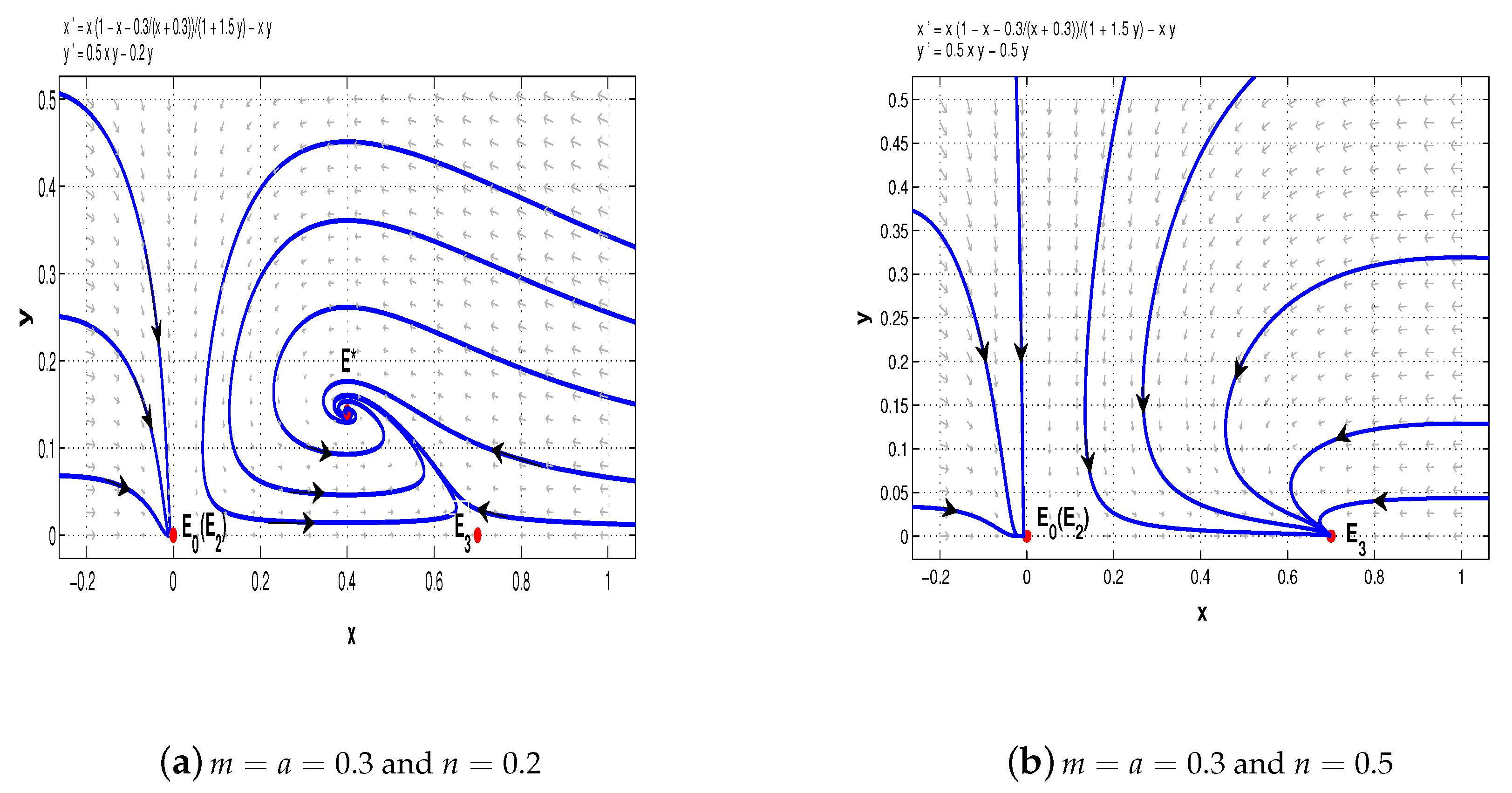
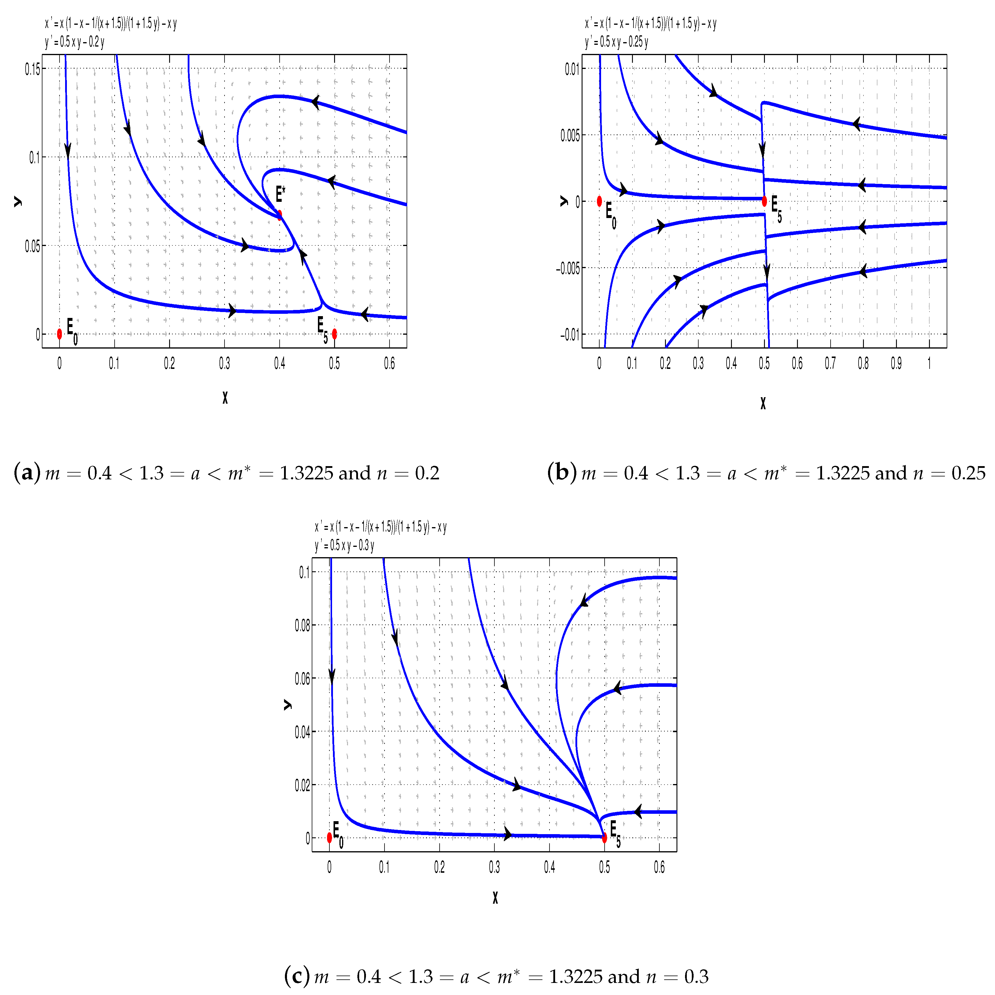
Example 2. This time we let and consider the following system: For system (12), we have
. Choose
. From Theorems 1, 4, and 5, we can see that when
, it has two saddle points
and
, and a stable node
(see
Figure 9a); when
,
is a saddle and
is a saddle-node (see
Figure 9b); when
,
is a saddle and
is a saddle-node (see
Figure 9c).
Example 3. Now we considerwhere . In this case,
. Take
. From Theorems 1, 4, and 5, we can know that we should let
. Then system (13) has two saddle points
and
, and a stable node
(see
Figure 10a); when we let
, it has a saddle point
and saddle-node
(see
Figure 10b); but when we let
, it has a saddle point
and stable node
(see
Figure 10c).
7. Discussion and Conclusions
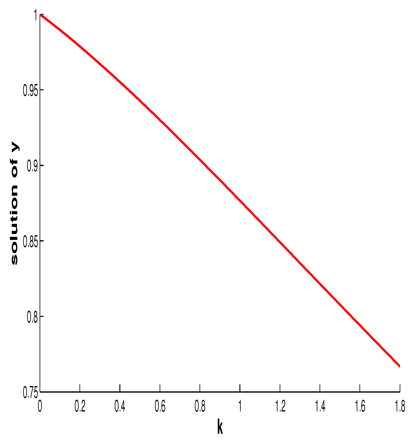
In this paper, we mainly focused on the impact of the additive Allee effect. In this section, we first discuss the influence of the fear effect on the coexistence of the two species. For this purpose, we regard
and
functions of
f. Differentiating both sides of
with respect to
f gives
Thus the fear effect has no influence at the size of the prey at the coexistence equilibrium (final size of prey) but enhancing it will make the final size of the predator decease. This is the same as in [
29,
30].
Figure 11 shows the relationship between the intensity of fear effect and the final size of the predator.
We briefly summarize our findings to conclude this paper below.
In this paper, we proposed and studied a predator–prey model with the additive Allee effect and the fear effect. Though much has been done for predator–prey model with the Allee effect and the fear effect, to the best of our knowledge, the combined impact of these two factors has not been investigated. The findings here have some similarities and differences from those for system (4) with the strong Allee effect. For our model, both additive the Allee effect and the fear effect can affect the number and stability of equilibria. For example, the trivial equilibrium can be a stable node, or a saddle-node, or a saddle point. These results suggest possible bifurcations. By applying Sotomayor’s theorem, we established conditions for the occurrence of saddle-node bifurcation and transcritical bifurcation from boundary equilibria. We also studied Hopf bifurcation from the positive (or coexistence) equilibrium. By calculating the first Lyapunov number, we know that the Hopf bifurcation is supercritical. Finally, the fear effect only affects the final size of the predator. These results indicate that the additive Allee effect can produce much more complex dynamics that the multiplicative Allee effect can.


