Evolution Model for Epidemic Diseases Based on the Kaplan-Meier Curve Determination
by
 ,
,
Jose M. Calabuig
1, 
Luis M. García-Raffi
1 ,
,
Albert García-Valiente
2 and
Enrique A. Sánchez-Pérez
1,* 1
Instituto Universitario de Matemática Pura y Aplicada, Universitat Politècnica de València, Camino de Vera s/n, 46022 València, Spain
2
Universitat de València, Doctor Moliner, 10, 46100 Burjassot (València), Spain
*
Author to whom correspondence should be addressed.
Mathematics 2020, 8(8), 1260; https://doi.org/10.3390/math8081260
Submission received: 27 June 2020
/
Revised: 24 July 2020
/
Accepted: 27 July 2020
/
Published: 1 August 2020
(This article belongs to the Section Mathematics and Computer Science)
Abstract
:We show a simple model of the dynamics of a viral process based, on the determination of the Kaplan-Meier curve P of the virus. Together with the function of the newly infected individuals I, this model allows us to predict the evolution of the resulting epidemic process in terms of the number E of the death patients plus individuals who have overcome the disease. Our model has as a starting point the representation of E as the convolution of I and P. It allows introducing information about latent patients—patients who have already been cured but are still potentially infectious, and re-infected individuals. We also provide three methods for the estimation of P using real data, all of them based on the minimization of the quadratic error: the exact solution using the associated Lagrangian function and Karush-Kuhn-Tucker conditions, a Monte Carlo computational scheme acting on the total set of local minima, and a genetic algorithm for the approximation of the global minima. Although the calculation of the exact solutions of all the linear systems provided by the use of the Lagrangian naturally gives the best optimization result, the huge number of such systems that appear when the time variable increases makes it necessary to use numerical methods. We have chosen the genetic algorithms. Indeed, we show that the results obtained in this way provide good solutions for the model.
MSC:
Primary 62N02; secondary 90C271. Introduction
The epidemic processes caused by viral infections are global problems that affect all human beings. Their understanding, also from a mathematical point of view, is crucial. It provides effective tools for decision makers who are leading the country’s response to the virus to do so in a correct and informed manner. The global crisis of Covid-19 requires a rapid update of mathematical procedures. The aim is to help medical professionals and politicians to understand the dynamic system in a simple way. It must also be deep enough to reflect the current situation, in all aspects of the problem that are truly significant for decision making.
In this paper, we focus on the procedure for determining the Kaplan-Meier (KM) survival curve for the virus that causes the disease. This curve describes the probability that an individual who is infected at the time will continue to be infected after a period of time, when The strategic relevance of this curve is obvious: it is exactly at this time when many countries in the world are beginning to end the period of confinement. A good estimation of this curve could help to know what is the correct period of time after which it is safe to let people go on with their normal lives. In other words, how long it is necessary to wait before the survival of the virus is small enough to be considered insignificant. The risk of new infections after the first wave is also evident as can be seen in many countries at this time. In this way survival curves can help manage the response of health systems.
Table 1 presents the main variables considered in the model. One of the main problems in analyzing the real dynamics is that the way in which different countries are measuring these variables differs greatly. Moreover their values do not correspond at all to the real values of these variables. This was the case, for example, during the Covid-19 pandemic. When mass testing was not possible due to lack of tests caused by strong international demand, sick people were either counted as Covid-19 patients or not, depending on the symptoms. In particular, in some countries (Spain or France) some deaths in nursing homes have not been recorded as deaths caused by Covid-19. In other countries (Germany), deaths of already ill people who eventually died for other reasons but who tested positive for Covid-19 were not recorded as deaths by Covid-19. In addition, a patient was considered free of the virus once they left the hospital. However often returned positive after a few days, or negative several days before leaving the hospital. The decision on how to do this was made with different criteria depending on the region. In fact this was a source of national discussion in countries like Spain, as the interested reader can find in local newspapers from March to May 2019.
This means that, although one might think that the Kaplan-Meier curve of the virus has to be independent of the country—it only depends on the virus itself and how it affects humans, this is not really true: each country has its own viral behavior. From a mathematical point of view, this is not a problem. The prediction that governments are interested in making refers to their own defined variables, as long as this definition is not changed throughout the period. Consequently, each region has its own curve, and similar curves indicate similar variable definitions, rather than the similarity of virus characteristics in different countries.
Choosing the right set of independent variables to fully describe the system could significantly improve the characteristics of the model allowing each country’s data to be modeled in a general scheme based on more variables. This could be done in several ways, depending on the analyst’s point of view. The logrank test can be used to check whether two different populations, for example from different countries, follow the same statistical description. In the context of regression analysis, well-known classical techniques can also be used. This is for instance the case of the comparison of standardized regression coefficients R, or the analysis of the increase in R-squared when a new variable is added to a model that already contains all other variables. The principal values method would also provide a way to look for a reduced set of relevant independent variables. In the case of this paper we will only consider the number of new infected individuals as independent variable, and the number of recovered patients plus the dead as a dependent variable, and so a general study is not considered.
With regard to the Covid-19 crisis, attention has focused on determining the epidemic (epi) curves, which provide an understanding of the global dynamics of the viral pandemic. Updated information on this highly topical subject can be found in References [1,2,3]. The main mathematical models that support the description and forecast of its dynamics are based on the SIR model of the spread of the disease, and on variations of this model. The main objective of this mathematical structure is to predict the values of the main variables after a period of time, which makes it possible to forecast the number of individuals I infected and recovered (plus the dead) E. However, our interest is to calculate a different component of the system, the KM survival curve We will demonstrate that E can be estimated by means of a simple formula that involves the convolution of functions, as
Let us mention that this article is of a mathematical nature, and we are interested in developing a procedure for the calculation of the Kaplan-Meier curve by means of empirical data. Our ideas also allow us to define a transfer model (infected individuals→recovered individuals plus the dead), in which the transfer function is the survival curve, which could help in the management of epidemic processes. We will continuously refer to the Covid-19 pandemic, but it is clear that the mathematical method can be used to control the spread of any similar dynamic process.
The document is structured as follows. In Section 2, a general description of the mathematics used in the paper is given. After a review of the usual methods for dealing with epidemic spread modelling, the variables, basic and general equations of the model—constructed as a convolution of the number of infected individuals and a survival curve that plays the role of a transfer function, are described in Section 2.1, Section 2.2, Section 2.3 and Section 2.4. The least-squares equations to find the best approximation to the real data are shown in Section 2.5, and the exact solution—including the proposed Karush-Kuhn-Tucker conditions—is presented in Section 2.6 and Section 2.7. To complete the overview of methodological approaches, a different model equation based on a (non-linear) fit is briefly explained in Section 2.8.
Section 3 is devoted to showing the results of three different methods to compute approximations to the solution of the equations presented in Section 2. First, a direct Monte Carlo approximation is presented in Section 3.1. The result of the application of a more sophisticated method, based on a sampling on the set of possible linear systems obtained from the Lagrange equation with the Karush-Kuhn-Tucker conditions, is shown in Section 3.2. a genetic algorithm approach is presented in Section 3.3, together with some comments comparing all the proposed methods. Finally, the conclusions are presented in Section 4.
2. Material and Methods
Due to their importance in the control of many health problems, survival curves have been studied from different points of view since their appearance in the mid-20th century [4]. Essentially, they are based on a probabilistic distribution, and their main development has been in statistical terms since their appearance. In the context of infectious diseases, this distribution has some particular characteristics that are currently the subject of formal research. In fact, as explained in References [5,6], current research on the subject focuses on two main statistical methods for infectious disease data. The first consists of the chain binomial models, in which disease transmission is modeled as a discrete time process among individuals. The second is given by the generation interval models, which use continuous time and are based on the idea that disease transmission creates a new category of infected individuals, rather than on the spread through a population of individuals that could be infected.
In any case, these models focus on the individual infections, and the mathematical structures are built around estimates of the associated rates. As we will explain, our methodological approach to the survival curve does not attempt to estimate these rates but considers the curve as the transfer function between the fundamental epidemic variables (number of infected individuals → number of patients recovered plus the dead). Therefore, we do not try to calculate the relevant parameters such as the reproductive number ([5]) but provide a description of the epidemic phenomenon as a transfer process. In addition, research is currently being conducted on determining data from the Kaplan-Meier estimator from other perspectives, such as the computational point of view (see Reference [7] and the references therein).
On the other hand, the most popular mathematical structure that is used in the modelling of infectious diseases during the current Covid-19 crisis is the so called SIR model and modifications of this model, as the so called SEIR, MSIR, SIRD, MSEIR and other compartmental models ([8,9,10,11]). All these models are based on the assumption of the existence of some compartments of individuals who pass through them in successive steps, or die. The SIR model—the most elementary—consists of a system of differential equations that reflects the behavior of the total set of individuals who are susceptible to be infected (S), the number of infected ones (I) and the set of recovered individuals (R) by means of elementary balance equations. The basic model is given by the differential equations
where N is the sum of I and t is the time and and are characteristic constants of the model. Modifications of these equations provide adaptations to different situations, and give the SEIR, MSIR, SIRD, MSEIR and other models (the abbreviations come from the names of the compartments appearing in the model). The origin of these compartmental model can be found in the classical paper, Reference [12] (see also Reference [13]). Note that this formalims allows a global description of the dynamics of the infection. It is assumed that the permanence of an individual in the “compartment of infected people” is a random variable with exponential distribution. The interested reader can find basic definitions, general explanations in the classical book of Bailey [14] and (References [15,16], Ch.I), and current updates in References [10,11] and the references therein.
Let us explain an example of this type of model that can be found in (Reference [10], p. 601). Suppose that a certain infectious disease affects a certain population. If a mother has been infected and cured, some antibodies are transferred to the baby before it is born in such a way that the newborn has a passive immunity to the infection for some period of time. This defines the compartment of passive immunity class M, which passes to the susceptible class S when maternal antibodies disappear, along with children whose mothers were never infected. After contact with an infected individual, they enter the exposed class E of children who are infected but not yet infectious. After the latency period, they enter the class of infective, and, if they survive, become an element of the recovered class This is so an example of a MSEIR model constructed by a passively immune class a susceptible class an exposed class an infective class and a recovered class An empirical approach as the one presented here based on such a compartmental method can be found in Reference [17].
In (Reference [18], Section 2), an exhaustive explanation of which are the limitations of the SIR model is presented. The third of these limitations is that the exponentially distributed duration of infection is assumed; in particular, the model assumes that an individual becomes infectious automatically when is infected, and the probability of recovery does not depend on the time that has passed since infection. As we will explain, none of them is assumed in our model. General criticism to the posibility of foreseeing the dynamics of an epidemic process that should be taken into account are presented in Reference [19]. Some specific software packages have been developed containing the algorithms for solving the related equations; the interesting updated package incidence of R—the software that we use, is explained in Reference [13]. Some specific applications of epidemic modelling using this framework to the current Covid-19 crisis have been already published (see for example Reference [20]).
As we have explained before, our methodological point of view, although related, is significantly different. In the framework of survival analysis, the KM curve represents the estimate of the probability of survival of a standard individual after a time s (see for example References [4,21], ([22], Ch.2), or the general books on mathematical modelling of biological processes cited in the previous paragraphs). This means that no assumption is made on the probabilistic distribution of any variable of the system, and the objective of the calculations is exactly to get some information on this distribution. In this paper we are interested in the determination of this function.
This is the basic element of the model, in which many modifications can be incorporated, for example to introduce continuous variables, or other groups of individuals belonging to the original population with different properties. In any case, the model is always built on the basis of the estimate of the instantaneous probability at a given time In our case, we use a different definition of the notion of deceased, and introduces the possibility of restitution of deceased individuals to the set of non-deceased elements (“resuscitated”, in our case, “reinfected” individuals).
This distribution provides the form of the decreasing function that simulates the decreasing amount of individuals that are considered to be still alive from an initial population. However, to use the data that are given by the statistics provided by governments, for example, the initial population cannot be considered as a fixed set; at each time there is a new group of population entering in the total count of concerned individuals. Thus, other important tool for the description of the dynamics of the system is the function that represents the new contributions to the set given at each time This is the function that usual epidemic models, as the SIR explained above, try to estimate. The simplest one is the classical exponential equation that describes the increasing behaviour of propagation of a virus at the beginning of the epidemic process: for a time the formula
provides the desired estimate in the expansion period of the virus. Here is the initial infection spread rate and K is the infected population when the epidemic process begins. As we will see, the final variable that is desired to be predicted—the number of individuals that are already free of the viral infection—can be forecasted by convoluting this function—either this estimate or directly the real data—with the estimate of the Kaplan-Meier distribution. Recall that the convolution allows to represent the output function E of a transfer process for an input function F when a transfer function G acts on it. It describes how inputs are leaving the system at each time. The deconvolution is the inverse operation: given the function of the inputs to the system F and the function of the outputs it allows the calculation of the transfer function Finally, let us recall that this “deconvoluting” method is needed because the states are publishing global data during the Covid-19 crisis, and not the concrete dates of each patient—starting and final dates of infection. If this information would be available, we could simply put together all the individuals, considering for each one the day she/he started the infection.
For the concrete case on which we focus our attention—the Covid-19 epidemic process—we have to understand the notions of original population and deceased individuals in a different way. We start by defining a fixed set of individuals for whom the infection has been confirmed, and analyze the decrease in this infected population to study the survival of the virus. Therefore, opposite to the way in which the KM distribution is usually interpreted, we consider a fixed group of infected people, and we count as decease when a patient is either considered recovered or dies.
Due to the specific properties of the virus associated to the Covid-19 disease (see for example References [2,3], although the reader can find a lot of information on the internet about this controversial and topical issue), we have to introduce the following new assumptions in order to adapt the model to this case.
- (1)
- There are individuals who test negative for infection but are still able to spread the disease to others. So they should be considered active from the point of view of the virus—as an infected individual—for at least a fixed period of time N.
- (2)
- There are cases that reappear as infected after being counted as recovered individuals.
2.1. Latent Cases and Resuscitation Rate
We start by considering the necessary adaptation of the classical Kaplan-Meier estimate of the instantaneous probability of survival. We are interested in measuring the probability of preservation of the infected population. Thus, we will consider the function to be the probability of survival of the virus at the time that is, the probability that a standard individual who was confirmed as infected in time will continue to be infected in time
We have to introduce a new term representing the “resuscitated cases" at the time which is not considered in the classical formula. It is defined as a function of although the ratio of individuals who are resurrected will be fixed as a constant later in the formalism. Making a simple balance, we obtain the equation
where is the population surviving at the time t—minus the individuals that leave the study, if any, and is the number of individuals leaving the group after the time Note that, in the way we are adapting the model, is the population still having the virus, since we are constructing the survival function of the virus. Therefore, among the individuals who have left the group of infected individuals, we include the recovered patients along with the death patients. Thus, the instantaneous probability is given by
A resuscitation rate can be defined as Using it, we can also define the function
which will be used next and will be assumed to be constant. It should be interpreted as a parameter to measure the rate of resuscitation which has a clear meaning in the model. The estimate of the probability of survival at the time t—the probability that an individual remains infected in our model— is given by
where is the size of the initial confirmed population considered.
2.2. Cumulative Function and Complete Model
Now we describe the dynamics of the system when a continuous increase of the confirmed cases is considered. Following Table 1 we write for the function of time that represents the number of new infected individuals at each time Then total amount of infected patients at a time , , is given by the “convolution formula”
where as mentioned earlier, is the probability that an individual will continue to be infected at the time To what point this equation can be considered as a convolution, and also as the result of the composition of a transfer function with the function describing the new infected individuals, will be explained in Section 2.4.
For example, if the function I is represented at the beginning of the epidemic by an exponential formula as —where K is a positive constant and is the infection spread rate, we get In general, the function I can be obtained by experimentally observing the evolution of the epidemic, or by a functional estimate based on previously observed data.
2.3. Dynamic Estimate of the Number of Post Infection Individuals
Essentially, the model we propose is defined as a transfer process in which there is a daily inflow of new cases , and an outflow of individuals who are no longer infected, and is given as the sum of recovered patients and death patients . These functions depend on the day t, but while the first is defined daily, the second and third are considered cumulative, starting from the first day Thus, we write for newly infected individuals daily, and for the cumulative amount of recovered plus the cumulative amount of the dead Let us now estimate the function which is in a sense the complementary magnitude associated with the function —the total amount of infected patients— explained in the previous section. To simplify, we will assume that the function is in fact a constant rate, so we will write instead of Indeed, the fact that the rate of resuscitation is constant over time (and therefore ), is a reasonable assumption: it means that the proportion of individuals in whom the infection “resuscitates”, is constant at all stages of the epidemic process.
Define the sequence
The quantity represents the probability of an infected individual either to become recovered or to die at the time Thus, we clearly have that
which can be used to construct a system of equations when the time values are considered.
Using the quantities we can compute the value of the characteristic parameters of the model. In particular, for every we have
Note also that, although we are not interested in calculating it here, an estimate of the value of would give an approximate value of Using these expressions, we get
and so
Using also that we obtain the final formula of the model,
This expression allows us to obtain the probability H that the virus survives as the complementary function to the probability that an individual recovers or dies given just above. Thus, the survival function of the virus is defined such as
2.4. Probabilistic Model for the Evolution of a Viral Epidemic Process Based on the Kaplan-Meier Curve
In view of the definitions and formulas given above, we can fix in abstract terms the framework for a simple modelling of the dynamics of a viral process as follows. Recall that, given a couple of integrable functions its convolution is given by
Let us fix the origin of the measure of time at the point The model is represented by the next convolution of functions.
- Let be an integrable function representing the new cases of sick people: represents the number of new patients in the model introduced at the moment
- Let be other integrable function representing the cases that are out of the process at the time t of sick people: is the sum of the dead at that time t plus recovered patients. We can use exponential expressions as the ones explained above
- The function explained above, that represents the probability at the time t of survival of the virus—that is, the probability that a confirmed individual will continue to be infected.
- The formula that gives the relation among these terms is thenAs we have shown in the previous development of our formalism, in this paper we use the discrete version of this formula. That is, is the counting measure. The general model presented by the convolution formula could be used when the entry of new cases can occur at any time, and is not necessarily entered daily. In this case, continuous variables and functions over the Lebesgue measure space seem to be more convenient. But note that the formula describing the model is essentially the same.Note that for some relevant cases we could be interested in (for example, counts of individuals provided by all the countries in the world with Covid-19) we cannot assume that all the individuals that are counted as confirmed (I) are controlled in the process (i.e., some of them were not at any hospital or passed away). In other words, the equation —for M being the dead and F the recovered people—cannot be assumed to hold at the end of the epidemic process in general. So, due to the lack of correct information, we could have infected individuals who have been detected but are not controlled by the health systems. Therefore, we have to consider another (not determined) parameter that represents this fact, such that the balance equation becomes and so is given byHowever, in the rest of the paper we will assume that—having no other source of information—at the end of the process we have that all individuals who were counted as infected have been counted as recovered individuals or the dead.
2.5. Least Squares Fitting of the Model
As usual, we cannot expect the actual data to match the model equations exactly. Therefore, it is necessary to estimate the values of the parameters involved by means of an optimization method applied to the specific error that we explain in what follows. Fix and consider the expression
Since is the function that describes the cumulative probabilities, they define an increasing sequence bounded by so, we can consider the change of variables by means of the positive elements
Now consider the cumulative quantities given by
A simple reordering in provided by the change of variables to shows that we can rewrite in terms of the 2-norm as
We will write for the triangular matrix appearing in this formula. Therefore, the best solution to our model, when s time steps (days) are considered, is given by the solution of the minimization problem under the constraints for given by
It is a classical problem of quadratic programming, and can be solved using classical techniques in numerical analysis. The interested reader can find information about the mathematical techniques on the topic for example in (Reference [23], Ch.16, §16.2). Standard algorithms of optimization of R software could give some general options to solve this problem; however, after checking these computational tools, we have developed our own procedures for doing it, facing the general optimization problem and finding specific exact and approximate solutions for the model. Next, we will explain the exact solution, given by the direct resolution of the optimization problem. However, after checking the method with calculations involving many points (see below), we realized that the direct solution cannot be used with normal calculation capabilities, so we decided to explore other methods. a direct Monte Carlo sampling of the increasing sequence of parameters between 0 and 1 gives rather poor solutions, although some conclusions can be drawn even with this easy procedure. Genetic algorithms have proven to be the best solution for larger data sets. They provide a good compromise on accurate results and computing power, so that a researcher can do the calculations with a personal computer. We will show this in Section 3.
2.6. A Direct Estimate of the Associated Probabilities
Let us fix a numerical value to the bound in the constraint given by the inequality . That is, consider a fixed and change the constraint in the minimization problem given above by where is the parameter of evolution of the rate of non-infected individuals. The optimal value of this parameter has to be determined also in a second step of the process, that will be explained later on in this Section.
Once is fixed, this problem can be solved using different techniques, including numerical optimization and Monte Carlo methods. We will explain in what follows the classical analytic procedure based on the Lagrange multipliers method. This direct approach could be improved by using more sophisticated results on nonlinear programming, based for example on the Karush-Kuhn-Tucker conditions; however, we choose the next algorithm because it gives an easy answer to our optimization.
Step 1. Define the Lagrangian function
and compute the solution of the system
under the constraint
Step 2. In order to do it note that
Now we have to follow the next algorithm. We have to take into account that we have to also consider the case when for some and then we have to remove the corresponding equations given by the row
(a) Suppose first that there are solutions of the system for all the parameters being The system is given—as in the least square method—by the (restricted) normal equations
where is the column vector with each coordinate equal to together with
We check now if for every In this case we stop here, the obtained solution is the better one—it is then given by and
(b) In case there is no such solution to this system, we consider the case when for one removing the -th equation in the system above when is assumed, and solving again the system. We get in this case one equation and one variable less. The rest of the optimal values have to be too. Now we have to solve all the systems of equations that appear following this rule. If there is at least a solution, we have to compute all of them and compare the errors. The one with the smallest error is the right one; in case there are more than one with the smallest error, we take the means.
(c) In case there are no solutions as in b), we take all the couples of variables and and we try to obtain solutions for which the rest of the variables are We take all the couples and take the acceptable solutions (rest of the variables ). Comparing the associated errors, we choose the best one.
(d) If no solution is found in the previous step, we follow in this way (3 variables = 0, 4 variables = 0, ...) until all the equations of the original system dissapear.
Theoretically, we can define in this way a funcion for a certain
Step 3. As we said, the result computed in the previous steps depends on Consequently, for a consistent fitting of the experimental data we need to compute the better parameter In order to do it, we consider the associated error written above, which in fact depends on that is has to be changed by The final solution is then given by solving the optimization problem
Although an analytic procedure could be designed, a Monte Carlo optimization could be enough for getting a reasonable value for
Note that we have to use this algorithm at each step and the values of the estimates of the constants —and so the estimates of the final probabilities of the model —will depend also on the step s that is being computed. Note also that the sequence has to be increasing to preserve the conditions of the model. This implies that, at each step the minimum above has to be computed for the elements that is
what forces to calculate the optimal values for the model sequentially, starting with until the last value of s corresponding to the time of the last experimental data that is available.
Finally, a look to the definition shows that the optimal values of provides a direct picture of the evolution of the system. Indeed, the function
gives the evolution of the rate of recovered individuals plus the dead, what is the desired estimate. Extrapolation of such functions for can be done using for instance a basis of exponential functions. Other factors affecting survival ratios over time can be considered using for instance the Cox regression model for the estimate of the KM curves.
2.7. Incorporating Karush-Kuhn-Tucker Conditions
Other direct method for solving the problem is provided by the calulus of the minimun of under the requirements for and from the point of view of the Karush-Kuhn-Tucker theorem. Let us consider again the change of variables to the ’s as explained in the previous section for reducing the number of constaints, and rewrite in this terms. We follow the notation introduced there.
Fix In this context, our problem is to find the minimum of
under the constraint
The suitable points are those satisfying the Karush-Kuhn-Tucker conditions, that in our case are given by the equations coming from for all k, where
together with some restrictions. Thus, the problem is solved by finding the solution of the system
under the restrictions
We propose the following algorithm. We have to consider two cases, and
Step 1. If we have that and the problem reduces to the case given in Section 2.6, for After getting the solution, we have to check that
Step 2. If we have that the system is given by the equations
Therefore, we have to consider as in the case given in Section 2.6 all the cases defined for all subsets of ’s equal to In each case, if we make the -th equation of the system has to be removed. Remark again that the solution of the linear system so considered would give what of course do not provide not valid answers to the minimization problem.
The final result will be given, for the minimum obtained, by the value of given by
Since we are computing the minimum under global constraints, we do not need in this case to follow Step 3 in the algorithm explained in Section 2.6. Also, the final comments provided in this section about the optimization with respect to are not needed in this case.
2.8. Functional Estimate of the Survival Model
A different approach, but similar in the sense that it is also based on the minimization of the error, is given by assuming a certain functional form for the survival function. Let us consider again the error and suppose that the extension of to a function of real variable can be approximated by minimizing this error by means of a function
Let us show a simple example. An exponential function with negative exponent is a classical model for survival curves. Note that the first N days, the function have to be constant equal to since there are no recovered individuals or the dead; after this point, the easiest case is given by
where b and is a positive parameter that have to be determined. Then we have that
Standard optimization techniques can be used to get the minimum of such function, and the corresponding value of Note that this value depends on the value of and so some extrapolation techniques have to be used to get the best value of Although this option can be taken into account in case there are not good computing tools available, the previous method that we have proposed should give better results. So we center our attention in showing the solution of the problem using these techniques in the next section.
3. Results: Computational Methods for Estimating the Kaplan-Meier Curve
Suppose, as in the rest of the paper, that we have a function representing the new confirmed individuals at a time t and a function that represents the output of viral process (recovered+dead). For the aim of simplicity, and noting before that there is no change in the way the equations are solved, we assume that the delay N is equal to one. Using the basic convolution formula explained in the previous sections, we propose three different methods for the estimate of the minimum that gives the solution to the optimization problem
where s is the last day for which the information is registered, and is the associated cuadratic error
Recall that, following the notation used in the previous sections, is the lower triangular matrix of the cumulative sum of the number of new confirmed cases per day. If s is the last value of t for which we have recorded data, the final Kaplan-Meier function that represents the decreasing probability of the virus to survive is given by
where is the parameter of progression of the epidemic disease; it will be also optimized in our model. With the aim of simplicity, and taking into account that an amount of confirmed people were considered already free of the virus the same day that they were recorded as confirmed at the hospitals, we will consider the case for checking the method. Further optimizations can be designed to get also the optimal value of N in the model. We use R software for the algorithms and computations.
In order to compare the solutions provided by the different methods, we use the data record of the first 24 days of the Covid-19 epidemics in Spain. The values are shown in Table 2.
Recall that, according to Table 1, the function is the daily entry of new confirmed individuals and stands for the corresponding dead in the public health system. They are shown in Figure 1.
The first 18 days the number of recovered patients was not registered. All the corresponding healed patients were registered together the 19th day; this day 498 new cases appear. In order to get some reasonable data for the example, we have exponentially distributed these cases through the dates from 1 to 21. The distribution formula was fitted using the data from day 25 to day 35. The final equation used to simulate these points is
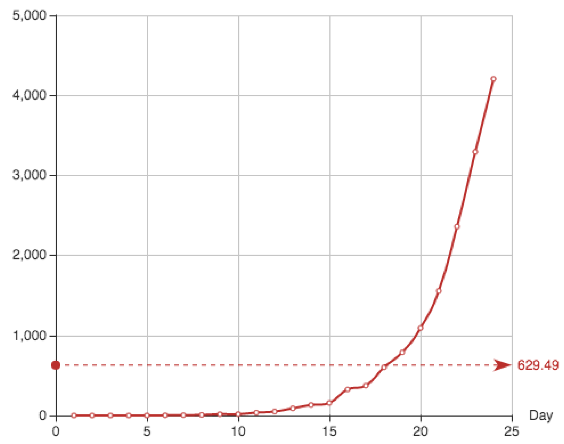
The function is given by cumulative sum of the addition of the recovered individuals and the dead. It is shown in Table 4 and Figure 3.
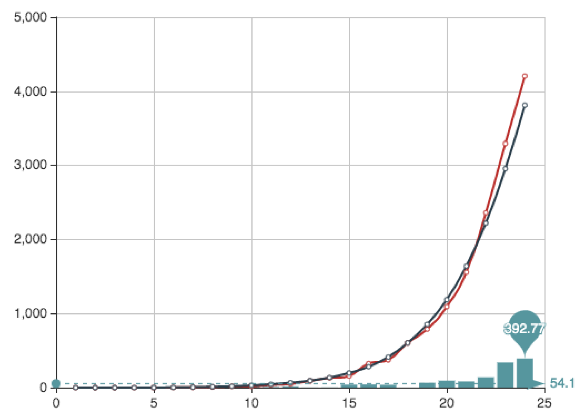
The first proposed procedure to find a good approximation to the solution is a crude Monte Carlo method, in which a big amount of 23-coordinates vectors of possible solutions of the parameters are considered. The second one uses also a probabilistic sampling, this time over the set of all points satisfying the Karush-Kuhn-Tucker conditions that provide suitable local minima. The last one uses also a direct strategy of optimization based on genetic algorithms.
3.1. Monte Carlo Direct Approach
We compute the error for a big set of vectors in the positive part of the unit ball of the -dimensional space and choose the one with the minimum error. For doing it, we take such kind of vectors uniformly distributed on the unit sphere of this space. Then we get randomly its norm uniformly in In order to obtain a (quasi-)uniform distribution on all the set, we weight more vectors that are close to be norm one by weighting the norm obtained in the uniform distribution by writing a power of this function as for a certain exponent that can be adapted to improve the result. The script used is:
- ### Define the error function using matrix J and vector E
- ErrorVec<-function(v){norm((J)%*%v-E, type="2")}
- ### Fix the expo parameter
- expo<-10
- ### Starting variables
- mc<-c(1:24)
- mcfin<-c(1:24)
- ermc<-100000000
- for(k in 1:1000000){
- mc0<-runif(24, min=0, max=1)
- mc<-(mc0/sum(mc0))*(runif(1, min=0, max=1))^(1/expo)
- if(ErrorVec(mc) > ermc ){mc<-c(1:24)*0}
- ermc<-min(c(ermc, ErrorVec(mc)))
- if(ErrorVec(mc)<=ermc){mcfin<-mc}
- }
The main advantage of the method is that it provides a direct estimate of the behavior of the set of solutions. For instance, it allows to understand if the variations of the associated errors is big when a random election is made. In what follows we show the errors associated to the crude Monte Carlo approximation (MC) with and the associated errors in Table 5, showing that the best solution is found for
The associated coefficients for this case— mcfin in the script—written in the natural order are presented in Table 6 (we write only 4 digits).
3.2. Sampling on the Configurations of Local Minima of the Optimization Problem Using Karush-Kuhn-Tucker Conditions
Under the restrictions established in the Lagrangian by the constrains of the problem, a configuration (a vector) where no coincide, represents the variables that are assumed to be 0 and, at the same time, the equations that are removed from the system of linear equations (see Step 2 in the algorithm of Section 2.6). The algorithm can be divided into two cases:
(1) The restriction is assumed. In this case we use three auxiliary matrices (QQ0, QQ1 and ult0) that allow to write and solve the linear systems with the necessary requirements explained in the resolution method. This is done by using the script:
- QQ0<- matrix(nrow = s, ncol = s, byrow = FALSE, dimnames = NULL)
- for(j in 1:s){
- for(k in 1:s){
- if(k>j+1 | k<j ) {
- QQ0[j,k]<-0
- } else {if(j==k & j<s){QQ0[j,k]<-1} else{QQ0[j,k]<--1}}
- QQ0[s,s]<-0
- }
- }
- QQ1<- matrix(nrow = s, ncol = s, byrow = FALSE, dimnames = NULL)
- for(j in 1:(s-1)){
- for(k in 1:s){
- QQ1[j,k]<-0
- QQ1[s,k]<-1
- }
- }
- ult0<-rep(0,s)
- ult0[s]<-1
For the solution of the systems (with the corresponding error) we use the functions:
- ### Exact solution without removing any equation:
- Z<-solve(QQ0%*%t(J)%*%J+QQ1,QQ0%*%t(J)%*%E+ult0)
- ### Adapted functions providing the solution and the error
- ### when the equations labeled by the vector w are removed.
- Sol1<-function(w){
- m<-c(1:length(w))
- A<-QQ0[-m,-m]%*%((t(J)%*%J)[-w,-w])+QQ1[-m,-m]
- b<-QQ0[-m,-m]%*%(t(J)%*%E)[-w]+ult0[-m]
- Sol1<-solve(A,b)}
- Error1<-function(w){norm((J[,-w])%*%Sol1(w)-E, type="2")}
Once again, a sampling technique that goes through all possible configurations of this type provides an estimate of the minimum. Of course, if the computing power is sufficient to calculate the solutions to all these configurations and the associated errors, an exact solution will be obtained. Since a direct sampling could repeat the configurations (the same numbers in a different order), we can restrict the search to sequences of increasing numbers. The corresponding script for this Monte Carlo’s approximation of the solution is:
- er<-100000
- Sol2<-c(1:s)
- for(q in 1:(s-2)){
- for(k in 1:10000){
- w<-c(sample(1:s, q,replace=F))
- cc<-0
- for(u in 1:(s-q)){
- if(Sol1(w)[u] >= -0.00001)
- cc<-cc+1
- }
- if( cc==(s-q) & er >= Error1(w))
- { er <- Error1(w)
- Sol2<-Sol1(w)
- w1<-w
- }
- }
- }
- ### ErrorCaseEqual1 is the error for this case
- ErrorCaseEqual1<-er
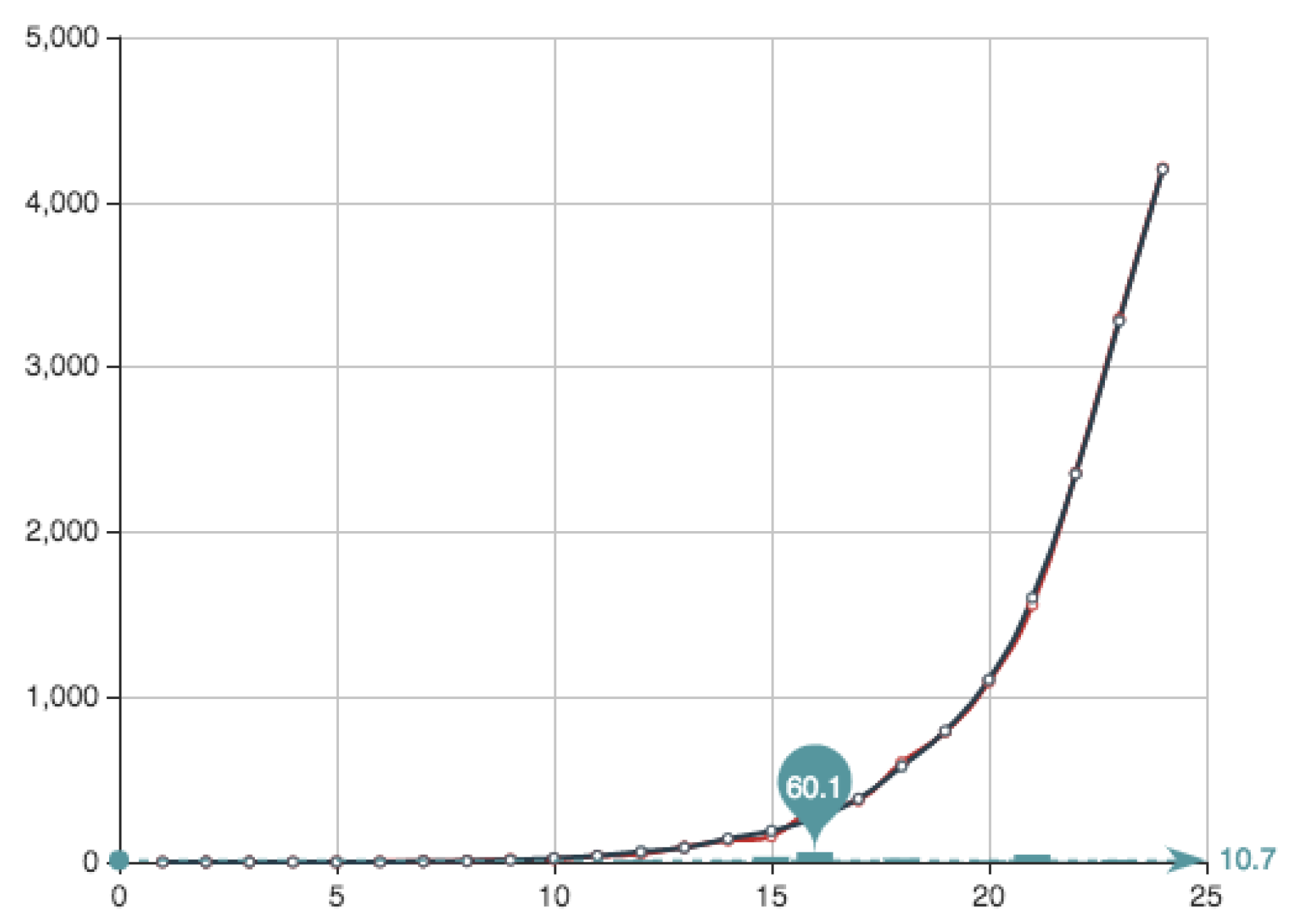
After checking iterations given by sets of n non zero coefficients, for we obtain an error Figure 5 shows the estimate provided for the function E associated to this solution, together with the function E itself. It can be seen that the approximation and the real data almost coincide. Superposition of graphs shows almost 100% of coincidence.
(2) The condition is assumed. The script used for this is:
- er<-100000
- for(q in 1:(s-2)){
- for(k in 1:10000){
- w<-c(sample(1:s, q,replace=F))
- if(sum(Sol(w))<=1){
- cc<-0
- for(u in 1:(s-q)){
- if(Sol(w)[u] >= -0.00001)
- cc<-cc+1
- }
- if( cc==(s-q) & er >= Error(w))
- { er <- Error(w)
- ### Sol0 is the solution
- Sol0<-Sol(w)
- ### w0 indicates which are the equations that have to be removed
- w0<-w
- }
- }
- }
- }
- ### ErrorCaseLess1 is the error for this case
- ErrorCaseLess1<-er
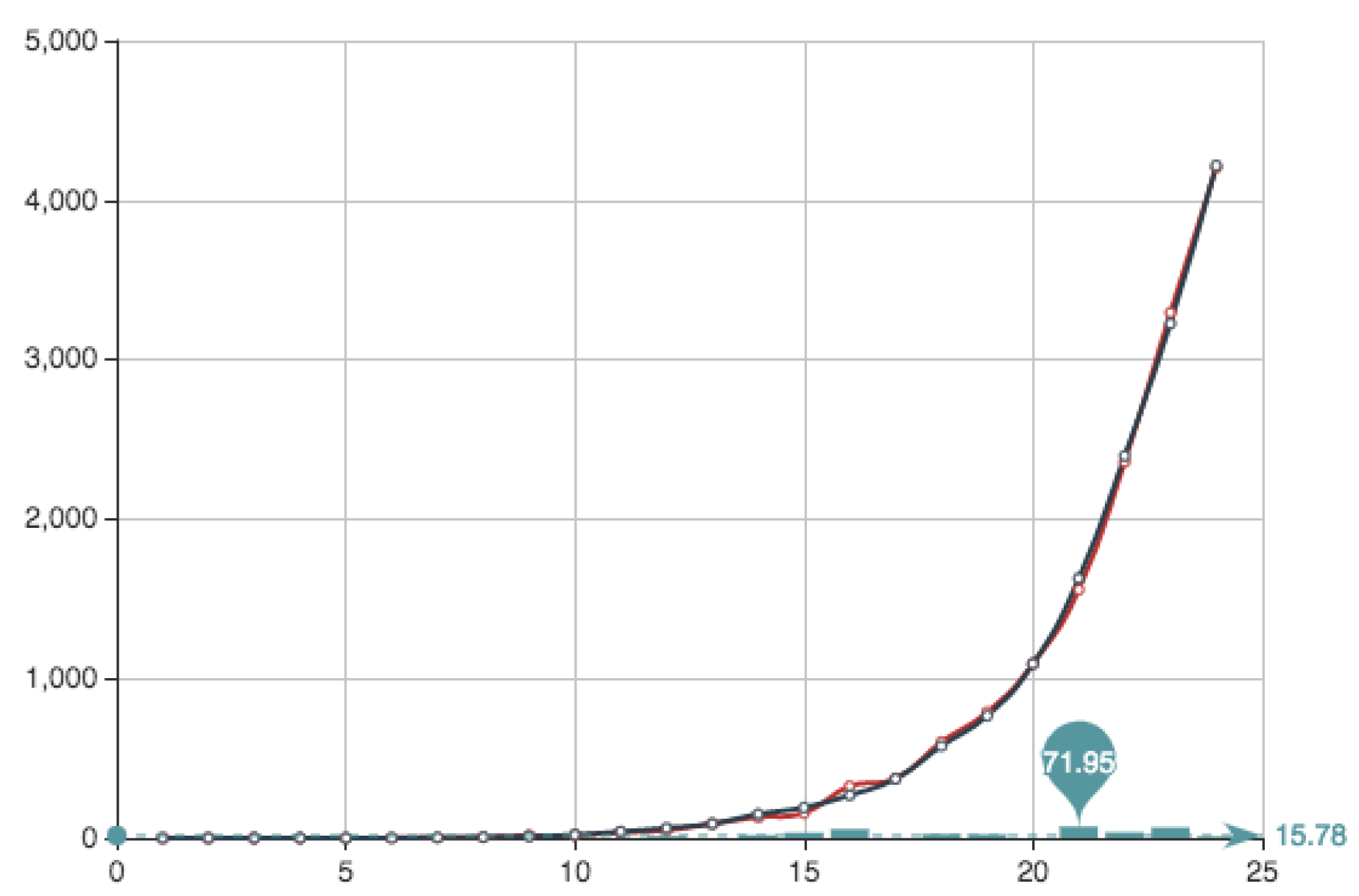
Now, after checking iterations defined by sets of n non zero coefficients, for we obtain an error Figure 6 shows the estimate provided for the function E associated to this solution, together with the function E itself. It can be seen that the approximation and the real data almost coincide. Superposition of graphs shows almost 100 % of coincidence.
Figure 7 shows the survival functions associated to the three approximations that we have presented using different sampling techniques. They can be compared with the one obtained using genetic algorithms in next subsection.
3.3. Genetic Algorithms
A Genetic Algorithm (GA) has been used to calculate an approximated solution of the problem. GAs belong to the category of evolutionary algorithms (EAs), which mimic biological evolution and are based on populations of individuals, where every individual is, in general, a vector from the search space that is a candidate to be a solution the problem. These candidates should be evaluated using a fitness function [24]. We get profit on both the good results obtained with GAs, together with their capability to handle a wide variety of problems with different degrees of complexity, what explains their wide use. Our GA have been designed for getting an approximate solution to the problem by defining a new error that balances the error and the estimate of the cumulative sum where can be handled to improve the result using additional information, starting for example with We define as a fitness function:
where and are weights to balance the terms in the error, being chosen on the basis of the observed convergence properties. The second term of this error function is in fact a constrain over the first part. In the minimization problem it is given by the inequality . The quotient plays the role of “adjustment variable”, being and .
We have used the GA Package in r [25,26] and we have defined a real-valued GA problem with variables . As the genetic algorithm maximizes, we have used as a fitness function . The algorithm has two arguments that influence in its convergence: the population size (popSize) that represents the number of possible solutions that the algorithm evaluate—with the fitness function—in each iteration and the total number of iterations (maxiter). The GA algorithm progress applying the genetic operators (crossover and mutation) to the members of the population to produce the offsprings that will form part of the population in the next iteration ( [24]). We have considered values of the popSize of 100, 250 and 500 in combination with maxiter that takes values equal to 5000, 250,00 and 50,000. In Table 8 we can see values of the relative error, defined as the norm of the difference between the approximated solution obtained with GA and the solution obtained in Section 3.2. The bigger the number of iterations and the population size, the lower the error.
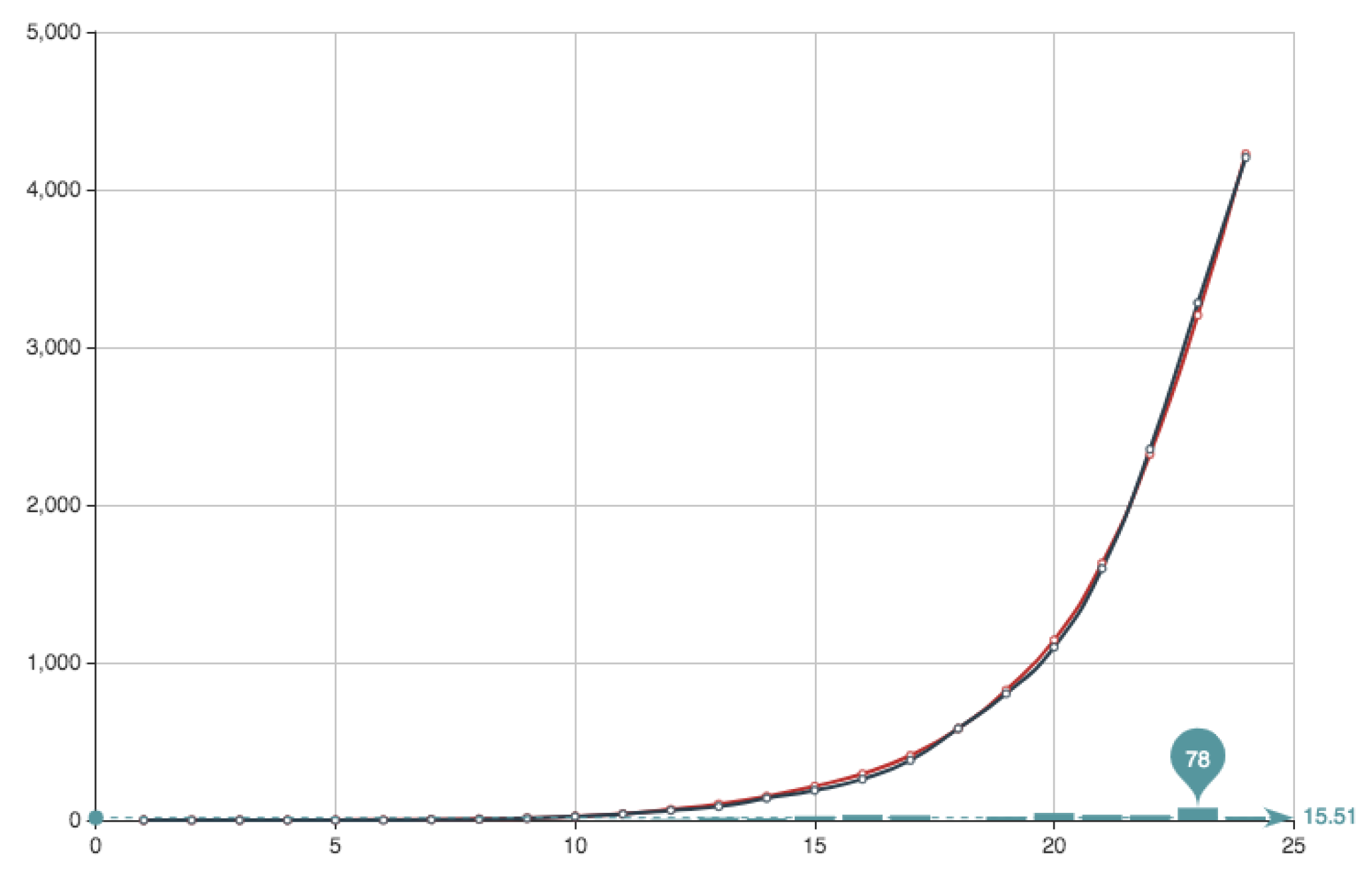
Taking into account the increase in the CPU time when we increase both, number of iterations and population size and the lowering in the relative error obtained, we have fix the values maxiter = 50,000 and popSize. CPU time in a Macbook 2015 (Dual-Core Intel Core i5 2,7 GHz) with 8GB of memory laptop takes less than 30 min. For these values fixed, we have study for this particular case the value of the quotient for which we obtain the best approximated solution. This has been obtained for a value . The solution obtained can be seen in Figure 8 and Figure 9. It can be observed that the approximation is very good, being the error very small. This value of the quotient means that, in this particular case, the first part of the error function is much more important that the second part relative to the condition . Anyway we want to point out that the extreme values and —that is possible to implement numerically—do not produce an acceptable solution or, in other words, the condition is necessary for obtaining a good approximation. Finally, this is not the general situation and, with real data from Covid-19 ([27]) the best fitting is obtained with much more balanced quotient, being the usual value .
The algorithm to implement GA calculation is the next:
- library("GA")
- ### Built matrix J with Data.
- s<-23 ### Dimension of the problem
- ### Define the error function using matrix J and vector E
- ErrorVec<-function(v){norm((J)%*%v-E, type="2")}/norm(E)
- ### Vector v is the solution of the problem
- ### Define the fitness function
- fitness <- function(x) 1/(g1*ErrorVec(v)+g2*abs(sum(v)-mu_s))
- ### Starting variables
- mu_s<-1
- g1<-1
- g2<-1
- ### Define upper and lower bounds for the values
- ### of the components of vector v
- lb <- rep(0,s)
- ub <- rep(1,s)
- ### Finally with fixed labels monitor=’FALSE" to
- ### avoid the printscreen.
- ### See documentation for more details.
- Ga <- ga(type = "real-valued", fitness = fitness,
- lower=lb, upper = ub,
- popSize=250, maxiter=50000, monitor=’FALSE’,
- seed=123456)
- ### Solution is save in variable Sol
- Sol<-c(GA@solution)
In short, as the reader can see, the Monte Carlo method applied directly provides a weak approach to the solution of the problem. The best solution is clearly obtained when sampling over the set of all the systems of equations that describe the local minima. This combination of exact solutions of linear systems with Monte Carlo sampling gives good solutions—even the ’exact’ solution for small datasets, but poses the problem of needing powerful computational tools when the size of the datasets increases. This is due to a “combinatorial” growth of the number of systems of equations coming from the Lagrange equation together with the associated Karush-Kuhn-Tucker conditions. Finally, compared with the results in Figure 7, genetic algorithms provide very good results, as can be seen in Figure 8 and Figure 9, even when the dataset is large. The reader can find some calculations with larger datasets than those in this example in Reference [27] using this method.
4. Conclusions
We have shown a general model to calculate and describe the Kaplan-Meier curve of the virus in an epidemic process, in which the information is given as aggregated data per day: confirmed individuals, recovered individuals and the dead. The use of the survival curves obtained in this way could help in the management of resources for the response to an epidemic process at all levels: at the national level—to know the response capacity of a national health system in an emergency situation, at the local level—in a city, for the management of patients between different health centers, or at the hospital level—for example, to forecast the number of beds that might be needed.
We have made a complete mathematical study of the model, finding the main equations that describe it and proposing different methods to solve them, in order to represent the final results as modeling curves and survival curves. Thus, an analysis of how to solve the equations is given, from a crude Monte Carlo method, the description of the exact method of solution mixed with Monte Carlo search in the space of the local minima, and the use of a genetic algorithm.
Supplementary Materials
The following are available online at https://www.mdpi.com/2227-7390/8/8/1260/s1. HTML versions of the figures can be found as supplementary material. The data are taken from the public repositories on Covid-19 (published by the Spanish Government), and are not interesting in themselves as far as this article is concerned.
Author Contributions
All the authors have contributed equally to the present work, in the creation of the general model and its mathematical construction. In addition, J.M.C. has been in charge of the algorithm and the graphics, L.M.G.-R. has been in charge of the calculations, A.G.-V. has attended to the biological meaning and the fit of the model with the epidemic process it represents, and E.A.S.-P. has designed the general mathematical framework and its formalization. Conceptualization, A.G.-V.; Formal analysis, E.A.S.-P.; Investigation, J.M.C., L.M.G.-R., A.G.-V. and E.A.S.-P.; Methodology, L.M.G.-R.; Validation, L.M.G.-R. and A.G.-V.; Visualization, J.M.C. All authors have read and agreed to the published version of the manuscript.
Funding
This research was funded by Ministerio de Ciencia, Innovación y Universidades: MTM2016-77054-C2-1-P and Generalitat Valenciana: Cátedra de Transparencia y Gestión de Datos (U.P.V.).
Acknowledgments
The authors would like to thank the referees for their valuable comments which helped to improve the manuscript. The author gratefully acknowledge the support of Cátedra de Transparencia y Gestión de Datos, Universitat Politècnica de València y Generalitat Valenciana, Spain. The last author gratefully acknowledges the support of the Ministerio de Ciencia, Innovación y Universidades (Spain) and FEDER under grant MTM2016-77054-C2-1-P.
Conflicts of Interest
The authors declare no conflict of interest.
References
- Ai, T.; Yang, Z.; Hou, H. Correlation of Chest CT and RT-PCR Testing in Coronavirus Disease 2019 (COVID-19) in China: A Report of 1014 Cases. Radiology 2020, 200642. [Google Scholar] [CrossRef] [Green Version]
- Chen, D.; Xu, W.; Lei, Z.; Huang, Z.; Liu, J.; Gao, Z.; Peng, L. Recurrence of positive SARS-CoV-2 RNA in COVID-19: A case report. Int. J. Infect. Dis. 2020, 93, 297–299. [Google Scholar] [CrossRef] [PubMed]
- Monto, A.S.; Cowling, B.J.; Peiris, J.S.M. Coronaviruses. Viral Infect. Hum. Epidemiol. Control 2014, 199–223. [Google Scholar] [CrossRef]
- Kaplan, E.L.; Meier, P. Nonparametric estimation from incomplete observations. J. Am. Stat. Assoc. 1958, 53, 457–481. [Google Scholar] [CrossRef]
- Kenah, E. Contact intervals, survival analysis of epidemic data, and estimation of R0. Biostatistics 2011, 12, 548–566. [Google Scholar] [CrossRef] [PubMed] [Green Version]
- Kenah, E. Non-parametric survival analysis of infectious disease data. J. R. Soc. Ser. B (Stat. Methodol.) 2013, 75, 277–303. [Google Scholar] [CrossRef] [PubMed] [Green Version]
- Ogluszka, M.; Orzechowska, M.; Jedroszka, D.; Witas, P.; Bednarek, A.K. Evaluate Cutpoints: Adaptable continuous data distribution system for determining survival in kaplan-meier estimator. Comput. Methods Programs Biomed. 2019, 177, 133–139. [Google Scholar] [CrossRef] [PubMed]
- Brauer, F. Compartmental models in epidemiology. In Mathematical Epidemiology; Springer: Berlin/Heidelberg, Germany, 2008; pp. 19–79. [Google Scholar]
- Choisy, M.; Guegan, J.F.; Rohani, P. Mathematical modeling of infectious diseases dynamics. In Encyclopedia of Infectious Diseases: Modern Methodologies; Tibayrenc, M., Ed.; John Wiley & Sons: Hoboken, NJ, USA, 2007; Chapter 22; pp. 379–404. [Google Scholar] [CrossRef] [Green Version]
- Hethcote, H.W. The mathematics of infectious diseases. SIAM Rev. 2000, 42, 599–653. [Google Scholar] [CrossRef] [Green Version]
- Silal, S.P.; Little, F.; Barnes, K.I.; White, L.J. Sensitivity to model structure: A comparison of compartmental models in epidemiology. Health Syst. 2016, 5, 178–191. [Google Scholar] [CrossRef] [Green Version]
- Kermack, W.O.; McKendrick, A.G. A Contribution to the Mathematical Theory of Epidemics. Proc. R. Soc. A 1927, 115, 700–721. [Google Scholar]
- Kamvar, Z.N.; Cai, J.; Pulliam, J.R.; Schumacher, J.; Jombart, T. Epidemic curves made easy using the R package incidence. F1000 Res. 2019, 8, 139. [Google Scholar] [CrossRef] [PubMed] [Green Version]
- Bailey, N.T. The Elements of Stochastic Processes with Applications to the Natural Sciences; John Wiley & Sons: New York, NY, USA, 1990; Volume 25. [Google Scholar]
- Bastin, G. Lectures on Mathematical Modelling of Biological Systems. Available online: http://citeseerx.ist.psu.edu/viewdoc/download?doi=10.1.1.465.8665&rep=rep1&type=pdf (accessed on 27 March 2020).
- Keeling, M.J.; Danon, L. Mathematical modelling of infectious diseases. Br. Med. Bull. 2009, 92, 33–42. [Google Scholar] [CrossRef] [PubMed]
- Brown, G.D.; Oleson, J.J.; Porter, A.T. An empirically adjusted approach to reproductive number estimation for stochastic compartmental models: A case study of two Ebola outbreaks. Biometrics 2016, 72, 335–343. [Google Scholar] [CrossRef] [PubMed]
- Huppert, A.; Katriel, G. Mathematical modelling and prediction in infectious disease epidemiology. Clin. Microbiol. Infect. 2013, 19, 999–1005. [Google Scholar] [CrossRef] [PubMed] [Green Version]
- Paul, M. Foreseeing the future in infectious diseases: Can we? Clin. Microbiol. Infect. 2013, 19, 99–992. [Google Scholar] [CrossRef] [PubMed] [Green Version]
- Roosa, K.; Lee, Y.; Luo, R.; Kirpich, A.; Rothenberg, R.; Hyman, J.M.; Yan, P.; Chowell, G. Short-term forecasts of the COVID-19 epidemic in Guangdong and Zhejiang, China: February 13–23, 2020. J. Clin. Med. 2020, 9, 596. [Google Scholar] [CrossRef] [PubMed] [Green Version]
- Jiang, H.; Fine, J.P. Survival analysis. In Topics in Biostatistics; Humana Press: Totowa, NJ, USA, 2007; pp. 303–318. [Google Scholar]
- Kleinbaum, D.G.; Klein, M. Survival Analysis; Springer: New York, NY, USA, 2010. [Google Scholar]
- Nocedal, J.; Wright, S. Numerical Optimization; Springer Science & Business Media: Berlin, Germany, 2006. [Google Scholar]
- Yu, X.; Gen, M. Introduction to Evolutionary Algorithms; Springer-Verlag: Berlin, Germany, 2010. [Google Scholar]
- Scrucca, L. Package ‘GA’-CRAN-R Project. Available online: https://luca-scr.github.io/GA/ (accessed on 27 March 2020).
- Scrucca, L. GA: A Package for Genetic Algorithms in R. J. Stat. Softw. 2013, 53. [Google Scholar] [CrossRef] [Green Version]
- Calabuig, J.M.; García-Raffi, L.M.; García-Valiente, A.; Sánchez-Pérez, E.A. Kaplan-Meier type survival curves for COVID-19: A health data based decision-making tool. arXiv 2020, arXiv:2005.06032. [Google Scholar]
Figure 1.
Daily data of new confirmed individuals (black line) and the new dead (red line). The dashed lines indicate the corresponding average. (Figures in HTML format are in Supplementary Materials).
Figure 1.
Daily data of new confirmed individuals (black line) and the new dead (red line). The dashed lines indicate the corresponding average. (Figures in HTML format are in Supplementary Materials).
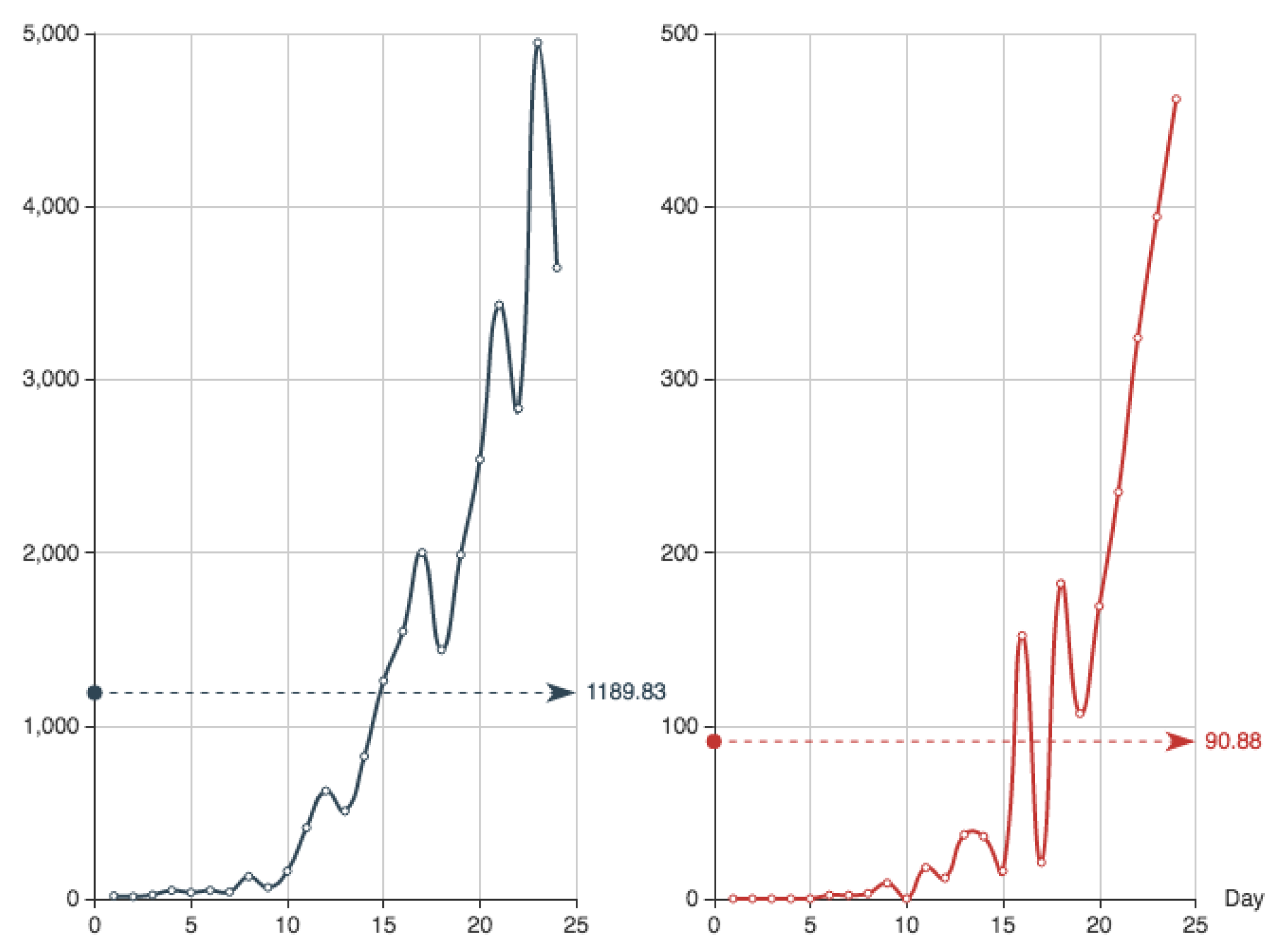
Figure 2.
Simulation of the daily hospital discharges given by the function F. The dashed line is the average and the mark point is the maximum.
Figure 2.
Simulation of the daily hospital discharges given by the function F. The dashed line is the average and the mark point is the maximum.
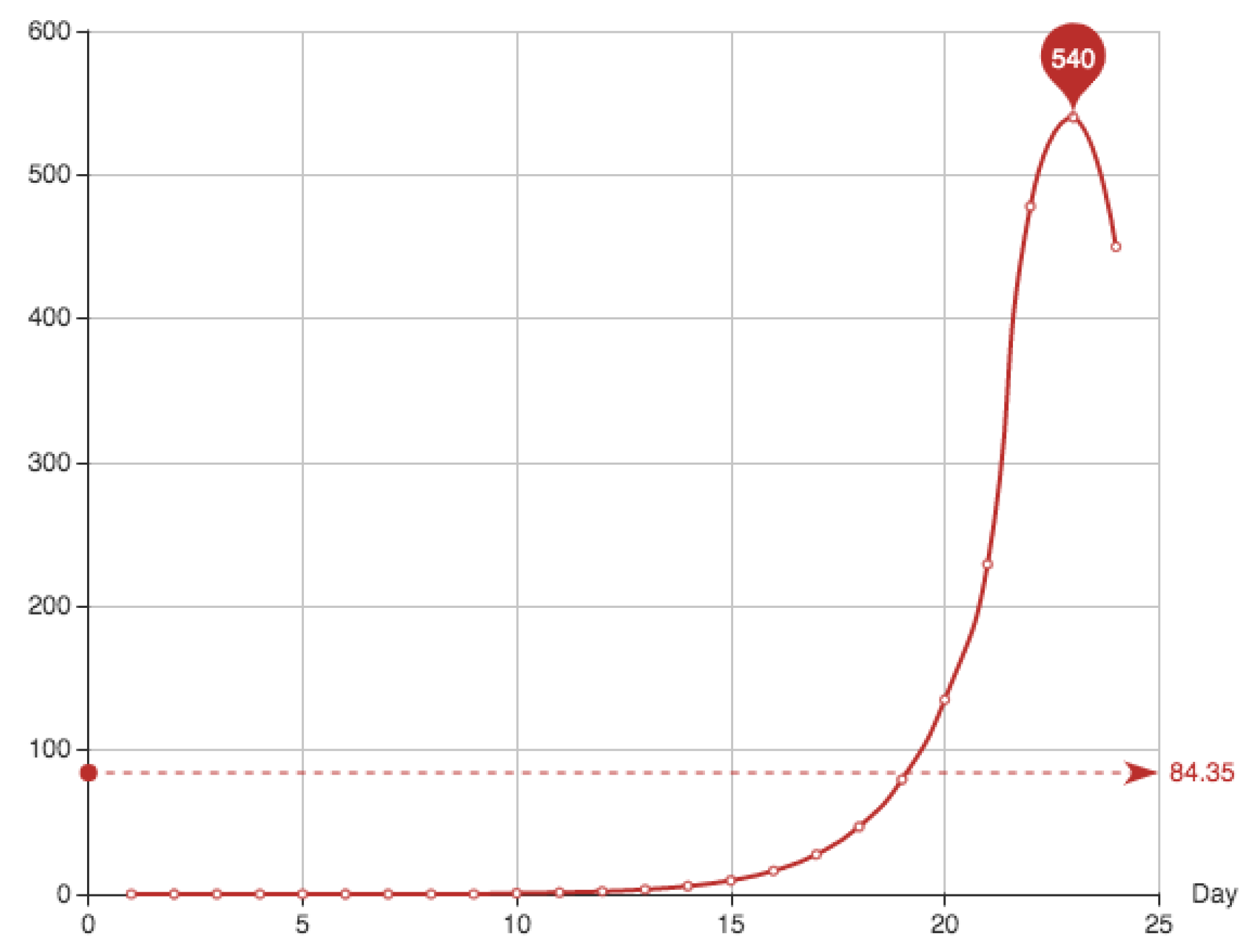
Figure 3.
Actual data of the cumulative sum function E, that is, the cumulative sum of the dead plus recovered individuals. The dashed line corresponds to the average.
Figure 3.
Actual data of the cumulative sum function E, that is, the cumulative sum of the dead plus recovered individuals. The dashed line corresponds to the average.

Figure 4.
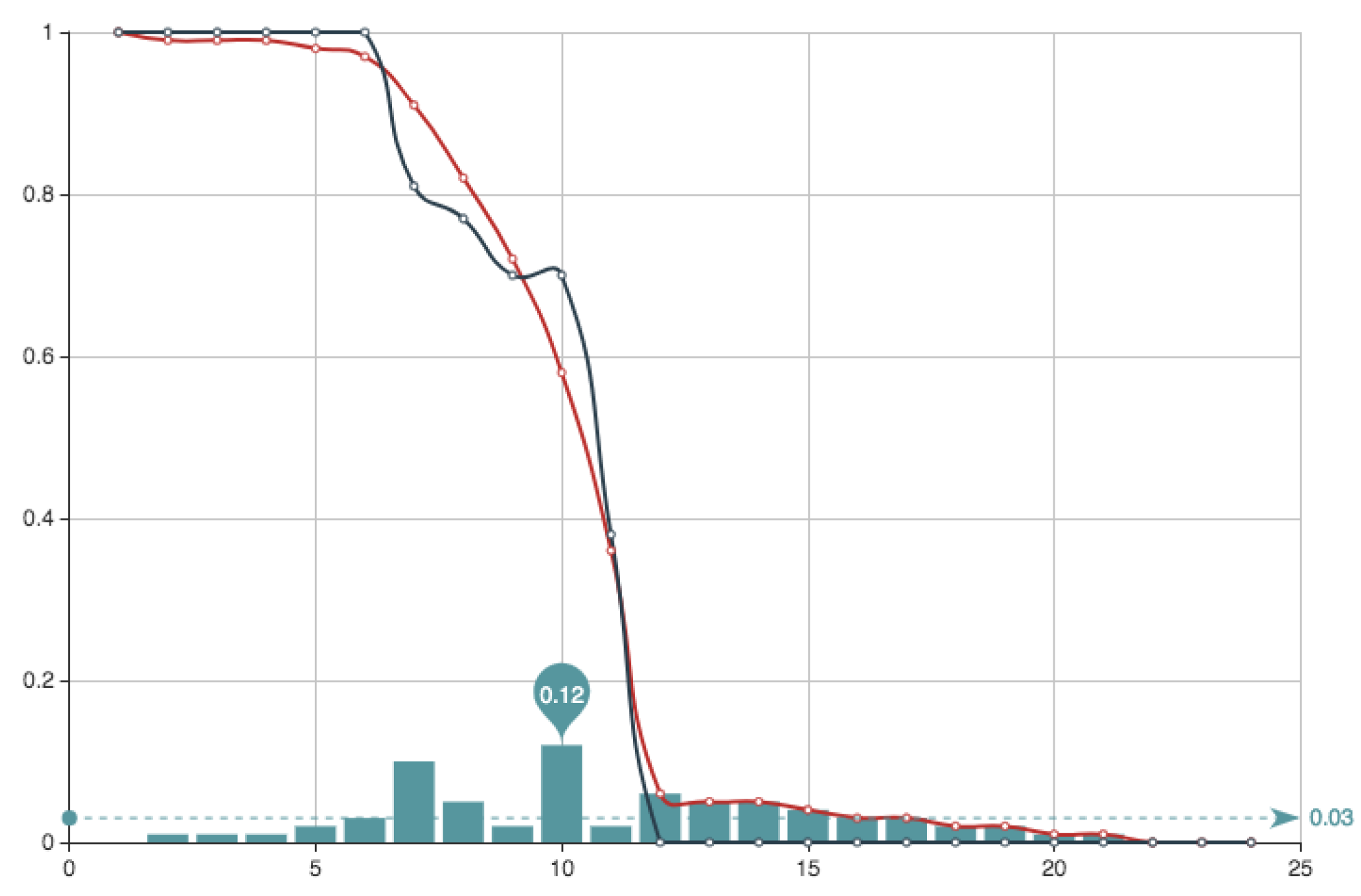
Representation of function E consisting of cumulative recovered individuals plus the dead (black line) and its Monte Carlo approximation (red line). The bar graph is the pointwise error with the maximum (red point) and the average (dashed line).
Figure 4.
Representation of function E consisting of cumulative recovered individuals plus the dead (black line) and its Monte Carlo approximation (red line). The bar graph is the pointwise error with the maximum (red point) and the average (dashed line).

Figure 5.
Joint representation of the data in E (red line) and its approximation for the restriction case (black line). The bar graph is the pointwise error with the maximum (red point) and the average (dashed line).
Figure 5.
Joint representation of the data in E (red line) and its approximation for the restriction case (black line). The bar graph is the pointwise error with the maximum (red point) and the average (dashed line).

Figure 6.
Joint representation of the data in E (red line) and its approximation for the restriction case (black line). The bar graph is the pointwise error with the maximum (red point) and the average (dashed line).
Figure 6.
Joint representation of the data in E (red line) and its approximation for the restriction case (black line). The bar graph is the pointwise error with the maximum (red point) and the average (dashed line).

Figure 7.
Representation of the survival function estimates for the three methods. The red line is the crude Monte Carlo estimate (big Error 422.7197), the black one is the genetic algorithm result, and the red one is the exact approximation based on the Karush-Kuhn-Tucker conditions. The errors for this last/better method are 89.7183—when the constraint is assumed, and 131.0098 for the case
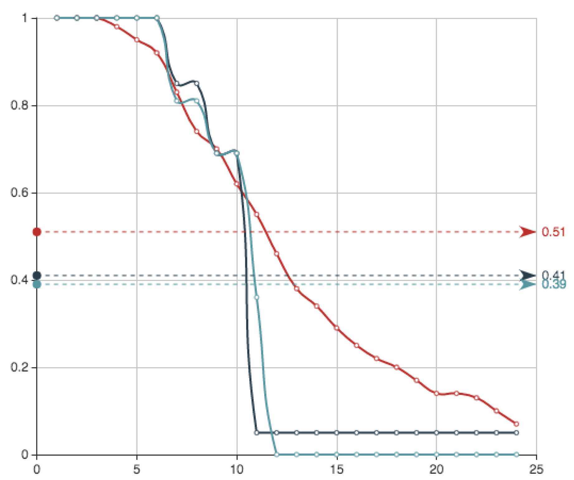
Figure 8.
Joint representation of data and fitting using genetic algorithms.

Figure 9.
Survival function using genetic algorithms.


Table 1.
Main variables used in the model.
| number of new infections at time s | |
| number of death patients at that time s | |
| number of patients considered recovered at time s |
Table 2.
Data record of infected people and the dead of the first 24 days of the Covid-19 epidemics in Spain (natural order from left to right). Data-source: https://github.com/datadista/datasets/tree/master/COVID%2019.
Table 2.
Data record of infected people and the dead of the first 24 days of the Covid-19 epidemics in Spain (natural order from left to right). Data-source: https://github.com/datadista/datasets/tree/master/COVID%2019.
| Infected | 16 | 12 | 22 | 48 | 36 | 48 | 39 | 128 | 65 | 159 | 410 | 623 |
| 506 | 822 | 1259 | 1544 | 2000 | 1438 | 1987 | 2538 | 3431 | 2833 | 4946 | 3646 | |
| Dead | 0 | 0 | 0 | 0 | 0 | 2 | 2 | 3 | 9 | 0 | 18 | 12 |
| 37 | 36 | 16 | 152 | 21 | 182 | 107 | 169 | 235 | 324 | 394 | 462 |
Table 3.
Simulation of the recovered patients provided by the function (natural order from left to right).
Table 3.
Simulation of the recovered patients provided by the function (natural order from left to right).
| Recoreverd | 0 | 0 | 0 | 0 | 0 | 0 | 0 | 0 | 0 | 0.62 | 1.08 | 1.87 |
| 3.23 | 5.54 | 9.48 | 16.17 | 27.54 | 46.85 | 79.61 | 135.15 | 229.31 | 478 | 540 | 450 |
Table 4.
Cumulative sum of the addition of the recovered individuals and the dead (natural order from left to right).
Table 4.
Cumulative sum of the addition of the recovered individuals and the dead (natural order from left to right).
| Recovered and Dead | 0 | 0 | 0 | 0 | 0 | 2 | 4 | 7 |
| 16 | 16.62 | 35.7 | 49.58 | 89.8 | 131.34 | 156.82 | 324.99 | |
| 373.54 | 602.39 | 789 | 1093.15 | 1557.46 | 2359.46 | 3293.46 | 4205.46 |
Table 5.
Exponent in the random sampling and associated error.
| expo | 1 | 5 | 10 |
| Error | 454.0506 | 431.0416 | 422.7197 |
Table 6.
Coefficients for the best MC solution (natural order from left to rigth).
| 0.0005 | 0.0013 | 0.0029 | 0.0150 | 0.0288 | 0.02970 | 0.0936 | 0.0865 |
| 0.0403 | 0.0781 | 0.0707 | 0.0877 | 0.0875 | 0.0328 | 0.0547 | 0.0404 |
| 0.0259 | 0.0227 | 0.0326 | 0.0322 | 0.0004 | 0.0048 | 0.0273 | 0.0304 |
Table 7.
First 12 coefficients of the survival functions for the cases and (the remaining coefficients are 0).
Table 7.
First 12 coefficients of the survival functions for the cases and (the remaining coefficients are 0).
| 0 | 0 | 0.0046 | 0 | 0 | 0 | 0.1492 | 0 | 0.1535 | 0 | 0.6395 | 0 | |
| 0 | 0.0013 | 0 | 0 | 0 | 0 | 0.1903 | 0 | 0.1216 | 0 | 0.3313 | 0.3555 |
Table 8.
Relative error between the exact (Section 3.2) and the approximated solution using GAin terms of the maximum number of iterations and the population size.
Table 8.
Relative error between the exact (Section 3.2) and the approximated solution using GAin terms of the maximum number of iterations and the population size.
| maxiter | ||||
| popSize | 5000 | 25,000 | 50,000 | 100,000 |
| 100 | ||||
| 250 | ||||
| 500 | ||||
© 2020 by the authors. Licensee MDPI, Basel, Switzerland. This article is an open access article distributed under the terms and conditions of the Creative Commons Attribution (CC BY) license (http://creativecommons.org/licenses/by/4.0/).
Share and Cite
MDPI and ACS Style
Calabuig, J.M.; García-Raffi, L.M.; García-Valiente, A.; Sánchez-Pérez, E.A. Evolution Model for Epidemic Diseases Based on the Kaplan-Meier Curve Determination. Mathematics 2020, 8, 1260. https://doi.org/10.3390/math8081260
AMA Style
Calabuig JM, García-Raffi LM, García-Valiente A, Sánchez-Pérez EA. Evolution Model for Epidemic Diseases Based on the Kaplan-Meier Curve Determination. Mathematics. 2020; 8(8):1260. https://doi.org/10.3390/math8081260
Chicago/Turabian StyleCalabuig, Jose M., Luis M. García-Raffi, Albert García-Valiente, and Enrique A. Sánchez-Pérez. 2020. "Evolution Model for Epidemic Diseases Based on the Kaplan-Meier Curve Determination" Mathematics 8, no. 8: 1260. https://doi.org/10.3390/math8081260
Note that from the first issue of 2016, this journal uses article numbers instead of page numbers. See further details here.