Similarity Measure of Lattice Ordered Multi-Fuzzy Soft Sets Based on Set Theoretic Approach and Its Application in Decision Making

Abstract

Many effective tools in fuzzy soft set theory have been proposed to handle various complicated problems in different fields of our real life, especially in decision making. Molodtsov’s soft set theory has been regarded as a newly emerging mathematical tool to deal with uncertainty and vagueness. Lattice ordered multi-fuzzy soft set ($\mathcal{L}\mathcal{M}\mathcal{F}\mathcal{S}\mathcal{S}$) has been applied in forecasting process. However, similarity measure is not used in this application. In our research, similarity measure of $\mathcal{L}\mathcal{M}\mathcal{F}\mathcal{S}\mathcal{S}$ is proposed to calculate the similarity between two $\mathcal{L}\mathcal{M}\mathcal{F}\mathcal{S}\mathcal{S}s$. Moreover, some of its properties are introduced and proved. Finally, an application of $\mathcal{L}\mathcal{M}\mathcal{F}\mathcal{S}\mathcal{S}$ in decision making using similarity measure is analysed.

1. Introduction

Lattice theory plays an important role in many fields in everyday life. The notion of lattices was introduced by Richard Dedekind. Further, Garrett Birrkhoff [1] started the general development of lattice theory in the mid 1930s. George Gratzer [2] vitally developed the theory of lattices and discussed about the applications of lattice theory. In 1965, the notion of fuzzy set was introduced by Zadeh [3] to handle uncertainty in various fields of everyday life. Fuzzy set theory is the generalization of classical set theory, whose range values are within the integer 0 and 1 to the interval [0, 1]. Many researchers such as Xu et al., Roy et al., Majumdar and Samanta, Tripathy et al., are attracted by the concept of fuzzy sets and they have developed new notions of fuzzy sets and applied them in many fields of science and technology, economics, medical science. There are several types of fuzzy set extensions in fuzzy set theory, including intuitionistic fuzzy set, interval-valued fuzzy set, vague set, picture fuzzy set and complex fuzzy set.

In real world complicated problems in engineering, social science, economics, medical science, … classical mathematics methods are always not successful because uncertainty is always present in these problems. A wide range of existing theories such as fuzzy set theory and it extensions in decision making [4], sensitivity analysis in MCDM problems [5], rough set theory in forecasting [6], probability theory, vague set theory and interval mathematics are well known. Apart from that, mathematical approaches are useful to model vagueness. Each of these concepts has its inherent difficulties as pointed out in Reference [7].

In 1999, Molodtsov initiated a new concept of soft set theory, which can be seen as a novel mathematical tool for dealing with uncertainty which is free from the limitations. This theory is useful in different fields such as decision making, data analysis and forecasting and so forth. The soft set model can be combined with other mathematical models. Maji et al. [8] presented the concept of generalized fuzzy soft set theory, which is based on a combination of the fuzzy set and soft set theory. In addition, this concept has proven to be very useful in many different fields. One of the most common applications of soft set is decision making support. Tran Thi Ngan et al. [9] proposed fuzzy aggregation operators and constructed a dental disease diagnosis from X-ray images using these proposed operators. Tran Manh Tuan et al. [10] introduced similarity measure extensions in fuzzy and neutrosophic sets. These measures were implemented in predicting linkage in a co-authorship network with higher performance. Complex fuzzy sets were used in multi-criteria decision making problems [11]. Complex fuzzy t-norms and t-conorms were introduced in this research and applied in solving decision making problem. The complex fuzzy measures on Mamdani complex fuzzy inference systems (Mamdani CFIS) were also presented in Reference [12]. Mamdani fuzzy inference system was extended on complex fuzzy sets. By experimenting on different data sets, Mamdani CFIS worked better comparing with Adaptive Neuro Complex Fuzzy Inference System(ANFIS) and Mamdani Fuzzy Inference System (FIS).

Sebastian and Ramakrishnan [13] proposed the concept of multi-fuzzy sets theory, which is a more general fuzzy set using ordinary fuzzy sets as building blocks and its membership function is an ordered sequence of ordinary fuzzy membership functions. In Reference [14], the notion of multi-fuzzy sets provides a new method to represent some problems which are difficult to explain in other extensions of fuzzy set theory, such as color of pixels. Yong et al. [15] introduced the concept of multi-fuzzy soft set by combining the multi-fuzzy set and soft set models and provided its application in decision making under an imprecise environment. Afterwards, Dey and Pal [16] generalized the notion of multi-fuzzy soft set and its application to decision making.

Similarity measure is an important topic for dealing with uncertain data. In recent years, many researchers have introduced different similarity measures between fuzzy sets, vague sets, soft sets, fuzzy soft sets, intuitionistic fuzzy sets and intuitionistic fuzzy soft sets. Similarity measures have been extensively studied from many aspects and applied in different fields such as decision making, pattern recognition, region extraction, coding theory, image processing, signal detection, security verification systems, medical diagnosis and so on. In 2008, Majumdar and Samanta [17] initiated the study of uncertainty measures of soft sets and also introduced some new similarity measures for fuzzy soft sets, which is based on distance, set theoretic approach and matching function in Reference [18]. Liu et al. [19] proposed similarity measures and entropy of fuzzy soft sets and its properties. Feng and Zheng [20] studied new similarity measures for fuzzy soft sets based on distance measures.

Many various similarity measures on fuzzy sets (FS) were proposed. Peng [21] proposed similarity and distance measure on Pythagorean FS (PFS). These new measures overcame the limitations of introduced similarity or distance measures. This was prove by examples and application in pattern recognition. Fei et al. [22] introduced a novel vector valued similarity measure between two intuitionistic fuzzy sets (IFS). This measure included the uncertainty and similarity for intuitionistic fuzzy sets. This measure was applied in solving classification problem on Iris dataset from UCI. The uncertainty supported the classification when the similarity between two classes was the same. Song et al. [23] reviewed available similarity measures and proposed a similarity measure on IFS based on the functions of IFS (membership, non-membership and hesitation functions). The application on medical data set showed the advantages of proposed measure comparing with other presented ones. The similarity measure on complex multi-fuzzy soft set was presented in Reference [24]. This measure was used to evaluate the alternatives in order to make accuracy decision.

Not only measure the similarity among fuzzy sets, other similarity measures on different objects were also constructed. Chenlei Lv et al. [25] defined a measure to calculate nasal similarity among faces in 3D space. This measure was mainly based on the shape comparison, it was applied into facial classification and identification via a hierarchical structure on public facial datasets. To define users with the same behavior in recommender system based on collaborative filtering, a similarity measure was introduced by Gazdar and Hidri [26]. By experimental results on three UCI data sets, proposed similarity measure obtained higher performance in accuracy and ranking-oriented metrics. Tran Manh Tuan et al. [27] proposed complex fuzzy similarity measures and their weighted versions. These similarity measures were applied in a new rule reduction in order to construct an effective decision making support system.

In 2014, Zhang and Shu [28] extended the idea of multi-fuzzy soft set and introduced the notion of possibility multi-fuzzy soft set and applied it to a decision making problem and also discussed the similarity between two possibility multi-fuzzy soft set and its application to medical diagnosis. Yousef Al-Qudah and Nasruddin Hassan introduced axiomatic definitions of entropy and similarity measure for Complex multi-fuzzy soft set in Reference [24]. Selvachandran et al. proposed distance and distance induced intuitionistic entropy measures for the generalized intuitionistic fuzzy soft set model in Reference [29]. The information measures of distance and similarity for the complex vague soft set model was introduced by Selvachandran et al. in References [30,31] respectively. Vimala et al. initiated new theories such as fuzzy lattice ordered group [32], anti-lattice ordered fuzzy soft group [33], lattice ordered interval-valued hesitant fuzzy soft sets [34] and applied it to decision making problems [35] and also introduced the new concept of complex intuitionistic fuzzy soft lattice ordered group and its weighted distance measures in Reference [36]. Further, Sabeena begam et al. [37] derived the concept of lattice approach on multi-fuzzy soft set and also illustrated its application using forecasting process. The similarity measure between two $\mathcal{L}\mathcal{M}\mathcal{F}\mathcal{S}\mathcal{S}s$ was not proposed. Later, the algebraic aspects of $\mathcal{L}\mathcal{M}\mathcal{F}\mathcal{S}\mathcal{S}$ such as new concept of modular and distributive $\mathcal{L}\mathcal{M}\mathcal{F}\mathcal{S}\mathcal{S}$ were presented in Reference [38]. Its properties were also established.

The main purpose of this paper is to introduce the concept of similarity between two lattice ordered multi-fuzzy soft sets. This is a new similarity measure between two $\mathcal{L}\mathcal{M}\mathcal{F}\mathcal{S}\mathcal{S}s$. To illustrate the proposed measure, two numerical examples are performed step by step. Our proposed fuzzy similarity measure has some main advantages. Firstly, this measure is simple and very efficient to evaluate. Secondly, this measure is introduced in multi-dimension using the lattice structure that makes it be easier for explanation in many problems. The properties of proposed measure and an application in decision making using this measure are also presented. Although the good properties of a similarity measure between two vectors were pointed out in Reference [39]. But in this paper, we are checking the similarity measure based on soft set theory. Thus, properties mentioned in Reference [39] were not suitable to evaluate our measure.

This paper is organized as follows—in Section 2, fundamentals of fuzzy set theory, soft set theory, fuzzy soft set theory, multi-fuzzy set theory, multi-fuzzy soft set theory, $\mathcal{L}\mathcal{M}\mathcal{F}\mathcal{S}\mathcal{S}$ and its operations which are useful for subsequent discussions are presented. Novel similarity measures between two $\mathcal{L}\mathcal{M}\mathcal{F}\mathcal{S}\mathcal{S}s$ are discussed in Section 3. Section 4 discusses the application of similarity measures in two $\mathcal{L}\mathcal{M}\mathcal{F}\mathcal{S}\mathcal{S}s$. In Section 5, some conclusions and further works are provided.

2. Preliminaries

In this section, we summarize some of the important concepts related to this paper pertaining to soft set, multi-fuzzy set, multi-fuzzy soft set and lattice ordered multi-fuzzy soft set.

2.1. Fuzzy Sets and Fuzzy Soft Sets

Fuzzy set is a type of very important mathematical structure to represent a collection of objects whose boundary is vague.

Definition 1

([3]). Let U be a non-empty set. Let $A=\left\{\right(x,\mu \left(x\right)):x\in U\}$ with $\mu :U⟶[0,1]$. Then A is said to be a fuzzy set over U, and μ is said to be the membership function of A.

Denote the power set of U by $\wp \left(U\right)$. Molodtsov defined the concept of a soft set in the following way:

Definition 2

([7]). Let U be a non-empty set. Let E be a set of parameters. Let $\mathcal{G}:E⟶\wp \left(U\right)$. Then $(\mathcal{G},E)=\left\{\right(\epsilon ,\mathcal{G}\left(\epsilon \right)):\epsilon \in E\}$ is said to be a soft set on U. In particular, $\mathcal{G}\left({\epsilon }_0\right)$ is said to be the set of ${\epsilon }_0$-approximate elements of $(\mathcal{G},E)$.

Denote the collection of all the fuzzy sets (as defined in Definition 1) over U by $\mathcal{F}\left(U\right)$. Maji described the concept of fuzzy soft set in the following manner:

Definition 3

([8]). Let U be a non-empty set. Let E be a set of parameters. Let $\mathcal{H}:E⟶\mathcal{F}\left(U\right)$. Then $(\mathcal{H},E)=\left\{\right(\epsilon ,\mathcal{H}\left(\epsilon \right)):\epsilon \in E\}$ is said to be a fuzzy soft set on U. In particular, $\mathcal{H}\left({\epsilon }_0\right)$ is said to be the fuzzy set of ${\epsilon }_0$-approximate elements of $(\mathcal{H},E)$.

2.2. Multi-Fuzzy Sets and Multi-Fuzzy Soft Sets

In 2011, the concept of fuzzy sets was generalized to multi-fuzzy sets by Sebastian and Ramakrishnan. Multi-fuzzy set theory as a mathematical tool to deal with life problems that have multi-dimensional characterization properties.

Definition 4

([13]). Let U be a non-empty set. Let J be a set of indices. Let

$$\tilde{A}=\{\left(x,{\left({\mu }_j\left(x\right)\right)}_{j\in J}\right):x\in U\},$$

(1)

with ${\mu }_j:U⟶[0,1]$ for all $j\in J$. Then

i. 

$\tilde{A}$ is said to be a multi-fuzzy set in U.

ii. 

J is said to be the index of $\tilde{A}$.

iii. 

$\left|J\right|$ is said to be the dimension of $\tilde{A}$.

iv. 

${\left({\mu }_j\right)}_{j\in J}$ is said to be the multi-membership function of $\tilde{A}$.

Remark 1.

For the particular case of $J=\left\{1,2,\dots ,p\right\}\subset \mathbb{N}$ in Definition 4:

i. 

${\left({\mu }_j\left(x\right)\right)}_{j\in J}=({\mu }_1\left(x\right),{\mu }_2\left(x\right),\dots ,{\mu }_p\left(x\right))$.

ii. 

${\left({\mu }_j\right)}_{j\in J}=({\mu }_1,{\mu }_2,\dots ,{\mu }_p)$.

iii. 

$\left|J\right|=p$.

The collection of all multi-fuzzy sets in U shall be denoted as $\mathcal{M}\mathcal{F}\mathcal{S}\left(U\right)$. In particular, of all multi-fuzzy sets in U with the index J shall be denoted as $\mathcal{M}{\mathcal{F}}_J\mathcal{S}\left(U\right)$.

Definition 5

([14]). Let U be a non-empty set. Let $\tilde{A},\tilde{B}\in \mathcal{M}\mathcal{F},\mathcal{S}\left(U\right)$ which both have the same index J. Denote ${\left({\mu }_j\right)}_{j\in J}$ and ${\left({\nu }_j\right)}_{j\in J}$ to be the multi-membership functions of $\tilde{A}$ and $\tilde{B}$ respectively. Then, $\tilde{A}$ is said to be a multi-fuzzy subset of $\tilde{B}$, denoted as $\tilde{A}⊑\tilde{B}$, if ${\mu }_j\left(x\right)⩽{\nu }_j\left(x\right)$ for all $j\in J$ and for all $x\in U$.

In other words, the relationship of multi-fuzzy subset is only defined among multi-fuzzy sets sharing the same index. As a result, whenever given $\tilde{P}⊑\tilde{Q}$, it is well understood that $\tilde{P}$ and $\tilde{Q}$ must have the same index.

Definition 6

([14]). Let U be a non-empty set. Let $\tilde{A},\tilde{B}\in \mathcal{M}\mathcal{F}\mathcal{S}\left(U\right)$. $\tilde{A}$ and $\tilde{B}$ are said to be equal, denoted as $\tilde{A}=\tilde{B}$, if both $\tilde{A}⊑\tilde{B}$ and $\tilde{B}⊑\tilde{A}$ holds.

Definition 7

([14]). Let U be a non-empty set. Let $\tilde{A},\tilde{B}\in \mathcal{M}\mathcal{F}\mathcal{S}\left(U\right)$ which both have the same index J. Denote ${\left({\mu }_j\right)}_{j\in J}$ and ${\left({\nu }_j\right)}_{j\in J}$ to be the multi-membership functions of $\tilde{A}$ and $\tilde{B}$ respectively. The union and intersection of $\tilde{A}$ and $\tilde{B}$, denoted as $\tilde{A}\bigsqcup \tilde{B}$ and $\tilde{A}\sqcap \tilde{B}$ respectively, is defined to be the following multi-fuzzy sets in U:

$$\tilde{A}\bigsqcup \tilde{B}=\{\left(x,{\left(max\{{\mu }_j\left(x\right),{\nu }_j\left(x\right)\}\right)}_{j\in J}\right):x\in U\}$$

(2)

$$\tilde{A}\sqcap \tilde{B}=\{\left(x,{\left(min\{{\mu }_j\left(x\right),{\nu }_j\left(x\right)\}\right)}_{j\in J}\right):x\in U\}.$$

(3)

Yang et al. initiated multi-fuzzy soft set, which can be seen as an extension of multi-fuzzy set and soft set model. It is defined as follows:

Definition 8

([15]). Let U be a non-empty set. Let E be a set of parameters. Let $\tilde{\mathcal{F}}:E⟶\mathcal{M}\mathcal{F}\mathcal{S}\left(U\right)$. Then $(\tilde{\mathcal{F}},E)=\{(\epsilon ,\tilde{\mathcal{F}}\left(\epsilon \right)):\epsilon \in E\}$ is said to be a multi-fuzzy soft set on U.

The collection of all multi-fuzzy soft sets on U shall be denoted as $\mathcal{M}\mathcal{F}\mathcal{S}\mathcal{S}\left(U\right)$. In particular, the collection of all multi-fuzzy soft sets on U with index in J shall be denoted as $\mathcal{M}{\mathcal{F}}_J\mathcal{S}\mathcal{S}\left(U\right)$.

Remark 2.

Given any $\epsilon \in E$ in Definition 8. As $\tilde{\mathcal{F}}\left(\epsilon \right)\in \mathcal{M}\mathcal{F}\mathcal{S}\mathcal{S}\left(U\right)$, $\tilde{\mathcal{F}}\left(\epsilon \right)$ comes with its index $J_{\epsilon }$ by Definition 4. However, $J_{{\epsilon }_1}$ and $J_{{\epsilon }_2}$ need not be equal given any $\{{\epsilon }_1,{\epsilon }_2\}\subseteq E$.

Definition 9

([15]). Let U be a non empty set. Let $A,B$ be two sets of parameters. Let $(\tilde{\mathcal{F}},A),(\tilde{\mathcal{G}},B)\in \mathcal{M}\mathcal{F}\mathcal{S}\mathcal{S}\left(U\right)$. $(\tilde{\mathcal{F}},A)$ is said to be a multi-fuzzy soft subset of $(\tilde{\mathcal{G}},B)$ if

i. 

$A\subseteq B$.

ii. 

$\tilde{\mathcal{F}}\left(\alpha \right)⊑\tilde{\mathcal{G}}\left(\alpha \right)$ for all $\alpha \in A$

In such a case, we write $(\tilde{\mathcal{F}},A)\subseteq (\tilde{\mathcal{G}},B)$.

For ease on notation, the notation of ⊑ used in Reference [14] was not carried forward to Reference [15].

Definition 10

([15]). Let U be a non empty sets. Let $A,B$ be two sets of parameters. Let $(\tilde{\mathcal{F}},A),(\tilde{\mathcal{G}},B)\in \mathcal{M}\mathcal{F}\mathcal{S}\mathcal{S}\left(U\right)$. $(\tilde{\mathcal{F}},A)$ and $(\tilde{\mathcal{G}},B)$ are said to be equal if both $(\tilde{\mathcal{F}},A)\subseteq (\tilde{\mathcal{G}},B)$ and $(\tilde{\mathcal{G}},B)\subseteq (\tilde{\mathcal{F}},A)$ holds. In such a case, we write $(\tilde{\mathcal{F}},A)$ = $(\tilde{\mathcal{G}},B)$.

Definition 11

([15]). The union of $(\tilde{\mathcal{F}},A),(\tilde{\mathcal{G}},B)\in \mathcal{M}\mathcal{F}\mathcal{S}\mathcal{S}\left(U\right)$ is defined to be $(\tilde{\mathcal{H}},C)\in \mathcal{M}\mathcal{F}\mathcal{S}\mathcal{S}\left(U\right)$ where $C=A\cup B$, and with $\tilde{\mathcal{H}}\left(\epsilon \right)$=$\left\{\begin{array}{cc}\tilde{\mathcal{F}}\left(\epsilon \right)\hfill & if\epsilon \in A\backslash B\hfill \\ \tilde{\mathcal{G}}\left(\epsilon \right)\hfill & if\epsilon \in B\backslash A\hfill \\ \tilde{\mathcal{F}}\left(\epsilon \right)\bigsqcup \tilde{\mathcal{G}}\left(e\right)\hfill & if\epsilon \in A\cap B\hfill \end{array}\right.$

for all $\epsilon \in C$.

In such a case, we write $(\tilde{\mathcal{H}},C)=(\tilde{\mathcal{F}},A)\cup (\tilde{\mathcal{G}},B)$.

Definition 12

([15]). The intersection of $(\tilde{\mathcal{F}},A),(\tilde{\mathcal{G}},B)\in \mathcal{M}\mathcal{F}\mathcal{S}\mathcal{S}\left(U\right)$ is defined to be $(\tilde{\mathcal{K}},D)\in \mathcal{M}\mathcal{F}\mathcal{S}\mathcal{S}\left(U\right)$ where $D=A\cap B$, and with $\tilde{\mathcal{K}}\left(\epsilon \right)=\tilde{\mathcal{F}}\left(\epsilon \right)\sqcap \tilde{\mathcal{G}}\left(\epsilon \right)$ for all $\epsilon \in D$.

In such a case, we write $(\tilde{\mathcal{K}},D)=(\tilde{\mathcal{F}},A)\cap (\tilde{\mathcal{G}},B)$.

Definition 13

([15]). The conjunction of $(\tilde{\mathcal{F}},A),(\tilde{\mathcal{G}},B)\in \mathcal{M}\mathcal{F}\mathcal{S}\mathcal{S}\left(U\right)$ is defined to be $(\tilde{\mathcal{L}},P)\in \mathcal{M}\mathcal{F}\mathcal{S}\mathcal{S}\left(U\right)$ where $P=A\times B$, and with $\tilde{\mathcal{L}}(\alpha ,\beta )=\tilde{\mathcal{F}}\left(\alpha \right)\sqcap \tilde{\mathcal{G}}\left(\beta \right)$ for all $(\alpha ,\beta )\in P$.

In such a case, we write $(\tilde{\mathcal{L}},P)=(\tilde{\mathcal{F}},A)\wedge (\tilde{\mathcal{G}},B)$.

Definition 14

([15]). The disjunction of $(\tilde{\mathcal{F}},A),(\tilde{\mathcal{G}},B)\in \mathcal{M}\mathcal{F}\mathcal{S}\mathcal{S}\left(U\right)$ is defined to be $(\tilde{\mathcal{T}},P)\in \mathcal{M}\mathcal{F}\mathcal{S}\mathcal{S}\left(U\right)$ where $P=A\times B$, and with $\tilde{\mathcal{T}}(\alpha ,\beta )=\tilde{\mathcal{F}}\left(\alpha \right)\bigsqcup \tilde{\mathcal{G}}\left(\beta \right)$ for all $(\alpha ,\beta )\in P$.

In such a case, we write $(\tilde{\mathcal{T}},P)=(\tilde{\mathcal{F}},A)\vee (\tilde{\mathcal{G}},B)$.

2.3. Lattice Ordered Multi-Fuzzy Soft Set ($\mathcal{L}\mathcal{M}\mathcal{F}\mathcal{S}\mathcal{S}$)

Throughout this paper, $\tilde{X}$ refers to the initial universe, P($\tilde{X}$) is the power set of $\tilde{X}$, $\tilde{E}$ is a set of parameters and $\tilde{\mathcal{A}}\subseteq \tilde{E}$.

In all the following passages, the concept of the lattice is referred to the one encountered in the literature of partially ordered sets (posets). We now combine the concepts of lattices and multi-fuzzy soft sets to obtain a new hyprid structure called lattice ordered multi-fuzzy soft set.

Definition 15

([37]). Let U be a non-empty set. Let J be a set of indices. Let Λ be a lattice of parameters. Let $\tilde{\mathcal{R}}:\mathsf{\Lambda }⟶\mathcal{M}{\mathcal{F}}_J\mathcal{S}\left(U\right)$ be such that, for all ${\lambda }_1,{\lambda }_2\in \mathsf{\Lambda }$: ${\lambda }_1⩽{\lambda }_2$ implies $\tilde{\mathcal{R}}\left({\lambda }_1\right)⊑\tilde{\mathcal{R}}\left({\lambda }_2\right)$. Then $(\tilde{\mathcal{R}},\mathsf{\Lambda })=\{(\epsilon ,\tilde{\mathcal{R}}\left(\lambda \right)):\lambda \in \mathsf{\Lambda }\}$ is said to be a lattice ordered multi-fuzzy soft set on U with index J.

The collection of all lattice ordered multi-fuzzy soft sets on U with index in J shall be denoted as $\mathcal{L}\mathcal{M}{\mathcal{F}}_J\mathcal{S}\mathcal{S}\left(U\right)$.

Furthermore, the collection of all lattice ordered multi-fuzzy soft sets on U shall be denoted as $\mathcal{L}\mathcal{M}\mathcal{F}\mathcal{S}\mathcal{S}\left(U\right)$. Note that a lattice ordered multi-fuzzy soft set can only be established upon a collection of multi-fuzzy soft sets all sharing a particular index in J. As a result, $\mathcal{L}\mathcal{M}\mathcal{F}\mathcal{S}\mathcal{S}\left(U\right)={\bigcup }_{\mathrm{all}J}\mathcal{L}\mathcal{M}{\mathcal{F}}_J\mathcal{S}\mathcal{S}\left(U\right)$.

Example 1

([37]). There are three international companies in India who manufactures vehicles for the world market, namely x, y and z. Their most frequent buyer is known to be Japan. Besides Japan, they advertise their products mainly to countries of the G20 (due to their economic advancements), as well as countries in Asia (due to geographic closeness). Note that Japan belongs to both G20 and Asia, but none of G20 or Asia fully covers the other.

Thus it is now desired to assess the sales performance of these three companies in four regions—Japan, G20, Asia, and worldwide. The assessment is purely based on the amount of revenue generated and is given as numbers from 0 (no revenue) to 1 (highest revenue). As a result, the wider the region of consideration, the higher the score as more sales take place in that wider region.

On the other hand, as each of these companies manufactures bikes, cars and trucks, the committee agreed to look at these three products separately.

In this example, let the results be summarized as the following tables for each of the 4 regions (

Table 1. Sales performances in Japan.

	Bikes	Cars	Trucks
Company x	0.2	0.3	0.6
Company y	0.5	0.3	0.4
Company z	0.6	0.5	0.3

,

Table 2. Sales performances among countries of the G20.

	Bikes	Cars	Trucks
Company x	0.5	0.4	0.8
Company y	0.5	0.5	0.5
Company z	0.7	0.6	0.5

,

Table 3. Sales performances in Asia.

	Bikes	Cars	Trucks
Company x	0.3	0.5	0.7
Company y	0.6	0.4	0.7
Company z	0.8	0.7	0.4

and

Table 4. Sales performances worldwide.

	Bikes	Cars	Trucks
Company x	0.8	0.6	0.8
Company y	0.7	0.6	0.9
Company z	0.9	0.8	0.6

).

With all of these inputs:

a. 

Denote the 3 companies with the non-empty set $U_0$ = $\{x,y,z\}$.

b. 

Denote the 4 regions with the lattice of parameters ${\mathsf{\Lambda }}_0=\{\alpha =Japan,\beta =G20,\gamma =Asia,\xi =\mathit{worldwide}\}$, for which $\alpha ⩽\beta ⩽\xi$ and $\alpha ⩽\gamma ⩽\xi$, but no such relationship established between β and γ.

c. 

Denote the 3 categories of assessment with the set of indexes $J_0=\{b=\mathit{bike},c=\mathit{car},t=\mathit{truck}\}$. And take ${\left({\mu }_j\right)}_{j\in J_0}=({\mu }_b,{\mu }_c,{\mu }_t)$, thus fixing the order of appearance of the elements of $J_0$ in the presentation of ${\left({\mu }_j\right)}_{j\in J_0}$.

We have thus formed a lattice ordered multi-fuzzy soft set as shown:

$({\tilde{\mathcal{R}}}_0,{\mathsf{\Lambda }}_0)$

$=\{{\tilde{\mathcal{R}}}_0\left(\alpha \right)=\{\frac{x}{(0.2,0.3,0.6)},\frac{y}{(0.5,0.3,0.4)},\frac{z}{(0.6,0.5,0.3)}\}$

${\tilde{\mathcal{R}}}_0\left(\beta \right)=\{\frac{x}{(0.5,0.4,0.8)},\frac{y}{(0.5,0.5,0.5)},\frac{z}{(0.7,0.6,0.5)}\}$

${\tilde{\mathcal{R}}}_0\left(\gamma \right)=\{\frac{x}{(0.3,0.5,0.7)},\frac{y}{(0.6,0.4,0.7)},\frac{z}{(0.8,0.7,0.4)}\}$

${\tilde{\mathcal{R}}}_0\left(\xi \right)=\{\frac{x}{(0.8,0.6,0.8)},\frac{y}{(0.7,0.6,0.9)},\frac{z}{(0.9,0.8,0.6)}\}\}\in \mathcal{L}\mathcal{M}{\mathcal{F}}_{J_0}\mathcal{S}\mathcal{S}\left(U_0\right)\subseteq \mathcal{L}\mathcal{M}\mathcal{F}\mathcal{S}\mathcal{S}\left(U_0\right)$.

3. Similarity between Two $\mathcal{L}\mathcal{M}\mathcal{F}\mathcal{S}\mathcal{S}\mathit{s}$ Based on Set Theoretic Approach

In this section, we introduce the concept of similarity measure of two $\mathcal{L}\mathcal{M}\mathcal{F}\mathcal{S}\mathcal{S}s$ and further results on similarity measure of two $\mathcal{L}\mathcal{M}\mathcal{F}\mathcal{S}\mathcal{S}s$. In all the following context, denote $a\wedge b$ to be the minimum of a and b, denote $a\vee b$ to be the maximum of a and b.

Definition 16.

Let $(\tilde{\mathcal{R}},\mathsf{\Gamma }),(\tilde{\mathcal{Q}},\mathsf{\Gamma })\in \mathcal{L}\mathcal{M}{\mathcal{F}}_J\mathcal{S}\mathcal{S}\left(U\right)$.

The similarity measure of $(\tilde{\mathcal{R}},\mathsf{\Gamma })$ and $(\tilde{\mathcal{Q}},\mathsf{\Gamma })$ over U is defined as

$$\mathbf{S}((\tilde{\mathcal{R}},\mathsf{\Gamma }),(\tilde{\mathcal{Q}},\mathsf{\Gamma }))=\frac{{\sum }_{j\in J}{S}_j((\tilde{\mathcal{R}},\mathsf{\Gamma }),(\tilde{\mathcal{Q}},\mathsf{\Gamma }))}{\left|J\right|}$$

where

$$S_j((\tilde{\mathcal{R}},\mathsf{\Gamma }),(\tilde{\mathcal{Q}},\mathsf{\Gamma }))=\frac{{\sum }_{\gamma \in \mathsf{\Gamma }}{\vee }_{x\in U}\{{\mu }_{\tilde{\mathcal{R}}\left(\gamma \right),j}\left(x\right)\wedge {\mu }_{\tilde{\mathcal{Q}}\left(\gamma \right),j}\left(x\right)\}}{{\sum }_{\gamma \in \mathsf{\Gamma }}{\vee }_{x\in U}\{{\mu }_{\tilde{\mathcal{R}}\left(\gamma \right),j}\left(x\right)\vee {\mu }_{\tilde{\mathcal{Q}}\left(\gamma \right),j}\left(x\right)\}}$$

Example 2.

Let $U_0=\{x_1,x_2,x_3,x_4\}$. Let $J_0=\{1,2,3\}$.

Let ${\mathsf{\Gamma }}_0=\{{\gamma }_1,{\gamma }_2,{\gamma }_3,{\gamma }_4\}$, for which ${\gamma }_1⩽{\gamma }_2⩽{\gamma }_3⩽{\gamma }_4$.

Let $({\tilde{\mathcal{R}}}_0,{\mathsf{\Gamma }}_0),({\tilde{\mathcal{Q}}}_0,{\mathsf{\Gamma }}_0)\in \mathcal{L}\mathcal{M}{\mathcal{F}}_{J_0}\mathcal{S}\mathcal{S}\left(U_0\right)$ which are defined as follows:

$({\tilde{\mathcal{R}}}_0,{\mathsf{\Gamma }}_0)=\{{\tilde{\mathcal{R}}}_0\left({\gamma }_1\right)=\{\frac{x_1}{(0.2,0.1,0.3)},\frac{x_2}{(0.1,0.2,0.4)},\frac{x_3}{(0.18,0.23,0.45)},\frac{x_4}{(0.3,0.6,0.2)}\}$,

${\tilde{\mathcal{R}}}_0\left({\gamma }_2\right)=\{\frac{x_1}{(0.28,0.49,0.5)},\frac{x_2}{(0.33,0.42,0.63)},\frac{x_3}{(0.29,0.33,0.52)},\frac{x_4}{(0.4,0.68,0.3)}\}$,

${\tilde{\mathcal{R}}}_0\left({\gamma }_3\right)=\{\frac{x_1}{(0.6,0.72,0.69)},\frac{x_2}{(0.47,0.73,0.8)},\frac{x_3}{(0.5,0.62,0.8)},\frac{x_4}{(0.5,0.7,0.4)}\}$,

${\tilde{\mathcal{R}}}_0\left({\gamma }_4\right)=\{\frac{x_1}{(0.8,0.85,0.93)},\frac{x_2}{(0.52,0.8,0.9)},\frac{x_3}{(0.6,0.7,0.9)},\frac{x_4}{(0.7,0.9,1.0)}\}\}$

and

$({\tilde{\mathcal{Q}}}_0,{\mathsf{\Gamma }}_0)=\{{\tilde{\mathcal{Q}}}_0\left({\gamma }_1\right)=\{\frac{x_1}{(0.1,0.4,0.2)},\frac{x_2}{(0.3,0.1,0.2)},\frac{x_3}{(0.2,0.1,0.3)},\frac{x_4}{(0.1,0.4,0.3)}\}$,

${\tilde{\mathcal{Q}}}_0\left({\gamma }_2\right)=\{\frac{x_1}{(0.23,0.5,0.4)},\frac{x_2}{(0.4,0.25,0.36)},\frac{x_3}{(0.32,0.4,0.5)},\frac{x_4}{(0.32,0.5,0.4)}\}$,

${\tilde{\mathcal{Q}}}_0\left({\gamma }_3\right)=\{\frac{x_1}{(0.43,0.8,0.7)},\frac{x_2}{(0.5,0.6,0.7)},\frac{x_3}{(0.4,0.71,0.6)},\frac{x_4}{(0.4,0.62,0.5)}\}$,

${\tilde{\mathcal{Q}}}_0\left({\gamma }_4\right)=\{\frac{x_1}{(0.7,0.82,1.0)},\frac{x_2}{(0.8,0.75,1.0)},\frac{x_3}{(0.8,0.9,0.95)},\frac{x_4}{(0.8,0.7,0.6)}\}\}$.

where ${\left({\mu }_j\right)}_{j\in J_0}=({\mu }_{j_1},{\mu }_{j_2},{\mu }_{j_3})$.

By Definition 16, we obtain,

$$\begin{array}{cc}& S_1((\tilde{\mathcal{R}},\mathsf{\Gamma }),(\tilde{\mathcal{Q}},\mathsf{\Gamma }))=\hfill \\ =& \frac{{\sum }_{\gamma \in \mathsf{\Gamma }}{\vee }_{x\in U}\{{\mu }_{\tilde{\mathcal{R}}\left(\gamma \right),j_1}\left(x\right)\wedge {\mu }_{\tilde{\mathcal{Q}}\left(\gamma \right),j_1}\left(x\right)\}}{{\sum }_{\gamma \in \mathsf{\Gamma }}{\vee }_{x\in U}\{{\mu }_{\tilde{\mathcal{R}}\left(\gamma \right),j_1}\left(x\right)\vee {\mu }_{\tilde{\mathcal{Q}}\left(\gamma \right),j_1}\left(x\right)\}}\hfill \\ =& \frac{(0.1\vee 0.1\vee 0.18\vee 0.1)+(0.23\vee 0.33\vee 0.29\vee 0.32)+(0.43\vee 0.47\vee 0.4\vee 0.4)+(0.7\vee 0.52\vee 0.6\vee 0.7)}{0.2\vee 0.3\vee 0.2\vee 0.3+0.28\vee 0.4\vee 0.32\vee 0.4+0.6\vee 0.5\vee 0.5\vee 0.5+0.8\vee 0.8\vee 0.8\vee 0.8}\hfill \\ =& \frac{0.8+0.33+0.47+0.7}{0.3+0.4+0.6+0.8}\hfill \\ =& 0.8\hfill \end{array}$$

$$\begin{array}{cc}& S_2((\tilde{\mathcal{R}},\mathsf{\Gamma }),(\tilde{\mathcal{Q}},\mathsf{\Gamma }))=\hfill \\ =& \frac{{\sum }_{\gamma \in \mathsf{\Gamma }}{\vee }_{x\in U}\{{\mu }_{\tilde{\mathcal{R}}\left(\gamma \right),j_2}\left(x\right)\wedge {\mu }_{\tilde{\mathcal{Q}}\left(\gamma \right),j_2}\left(x\right)\}}{{\sum }_{\gamma \in \mathsf{\Gamma }}{\vee }_{x\in U}\{{\mu }_{\tilde{\mathcal{R}}\left(\gamma \right),j_2}\left(x\right)\vee {\mu }_{\tilde{\mathcal{Q}}\left(\gamma \right),j_2}\left(x\right)\}}\hfill \\ =& \frac{(0.1\vee 0.1\vee 0.1\vee 0.4)+(0.49\vee 0.25\vee 0.33\vee 0.5)+(0.72\vee 0.6\vee 0.62\vee 0.62)+(0.82\vee 0.75\vee 0.7\vee 0.7)}{0.4\vee 0.2\vee 0.23\vee 0.6+0.5\vee 0.42\vee 0.4\vee 0.68+0.8\vee 0.73\vee 0.71\vee 0.7+0.85\vee 0.8\vee 0.9\vee 0.9}\hfill \\ =& \frac{0.4+0.5+0.72+0.82}{0.6+0.68+0.8+0.9}\hfill \\ =& 0.82\hfill \end{array}$$

$$\begin{array}{cc}& S_3((\tilde{\mathcal{R}},\mathsf{\Gamma }),(\tilde{\mathcal{Q}},\mathsf{\Gamma }))=\hfill \\ =& \frac{{\sum }_{\gamma \in \mathsf{\Gamma }}{\vee }_{x\in U}\{{\mu }_{\tilde{\mathcal{R}}\left(\gamma \right),j_3}\left(x\right)\wedge {\mu }_{\tilde{\mathcal{Q}}\left(\gamma \right),j_3}\left(x\right)\}}{{\sum }_{\gamma \in \mathsf{\Gamma }}{\vee }_{x\in U}\{{\mu }_{\tilde{\mathcal{R}}\left(\gamma \right),j_3}\left(x\right)\vee {\mu }_{\tilde{\mathcal{Q}}\left(\gamma \right),j_3}\left(x\right)\}}\hfill \\ =& \frac{(0.2\vee 0.2\vee 0.3\vee 0.2)+(0.4\vee 0.36\vee 0.5\vee 0.3)+(0.69\vee 0.7\vee 0.6\vee 0.4)+(0.93\vee 0.9\vee 0.9\vee 0.6)}{0.3\vee 0.4\vee 0.45\vee 0.3+0.5\vee 0.63\vee 0.52\vee 0.4+0.7\vee 0.8\vee 0.8\vee 0.5+1.0\vee 1.0\vee 0.95\vee 1.0}\hfill \\ =& \frac{0.3+0.5+0.7+0.93}{0.45+0.63+0.8+1.0}\hfill \\ =& 0.84\hfill \end{array}$$

Then the similarity between $({\tilde{\mathcal{R}}}_0,{\mathsf{\Gamma }}_0)$ and $({\tilde{\mathcal{Q}}}_0,{\mathsf{\Gamma }}_0)$ over $U_0$ is thus

$\mathbf{S}(({\tilde{\mathcal{R}}}_0,{\mathsf{\Gamma }}_0),({\tilde{\mathcal{Q}}}_0,{\mathsf{\Gamma }}_0))=\frac{{\sum }_{j\in J_0}{S}_j(({\tilde{\mathcal{R}}}_0,{\mathsf{\Gamma }}_0),({\tilde{\mathcal{Q}}}_0,{\mathsf{\Gamma }}_0))}{|J_0|}=\frac{0.80+0.82+0.84}{3}=0.82$.

Theorem 1.

Let $(\tilde{\mathcal{R}},\mathsf{\Gamma }),(\tilde{\mathcal{Q}},\mathsf{\Gamma }),(\tilde{\mathcal{P}},\mathsf{\Gamma })\in \mathcal{L}\mathcal{M}{\mathcal{F}}_J\mathcal{S}\mathcal{S}\left(U\right)$. Then the following holds:

i. 

$\mathbf{S}((\tilde{\mathcal{R}},\mathsf{\Gamma }),(\tilde{\mathcal{Q}},\mathsf{\Gamma }))=\mathbf{S}((\tilde{\mathcal{Q}},\mathsf{\Gamma }),(\tilde{\mathcal{R}},\mathsf{\Gamma }))$.

ii. 

$0\le \mathbf{S}((\tilde{\mathcal{R}},\mathsf{\Gamma }),(\tilde{\mathcal{Q}},\mathsf{\Gamma }))\le 1$.

iii. 

$\mathbf{S}((\tilde{\mathcal{R}},\mathsf{\Gamma }),(\tilde{\mathcal{Q}},\mathsf{\Gamma }))=1\Rightarrow (\tilde{\mathcal{R}},\mathsf{\Gamma })=(\tilde{\mathcal{Q}},\mathsf{\Gamma })\ne \varnothing$

iv. 

$\mathbf{S}((\tilde{\mathcal{R}},\mathsf{\Gamma }),(\tilde{\mathcal{Q}},\mathsf{\Gamma }))=0\Rightarrow (\tilde{\mathcal{R}},\mathsf{\Gamma })\cap (\tilde{\mathcal{Q}},\mathsf{\Gamma })=\varnothing$.

v. 

$(\tilde{\mathcal{R}},\mathsf{\Gamma })\subseteq (\tilde{\mathcal{Q}},\mathsf{\Gamma })\subseteq (\tilde{\mathcal{P}},\mathsf{\Gamma })\Rightarrow \mathbf{S}((\tilde{\mathcal{R}},\mathsf{\Gamma }),(\tilde{\mathcal{P}},\mathsf{\Gamma }))\le \mathbf{S}((\tilde{\mathcal{Q}},\mathsf{\Gamma }),(\tilde{\mathcal{P}},\mathsf{\Gamma }))$.

Proof. 

(i) For

$$\begin{array}{ccc}\hfill S_j((\tilde{\mathcal{R}},\mathsf{\Gamma }),(\tilde{\mathcal{Q}},\mathsf{\Gamma }))& =& \frac{{\sum }_{\gamma \in \mathsf{\Gamma }}{\vee }_{x\in U}\{{\mu }_{\tilde{\mathcal{R}}\left(\gamma \right),j}\left(x\right)\wedge {\mu }_{\tilde{\mathcal{Q}}\left(\gamma \right),j}\left(x\right)\}}{{\sum }_{\gamma \in \mathsf{\Gamma }}{\vee }_{x\in U}\{{\mu }_{\tilde{\mathcal{R}}\left(\gamma \right),j}\left(x\right)\vee {\mu }_{\tilde{\mathcal{Q}}\left(\gamma \right),j}\left(x\right)\}}\hfill \\ & =& \frac{{\sum }_{\gamma \in \mathsf{\Gamma }}{\vee }_{x\in U}\{{\mu }_{\tilde{\mathcal{Q}}\left(\gamma \right),j}\left(x\right)\wedge {\mu }_{\tilde{\mathcal{R}}\left(\gamma \right),j}\left(x\right)\}}{{\sum }_{\gamma \in \mathsf{\Gamma }}{\vee }_{x\in U}\{{\mu }_{\tilde{\mathcal{Q}}\left(\gamma \right),j}\left(x\right)\vee {\mu }_{\tilde{\mathcal{R}}\left(\gamma \right),j}\left(x\right)\}}\hfill \\ & =& S_j((\tilde{\mathcal{Q}},\mathsf{\Gamma }),(\tilde{\mathcal{R}},\mathsf{\Gamma }))\hfill \end{array}$$

we have,

$$\begin{array}{ccc}\hfill \mathbf{S}((\tilde{\mathcal{R}},\mathsf{\Gamma }),(\tilde{\mathcal{Q}},\mathsf{\Gamma }))& =& \frac{{\sum }_{j\in J}{S}_j((\tilde{\mathcal{R}},\mathsf{\Gamma }),(\tilde{\mathcal{Q}},\mathsf{\Gamma }))}{\left|J\right|}\hfill \\ & =& \frac{{\sum }_{j\in J}{S}_j((\tilde{\mathcal{Q}},\mathsf{\Gamma }),(\tilde{\mathcal{R}},\mathsf{\Gamma }))}{\left|J\right|}\hfill \\ & =& \mathbf{S}((\tilde{\mathcal{Q}},\mathsf{\Gamma }),(\tilde{\mathcal{R}},\mathsf{\Gamma }))\hfill \end{array}$$

(ii) Proof of this condition is trivally followed from the Definition 16.

(iii)

$$\begin{array}{ccc}\hfill \mathbf{S}((\tilde{\mathcal{R}},\mathsf{\Gamma }),(\tilde{\mathcal{Q}},\mathsf{\Gamma }))=1& \Rightarrow & \frac{{\sum }_{j\in J}{S}_j((\tilde{\mathcal{R}},\mathsf{\Gamma }),(\tilde{\mathcal{Q}},\mathsf{\Gamma }))}{\left|J\right|}=1\hfill \\ & \Rightarrow & S_j((\tilde{\mathcal{R}},\mathsf{\Gamma }),(\tilde{\mathcal{Q}},\mathsf{\Gamma }))=1\hfill \\ & \Rightarrow & \frac{{\sum }_{\gamma \in \mathsf{\Gamma }}{\vee }_{x\in U}\{{\mu }_{\tilde{\mathcal{R}}\left(\gamma \right),j}\left(x\right)\wedge {\mu }_{\tilde{\mathcal{Q}}\left(\gamma \right),j}\left(x\right)\}}{{\sum }_{\gamma \in \mathsf{\Gamma }}{\vee }_{x\in U}\{{\mu }_{\tilde{\mathcal{R}}\left(\gamma \right),j}\left(x\right)\vee {\mu }_{\tilde{\mathcal{Q}}\left(\gamma \right),j}\left(x\right)\}}=1\hfill \\ & \Rightarrow & \sum _{\gamma \in \mathsf{\Gamma }}{\vee }_{x\in U}\{{\mu }_{\tilde{\mathcal{R}}\left(\gamma \right),j}\left(x\right)\wedge {\mu }_{\tilde{\mathcal{Q}}\left(\gamma \right),j}\left(x\right)\}=\sum _{\gamma \in \mathsf{\Gamma }}{\vee }_{x\in U}\{{\mu }_{\tilde{\mathcal{R}}\left(\gamma \right),j}\left(x\right)\vee {\mu }_{\tilde{\mathcal{Q}}\left(\gamma \right),j}\left(x\right)\}\hfill \\ & \Rightarrow & {\mu }_{\tilde{\mathcal{R}}\left(\gamma \right),j}\left(x\right)={\mu }_{\tilde{\mathcal{Q}}\left(\gamma \right),j}\left(x\right)\ne \varnothing \hfill \\ & \Rightarrow & (\tilde{\mathcal{R}},\mathsf{\Gamma })=(\tilde{\mathcal{Q}},\mathsf{\Gamma })\ne \varnothing \hfill \end{array}$$

(iv)

$$\begin{array}{ccc}\hfill \mathbf{S}((\tilde{\mathcal{R}},\mathsf{\Gamma }),(\tilde{\mathcal{Q}},\mathsf{\Gamma }))=0& \Rightarrow & \frac{{\sum }_{j\in J}{S}_j((\tilde{\mathcal{R}},\mathsf{\Gamma }),(\tilde{\mathcal{Q}},\mathsf{\Gamma }))}{\left|J\right|}=0\hfill \\ & \Rightarrow & S_j((\tilde{\mathcal{R}},\mathsf{\Gamma }),(\tilde{\mathcal{Q}},\mathsf{\Gamma }))=0\hfill \\ & \Rightarrow & \frac{{\sum }_{\gamma \in \mathsf{\Gamma }}{\vee }_{x\in U}\{{\mu }_{\tilde{\mathcal{R}}\left(\gamma \right),j}\left(x\right)\wedge {\mu }_{\tilde{\mathcal{Q}}\left(\gamma \right),j}\left(x\right)\}}{{\sum }_{\gamma \in \mathsf{\Gamma }}{\vee }_{x\in U}\{{\mu }_{\tilde{\mathcal{R}}\left(\gamma \right),j}\left(x\right)\vee {\mu }_{\tilde{\mathcal{Q}}\left(\gamma \right),j}\left(x\right)\}}=0\hfill \\ & \Rightarrow & \sum _{\gamma \in \mathsf{\Gamma }}{\vee }_{x\in U}\{{\mu }_{\tilde{\mathcal{R}}\left(\gamma \right),j}\left(x\right)\wedge {\mu }_{\tilde{\mathcal{Q}}\left(\gamma \right),j}\left(x\right)\}=0\hfill \\ & \Rightarrow & {\mu }_{\tilde{\mathcal{R}}\left(\gamma \right),j}\left(x\right)\cap {\mu }_{\tilde{\mathcal{Q}}\left(\gamma \right),j}\left(x\right)=\varnothing \hfill \\ & \Rightarrow & (\tilde{\mathcal{R}},\mathsf{\Gamma })\cap (\tilde{\mathcal{Q}},\mathsf{\Gamma })=\varnothing \hfill \end{array}$$

(v) Since $(\tilde{\mathcal{R}},\mathsf{\Gamma })\subseteq (\tilde{\mathcal{Q}},\mathsf{\Gamma })\subseteq (\tilde{\mathcal{P}},\mathsf{\Gamma })$,

$$\begin{array}{cc}\Rightarrow & {\mu }_{\tilde{\mathcal{R}}\left(\gamma \right),j}\left(x\right)\le {\mu }_{\tilde{\mathcal{Q}}\left(\gamma \right),j}\left(x\right)\le {\mu }_{\tilde{\mathcal{P}}\left(\gamma \right),j}\left(x\right)\hfill \\ \Rightarrow & \frac{{\sum }_{\gamma \in \mathsf{\Gamma }}{\vee }_{x\in U}\{{\mu }_{\tilde{\mathcal{R}}\left(\gamma \right),j}\left(x\right)\wedge {\mu }_{\tilde{\mathcal{P}}\left(\gamma \right),j}\left(x\right)\}}{{\sum }_{\gamma \in \mathsf{\Gamma }}{\vee }_{x\in U}\{{\mu }_{\tilde{\mathcal{R}}\left(\gamma \right),j}\left(x\right)\vee {\mu }_{\tilde{\mathcal{P}}\left(\gamma \right),j}\left(x\right)\}}\le \frac{{\sum }_{\gamma \in \mathsf{\Gamma }}{\vee }_{x\in U}\{{\mu }_{\tilde{\mathcal{Q}}\left(\gamma \right),j}\left(x\right)\wedge {\mu }_{\tilde{\mathcal{P}}\left(\gamma \right),j}\left(x\right)\}}{{\sum }_{\gamma \in \mathsf{\Gamma }}{\vee }_{x\in U}\{{\mu }_{\tilde{\mathcal{Q}}\left(\gamma \right),j}\left(x\right)\vee {\mu }_{\tilde{\mathcal{P}}\left(\gamma \right),j}\left(x\right)\}}\hfill \\ \Rightarrow & S_j((\tilde{\mathcal{R}},\mathsf{\Gamma }),(\tilde{\mathcal{P}},\mathsf{\Gamma }))\le S_j((\tilde{\mathcal{Q}},\mathsf{\Gamma }),(\tilde{\mathcal{P}},\mathsf{\Gamma }))\hfill \\ \Rightarrow & \frac{{\sum }_{j\in J}{S}_j((\tilde{\mathcal{R}},\mathsf{\Gamma }),(\tilde{\mathcal{P}},\mathsf{\Gamma }))}{\left|J\right|}\le \frac{{\sum }_{j\in J}{S}_j((\tilde{\mathcal{Q}},\mathsf{\Gamma }),(\tilde{\mathcal{P}},\mathsf{\Gamma }))}{\left|J\right|}\hfill \\ \Rightarrow & \mathbf{S}((\tilde{\mathcal{R}},\mathsf{\Gamma }),(\tilde{\mathcal{P}},\mathsf{\Gamma }))\le \mathbf{S}((\tilde{\mathcal{Q}},\mathsf{\Gamma }),(\tilde{\mathcal{P}},\mathsf{\Gamma })).\hfill \end{array}$$

 □

Next, we discuss about the application of similarity measure.

4. Application of $\mathcal{L}\mathcal{M}\mathcal{F}\mathcal{S}\mathcal{S}$ Using Similarity Measure in Decision Making

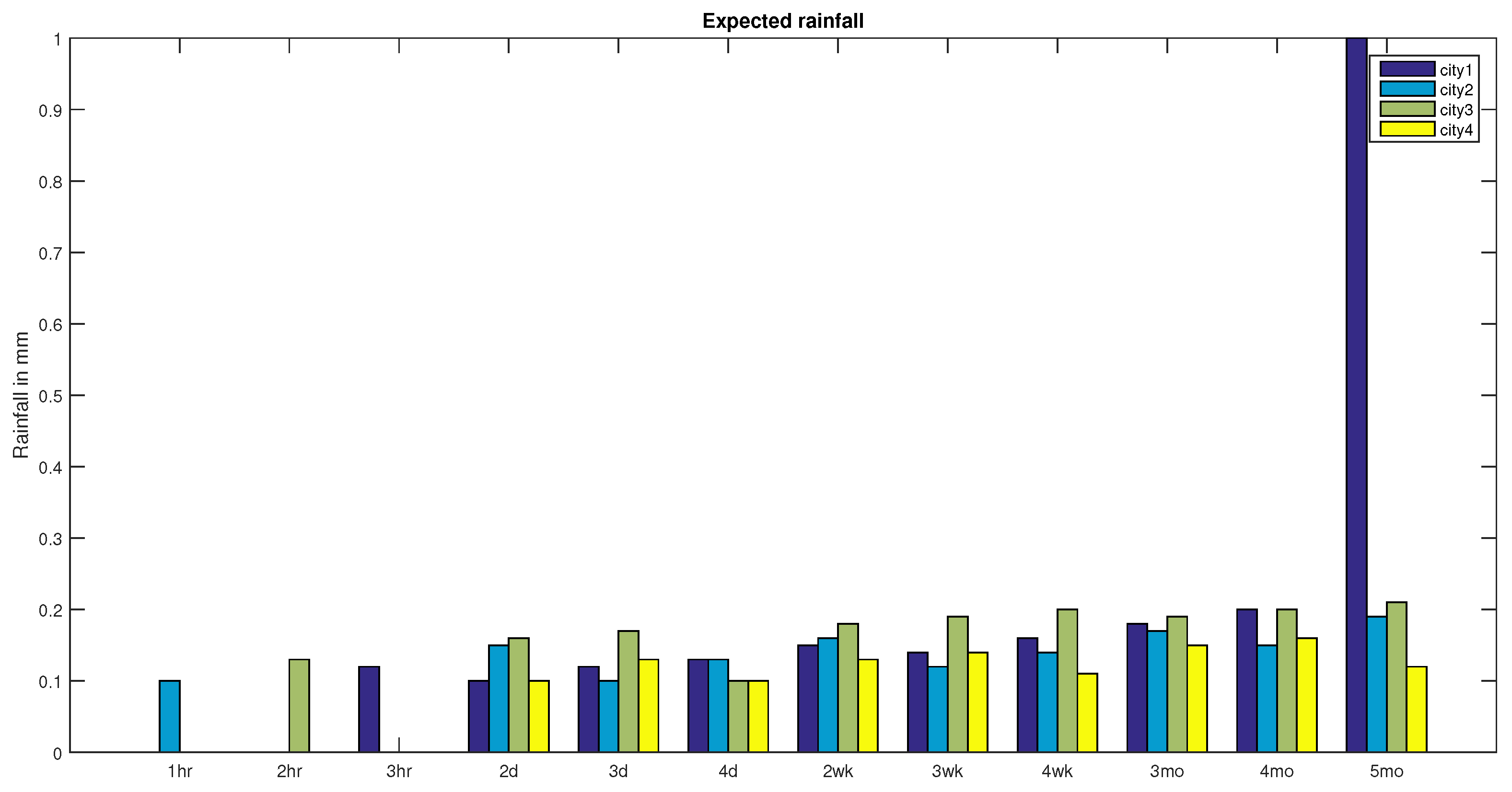
In this section, an application for the decision making by using the similarity measure of two $\mathcal{L}\mathcal{M}\mathcal{F}\mathcal{S}\mathcal{S}s$ to analyse the rainfall in 2016 and 2017 with expected rainfall.

Let $U_0=\{x_1,x_2,x_3,x_4\}$ be the universal set, where $x_1,x_2,x_3,x_4$ stands for the set of four cities in India. Let ${\mathsf{\Gamma }}_0=\{{\gamma }_1,{\gamma }_2,{\gamma }_3,{\gamma }_4\}$ as the parameters which is consider as the set of rainfalls in rainy season, where ${\gamma }_1$ stands for “Hour-wise rainfall” which includes 1 h, 2 h, and 3 h, ${\gamma }_2$ stands for “Day-wise rainfall” which includes 2 day, 3 day and 4 day, ${\gamma }_3$ stands for “Week-wise rainfall” which includes 2 week, 3 week, 4 week and ${\gamma }_4$ stands for “Month-wise rainfall” which includes 3 month, 4 month, 5 month respectively.

In this example, suppose $({\tilde{\mathcal{R}}}_0,{\mathsf{\Gamma }}_0)\in \mathcal{L}\mathcal{M}\mathcal{F}\mathcal{S}\mathcal{S}\left(U_0\right)$ represents the expected rainfall in India, defined as follows:

$({\tilde{\mathcal{R}}}_0,{\mathsf{\Gamma }}_0)=\{{\mathcal{R}}_0\left({\gamma }_1\right)=\{\frac{x_1}{(0,0,0.12)},\frac{x_2}{(0.1,0,0)},\frac{x_3}{(0,0.13,0)},\frac{x_4}{(0,0,0)}\}$,

${\mathcal{R}}_0\left({\gamma }_2\right)=\{\frac{x_1}{(0.1,0.12,0.13)},\frac{x_2}{(0.15,0.1,0.13)},\frac{x_3}{(0.16,0.17,0.1)},\frac{x_4}{(0.1,0.13,0.1)}\}$,

${\mathcal{R}}_0\left({\gamma }_3\right)=\{\frac{x_1}{(0.15,0.14,0.16)},\frac{x_2}{(0.16,0.12,0.14)},\frac{x_3}{(0.18,0.19,0.2)},\frac{x_4}{(0.13,0.14,0.11)}\}$

${\mathcal{R}}_0\left({\gamma }_4\right)=\{\frac{x_1}{(0.18,0.2,1)},\frac{x_2}{(0.17,0.15,0.19)},\frac{x_3}{(0.19,0.2,0.21)},\frac{x_4}{(0.15,0.16,0.12)}\}\}$.

Tabulation of $({\tilde{\mathcal{R}}}_0,{\mathsf{\Gamma }}_0)$ is given in

Table 5. Tabulation of $({\tilde{\mathcal{R}}}_0,{\mathsf{\Gamma }}_0)$ Representing the Expected Rainfall.

$({\tilde{\mathcal{R}}}_0,{\mathsf{\Gamma }}_0)$	${\mathit{x}}_1$	${\mathit{x}}_2$	${\mathit{x}}_3$	${\mathit{x}}_4$
${\gamma }_1$	(0,0,0.12)	(0.1,0,0)	(0,0.13,0)	(0,0,0)
${\gamma }_2$	(0.1,0.12,0.13)	(0.15,0.1,0.13)	(0.16,0.17,0.1)	(0.1,0.13,0.1)
${\gamma }_3$	(0.15,0.14,0.16)	(0.16,0.12,0.14)	(0.18,0.19,0.2)	(0.13,0.14,0.11)
${\gamma }_4$	(0.18,0.2,1)	(0.17,0.15,0.19)	(0.19,0.2,0.21)	(0.15,0.16,0.12)

and Figure 1.

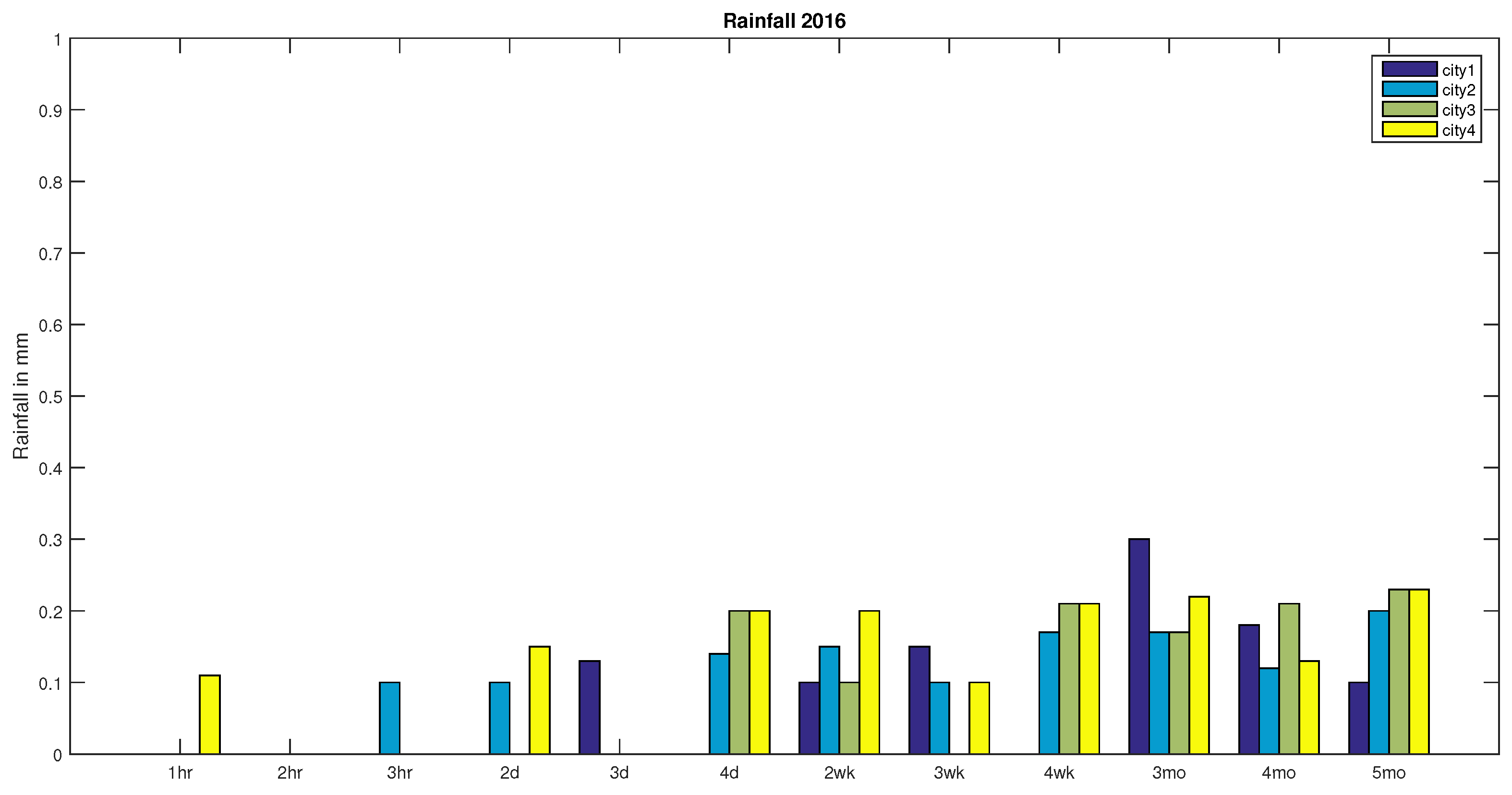
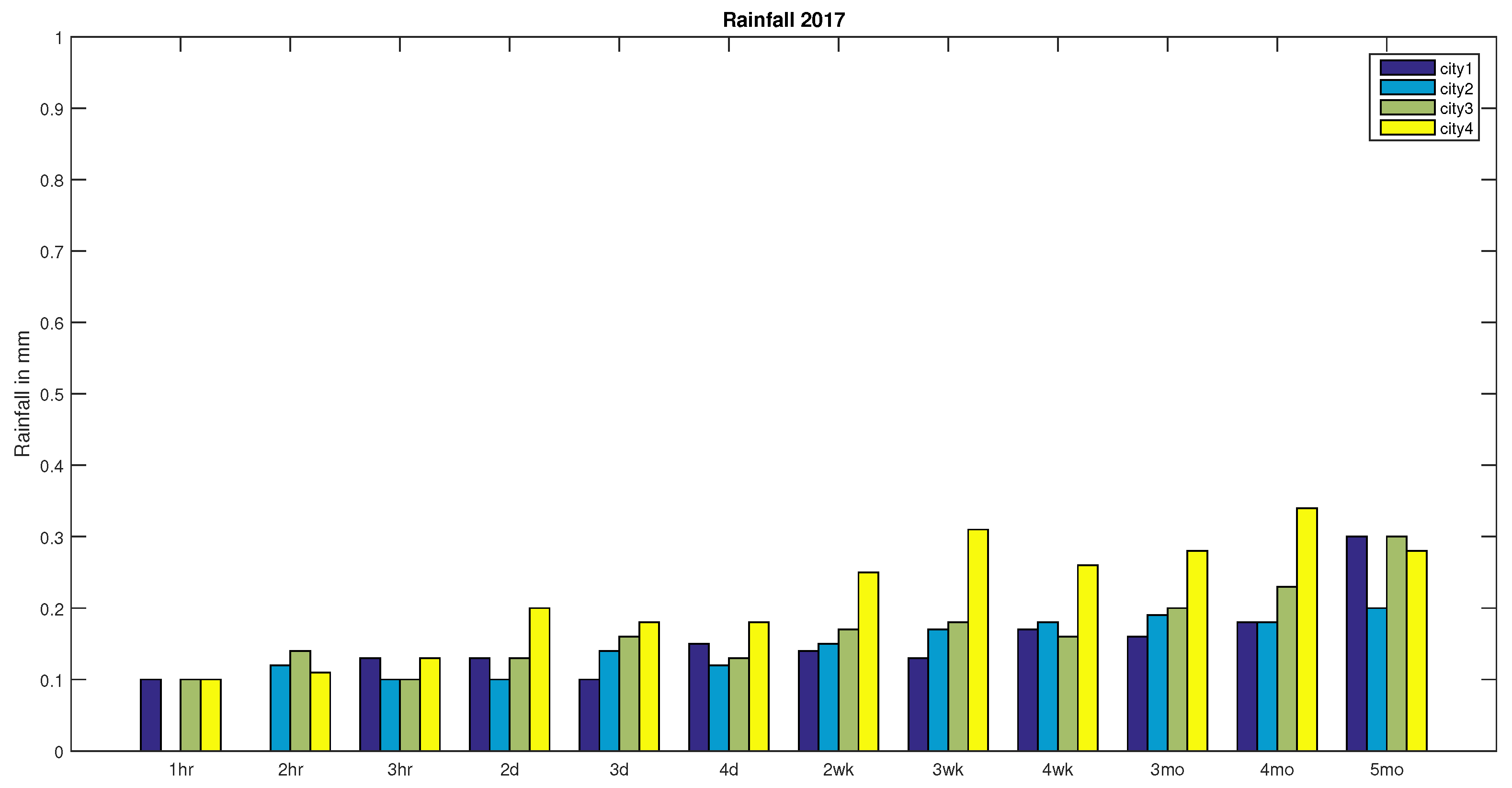
Now let $({\tilde{\mathcal{H}}}_1,{\mathsf{\Gamma }}_0),({\tilde{\mathcal{H}}}_2,{\mathsf{\Gamma }}_0)\in \mathcal{L}\mathcal{M}\mathcal{F}\mathcal{S}\mathcal{S}\left(U_0\right)$ represents the recorded rainfall in India for the year 2016 and 2017 respectively, defined as follows:

$({\tilde{\mathcal{H}}}_1,{\mathsf{\Gamma }}_0)=\{{\mathcal{H}}_1\left({\gamma }_1\right)=\{\frac{x_1}{(0,0,0)},\frac{x_2}{(0,0,0.1)},\frac{x_3}{(0,0,0)},\frac{x_4}{(0.11,0,0)}\}$,

${\mathcal{H}}_1\left({\gamma }_2\right)=\{\frac{x_1}{(0,0.13,0)},\frac{x_2}{(0.1,0,0.14)},\frac{x_3}{(0,0,0.2)},\frac{x_4}{(0.15,0,0.2)}\}$,

${\mathcal{H}}_1\left({\gamma }_3\right)=\{\frac{x_1}{(0.1,0.15,0)},\frac{x_2}{(0.15,0.1,0.17)},\frac{x_3}{(0.1,0,0.21)},\frac{x_4}{(0.2,0.1,0.21)}\}$

${\mathcal{H}}_1\left({\gamma }_4\right)=\{\frac{x_1}{(0.3,0.18,0.1)},\frac{x_2}{(0.17,0.12,0.2)},\frac{x_3}{(0.17,0.21,0.23},\frac{x_4}{(0.22,0.13,0.23)}\}\}$,

$({\tilde{\mathcal{H}}}_2,{\mathsf{\Gamma }}_0)=\{{\mathcal{H}}_2\left({\gamma }_1\right)=\{\frac{x_1}{(0.1,0,0.13)},\frac{x_2}{(0,0.12,0.1)},\frac{x_3}{(0.1,0.14,0.1)},\frac{x_4}{(0.1,0.11,0.13)}\}$,

${\mathcal{H}}_2\left({\gamma }_2\right)=\{\frac{x_1}{(0.13,0.1,0.15)},\frac{x_2}{(0.1,0.14,0.12)},\frac{x_3}{(0.13,0.16,0.13)},\frac{x_4}{(0.2,0.18,0.18)}\}$,

${\mathcal{H}}_2\left({\gamma }_3\right)=\{\frac{x_1}{(0.14,0.13,0.17)},\frac{x_2}{(0.15,0.17,0.18)},\frac{x_3}{(0.17,0.18,0.16)},\frac{x_4}{(0.25,0.31,0.26)}\}$

${\mathcal{H}}_2\left({\gamma }_4\right)=\{\frac{x_1}{(0.16,0.18,0.3)},\frac{x_2}{(0.19,0.18,0.2)},\frac{x_3}{(0.2,0.23,0.3)},\frac{x_4}{(0.28,0.34,0.28)}\}\}$.

Tabulations of $({\tilde{\mathcal{H}}}_1,{\mathsf{\Gamma }}_0)$ and $({\tilde{\mathcal{H}}}_2,{\mathsf{\Gamma }}_0)$ are presented as in

Table 6. Tabulation of $({\tilde{\mathcal{H}}}_1,{\mathsf{\Gamma }}_0)$ Representing the Rainfall 2016.

$({\tilde{\mathcal{H}}}_1,{\mathsf{\Gamma }}_0)$	${\mathit{x}}_1$	${\mathit{x}}_2$	${\mathit{x}}_3$	${\mathit{x}}_4$
${\gamma }_1$	(0,0,0)	(0,0,0.1)	(0,0,0)	(0.11,0,0)
${\gamma }_2$	(0,0.13,0)	(0.1,0,0.14)	(0,0,0.2)	(0.15,0,0.2)
${\gamma }_3$	(0.1,0.15,0)	(0.15,0.1,0.17)	(0.1,0,0.21)	(0.2,0.1,0.21)
${\gamma }_4$	(0.3,0.18,0.1)	(0.17,0.12,0.2)	(0.17,0.21,0.23)	(0.22,0.13,0.23)

and

Table 7. Tabulation of $({\tilde{\mathcal{H}}}_2,{\mathsf{\Gamma }}_0)$ Representing the Rainfall in 2017.

$({\tilde{\mathcal{H}}}_2,{\mathsf{\Gamma }}_0)$	${\mathit{x}}_1$	${\mathit{x}}_2$	${\mathit{x}}_3$	${\mathit{x}}_4$
${\gamma }_1$	(0.1,0,0.13)	(0,0.12,0.1)	(0.1,0.14,0.1)	(0.1,0.11,0.13)
${\gamma }_2$	(0.13,0.1,0.15)	(0.1,0.14,0.12)	(0.13,0.16,0.13)	(0.2,0.18,0.18)
${\gamma }_3$	(0.14,0.13,0.17)	(0.15,0.17,0.18)	(0.17,0.18,0.16)	(0.25,0.31,0.26)
${\gamma }_4$	(0.16,0.18,0.3)	(0.19,0.18,0.2)	(0.2,0.23,0.3)	(0.28,0.34,0.28)

and Figure 2 and Figure 3 respectively.

In order to make the decision of whether the rainfall in 2016 or the rainfall in 2017 is the expected rainfall in India, we use similarity measure on $\mathcal{L}\mathcal{M}\mathcal{F}\mathcal{S}\mathcal{S}s$ to calculate the similarity between the expected rainfall and the rainfall in 2016 ($\mathbf{S}(({\tilde{\mathcal{R}}}_0,{\mathsf{\Gamma }}_0),({\tilde{\mathcal{H}}}_1,{\mathsf{\Gamma }}_0))$); the similarity between the expected rainfall and the rainfall in 2017 ($\mathbf{S}(({\tilde{\mathcal{R}}}_0,{\mathsf{\Gamma }}_0),({\tilde{\mathcal{H}}}_2,{\mathsf{\Gamma }}_0))$). Comparing the obtained results, the higher similarity means the closer to expected rainfall.

First we calculate the similarity measure between $({\tilde{\mathcal{R}}}_0,{\mathsf{\Gamma }}_0)$ and $({\tilde{\mathcal{H}}}_1,{\mathsf{\Gamma }}_0)$:

$$\begin{array}{cc}& S_1(({\tilde{\mathcal{R}}}_0,{\mathsf{\Gamma }}_0),({\tilde{\mathcal{H}}}_1,{\mathsf{\Gamma }}_0))\hfill \\ =& \frac{(0\vee 0\vee 0\vee 0)+(0\vee 0.1\vee 0\vee 0.1)+(0.1\vee 0.15\vee 0.1\vee 0.13)+(0.18\vee 0.17\vee 0.17\vee 0.15)}{0\vee 0.1\vee 0\vee 0.11+0.1\vee 0.15\vee 0.16\vee 0.15+0.15\vee 0.16\vee 0.18\vee 0.2+0.3\vee 0.17\vee 0.19\vee 0.22}\hfill \\ =& \frac{0+0.1+0.15+0.18}{0.1+0.18+0.2+0.18}=0.39\hfill \end{array}$$

$$\begin{array}{cc}& S_2(({\tilde{\mathcal{R}}}_0,{\mathsf{\Gamma }}_0),({\tilde{\mathcal{H}}}_1,{\mathsf{\Gamma }}_0))\hfill \\ =& \frac{(0\vee 0\vee 0\vee 0)+(0.12\vee 0\vee 0\vee 0)+(0.14\vee 0.1\vee 0\vee 0.1)+(0.18\vee 0.12\vee 0.2\vee 0.13)}{0\vee 0\vee 0\vee 0+0.13\vee 0.1\vee 0.17\vee 0.13+0.15\vee 0.12\vee 0.19\vee 0.14+0.2\vee 1\vee 0.21\vee 0.16}\hfill \\ =& \frac{0+0.12+0.14+0.2}{0+0.17+0.19+1}=0.33\hfill \end{array}$$

$$\begin{array}{cc}& S_3(({\tilde{\mathcal{R}}}_0,{\mathsf{\Gamma }}_0),({\tilde{\mathcal{H}}}_1,{\mathsf{\Gamma }}_0))\hfill \\ =& \frac{(0\vee 0\vee 0\vee 0)+(0\vee 0.13\vee 0.1\vee 0.1)+(0\vee 0.14\vee 0.2\vee 0.11)+(0.1\vee 0.19\vee 0.21\vee 0.12)}{0.12\vee 0.1\vee 0\vee 0+0.13\vee 0.14\vee 0.2\vee 0.2+0.16\vee 0.17\vee 0.21\vee 0.21+1\vee 0.2\vee 0.23\vee 0.23}\hfill \\ =& \frac{0+0.13+0.2+0.21}{0.12+0.2+0.21+1.0}=0.35\hfill \end{array}$$

Hence $\mathbf{S}(({\tilde{\mathcal{R}}}_0,{\mathsf{\Gamma }}_0),({\tilde{\mathcal{H}}}_1,{\mathsf{\Gamma }}_0))=\frac{0.39+0.33+0.35}{3}=0.36$.

Next we calculate the similarity measure between $({\tilde{\mathcal{R}}}_0,{\mathsf{\Gamma }}_0)$ and $({\tilde{\mathcal{H}}}_2,{\mathsf{\Gamma }}_0)$:

$$\begin{array}{cc}& S_1(({\tilde{\mathcal{R}}}_0,{\mathsf{\Gamma }}_0),({\tilde{\mathcal{H}}}_2,{\mathsf{\Gamma }}_0))\hfill \\ =& \frac{(0\vee 0\vee 0\vee 0)+(0.1\vee 0.1\vee 0.13\vee 0.1)+(0.14\vee 0.15\vee 0.17\vee 0.13)+(0.16\vee 0.17\vee 0.19\vee 0.15)}{0.1\vee 0.1\vee 0.1\vee 0.11+0.13\vee 0.15\vee 0.16\vee 0.2+0.15\vee 0.16\vee 0.18\vee 0.25+0.18\vee 0.19\vee 0.2\vee 0.28}\hfill \\ =& \frac{0+0.13+0.17+0.19}{0.1+0.2+0.25+0.28}=0.59\hfill \end{array}$$

$$\begin{array}{cc}& S_2(({\tilde{\mathcal{R}}}_0,{\mathsf{\Gamma }}_0),({\tilde{\mathcal{H}}}_2,{\mathsf{\Gamma }}_0))\hfill \\ =& \frac{(0\vee 0\vee 0.13\vee 0)+(0.1\vee 0.1\vee 0.16\vee 0.13)+(0.13\vee 0.12\vee 0.18\vee 0.14)+(0.18\vee 0.15\vee 0.2\vee 0.16)}{0\vee 0.12\vee 0.14\vee 0.11+0.12\vee 0.14\vee 0.17\vee 0.18+0.14\vee 0.17\vee 0.19\vee 0.31+0.2\vee 0.18\vee 0.23\vee 0.34}\hfill \\ =& \frac{0.13+0.16+0.18+0.2}{0.14+0.18+0.31+0.34}=0.691\hfill \end{array}$$

$$\begin{array}{cc}& S_3(({\tilde{\mathcal{R}}}_0,{\mathsf{\Gamma }}_0),({\tilde{\mathcal{H}}}_2,{\mathsf{\Gamma }}_0))\hfill \\ =& \frac{(0.12\vee 0\vee 0\vee 0)+(0.13\vee 0.12\vee 0.1\vee 0.1)+(0.16\vee 0.14\vee 0.16\vee 0.11)+(0.3\vee 0.19\vee 0.21\vee 0.12)}{0.13\vee 0.1\vee 0.1\vee 0.13+0.15\vee 0.13\vee 0.13\vee 0.18+0.17\vee 0.18\vee 0.2\vee 0.26+1.0\vee 0.2\vee 0.3\vee 0.28}\hfill \\ =& \frac{0.12+0.13+0.16+0.21}{0.13+0.18+0.26+1.0}=0.395\hfill \end{array}$$

Hence $\mathbf{S}(({\tilde{\mathcal{R}}}_0,{\mathsf{\Gamma }}_0),({\tilde{\mathcal{H}}}_2,{\mathsf{\Gamma }}_0))=\frac{0.59+0.691+0.395}{3}=0.559$.

It is clear from the above results, that $({\tilde{\mathcal{H}}}_2,{\mathsf{\Gamma }}_0)$ has significantly greater similarity to $({\tilde{\mathcal{R}}}_0,{\mathsf{\Gamma }}_0)$, as compared with $({\tilde{\mathcal{H}}}_1,{\mathsf{\Gamma }}_0)$ to $({\tilde{\mathcal{R}}}_0,{\mathsf{\Gamma }}_0)$. So we conclude that the rainfall in 2016 is not an expected rainfall and the rainfall in 2017 is an expected rainfall in India.

5. Discussion

In this paper, our motivation to introduce the concept of similarity between two $\mathcal{L}\mathcal{M}\mathcal{F}\mathcal{S}\mathcal{S}$ is achieved. This similarity measure satisfies the good properties of similarity measures. Advantages of similarity measure on lattice ordered multi-fuzzy soft set include:

-

It is simple and very efficient to evaluate.

-

Many authors defined the fuzzy similarity measure in one dimension but some problems are difficult to explain in one dimension. To avoid the difficulties, we introduce the similarity measure in multi-dimension using the lattice structure.

The disadvantage of the proposed similarity measure is that it is only applicable to lattice ordered structures and does not work for other fuzzy structures.

Some properties of proposed measure are stated and proved by a theorem. Apart from that, an application for the decision making by using the similarity measure of two $\mathcal{L}\mathcal{M}\mathcal{F}\mathcal{S}\mathcal{S}$ to analyse the rainfall is obtained in this research. This application shows that our proposed measure is worth to use.

6. Conclusions

Multi-fuzzy soft set and its extensions are used in many different applications in decision making. The similarity measure on complex multi-fuzzy soft set has been proposed. $\mathcal{L}\mathcal{M}\mathcal{F}\mathcal{S}\mathcal{S}$ was applied in solving forecast problems, but the similarity on $\mathcal{L}\mathcal{M}\mathcal{F}\mathcal{S}\mathcal{S}$ was not introduced. In this paper, the concept of similarity measure of $\mathcal{L}\mathcal{M}\mathcal{F}\mathcal{S}\mathcal{S}$ is introduced. The numerical examples are presented in detail to illustrate the proposed similarity measure. We also define some properties of similarity measure on two $\mathcal{L}\mathcal{M}\mathcal{F}\mathcal{S}\mathcal{S}s$. These properties are proved by Theorem 3.3. Finally, an application of this similarity measure in decision making is presented.

In further works, we are going to extend the operations and properties of $\mathcal{L}\mathcal{M}\mathcal{F}\mathcal{S}\mathcal{S}$ using similarity measure. Besides, the using of this similarity measure in solving other real life problems will be studied.