An Evolutionary Algorithm-Based PWM Strategy for a Hybrid Power Converter

Abstract

In the past years, the interest in direct current to direct current converters has increased because of their application in renewable energy systems. Consequently, the research community is working on improving its efficiency in providing the required voltage to electronic devices with the lowest input current ripple. Recently, a hybrid converter which combines the boost and the Cuk converter in an interleaved manner has been introduced. The converter has the advantage of providing a relatively low input current ripple by a former strategy. However, it has been proposed to operate with dependent duty cycles, limiting its capacity to further decrease the input current ripple. Independent duty cycles can significantly reduce the input current ripple if the same voltage gain is achieved by an appropriate duty cycle combination. Nevertheless, finding the optimal duty cycle combination is not an easy task. Therefore, this article proposes a new pulse-width-modulation strategy for the hybrid interleaved boost-Cuk converter. The strategy includes the development of a novel mathematical model to describe the relationship between independent duty cycles and the input current ripple. The model is introduced to minimize the input current ripple by finding the optimal duty cycle combination using the differential evolution algorithm. It is shown that the proposed method further reduces the input current ripple for an operating range. Compared to the former strategy, the proposed method provides a more balanced power-sharing among converters.

1. Introduction

The electric and electronic devices usually require several voltage levels for their different components, dc-dc converters are electronic circuits that provide the required voltage to a certain component [1], such as a microprocessor in a computer, which requires a 1 V power supply and it is usually accompanied to a (direct current to direct current) dc-dc converter, to provide the required voltage level and power, the power converter for a microprocessor is usually dedicated since other digital circuits require different voltage levels, for example, 3.3 V or 5 V.

We can define a dc-dc converter as a power-electronics-based circuit that can change (and regulate) the voltage level from input to output, in a wide variety of applications and levels, for example, from 3.3 V to 1 V for microprocessors, or from but also from 12 V to 200 V, for photovoltaic panels applications.

The interest for dc-dc converters has recently grown because of their application in other fields such as renewable energy generation systems, especially with photovoltaic panels and fuel cells, those energy sources, have a relatively low output voltage, in the range of 10 to 40 volts, while grid-tie inverters require a voltage in the range of 200 V. Commercial solutions contain both the dc-dc converter and the inverter in a single package. The research community is working to improve both the dc-dc converter and the dc-ac inverter.

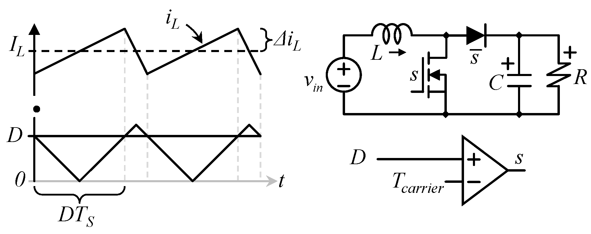
Dc-dc converters have a wide variety of topologies and applications, in the photovoltaic panels application, a step-up or boost topology is required (a converter that increases the voltage); Figure 1 shows the schematic of the traditional boost converter [1]. Those power electronics converters are controlled by Pulse Width Modulation (PWM), a technique in which transistors are open and closed periodically, and their operation is controlled by manipulating the width of pulses, or the time they remain closed. The main characteristics of its operation can be summarized as the switching functions of the transistor, or PWM is obtained by comparing a triangular carrier against a dc signal D, which represents the duty cycle, when D overpasses the triangular carrier, the transistor s is closed (on), the diode is called s to indicate it complementary to s, the transistor keeps closed a time DT_S, where T_S is the switching period, the inverse of the switching frequency f_S. In Figure 1, if the constant signal D decreases, their comparison with the triangular carrier will produce the time DT_S to get shorter, the relation between D divided over the peak value of the triangular carrier is the same as DT_S divided over T_S, making this comparison procedure, a simple manner to modify (modulate) the width of the pulses that control the open and close function of the transistor.

The inductor current i_L waveform is composed of their dc component I_L plus an ac (triangular) waveform; the maximum deviation from the dc component is called current ripple Δi_L.

The ripple can be calculated starting from the traditional inductor Equation (1) (see Equation (2.1) in [1]), which indicated the derivative of the current with respect to time in an inductor is equal to the voltage applied across their terminals.

$$L\frac{d{i}_L}{dt}=v_L$$

(1)

Equation (1) can be used to calculate the input current ripple, which in this converter, in which the inductor is connected in series with the input source, the input current ripple is equal to the inductor current ripple. If the inductor is connected to a constant voltage, the derivative equation becomes an incremental equation:

$$L\frac{\mathsf{\Delta }{i}_L}{\mathsf{\Delta }t}=V_L$$

(2)

This incremental Equation (2) is the reason why the derivatives or slopes in the signal i_L in Figure 1 are constant (it was two slopes, one positive and one negative, but they both seems as constant derivatives), when the switch is closed (which occurs during a time DT_S), the inductor is connected directly to the input voltage, as it can be seen in Figure 1, the current ripple is measured as half of the total current change. The current ripple (which is half of the total peak-to-peak variation), can be expressed as Equation (3), which is equivalent to Equation (2.43) in [1], note that Equation (3) utilizes the inverse of the switching period T_S, which is the switching frequency f_S.

$$\mathsf{\Delta }{i}_L=\frac{1}{2}\cdot \frac{V_{in}}{L}D{T}_S=\frac{V_{in}D}{2L{f}_S}$$

(3)

In the traditional boost converter (Figure 1), there are two practical ways (from the engineering point of view) of reducing the switching ripple, by increasing the inductance (L), or the switching frequency (f_S). As mentioned before, it is important to maintain a low input current ripple since this reduces the RMS current provided by the power source.

Another desirable characteristic of the dc-dc converter is to have a non-pulsating input current with low ripple. A pulsating current or current with large ripple produces an early aging of the renewable energy source [2], since their rms (the root mean square) value of the current is larger, which produces additional power conduction. The ideal situation would be having a constant input current with zero ripple, or a very small (negligible) ripple, but this may be impossible or too expensive in a real situation, for the full operating range of the converter.

The state-of-the-art of power electronics contains many topologies of dc-dc converters [3,4], among the different solutions, interleaved converters, such as the interleaved boost converter, have been successfully applied, several converters in parallel, each of them have a specific input-current switching-ripple, by shifting the switching functions of converters, the switching ripple or variation can get a kind of signal cancelation, while their dc components add together to have a more powerful converter with less input current ripple.

One of the operation rules in interleaved converters is that all parallel converters must have the same duty cycle, or voltage gain, since their input voltage is the same, if one of them try to increase the voltage more than another parallel converter, a severe power imbalance will destroy the system. A characteristic of interleaved converters is that they have operation points in which the input current ripple is zero, for example, the two-phases interleaved boost converter has zero input current ripple when the duty cycle is 0.5, this operation point depends on the number of interleaved phases and cannot be selected.

On the other hand, hybrid interleaved converters have been proposed, such as in [5]; for this particular converter, the zero-input current ripple can be selected; this allows us to operate the converter in their optimal operation region.

In the traditional interleaving converters, all converters have the same duty cycle; in the hybrid converter [5], the PWM strategy assigns one duty cycle depending on the other one, they are dependent. The hybrid converter may have independent duty cycles, but then, the same voltage gain can be achieved with infinite combinations of duty cycles, each combination with different input current ripple.

Finding the optimal combination of duty cycles is not an easy task. Therefore, this article proposes a new PWM strategy for the hybrid interleaved boost-Cuk converter [5]. The strategy includes the development of a novel mathematical optimization model to describe the relationship between independent duty cycles and the input current ripple. The model is introduced to minimize the input current ripple by finding the optimal duty cycles using the differential evolution (DE) algorithm.

It is shown that the proposed method further reduces the input current ripple for an operation range, compared against the former strategy, which already had a low input current ripple, the proposed strategy also provides a better (more balanced) power-sharing among converters.

2. Literature Review

In the past years, researchers have applied metaheuristic algorithms to solve complex optimization problems successfully. Some examples of powerful metaheuristic algorithms are differential evolution (DE) [6], genetic algorithm (GA) [7], and particle Swarm optimization (PSO) [8], to mention a few. These methods are considered some of the most popular techniques because they are accurate, simple, and easy to implement.

Recently, further sophisticated metaheuristic algorithms have been included in the literature, namely the Yellow Saddle Goatfish Algorithm (YSGA) [9], the distance-based parameter adaptation for Success-History based Differential Evolution (DbL-SHADE) [10], the Combined Evolutionary Game Particle Swarm Optimization (C-EGPSO) [11], and others [12,13,14,15,16,17]. These methods have proved their efficiency in a wide range of applications, including high-dimensional problems. However, the presented approaches are considered vastly complex and computationally expensive.

State-of-the-art metaheuristic techniques have been effectively applied to solve related optimization problems such as the improved interleaved boost converter [18], which uses the PSO algorithm to find the optimal Type-III controller. In [9], a chaotic version of the PSO algorithm is proposed to improve the maximum power point tracking capability for a photovoltaic system [19]. The PSO was also implemented for tuning gains in a PI controller of a four-phase interleaved boost converter [20]. On the other hand, the DE was used in [21] for the optimal design of high-power mode converters. Other related implementations of DE and PSO algorithm can be found in [22,23,24,25].

Although the presented approaches are somehow related to converters, the proposed strategy is different in all aspects, namely the type of converter and its topology, the specific energy system application, and the objective to be improved by the implemented optimization algorithm.

3. Converters of Interest

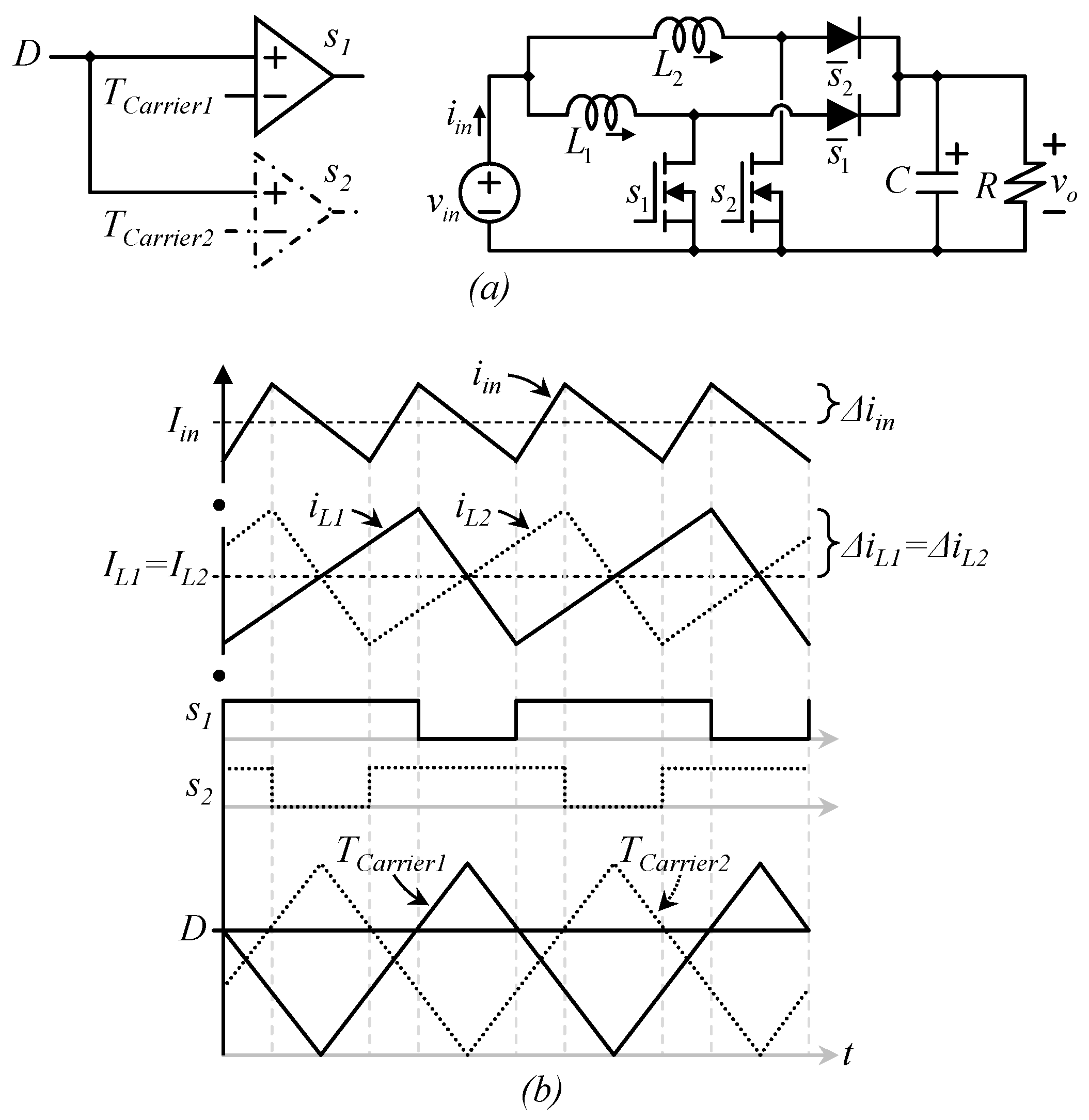
As mentioned before, interleaved converters are converters of the same type, connected in parallel, Figure 2a shows a two-phase interleaved boost converter (the number of converters is sometimes referred to as the number of phases), along with their PWM strategy, Figure 2b shows PWM waveforms at the bottom and important current waveforms, both switching functions have the same duty cycle, but triangular carriers are shifted 180°, which produces that switching functions are also shifted.

The input current is equal to the sum of the current through inductors, inductors drain the same dc current since duty cycles are equal, but the phase shift produces that their ac component (switching ripple), have a certain cancelation, and the input current ripple is smaller than the ripple in individual inductors.

The advantage is that smaller inductors can be selected to perform with the same current ripple of the single boost converter (Figure 1), despite the number of components, which is larger in Figure 2a, since passive components (inductors and capacitors) are smaller for the interleaved version, and electronic devices are getting miniaturized with the new technology, interleaved converters are usually smaller than their non-interleaved counterpart. The reduction of the size of inductors is especially beneficial since it is usually the largest and heaviest component in the circuit. The converters that accompany the computer microprocessor is an interleaved buck converter.

The interleaved boost converter actually achieves zero input current ripple, when the duty cycle is 0.5, switching functions are perfectly complementary in this case, but converters operate into a region of duty cycles, not a single one because they contain the closed-loop control which compensates the duty cycle if a perturbation occurs (such as a variation on the input voltage).

3.1. The Hybrid Converter with the Existing PWM Strategy

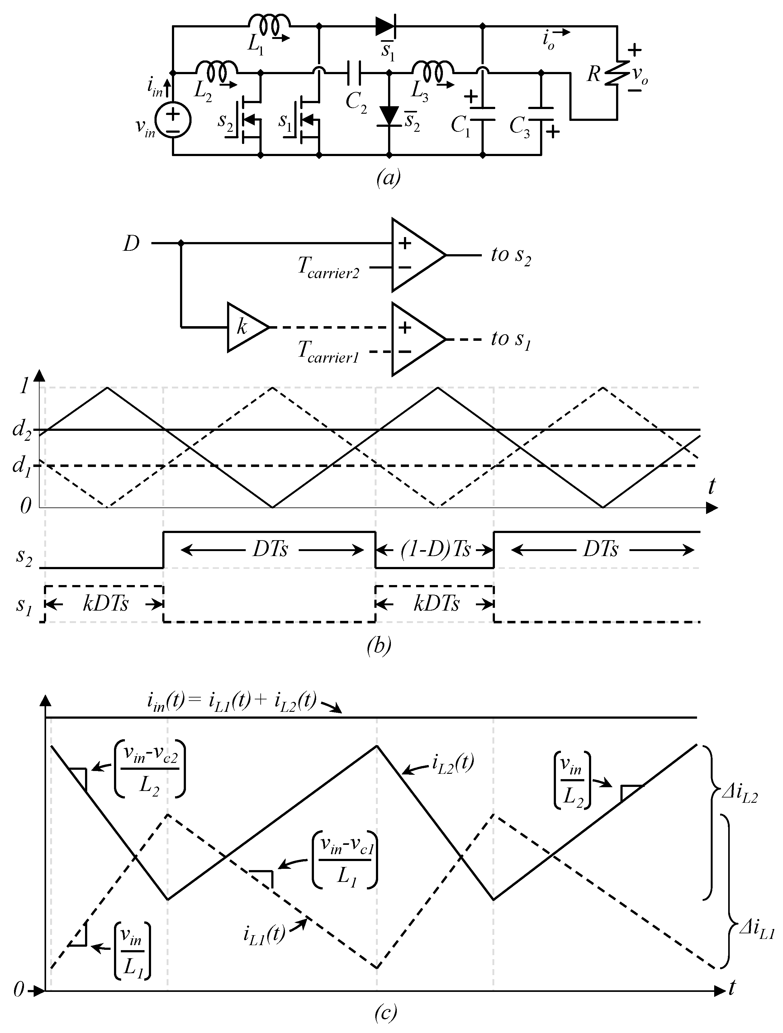
The hybrid converter under study is shown in Figure 3a, as proposed in [5], is made by the interconnection of a Cuk and a boost converter, they share the same input voltage, the load is connected in a differential mode from the output of the Cuk, to the output of the boost converter, since the Cuk provides a negative output voltage with respect to the boost converter, the voltage gain is larger than interleaving two boost converters since their outputs are independent, converters may have different duty cycles.

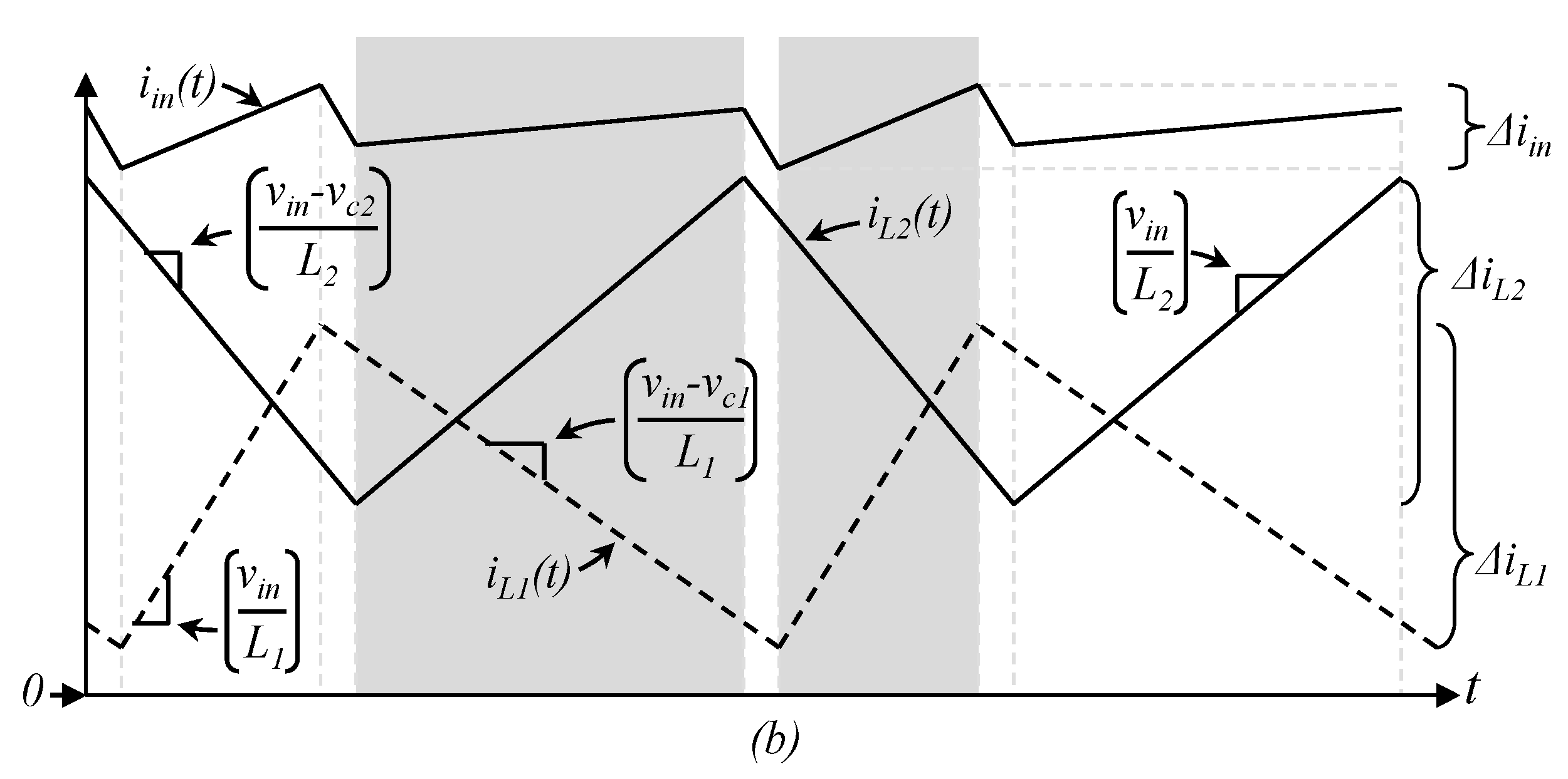
The capacity to operate with different duty cycles in each power stage is an additional degree of freedom, that was used in [5] to select the duty cycle in which the input current ripple is equal to zero. Figure 3c shows the PWM strategy, and Figure 3b shows current waveforms in the duty cycle in which the input current ripple is zero, the current through inductors have an ac component which perfectly cancels each other at the input side.

As mentioned before, this particular operation point is just one of an operation range. When the duty cycle changes (due to the operation of the closed-loop control), a ripple appears, similar to Figure 2, the ripple is still smaller compared to the current ripple in one inductor.

Having the freedom to choose the duty cycle in which the current ripple is zero, is an advantage, for example, let us think on an application of the traditional interleaved boost converter, in which zero ripple duty cycle is 0.5, if the operation range of the duty cycle is between 0.6 and 0.7, the converter will never reach their ideal operation, in that case, it would be beneficial to choose the ideal operation to be in the duty cycle of 0.65.

This article proposes to operate this converter with a novel PWM strategy, in which the converter still have the zero ripple duty cycle in a chosen value, but it will be shown that the proposed strategy reduces the input current ripple in the full operation range, in the vicinity of the zero ripple duty cycle. Furthermore, it will be shown that the proposed strategy also provides a better balance on power-sharing among converters. For this purpose, the switching ripple will be analyzed first in their current operation.

3.2. Mathematical Model of the Hybrid Converter

In order to analyze the input current-ripple of the converter, which depends on variables such as the input voltage, the inductance of inductors and the equilibrium state-variables of the system, am equilibrium model of the state variables, (current through inductors and voltage across capacitors) is introduced in this section.

Since converters that compose the hybrid converter are well-known with proven operation [1], their model can be straight forward presented, considering the state variables as the current through inductors and the voltage across capacitors, the state equilibrium can be expressed as:

$$V_{C1}=V_{in}\frac{1}{1-D_1}; I_{L1}=I_o\frac{1}{1-D_1}$$

(4)

$$V_{C2}=V_{in}\frac{1}{1-D_2}; I_{L2}=I_o\frac{D_2}{1-D_2}$$

(5)

$$V_{C3}=V_{in}\frac{1}{1-D_2}; I_{L3}=I_o$$

(6)

where D_x (x = 1, 2) is the duty cycle for each transistor s_x, the voltage V_Cy (y = 1, 2, 3) as the voltage of each capacitor C_y, and the current i_Lz (z = 1, 2, 3) as the current of each inductor L_z, a capital letter in equations indicates the equilibrium value of each variable; I_o represents the output current.

The output voltage is provided by the series connection of C₁ and C₃, considering the load resistance R, then the output characteristics can be expressed as Equation (7).

$$V_o=V_{in}\frac{1}{1-D_1}+V_{in}\frac{D_2}{1-D_2}; I_o=\frac{V_o}{R}$$

(7)

3.3. Current PWM Strategy

The current PWM strategy for the hybrid converter is based on the definition that the duty cycle of the converter is assigned to s₂, d = d₂, and the duty cycle of s₁ (d₁), is defined as a fraction of d by multiplying d by a factor k.

$$d=d_2; d_1=kd$$

(8)

By assigning the same relationship to inductors.

$$L_1=k{L}_2$$

(9)

The factor k can be calculated from the duty cycle in which the input current ripple is desired to be zero, this duty cycle can be named D_Z, and the relationship can be expressed as:

$$k=\frac{1-D_Z}{D_Z}$$

(10)

This is a straightforward procedure; a full explanation and design procedure were provided in [5]. The input current ripple must be explained in two different conditions, where D > D_Z, and then D < D_Z.

4. Proposed PWM Strategy

The current PWM strategy has a good performance, but when defining one duty cycle is proportional to the second one during the full operation range, a degree of freedom is lost, in the proposed strategy, the factor k is variable, duty cycles can be still expressed as in Equation (8), but k is not constant, and we can choose the best value in each operation point.

The factor k, which now is variable, defines the relationship among duty cycles, inductors cannot be changed during the operation, their relationship is constant, and then, a second factor is defined k_L, which is constant and defines the relationship among inductors:

$$L_1=k_L{L}_2$$

(11)

Now there are two variables to choose during the operation, which are either duty cycles D₁ and D₂, or the general duty cycle D and the factor k. A challenge arises, there is an infinite number of combinations of those two variables to achieve certain voltage gain. In the former strategy, when k was constant, there was one duty cycle for each voltage gain. The strategy consists of choosing the combination of D and k, which minimizes the input current ripple.

It is intuitively expected that during the zero-ripple gain, k will be equal to k_L, but in other cases, it will be different, and this degree of freedom can be used to further reduce the input current ripple.

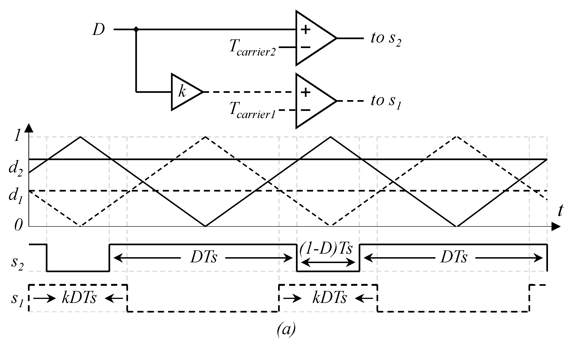
4.1. The Case When D > D_Z

Let us start with the case then D > D_Z, in other words, when there is an overlap on the switching functions, see Figure 4, under those conditions, there are two different periods in which the maximum ripple may appear (in gray in Figure 4): (1 − kD)T_S (the large gray period in Figure 4) and (1 − D)T_S (the short gray period in Figure 4).

During the period (1 − kD)T_S, the input current ripple may be expressed as Equation (12).

$${\mathsf{\Delta }}_{ig}=\left(1-kD\right)T_S\left(\frac{V_{in}}{L_2}+\frac{V_{in}-V_{C1}}{L_1}\right)$$

(12)

Which, considering Equations (4) and (8), can be simplified as Equation (13).

$${\mathsf{\Delta }}_{igA}=\frac{V_{in}{T}_S}{L_2{k}_L}\left(k_L-kD-k_{L}kD\right)$$

(13)

During the period (1 − D)T_S, the input current ripple may be expressed as Equation (14).

$${\mathsf{\Delta }}_{ig}=\left(1-kD\right)T_S\left(\frac{V_{in}}{L_1}+\frac{V_{in}-V_{C2}}{L_2}\right)$$

(14)

Which, considering Equations (5) and (8) can be simplified as:

$${\mathsf{\Delta }}_{igB}=\frac{V_{in}{T}_S}{L_2{k}_L}\left(1-D-k_{L}D\right)$$

(15)

Since there are two different periods in which the current ripple may reach a maximum value, the optimization algorithm must minimize them both; intuitively, they are expected to be equal to each other. Similarly, when D < D_Z, there are two periods in which the maximum current ripple may appear.

4.2. The Case When D < D_Z

When D < D_Z, there is a dead-time (a period in which transistors are both off) on the switching functions, see Figure 5, under those conditions, there are two different periods in which the maximum ripple may appear, marked in gray in Figure 5, those periods are DT_S (the large gray period in Figure 5) and kDT_S (the short gray period in Figure 5).

During the period DT_S, the input current ripple may be expressed as Equation (16).

$${\mathsf{\Delta }}_{ig}=D{T}_S\left(\frac{V_{in}}{L_2}+\frac{V_{in}-V_{C1}}{L_1}\right)$$

(16)

Which, considering Equations (4) and (8), can be simplified as Equation (17).

$${\mathsf{\Delta }}_{ig{A}_2}=\frac{V_{in}{T}_S}{L_2{k}_L}\frac{D}{\left(1-kD\right)}\left(k_L-kD-k_{L}kD\right)$$

(17)

During the period kDT_S, the input current ripple may be expressed as Equation (18).

$${\mathsf{\Delta }}_{ig}=kD{T}_S\left(\frac{V_{in}}{L_1}+\frac{V_{in}-V_{C2}}{L_2}\right)$$

(18)

Which, considering Equations (5) and (8) can be simplified as:

$${\mathsf{\Delta }}_{ig{B}_2}=\frac{V_{in}{T}_S}{L_2{k}_L}kD\left(1-D-k_{L}D\right)$$

(19)

Then, the algorithm to choose the duty cycle D, and the scalar factor k, must minimize Equations (13) and (14) in the case the gain requires a D > D_Z, and Equations (17) and (19) otherwise, this can be an iterative process, at the same time, the algorithm must comply the gain, which can be expressed from Equation (7) as Equation (20).

$$G=\frac{1}{1-kD}+\frac{D}{1-D}$$

(20)

5. The Optimization Process

Evolutionary-based metaheuristics and swarm intelligence algorithms, such as particle swarm optimization (PSO), firefly algorithm (FA), genetic algorithm (GA), cuckoo search (CS), grey wolf optimizer (GWO), and ant colony optimization (ACO) has been extensively used for solving complex optimization problems. Some recent applications on the industry are described in [26], where authors reported that the PSO had been mainly implemented in the electric power industry, including as the most popular areas the reactive power and voltage control, system identification, and intelligent control, and the generation expansion problem. Moreover, ACO has been primarily used for machine learning tasks such as feature selection and parameter optimization for support vector machines. According to the authors, other applications of the ACO include fields such as data mining, energy savings in wireless sensor networks, and water distribution systems.

On the other hand, in [27], an evolutionary-based algorithm has been used for truck scheduling at cross-docking terminals. It analyses the performances of the evolutionary method in finding the optimal schedule by varying the mutation levels. Also, a delayed start parallel evolutionary algorithm has been proposed for truck scheduling at a cross-docking facility [28].

The performance of swarm-based algorithms has also been analyzed in other real applications, such as for wind farm decision systems in [29], where the authors included optimization algorithms, namely FA, CS, GA, and ACO. Furthermore, a review of swarm-based algorithms for feature selection is presented in [30]. In the survey, the performances of the most promising swarm intelligence methods, namely PSO, ACO, FA, and GWO, are analyzed. Finally, a supervised learning approach based on PSO is introduced for social aware cognitive radio handovers in [31].

The presented real applications have proved the efficiency of evolutionary-based and swarm-based metaheuristics for solving complex optimization problems. Therefore, an evolutionary method, which can also be considered as a swarm-based technique, has been selected in this research.

In the proposed technique, the differential evolution (DE) algorithm is used to optimize the general duty cycle D and the factor k. The objective is to choose the best values of D and k in each operation point, such that their combination minimizes the input current ripple.

5.1. Differential Evolution Algorithm

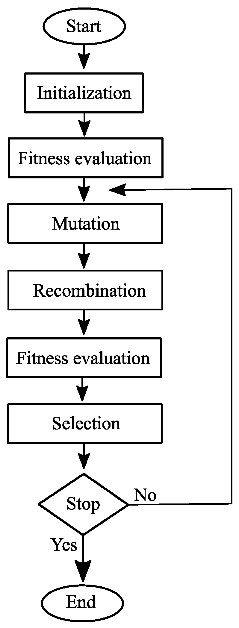
The differential evolution algorithm is a popular evolutionary algorithm (EA) that is based on operators such as mutation, recombination, and selection. In its basic operation, the DE algorithm uses a set of search agents X = {x₁, x₂ ..., x_m}, where each individual x_i represents a potential solution that improves over time under an evolutionary process.

The DE algorithm starts by randomly initializing the population, which is evaluated in the fitness function. After that, individuals evolve in an iterative process by the influence of mutation, recombination, and selection operators.

Under the mutation operator, individuals are transformed by a mutant vector, which is calculated as Equation (21):

$$v=x_{r_3}+F\left(x_{r_1}-x_{r_2}\right)$$

(21)

where the mutant vector is v and $F$ is a weighted factor whose values are in the interval of [0, 2], elements x_r1, x_r2, and x_r3, are randomly selected particles from the set of search agents.

In the recombination process, new candidate solutions are generated by combining the mutant vector v with an individual x_i. The result from this combination is a trial solution u, which is defined by Equation (22):

$$u_{ij}=\{\begin{array}{l}{v}_{ij},rand\left(0,1\right)\le p\\ x_{ij},otherwise\end{array}$$

(22)

where p is the recombination probability parameter, while rand represents a random value in the interval [0, 1], subscript j corresponds to the index of the problem dimension. After recombination, the population is evaluated in the fitness function.

The last operation of the DE algorithm is the selection of the best elements. The selection determines which individuals will remain for the next generation and which will be discarded. Considering the problem is a minimization type, the selection is based on the fitness value of candidate solutions u and x_i, which can be expressed as Equation (23).

$$x_i=\{\begin{array}{l}u,f\left(u\right)<f\left(x_i\right)\\ x_i,otherwise\end{array}$$

(23)

where f(u) and f(x_i) are the fitness values of u and x_i, respectively.

The process of mutation, recombination, and selection is repeated in an iterative process until a stop criterion is reached. The described DE algorithm can be summarized in Figure 6.

At the end of the search process, the solution is the best element among the population. The best individual is considered the global best particle whose fitness value is the lowest in the population.

5.2. Proposed Mathematical Model

In order to optimize the general duty cycle D and the factor k by implementing the DE algorithm, a mathematical model is proposed. This model acts as the objective function and is used to minimize the input current ripple.

Since there are two different periods in which the current ripple may reach a maximum value, the objective function must be designed to minimize the highest input current ripple. Considering the case when D > D_Z, the model contemplates the minimization of the highest input current ripple between definitions Equations (13) and (15). Similarly, when D < D_Z, the highest input current ripple among Equations (17) and (19) is minimized under the designed cost function.

Additionally, the proposed model must include some constraints such as the achievement of the desired voltage gain, the input current ripple considering the switching time, and the search domain that contemplates the permissible values of D and k. Under the above restrictions, the proposed model can be expressed as Equation (24):

$${\displaystyle \underset{D,k\in ℝ}{\min }}f\left(D,k\right)=\{\begin{array}{l}{f}_1\left(D,k\right),D>D_Z\\ f_2\left(D,k\right),otherwise\end{array}.$$

(24)

Subject to

$$G\le \frac{1}{1-kD}+\frac{D}{1-D}\le G+t.$$

(25)

$$0\le D\le 1.$$

(26)

$$0\le k\le 1.$$

(27)

where t is the permissible tolerance, which considers the 1% of the desired voltage gain G, while f₁(D,k) and f₂(D,k) are defined in Equations (28) and (29), respectively:

$$f_1\left(D,k\right)=\{\begin{array}{l}\left|{\mathsf{\Delta }}_{igA}\right|,\left|{\mathsf{\Delta }}_{igA}\right|>\left|{\mathsf{\Delta }}_{igB}\right|\\ \left|{\mathsf{\Delta }}_{igB}\right|,otherwise\end{array}.$$

(28)

$$f_2\left(D,k\right)=\{\begin{array}{l}\left|{\mathsf{\Delta }}_{ig{A}_2}\right|,\left|{\mathsf{\Delta }}_{ig{A}_2}\right|>\left|{\mathsf{\Delta }}_{ig{B}_2}\right|\\ \left|{\mathsf{\Delta }}_{ig{B}_2}\right|,otherwise\end{array}.$$

(29)

5.3. Implementation of DE in the Proposed Model

To minimize the highest input current ripple, the implementation of the DE algorithm must consider each individual from the population as a bidimensional vector that represents the combination of the possible values of D and k. Therefore, an individual x_i is defined as Equation (30).

$$x_i=\left\{D,k\right\}.$$

(30)

The quality of the candidate solution is given by the evaluation of x_i in the objective function described by Equation (24). Thus, Equation (24) can be rewritten as Equation (31):

$${\displaystyle \underset{x_i\in ℝ}{\min }}f(x_i)=\{\begin{array}{l}{f}_1\left(D,k\right),D>D_Z\\ f_2\left(D,k\right),otherwise\end{array}.$$

(31)

Since the proposed model represents a constrained optimization problem, the evaluation of the population in the objective function requires the implementation of a penalty function. This function is employed to modify the fitness value of a candidate solution when one or more constraints are not met. Thus, the penalty function is used to guide the search toward feasible solutions. In the proposed strategy, the penalty function is expressed as in Equation (32):

$$h=\left|wc\left(G-\frac{1}{1-x_{i1}{x}_{i2}}-\frac{x_{i1}}{1-x_{i1}}\right)\right|.$$

(32)

where w is a constant factor that regulates how much the fitness value of a candidate solution is penalized. The violated constrain indicator is c, where c ϵ {0, 1}. The value of c is 1 when the constraint described in Equation (25) is not fulfilled; this value will activate the penalty function. Otherwise, its value is 0, additionally, x_i1 = D and x_i2 = k.

Considering the penalty function for the evaluation of the population, the objective function defined in Equation (31) can be rewritten as Equation (33):

$${\displaystyle \underset{x_i\in ℝ}{\min }}f\left(x_i\right)+h.$$

(33)

In the optimization process, a population of m candidate solutions is randomly initialized under the lower and upper bounds defined by Equations (26) and (27). Then, the population is evaluated in the objective function given by Equation (33). After that, the iterative process begins, where individuals are mutated and recombined by using Equations (21) and (22), respectively. Finally, the best elements are selected to be the new population, which will be part of the next generation. The process is repeated until the maximum number of generations g_max is reached. The complete procedure is summarized in Algorithm 1.

Algorithm 1. Optimization process.

Input: m, gmax Output: D,k Parameter configuration: F, p, w Initialize the population Evaluate the population using Equation (33) Identify the global best individual For each element xi in the population | Generate the mutant vector v using Equation (21) | Generate the trial solution u using Equation (22) | Select the best individual using Equation (23) End for Update the global best individual If the number of generations gmax has not been reached | Go to step 5 Else | The solution is the global best individual End if-else End the search process

6. Experiments and Results

Several numerical experiments have been conducted to evaluate the performance of the proposed technique, where the former strategy is compared with the proposed method.

In the experiments, different desired voltage gain values are considered to demonstrate the robustness of our technique. These values range from 3 to 6, which are a representative sample of the most significant values.

Regarding the parameter configuration of the DE method, the weighted factor F has been randomly selected from a uniform distribution within the range from 0.2 to 0.8, the recombination probability p is equal to 0.2, and the constant factor w is 10. For all calculations, the case study includes the parameters for a converter shown in

Table 1. Experimental setup parameters.

Input Voltage Vin	20 V
Zero Ripple Duty Cycle DZ	0.6
Inductor Factor kL	0.6666
Switching Frequency fS	50 kHz
Output Resistance R	60 Ω
L1	66 µH
L2	100 µH

, which can be considered as standard realistic data. Since the DE algorithm is a stochastic method, the reported results consider the average value obtained from 30 independent executions. The size of the population m has been configured to 20, while the maximum number of generations g_max is 100 for each execution.

The source code is available at Mathworks using the following link https://la.mathworks.com/matlabcentral/fileexchange/78146-pwm-hybrid-power-converter-using-differential-evolution.

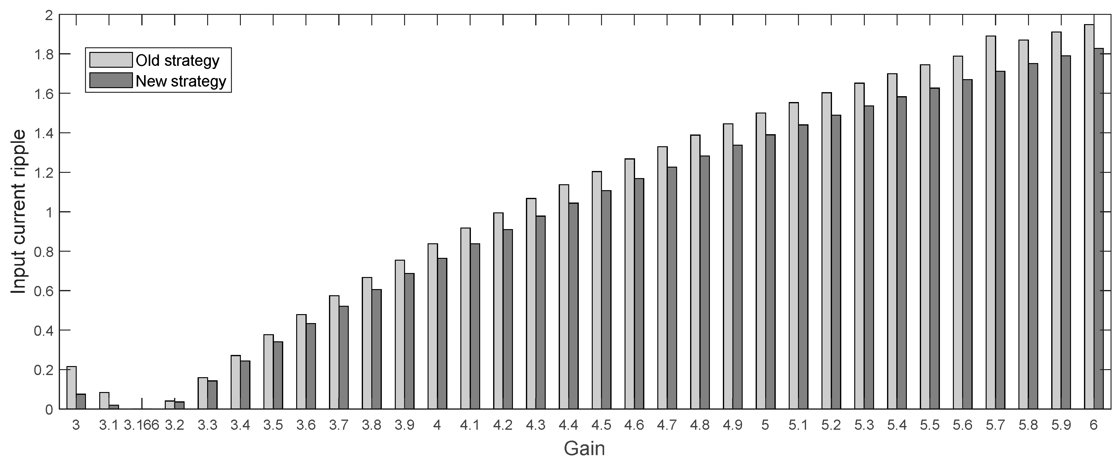
Results obtained by the former strategy are reported in

Table 2. Comparative table of the obtained results with the former and the proposed strategy.

Strategy	G	D	k	Δig	IL1	IL2
Former	3.0	0.5785	0.6666	0.2154	1.6277	1.3722
Proposed		0.5807	0.6751	0.0756	1.6611	1.3987
Former	3.1	0.5916	0.6666	0.0838	1.7063	1.4970
Proposed		0.5951	0.6687	0.0195	1.7333	1.5338
Former	3.166¯	0.6000	0.6666	0.0000	1.7593	1.5833
Proposed		0.6000	0.6666	0.0000	1.7593	1.5833
Former	3.2	0.6041	0.6666	0.0408	1.7859	1.6275
Proposed		0.6036	0.6686	0.0365	1.7880	1.6239
Former	3.3	0.6159	0.6666	0.1589	1.8663	1.7638
Proposed		0.6143	0.6743	0.1428	1.8777	1.7519
Former	3.4	0.6271	0.6666	0.2709	1.9475	1.9058
Proposed		0.6244	0.6796	0.2441	1.9685	1.8838
Former	3.5	0.6377	0.6666	0.3773	2.0295	2.0537
Proposed		0.6341	0.6845	0.3408	2.0613	2.0218
Former	3.6	0.6479	0.6666	0.4785	2.1123	2.2076
Proposed		0.6433	0.6890	0.4331	2.1550	2.1639
Former	3.7	0.6575	0.6666	0.5749	2.1958	2.3675
Proposed		0.6521	0.6932	0.5213	2.2503	2.3113
Former	3.8	0.6667	0.6666	0.6667	2.2800	2.5334
Proposed		0.6605	0.6971	0.6057	2.3469	2.4636
Former	3.9	0.6754	0.6666	0.7542	2.3648	2.7052
Proposed		0.6686	0.7008	0.6864	2.4456	2.6222
Former	4	0.6838	0.6666	0.8377	2.4503	2.8830
Proposed		0.6764	0.7042	0.7638	2.5460	2.7868
Former	4.1	0.6917	0.6666	0.9175	2.5363	3.0670
Proposed		0.6838	0.7074	0.8380	2.6468	2.9551
Former	4.2	0.6994	0.6666	0.9938	2.6230	3.2570
Proposed		0.6909	0.7104	0.9093	2.7489	3.1286
Former	4.3	0.7067	0.6666	1.0668	2.7102	3.4533
Proposed		0.6977	0.7133	0.9777	2.8525	3.3071
Former	4.4	0.7137	0.6666	1.1367	2.7979	3.6557
Proposed		0.7043	0.7159	1.0435	2.9574	3.4923
Former	4.5	0.7204	0.6666	1.2036	2.8859	3.8640
Proposed		0.7106	0.7185	1.1067	3.0638	3.6820
Former	4.6	0.7268	0.6666	1.2678	2.9746	4.0787
Proposed		0.7167	0.7209	1.1676	3.1716	3.8781
Former	4.7	0.7329	0.6666	1.3294	3.0636	4.2997
Proposed		0.7226	0.7231	1.2262	3.2805	4.0803
Former	4.8	0.7389	0.6666	1.3885	3.1531	4.5267
Proposed		0.7282	0.7253	1.2827	3.3900	4.2854
Former	4.9	0.7445	0.6666	1.4454	3.2431	4.7604
Proposed		0.7337	0.7273	1.3371	3.5017	4.4995
Former	5	0.7500	0.6666	1.5000	3.3333	5.0000
Proposed		0.7389	0.7292	1.3896	3.6125	4.7149
Former	5.1	0.7553	0.6666	1.5526	3.4241	5.2462
Proposed		0.7440	0.7311	1.4403	3.7268	4.9396
Former	5.2	0.7603	0.6666	1.6031	3.5149	5.4982
Proposed		0.7489	0.7328	1.4893	3.8406	5.1684
Former	5.3	0.7652	0.6666	1.6518	3.6063	5.7567
Proposed		0.7536	0.7345	1.5366	3.9555	5.4014
Former	5.4	0.7699	0.6666	1.6988	3.6980	6.0220
Proposed		0.7582	0.7361	1.5824	4.0724	5.6428
Former	5.5	0.7744	0.6666	1.7441	3.7901	6.2936
Proposed		0.7626	0.7377	1.6266	4.1899	5.8875
Former	5.6	0.7788	0.6666	1.7877	3.8822	6.5710
Proposed		0.7669	0.7391	1.6694	4.3080	6.1397
Former	5.7	0.7830	0.6666	1.8899	3.9749	6.8555
Proposed		0.7711	0.7405	1.7109	4.4287	6.4003
Former	5.8	0.7871	0.6666	1.8706	4.0677	7.1461
Proposed		0.7751	0.7419	1.7510	4.5492	6.6626
Former	5.9	0.7910	0.6666	1.9099	4.1608	7.4429
Proposed		0.7790	0.7432	1.7899	4.6708	6.9322
Former	6	0.7948	0.6666	1.9479	4.2541	7.7462
Proposed		0.7827	0.7444	1.8276	4.7904	7.2014

. The best outcomes are highlighted in boldface. A close inspection in Table 2 demonstrates that the new strategy achieves the lowest input current ripple Δ_ig in all experiments, and also proves a better balance in the power-sharing among converters than the old strategy.

Figure 7 shows the reported values in Table 2. From this figure, it is evident how the new strategy achieves lower values for the input current ripple in the full operating range. An exception occurs when the gain G is 3.166¯. In that case, both methods reach the same minimum value for the input current ripple.

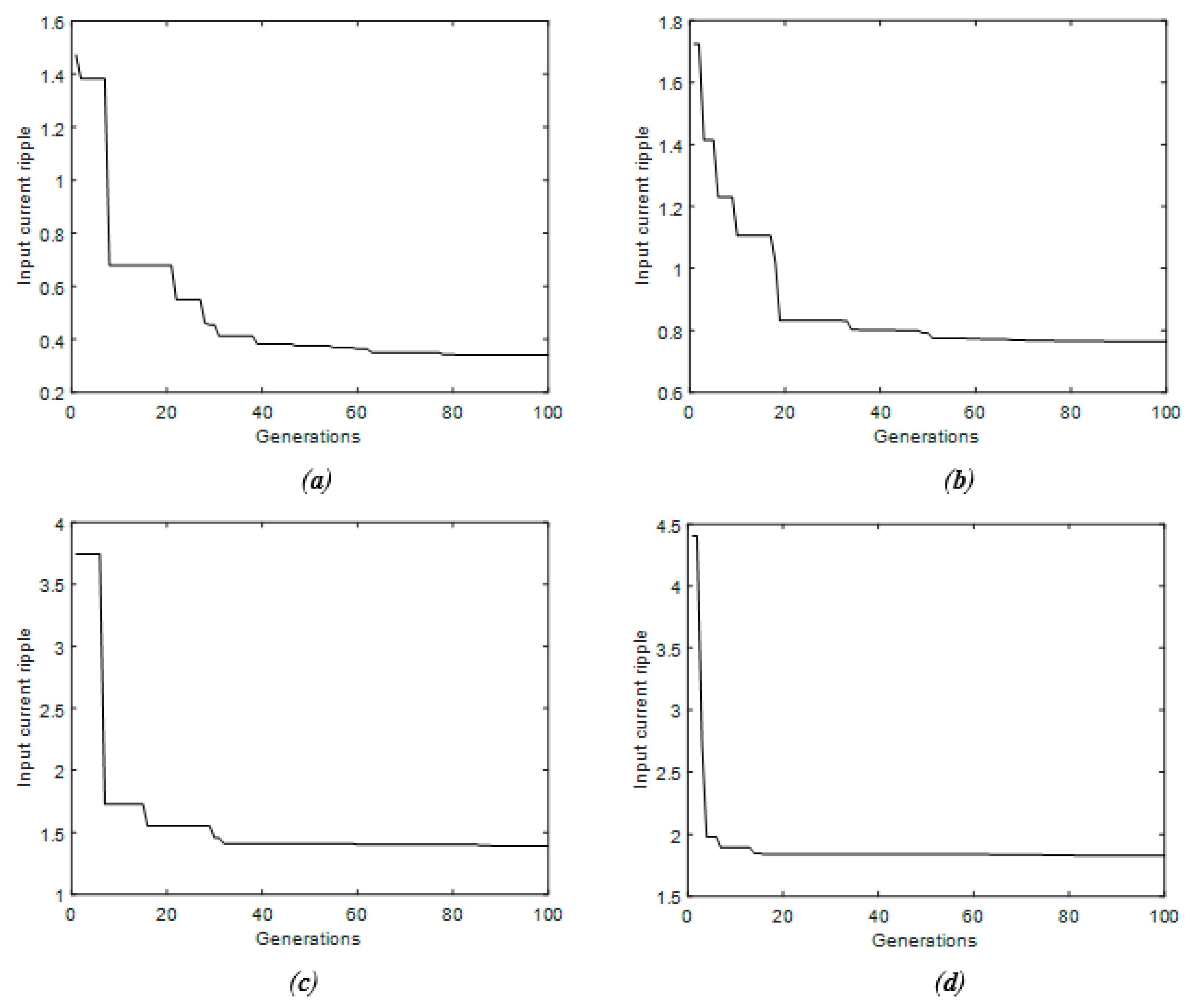
A convergence-graph is presented in Figure 8 to evaluate the speed performance of the DE algorithm. In the test, four operation points are considered to analyze the velocity of the optimization algorithm in reaching the optimal value. This figure shows, in a single execution, the obtained input current ripple in every generation, where the considered gains are 3.5, 4, 5, and 6 for Figure 8a–d, respectively. These gain values have been selected according to the most representative and significant operation points.

The reported results have been validated and analyzed under a statistical context. In the analysis, the Wilcoxon test has been implemented [32] to determine the difference between both strategies in comparison. A null hypothesis is established in the Wilcoxon test, in which there is no evidence that indicates a significant difference among both approaches. On the other hand, the null hypothesis is rejected when a significant difference is observable.

Additionally, the Wilcoxon test considering one sample has been conducted to determine if the median value of the proposed strategy is significantly lower than the hypothesized median value of the former method for each operating point. A null hypothesis is established in which there is no evidence that indicates the median value of the proposed method is significantly lower than the hypothesized median value of the former strategy. This test will statistically confirm if our approach reaches a lower input current ripple than the old strategy.

In both analyses, the 30 Δ_ig results obtained from 30 independent executions for each operation point are contemplated as the observations of the proposed strategy. Regarding the former strategy, the obtained result Δ_ig is considered 30 times since it always reaches the same value for every operating point. The Wilcoxon statistic and the p-values obtained from both tests in every operating point indicate if the null hypothesis has been accepted or rejected. Therefore, if the p-values are lower than the significance level of 0.05, the null hypothesis is rejected.

The obtained p-values for two samples are lower than the significance level, reaching a p-value of 0.0000639 in all operating points. Statistically, these values are too small, so they can be considered zero. Besides, the obtained p-values are the same in all operating points because the 30 observations of each configuration are lower than the hypothesized median value of the former strategy, causing the median value of the proposed method to be lower than the hypothesized median. Except for G=3.166¯, where all observations are higher, causing the median value of the proposed method to be higher than the hypothesized median. Both scenarios generate the same p-values and indicate a significant difference between the approaches in comparison. Summarizing, the obtained p-values for two samples confirm that there is evidence against the null hypothesis, indicating a significant difference among both approaches for all the numerical experiments.

Similarly, the p-values for one sample are lower than the significance level, reaching a p-value of 0.000032 in all operating points. These results confirm that there is evidence against the null hypothesis, indicating that our approach reaches a lower input current ripple than the old strategy for all the numerical experiments. An exception occurs when G = 3.166¯, where the null hypothesis is accepted. In this case, all observations were higher than the hypothesized median value of the former strategy, which can be confirmed by the corresponding Wilcoxon statistic, whose value is 465. This means that the new approach did not achieve a lower input current ripple than the old method for this operating point, and can be confirmed by observing the reported Δ_ig value from Table 2 for G = 3.166¯, where both approaches reached the same input current ripple.

Considering the statistical results, we can conclude that the Wilcoxon test supports the reported outcomes from Table 2, in which the proposed strategy has demonstrated its superiority against the former strategy.

As a complementary analysis, the speed performance of the algorithms is presented. For the proposed method, 30 independent executions have been considered. The experiments have been implemented on a PC with 8 GB of memory and an Intel^® Core i7 Processor (3.4 GHz).

From the speed test, the elapsed real-time of the former strategy ranges from 0.01 to 0.02 s. These variations are due to delays in the internal computation process. On the other hand, the proposed method differs from 0.19 to 0.21 s because of the same reason. These variations are bigger than those reported by the old strategy because the new approach requires more calculus, causing more delays.

Summarizing, it is evident that the former strategy is faster than the proposed method. As it was expected, our approach requires more computational time to find the optimal duty cycle combination. However, the execution time is approximately 20% of one second, which is quite fast, considering that the new strategy is an iterative method.

7. Discussion

As shown in Table 2, the former strategy provides a large current ripple for all operation points, except with the zero ripple operation point, in which both strategies provide zero input current ripple. Furthermore, the power-sharing among power stages is more balanced (the current among inductors has less difference).

One compromise of the optimization is evidently the time it takes to optimize (minimize the input current ripple), the former strategy takes less time to choose the duty cycle, but the input current-ripple is not optimized. In a real application there are two choices to implement the optimized duty cycle, the first option would be to calculate off-line the optimized k for each duty cycle, and chose the consequent k from a look-up table, a second options, which depends on the application, is to have a microcontroller (a small microprocessor), to run the DE algorithm online, the advantage of the second option it would be to have a better optimization in the case the duty cycle is in between two duty cycles of the look-up table, it would be better to optimize it again, instead of doing the linear interpolation, in the other hand, it would require more computational power from the control system of the converter.

8. Conclusions

This article introduced a new PWM strategy for the hybrid interleaved boost-Cuk converter, the proposed strategy uses the differential evolution (DE) algorithm to find the duty cycle and the scalar factor k, which defines the duty cycle of each interleaved stage in an independent manner, the algorithm fulfills the required gain, and at the same time, it minimizes the input current ripple. It is shown that the proposed method achieves a smaller input current ripple in the full operation range compared against the input current ripple for the former strategy, which already had a low input current ripple, the proposed approach also provides a better (more balanced) power-sharing among converters. Although the proposed method is computationally more expensive than the former strategy, the obtained duty cycle combination significantly decreases the input current ripple, which satisfies one of the most desired characteristics for a converter, in which a non-pulsating input current with low ripple is achieved. Otherwise, a pulsating current or current with higher ripple produces an early aging of the renewable energy source because the root-mean-square value of the current is larger, generating additional power conduction.

As future work, the performance analysis of other evolutionary algorithms for the duty cycle optimization problem can be conducted. This research will provide valuable information on selecting the best optimization option. Furthermore, the mathematical model can be improved by a possible merging of constraints in order to allow finding a lower ripple by the evolutionary algorithm.

References

- Erickson, R.W.; Maksimovic, D. Fundamentals of Power Electronics, 2nd ed.; Kluwer: New York, NY, USA, 2001. [Google Scholar]
- Thounthong, P.; Davat, B.; Rael, S.; Sethakul, P. Fuel cell high-power applications. IEEE Ind. Electron. Mag. 2009, 3, 32–46. [Google Scholar]
- Wang, C. Investigation on interleaved boost converters and applications. Ph.D. Dissertation, Virginia Polytechnic Institute and State University, Blacksburg, VA, USA, July 2009. [Google Scholar]
- Jang, Y.; Jovanovic, M.M. Interleaved Boost Converter with Intrinsic Voltage-Doubler Characteristic for Universal-Line PFC Front End. IEEE Trans. Power Electron. 2007, 22, 1394–1401. [Google Scholar] [CrossRef]
- Arias-Angulo, J.P.; Rosas-Caro, J.C.; Beltran-Carbajal, F.; Valderrabano-Gonzalez, A.; Haro-Sandoval, E.; Gutierrez-Alcala, S.; Alejo-Reyes, A.; Garcia-Vite, P.M. Power quality improvement by interleaving unequal switching converters. IEICE Electron. Express 2016, 13, 20160558. [Google Scholar]
- Storn, R.; Price, K. Differential Evolution–A Simple and Efficient Heuristic for global Optimization over Continuous Spaces. J. Glob. Optim. 1997, 11, 341–359. [Google Scholar] [CrossRef]
- Holland, J.H. Adaptation in Natural and Artificial Systems; University of Michigan Press: Ann Arbor, MI, USA, 1975. [Google Scholar]
- Eberhart, R.; Kennedy, J. A New Optimizer Using Particle Swarm Theory; MHS’95. In Proceedings of the Sixth International Symposium on Micro Machine and Human Science, Nagoya, Japan, 4–6 October 1995; pp. 39–43. [Google Scholar]
- Zaldívar, D.; Morales, B.; Rodríguez, A.; Valdivia-G, A.; Cuevas, E.; Pérez-Cisneros, M. A novel bio-inspired optimization model based on Yellow Saddle Goatfish behavior. BioSystems 2018, 174, 1–21. [Google Scholar] [CrossRef] [PubMed]
- Viktorin, A.; Senkerik, R.; Pluhacek, M.; Kadavy, T.; Zamuda, A. Distance based parameter adaptation for Success-History based Differential Evolution. Swarm Evol. Comput. 2019, 50. [Google Scholar] [CrossRef]
- Leboucher, C.; Shin, H.S.; Chelouah, R.; Stephane, L.M.; Siarry, P.; Formoso, M.; Tsourdos, A.; Kotenkoff, A. An Enhanced Particle Swarm Optimization Method Integrated With Evolutionary Game Theory. IEEE Trans. Games 2018, 10, 221–230. [Google Scholar] [CrossRef]
- Awad, N.H.; Ali, M.Z.; Suganthan, P.N. Ensemble sinusoidal differential covariance matrix adaptation with Euclidean neighborhood for solving CEC2017 benchmark problems. In Proceedings of the 2017 IEEE Congress on Evolutionary Computation (CEC) Proceedings, Donostia-San Sebastián, Spain, 5–8 June 2017; pp. 372–379. [Google Scholar]
- Kaur, K.; Singh, U.; Salgotra, R. An enhanced moth flame optimization. In Neural Computing and Applications; Springer: Berlin, Germany, 2018. [Google Scholar] [CrossRef]
- Lynn, N.; Suganthan, P.N. Heterogeneous comprehensive learning particle swarm optimization with enhanced exploration and exploitation. Swarm Evol. Comput. 2015, 24, 11–24. [Google Scholar] [CrossRef]
- Gao, H.; Shi, Y.; Pun, C.M.; Kwong, S. An Improved Artificial Bee Colony Algorithm with its Application. IEEE Trans. Ind. Inform. 2019, 15, 1853–1865. [Google Scholar] [CrossRef]
- Lynn, N.; Suganthan, P.N. Ensemble particle swarm optimizer. Appl. Soft Comput. 2017, 55, 533–548. [Google Scholar] [CrossRef]
- Cai, Z.; Niu, J.; Yang, X. A Multi Measure Improved Firefly Algorithm. In Proceedings of the 2018 2nd IEEE Advanced Information Management, Communicates, Electronic and Automation Control Conference 2018, Xian, China, 23–23 March 2018; pp. 20–26. [Google Scholar]
- Banerjee, S.; Ghosh, A.; Rana, N. An Improved Interleaved Boost Converter With PSO-Based Optimal Type-III Controller. IEEE J. Emerg. Sel. Top. Power Electron. 2017, 5, 323–337. [Google Scholar] [CrossRef]
- Suganya, R.; Rajkumar, M.V.; Pushparani, P. Simulation and Analysis of Boost Converter with MPPT for PV System using Chaos PSO Algorithm. Int. J. Emerg. Technol. Eng. Res. 2017, 5, 97–105. [Google Scholar]
- Laoprom, I.; Tunyasrirut, S. Design of PI Controller for Voltage Controller of Four-Phase Interleaved Boost Converter Using Particle Swarm Optimization. J. Control Sci. Eng. 2020, 2020, 9515160. [Google Scholar] [CrossRef] [Green Version]
- Yang, S.; Qing, A. Design of high-Power Millimeter-wave TM/sub 01/-TE/sub 11/Mode converters by the differential evolution algorithm. IEEE Trans. Plasma Sci. 2005, 33, 1372–1376. [Google Scholar] [CrossRef]
- Zhang, D.; Liu, Y.; Huang, S. Differential Evolution Based Parameter Identification of Static and Dynamic J-A Models and Its Application to Inrush Current Study in Power Converters. IEEE Trans. Magn. 2012, 48, 3482–3485. [Google Scholar] [CrossRef]
- Taheri, H.; Salam, Z.; Ishaque, K.; Syafaruddin. A novel Maximum Power Point tracking control of photovoltaic system under partial and rapidly fluctuating shadow conditions using Differential Evolution. In Proceedings of the 2010 IEEE Symposium on Industrial Electronics and Applications (ISIEA), Penang, Malaysia, 3–6 October 2010; pp. 82–87. [Google Scholar]
- Yahia, H.; Liouane, N.; Dhifaoui, R. Weighted differential evolution based PWM optimization for single phase voltage source inverter. Int. Rev. Electr. Eng. 2010, 5, 1956–1962. [Google Scholar]
- Mohd-Rashid, M.I.; Hiendro, A.; Anwari, M. Optimal HE-PWM inverter switching patterns using differential evolution algorithm. In Proceedings of the 2012 IEEE International Conference on Power and Energy (PECon), Kota Kinabalu, Malaysia, 2–5 December 2012; pp. 32–37. [Google Scholar]
- Slowik, A.; Kwasnicka, H. Nature Inspired Methods and Their Industry Applications—Swarm Intelligence Algorithms. IEEE Trans. Ind. Inform. 2018, 14, 1004–1015. [Google Scholar] [CrossRef]
- Dulebenets, M.A. A Comprehensive Evaluation of Weak and Strong Mutation Mechanisms in Evolutionary Algorithms for Truck Scheduling at Cross-Docking Terminals. IEEE Access 2018, 6, 65635–65650. [Google Scholar] [CrossRef]
- Dulebenets, M.A. A Delayed Start Parallel Evolutionary Algorithm for Just-in-Time Truck Scheduling at a Cross-Docking Facility. Int. J. Prod. Econ. 2019, 212, 236–258. [Google Scholar] [CrossRef]
- Zhao, X.; Wang, C.; Su, J.; Wang, J. Research and Application Based on the Swarm Intelligence Algorithm and Artificial Intelligence for Wind Farm Decision System. Renew. Energy 2019, 134, 681–697. [Google Scholar] [CrossRef]
- Brezočnik, L.; Fister, I.; Podgorelec, V. Swarm Intelligence Algorithms for Feature Selection: A Review. Appl. Sci. 2018, 8, 1521. [Google Scholar] [CrossRef] [Green Version]
- Anandakumar, H.; Umamaheswar, K. A Bio-Inspired Swarm Intelligence Technique for Social Aware Cognitive Radio Handovers. Comput. Electr. Eng. 2018, 71, 925–937. [Google Scholar] [CrossRef]
- Wilcoxon, F. Individual Comparisons by Ranking Methods. Biom. Bull. 1945, 1, 80–83. [Google Scholar] [CrossRef]
Figure 1.
The traditional boost converter, and important waveforms related to the input current ripple.
Figure 2.
The (two phases) traditional interleaved boost converter (a) topology and PWM generation strategy, (b) important waveforms related to the input current ripple.
Figure 3.
The hybrid converter proposes in [5], (a) topology, (b) switching functions generation strategy and waveforms related to the PWM, (c) important waveforms related to the input current ripple.
Figure 4.
PWM important waveforms in the proposed converter when D > DZ.
Figure 5.
PWM important waveforms in the proposed converter when D < DZ.
Figure 6.
Flowchart of the differential evolution (DE) algorithm.
Figure 7.
Comparison of the obtained results with the old and new strategy for different operation points.
Figure 8.
Convergence graph of the DE algorithm for (a) G = 3.5, (b) G = 4, (c) G = 5, and (d) G = 6.