Analysis of the Past Lifetime in a Replacement Model through Stochastic Comparisons and Differential Entropy

Abstract

A suitable replacement model for random lifetimes is extended to the context of past lifetimes. At a fixed time u an item is planned to be replaced by another one having the same age but a different lifetime distribution. We investigate the past lifetime of this system, given that at a larger time t the system is found to be failed. Subsequently, we perform some stochastic comparisons between the random lifetimes of the single items and the doubly truncated random variable that describes the system lifetime. Moreover, we consider the relative ratio of improvement evaluated at $x\in (u,t)$, which is finalized to measure the goodness of the replacement procedure. The characterization and the properties of the differential entropy of the system lifetime are also discussed. Finally, an example of application to the firing activity of a stochastic neuronal model is provided.

1. Introduction

The problem of the reliability and survival analysis of a system has been widely studied in recent years. In various cases, the availability of the system is improved by means of replacements or duplications of the involved subsystems. Indeed, a typical problem in Engineering Reliability is the determination of a suitable policy for the replacement or the improvement of the system components. The literature is quite large in this area, as an example we refer to Jardine and Tsang [1] and Thomas [2].

In some cases, the reliability of a system is analyzed on the ground of partially available information that is concerning the status of the system or its components at certain fixed instants. In these instances, it is necessary to study the reliability measures of interest under the condition of truncated or doubly truncated random variables. In this contribution, we refer to a previous investigation centered on a stochastic model dealing with the replacement of items occurring at deterministic arbitrary instants (see Di Crescenzo and Di Gironimo [3]). We aim to generalize this model, by assuming that a given item is replaced by another item at a fixed instant, in such a way that their lifetimes have the same age but possess different distributions. Afterwards, we assume that, at a subsequent fixed inspection time, the system is found to be failed. Thus, we investigate the corresponding past lifetime within the considered replacement model. Hence, differently from the previous investigation, which was centered on the residual lifetime, in this case we focus on the past lifetime of the system. Due to the nature of the treated model, specific attention is given to the reversed hazard rate, and to related stochastic quantities, since this measure is particularly suitable in the context of lifetimes conditioned on lower intervals. A special role, in this case, is played by the double truncation of the considered random lifetimes, in order to measure the time elapsed from the failure of the first item up to a fixed time instant.

We recall that classical results on allocation of redundant items in systems, and construction of relevation models are contained in various contributions, such as Krakowski [4]. Here, the author introduced the study of a system that describes the overall lifetime of a component, which is replaced at its (random) failure time by another component of the same age, whose lifetime distribution is possibly different. In this research area, we also recall Baxter [5], Sordo and Psarrakos [6], Belzunce et al. [7], and [8].

The topic of double truncation of random lifetimes has been treated in the reliability literature first by Navarro and Ruiz [9], and Ruiz and Navarro [10,11], through an extension of the failure rate. In this framework, other results have been centered on properties of the expected value (cf. Sankaran and Sunoj [12]) and of the conditional expectations (see Su and Huang [13], Ahmad [14], Betensky and Martin [15], Navarro and Ruiz [16], Bairamov and Gebizlioglu [17], Poursaeed and Nematollahi [18], and Sunoj et al. [19]). We also recall the analysis of the doubly truncated mean residual lifetime and the doubly truncated mean past to failure performed by Khorashadizadeh et al. [20].

The main aim of this paper is to investigate the effect of the replacement, with attention to criteria that lead to a better system performance. The mathematical tools used in our investigation involve stochastic orders and other reliability notions, such as the past lifetime. Moreover, the past entropy is employed to encompass the relevant informational properties. We recall various investigation in this area, due to Di Crescenzo and Longobardi [21], Di Crescenzo and Toomaj [22], Kundu and Nanda [23], Kundu et al. [24], and Nanda and Paul [25].

In order to illustrate the effect of the replacement in a context of interest in theoretical neurobiology, in this paper we also investigate an application to a solvable stochastic neuronal model.

The paper is organized as follows. Section 2 is devoted to introduce the replacement stochastic model and the main quantities of interest, including its past lifetime, the hazard rate, and the reversed hazard rate. In Section 3, we perform some stochastic comparisons, and show how the existence of suitable orderings between the lifetimes involved in the replacement mechanism affects the same orderings for the system lifetime. We also illustrate some related examples. Further comparisons are treated in Section 4, based on the case when the replacement rule involves random variables having the same distribution. The analysis is performed by resorting to the double past lifetime of the system. Specifically, we stochastically compare the double random variables and their expected values. Section 5 deals with the relative ratio of improvement for the considered model and its properties. We also provide an example involving exponentially distributed random lifetimes. In Section 6, we obtain various results concerning the differential entropy of the system lifetime for the considered model. These are based on the determination of the differential entropy of the double random past lifetime and on related stochastic comparisons. In Section 7, we provide the announced application to neuronal dynamics. Finally, some concluding remarks are provided in Section 8.

2. The Model

Let X be an absolutely continuous nonnegative random variable with cumulative distribution function (CDF) $F(x)=\mathbb{P}(X\le x)$, probability density function (PDF) $f(x)$, survival function $\overline{F}(x)=1-F(x)$. Bearing in mind possible applications to reliability theory and survival analysis, we assume that X describes the random lifetime of an item or a living organism. Let us now recall two functions of interest; as usual we denote by

$${\lambda }_X(x)=-\frac{\mathrm{d}}{\mathrm{d}x}log\overline{F}(x)=\frac{f(x)}{\overline{F}(x)},x\in {ℝ}_{+},\overline{F}(x)>0$$

the hazard rate (or failure rate) of X, and by

$$r_X(x)=\frac{\mathrm{d}}{\mathrm{d}x}logF(x)=\frac{f(x)}{F(x)},x\in {ℝ}_{+},F(x)>0$$

the reversed hazard rate function of X.

See Barlow and Proschan [26] and Block et al. [27] for some illustrative results on these notions. Denote by Y another absolutely continuous nonnegative random variable with CDF $G(x)$, PDF $g(x)$, survival function $\overline{G}(x)$, hazard rate ${\lambda }_Y(x)$, and reversed hazard rate $r_Y(x)$.

We assume that X and Y are independent lifetimes of two suitable items. Both items start working at time 0. A replacement of the first item by the second one (having the same age) is planned to occur at time $u>0$, provided that the first item is not failed before. Assume that at the inspection time $t>u$, the system is found to be failed. We denote by $X_{u,t}^{(Y)}$ the random past lifetime of the system, which can be expressed as

$$X_{u,t}^{(Y)}=\left\{\begin{array}{cc}[X|X\le u]\hfill & \mathrm{if}0\le X\le u\hfill \\ [Y|u<Y\le t]\hfill & \mathrm{if}X>u.\hfill \end{array}\right.$$

(1)

Indeed, we take into account that, at time $t>u$, the system is inspected and it is found failed. If the first item has failed before the replacement time u, and then the system lifetime is equal to the lifetime of first item. Otherwise, if the first item is replaced at time u, then the system lifetime is equal to the lifetime of the second unit.

According to Equation (1), throughout the paper we implicitly assume that $\mathbb{P}(u<Y\le t)>0$, i.e., $G(u)<G(t)$ for fixed $0<u<t$. Moreover, for any Borel set B, and for all $0<u<t$, we have the following relation:

$$\mathbb{P}(X_{u,t}^{(Y)}\in B)=\mathbb{P}(X\in B|X\le u)F(u)+\mathbb{P}(Y\in B|u<Y\le t)\overline{F}(u).$$

In particular, if $B=(0,x]$ one has

$$\mathbb{P}(X_{u,t}^{(Y)}\le x)=\mathbb{P}(X\le x|X\le u)F(u)+\mathbb{P}(Y\le x|u<Y\le t)\overline{F}(u).$$

Hence, the CDF of $X_{u,t}^{(Y)}$ is expressed as

$$F_{u,t}^{(Y)}(x):=\mathbb{P}(X_{u,t}^{(Y)}\le x)=\left\{\begin{array}{cc}F(x)\hfill & \mathrm{if}0\le x\le u\hfill \\ {\displaystyle F(u)+\frac{G(x)-G(u)}{G(t)-G(u)}\overline{F}(u)}\hfill & \mathrm{if}u<x\le t\hfill \\ 1\hfill & \mathrm{if}x\ge t,\hfill \end{array}\right.$$

(2)

and the corresponding PDF reads

$${\displaystyle f_{u,t}^{(Y)}(x)=\frac{\mathrm{d}}{\mathrm{d}x}{F}_{u,t}^{(Y)}(x)=\left\{\begin{array}{cc}f(x)\hfill & \mathrm{if}0\le x\le u\hfill \\ {\displaystyle \frac{g(x)}{G(t)-G(u)}\overline{F}(u)}\hfill & \mathrm{if}u<x\le t.\hfill \end{array}\right.}$$

(3)

Consequently, the survival function of $X_{u,t}^{(Y)}$ is defined by

$${\overline{F}}_{u,t}^{(Y)}(x)=\mathbb{P}(X_{u,t}^{(Y)}>x)=\left\{\begin{array}{cc}\overline{F}(x)\hfill & \mathrm{if}0\le x\le u\hfill \\ {\displaystyle \overline{F}(u)\frac{G(t)-G(x)}{G(t)-G(u)}}\hfill & \mathrm{if}u<x\le t\hfill \\ 0\hfill & \mathrm{if}x\ge t.\hfill \end{array}\right.$$

(4)

Let us now give the hazard rate of $X_{u,t}^{(Y)}$

$${\lambda }_{u,t}^{(Y)}(x)=\frac{f_{u,t}^{(Y)}(x)}{{\overline{F}}_{u,t}^{(Y)}(x)}=\left\{\begin{array}{cc}{\lambda }_X(x)\hfill & \mathrm{if}0\le x\le u\hfill \\ {\displaystyle \frac{g(x)}{G(t)-G(x)}}\hfill & \mathrm{if}u<x<t,\hfill \end{array}\right.$$

(5)

and its reversed hazard rate

$$r_{u,t}^{(Y)}(x)=\frac{f_{u,t}^{(Y)}(x)}{F_{u,t}^{(Y)}(x)}=\left\{\begin{array}{cc}{r}_X(x)\hfill & \mathrm{if}0<x\le u\hfill \\ {\displaystyle \frac{g(x)\overline{F}(u)}{F(u)[G(t)-G(x)]+G(x)-G(u)}}\hfill & \mathrm{if}u<x\le t.\hfill \end{array}\right.$$

(6)

We remark that the functions that are given in (5) and (6) are not necessarily continuous at $x=u$. Moreover, we have ${\lambda }_{u,t}^{(Y)}(x)\to +\infty$ for $x\to t$.

Hereafter, we provide a brief example of interest in industrial engineering.

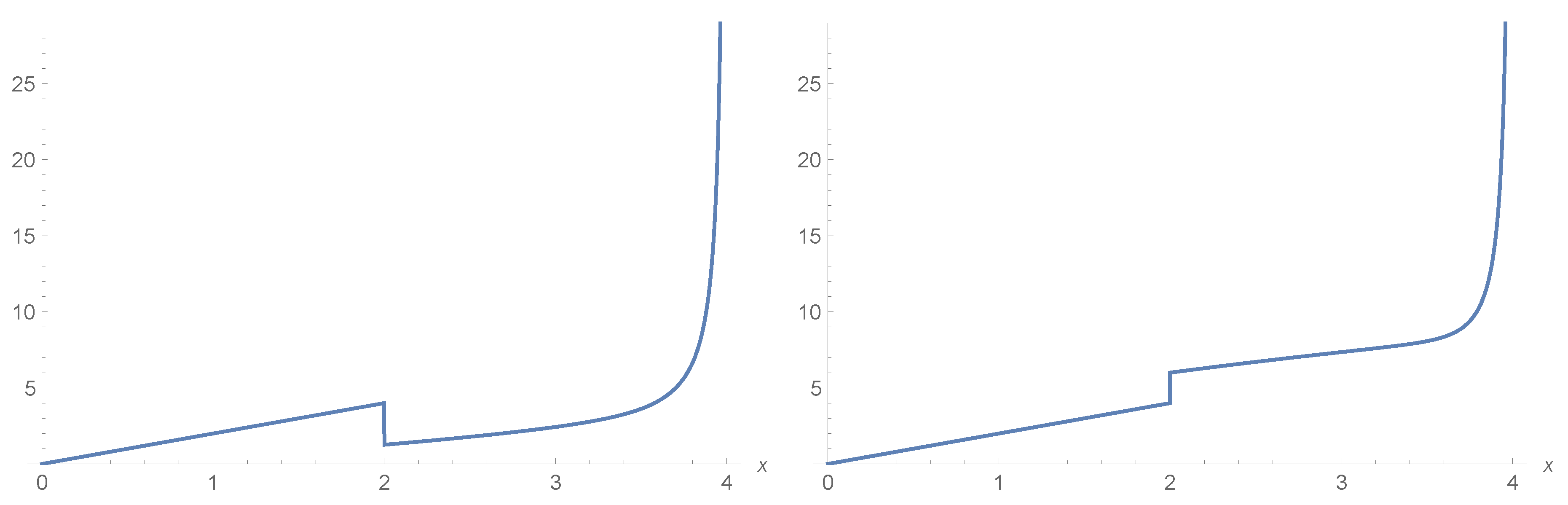
Example 1.

Let X and Y be independent lifetimes of two items, having Weibull distribution, with $F(x)=1-e^{-{(x/\lambda )}^k}$, $x\ge 0$, and $G(x)=1-e^{-{(x/\mu )}^h}$, $x\ge 0$, for $\lambda ,k,\mu ,h>0$. According to the assumptions given above, we assume that a replacement of the first item by the second one is planned at time $u>0$, and that at time $t>u$ an inspection finds the system failed. Clearly, the replacement produces a modification in the system reliability. As example, in Figure 1 we show the system hazard rate (5) in two different cases. In both cases, at time $u=2$ the hazard rate performs a jump. In the first case the jump is downward, since X is smaller than Y in the usual stocastic order (see Definition 1), which means that, at time u, the first item is replaced by a more reliable item. On the contrary, in the second case the jump is upward, since the condition on the items is reversed.

3. Stochastic Comparisons

In the following, we recall some useful definitions and comparison properties of $X,Y$ with $X_{u,t}^{(Y)}$. We refer to [28] or [29] for more details. Note that the terms increasing and decreasing are used in a non-strict sense.

Definition 1.

Let X be an absolutely continuous random variable with support $(l_X,u_X)$, CDF F, and PDF f. Similarly, let Y be an absolutely continuous random variable with support $(l_Y,u_Y)$, CDF G, and PDF g. We say that X is smaller than Y in the

(a) 

usual stocastic order ($X{\le }_{\mathrm{st}}Y$) if $\overline{F}(t)\le \overline{G}(t)\forall t\in ℝ$ or, equivalently, if $F(t)\ge G(t)$ $\forall t\in ℝ$;

(b) 

hazard rate order ($X{\le }_{\mathrm{hr}}Y$) if $\overline{G}(t)/\overline{F}(t)$ increases in $t\in (-\infty ,max(u_X,u_Y))$ or, equivalently, if ${\lambda }_X(t)\ge {\lambda }_Y(t)$ for all $t\in ℝ$, where ${\lambda }_X(t)=f(t)/\overline{F}(t)$ and ${\lambda }_Y(t)=g(t)/\overline{G}(t)$ are, respectively, the hazard rates of X and Y, or equivalently if $f(x)\overline{G}(y)\ge g(x)\overline{F}(y)$ $\forall x\le y$;

(c) 

likelihood ratio order ($X{\le }_{\mathrm{lr}}Y$) if $f(x)g(y)\ge f(y)g(x)$ for all $x\le y$, with $x,y\in (l_X,u_X)\cup (l_Y,u_Y)$ or, equivalently, $g(t)/f(t)$ increases in t over the union of supports of X and Y;

(d) 

reversed hazard rate order ($X{\le }_{\mathrm{rh}}Y$) if $G(t)/F(t)$ increases in $t\in (min(l_X,l_Y),+\infty )$.

We recall the following relations among the above defined stochastic orders:

$$X{\le }_{\mathrm{lr}}Y\Rightarrow X{\le }_{\mathrm{hr}}Y\Rightarrow X{\le }_{\mathrm{st}}Y,X{\le }_{\mathrm{lr}}Y\Rightarrow X{\le }_{\mathrm{rh}}Y\Rightarrow X{\le }_{\mathrm{st}}Y.$$

(7)

Now, we study the effect of replacement when the lifetime of the first item is stochastically smaller than the second in the sense of Definition 1.

Theorem 1.

Let X and Y be absolutely continuous nonnegative random variables. Subsequently,

(i) $X{\le }_{\mathrm{hr}}Y$ ⇒ $X_{u,t}^{(Y)}{\le }_{\mathrm{hr}}Y$ $\forall 0<u<t$;

(ii) $X{\le }_{\mathrm{st}}Y$ ⇒ $X_{u,t}^{(Y)}{\le }_{\mathrm{st}}Y$ $\forall 0<u<t$.

Proof. 

Being

$${\lambda }_{u,t}^{(Y)}(x)=\frac{f_{u,t}^{(Y)}(x)}{{\overline{F}}_{u,t}^{(Y)}(x)}=\left\{\begin{array}{cc}{\lambda }_X(x)\hfill & \mathrm{if}0\le x\le u\hfill \\ {\displaystyle \frac{g(x)}{G(t)-G(x)}}\hfill & \mathrm{if}u<x\le t,\hfill \end{array}\right.$$

we easily have that ${\lambda }_{u,t}^{(Y)}(x)={\lambda }_X(x)\ge {\lambda }_Y(x)$ for all $0\le x\le u$, and

$${\lambda }_{u,t}^{(Y)}(x)=\frac{g(x)}{G(t)-G(x)}\ge \frac{g(x)}{1-G(x)}={\lambda }_Y(x)\forall u<x\le t,$$

this giving the proof of (i).

Concerning point (ii), from (4) the case $0\le x\le u$ is immediate. In the second case, we have

$$0\le \overline{G}(t)[\overline{G}(u)-\overline{G}(x)]=\overline{G}(t)[\overline{F}(u)-\overline{G}(x)]+\overline{G}(t)[\overline{G}(u)-\overline{F}(u)]\forall u<x\le t,$$

Hence, noting that $\overline{G}(u)-\overline{F}(u)\ge 0$ by assumption, and that $\overline{G}(x)\ge \overline{G}(t)$ for $x\le t$, we have

$$\overline{G}(t)[\overline{F}(u)-\overline{G}(x)]+\overline{G}(x)[\overline{G}(u)-\overline{F}(u)]\ge 0\forall u<x\le t,$$

or, equivalently,

$$\overline{F}(u)[\overline{G}(x)-\overline{G}(t)]\le \overline{G}(x)[\overline{G}(u)-\overline{G}(t)]\forall u<x\le t.$$

This shows that

$$\overline{F}(u)\frac{G(t)-G(x)}{G(t)-G(u)}\le \overline{G}(x)\forall u<x\le t,$$

i.e., $X_{u,t}^{(Y)}{\le }_{\mathrm{st}}Y$, due to Equation (4). □

Through the upcoming theorem, we show that some implications between stochastic comparisons involving the random variables $X,Y$ and $X_{u,t}^{(Y)}$ do not hold.

Theorem 2.

Let X, Y be absolutely continuous nonnegative random variables. Then

(i) $X{\le }_{\mathrm{lr}}Y$ $\nRightarrow$ $X_{u,t}^{(Y)}{\le }_{\mathrm{lr}}Y$ $\forall 0<u<t$;

(ii) $X{\le }_{\mathrm{lr}}Y$ $\nRightarrow$ $X_{u,t}^{(Y)}{\ge }_{\mathrm{lr}}X$ $\forall 0<u<t$;

(iii) $X{\le }_{\mathrm{hr}}Y$ $\nRightarrow$ $X_{u,t}^{(Y)}{\ge }_{\mathrm{hr}}X$ $\forall 0<u<t$;

(iv) $X{\le }_{\mathrm{st}}Y$ $\nRightarrow$ $X{\le }_{\mathrm{st}}{X}_{u,t}^{(Y)}$ $\forall u,t>0$;

(v) $X{\le }_{\mathrm{rh}}Y$ $\nRightarrow$ $X_{u,t}^{(Y)}{\le }_{\mathrm{rh}}Y$ $\forall 0<u<t$;

(vi) $X{\le }_{\mathrm{rh}}Y$ $\nRightarrow$ $X{\le }_{\mathrm{rh}}{X}_{u,t}^{(Y)}$ $\forall u,t>0$.

Proof. 

In general, we can prove that the ratio $\frac{f_{u,t}^{(Y)}(x)}{g(x)}$ is not decreasing in x. We recall that, from (3), one has

$$\frac{f_{u,t}^{(Y)}(x)}{g(x)}=\left\{\begin{array}{cc}{\displaystyle \frac{f(x)}{g(x)}}\hfill & \mathrm{if}0\le x\le u\hfill \\ {\displaystyle \frac{\overline{F}(u)}{G(t)-G(u)}}\hfill & \mathrm{if}u<x\le t.\hfill \end{array}\right.$$

Clearly, $\frac{f(x)}{g(x)}$ is decreasing for $0\le x\le u$ by assumption, but

$$\frac{f(u)}{g(u)}\ngeqq \frac{\overline{F}(u)}{G(t)-G(u)}\mathrm{for}u<t,$$

since the right-hand-side tends to ∞ as $u\to t$. Point (i) is thus proved. The proof of the other points of the theorem is given through Example 2. □

Example 2.

Let X and Y be exponentially distributed with parameters 2 and 1, respectively, so that $f(x)=2e^{-2x}$, $x>0$, and $g(x)=e^{-x}$, $x>0$. Thus, the conditions on X and Y given in Theorem 2 are fulfilled.

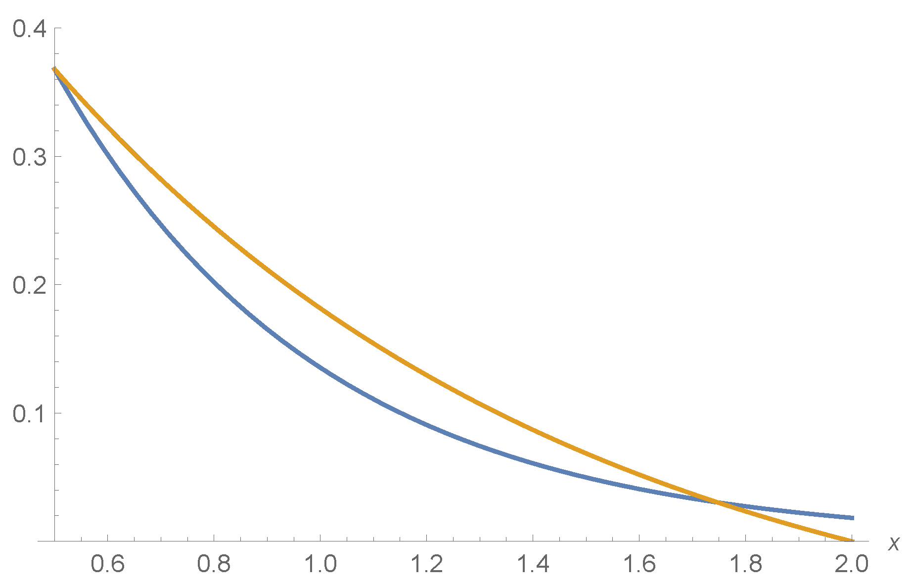
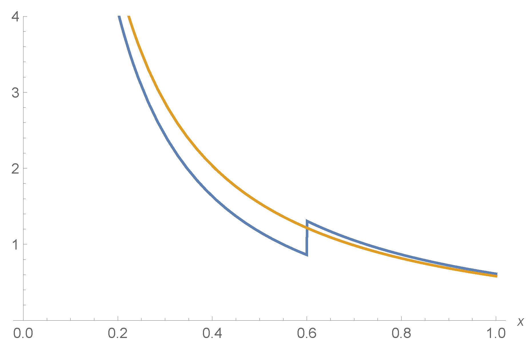
Note that, from (3), we have

$$\frac{f(x)}{f_{u,t}^{(Y)}(x)}=\left\{\begin{array}{cc}1\hfill & \mathrm{if}0\le x\le u\hfill \\ 2e^{-(x-u)}(1-e^{-(t-u)})\hfill & \mathrm{if}u<x\le t\hfill \end{array}\right.$$

(8)

and, thus, for $x\to u^{+}$ the ratio $f(x)/f_{u,t}^{(Y)}(x)$ is greater than 1 for $t-u>log2$. Hence, (ii) of Theorem 2 holds.

We have that ${\lambda }_{u,t}^{(Y)}(x)\le {\lambda }_X(x)$$\forall x>0$ is not true. Indeed, ${\lambda }_X(x)=2$ and, due to (5),

$${\lambda }_{u,t}^{(Y)}(x)=\left\{\begin{array}{cc}2\hfill & \mathrm{if}0\le x\le u\hfill \\ {\displaystyle \frac{1}{1-e^{-(t-x)}}}\hfill & \mathrm{if}u<x\le t.\hfill \end{array}\right.$$

We observe that ${\lambda }_{u,t}^{(Y)}(x)<2$ for $t-x>log2$, and that ${lim}_{x\to t^{-}}{\lambda }_{u,t}^{(Y)}(x)=\infty$. This confirms the validity of the Statement (iii) of Theorem 2.

Let us now compare stochastically the random variables X and $X_{u,t}^{(Y)}$. Due to (4), from Figure 2, we can see that

$$\overline{F}(x)\nleqq \overline{F}(u)\frac{G(t)-G(x)}{G(t)-G(u)}\forall u<x\le t.$$

Hence, (iv) of Theorem 2 holds true.

Due to (6), we have

$$r_Y(x)=\frac{e^{-x}}{1-e^{-x}},x>0,r_{u,t}^{(Y)}(x)=\left\{\begin{array}{cc}{\displaystyle \frac{2e^{-2x}}{1-e^{-2x}}}\hfill & \mathrm{if}0<x\le u\hfill \\ {\displaystyle \frac{e^{-x}{e}^{-2u}}{(1-e^{-2u})(e^{-x}-e^{-t})+e^{-u}-e^{-x}}}\hfill & \mathrm{if}u<x\le t.\hfill \end{array}\right.$$

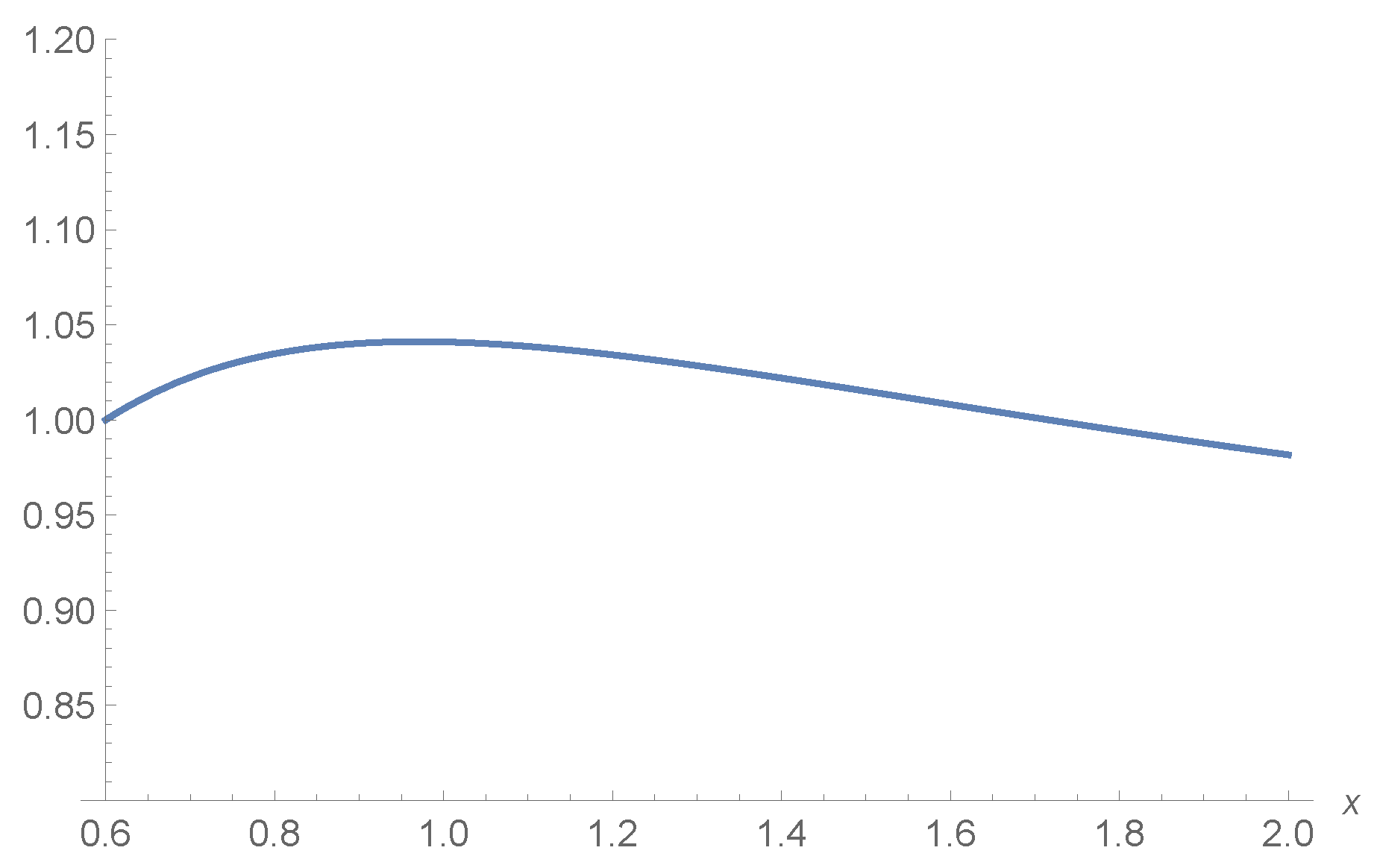
In general, such reversed hazard rates are not ordered. This can be seen in Figure 3, for instance. Hence, (v) of Theorem 2 is true.

Moreover, due to (2), we have that the ratio $F(x)/F_{u,t}^{(Y)}(x)$ is not monotone decreasing (see Figure 4), so that (vi) of Theorem 2 is fulfilled.

Let us now give another result that is based on stochastic orderings.

Theorem 3.

Let X, Y be random lifetimes. If $X{\le }_{\mathrm{st}}{X}_{u,t}^Y$$\forall u,t>0$, then $X{\le }_{\mathrm{hr}}Y$.

Proof. 

If $X{\le }_{\mathrm{st}}{X}_{u,t}^Y$ $\forall t>0$, we get

$$F(x)\ge F(u)+\frac{G(x)-G(u)}{G(t)-G(u)}\overline{F}(u),0<u<x<t.$$

(9)

From Equation (9), we get

$$\frac{F(x)-F(u)}{x-u}\frac{1}{\overline{F}(u)}\ge \frac{G(x)-G(u)}{x-u}\frac{1}{\overline{G}(u)}.$$

In the limit for $x\downarrow u$, we have ${\lambda }_X(u)\ge {\lambda }_Y(u)$ for all $u>0$ and, thus, $X{\le }_{\mathrm{hr}}Y.$ □

4. Further Comparison Results

Aiming to perform suitable comparisons, hereafter we introduce the random lifetime of the system when the replacement mechanism involves random variables having the same distribution. Specifically, we consider the case when that the random lifetimes of the two items are identically distributed, i.e., $X\stackrel{d}{=}Y$. In this case, for simplicity we denote by $X_{u,t}$, instead of $X_{u,t}^{(X)}$, the random past lifetime of the system. Hence, from Equation (1) and assumption $G(x)=F(x)$, $\forall x\in ℝ$, we have

$$X_{u,t}=\left\{\begin{array}{cc}[X|X\le u]\hfill & \mathrm{if}0\le X\le u\hfill \\ [X|u<X\le t]\hfill & \mathrm{if}X>u.\hfill \end{array}\right.$$

(10)

Clearly, in this case we implicitly assume that $\mathbb{P}(u<X\le t)>0$, i.e., $F(u)<F(t)$ for fixed $u<t$. The relevant functions concerning $X_{u,t}$, such as the distribution function $F_{u,t}(x)$, the probability density $f_{u,t}(x)$, the survival function ${\overline{F}}_{u,t}(x)$, the hazard rate ${\lambda }_{u,t}(x)$, and the reversed hazard rate $r_{u,t}(x)$ can be easily obtained from (2)–(6) by replacing $G(·)$ with $F(·)$.

For instance, due to (4), the survival function of $X_{u,t}$ is given by

$${\overline{F}}_{u,t}(x)=\left\{\begin{array}{cc}\overline{F}(x)\hfill & \mathrm{if}0\le x\le u\hfill \\ {\displaystyle \overline{F}(u)\frac{F(t)-F(x)}{F(t)-F(u)}}\hfill & \mathrm{if}u<x\le t\hfill \\ 0\hfill & \mathrm{if}x\ge t.\hfill \end{array}\right.$$

(11)

Aiming to analyze the effect of the replacement with an item having a different distribution, hereafter we stochastically compare the random lifetimes $X_{u,t}$ and $X_{u,t}^{(Y)}$.

Theorem 4.

Let X, Y be nonnegative random variables having common support. Subsequently, for $0\le u<t$, we have $X_{u,t}{\le }_{st}{X}_{u,t}^{(Y)}$ if and only if $X{\le }_{lr}Y$.

Proof. 

Recalling the survival functions (4) and (11), we have that ${\overline{F}}_{u,t}(x)\le {\overline{F}}_{u,t}^{(Y)}(x)$ is equivalent to

$$\frac{F(t)-F(x)}{F(t)-F(u)}\le \frac{G(t)-G(x)}{G(t)-G(u)},0\le u<t.$$

Hence, the thesis follows from Theorem 1.C.5 of Shaked and Shanthikumar [29]. □

With the objective of comparing the means of $X_{u,t}^{(Y)}$ and $X_{u,t}$, we now recall that the mean inactivity time of X is expressed as

$${\overline{m}}_X(u)=𝔼[X|X\le u]={\int }_0^{u}x\frac{f(x)}{F(u)}\mathrm{d}x,$$

(12)

for all $u>0$ such that $F(u)>0$. Furthermore, the doubly truncated mean of X is

$$m_X(u,t)=𝔼[X|u<X\le t]={\int }_u^{t}x\frac{f(x)}{F(t)-F(u)}\mathrm{d}x,$$

(13)

for all $0\le u<t$, such that $F(t)-F(u)>0$, and similarly for Y.

We are now able to compare the means of $X_{u,t}^{(Y)}$ and $X_{u,t}$.

Theorem 5.

Let X, Y be absolutely continuous nonnegative random variables. Subsequently, for $0\le u<t$, we have

$$\begin{array}{c}\hfill 𝔼[X_{u,t}^{(Y)}]-𝔼[X_{u,t}]=\overline{F}(u)[m_Y(u,t)-m_X(u,t)].\end{array}$$

(14)

Proof. 

Making use of Equations (3), (12) and (13), we have

$$\begin{array}{cc}\hfill 𝔼[X_{u,t}^{(Y)}]& ={\int }_0^{\infty }x{f}_{u,t}^{(Y)}(x)\mathrm{d}x\hfill \\ & ={\int }_0^{u}xf(x)\mathrm{d}x+{\int }_u^{t}x\frac{g(x)}{G(t)-G(u)}\overline{F}(u)\mathrm{d}x\hfill \\ & =F(u){\overline{m}}_X(u)+\overline{F}(u)m_Y(u,t).\hfill \end{array}$$

When X and Y are identically distributed, we clearly have

$$𝔼[X_{u,t}]=F(u){\overline{m}}_X(u)+\overline{F}(u)m_X(u,t).$$

The result (14) thus immediately follows. □

Aiming to compare the means considered in Theorem 5, we recall the following definition given in Navarro et al. [30].

Definition 2.

Let X and Y have supports $S_X$ and $S_Y$, respectively, with $S_X\cap S_Y\ne \varnothing$. Afterwards, X is said to be smaller than Y in the mean doubly truncated order ($X{\le }_{mdt}Y$) if $m_X(t_1,t_2)\le m_Y(t_1,t_2)$ for all $t_1,t_2\in S_X\cap S_Y$, with $t_1<t_2$.

We are now able to state a comparison result for the means of the system lifetime.

Proposition 1.

We have $𝔼[X_{u,t}]\le 𝔼[X_{u,t}^{(Y)}]$, for $0\le u<t$, if and only if $X{\le }_{mdt}Y$.

Proof. 

The proof follows from (14) and Definition 2. □

The following proposition is immediate from the above result and Proposition 3.3 and Theorem 3.6 of [30].

Proposition 2.

Let X and Y have common support. Subsequently, $E[X_{u,t}]\le E[X_{u,t}^{(Y)}]$, for $0\le u<t$, if and only if $X{\le }_{lr}Y$.

5. Relative Ratio of Improvement

In this section, we refer to a system having random lifetime X, which is replaced by Y at time u. Clearly, if X is smaller than Y according to some stochastic order, then it is reasonable that the reliability of the system improves at time x, for $u<x<t$, under the assumptions specified in Section 2. Aiming to measure the usefulness of the replacement, let us now introduce the relative ratio of improvement evaluated at $u<x<t$, defined in terms of (4) as

$$R_{u,t}(x):=\frac{\overline{F}(x)-{\overline{F}}_{u,t}^{(Y)}(x)}{\overline{F}(x)}=1-\frac{\overline{F}(u)}{\overline{F}(x)}\frac{G(t)-G(x)}{G(t)-G(u)},u<x<t.$$

(15)

Clearly, from (15), one has

$$\underset{x\to u^{+}}{lim}{R}_{u,t}(x)=0,\underset{x\to t^{-}}{lim}{R}_{u,t}(x)=1.$$

The measure of differential with the new variable Y is denoted with

$$R_{u,t}^{*}(x):=\frac{\overline{G}(x)-{\overline{F}}_{u,t}^{(Y)}(x)}{\overline{G}(x)}=1-\frac{\overline{F}(u)}{\overline{G}(x)}\frac{G(t)-G(x)}{G(t)-G(u)},u<x<t.$$

(16)

In this case, (16) gives

$$\underset{x\to u^{+}}{lim}{R}_{u,t}^{*}(x)=1-\frac{\overline{F}(u)}{\overline{G}(u)},\underset{x\to t^{-}}{lim}{R}_{u,t}^{*}(x)=1.$$

Theorem 6.

Let X and Y be absolutely continuous nonnegative random variables. It results that

(i) if $X{\ge }_{\mathrm{hr}}Y$, then the function $R_{u,t}(x)$ is increasing in x, for $u<x<t$;

(ii) the function $R_{u,t}^{*}(x)$ is increasing in x, for $u<x<t$.

Proof. 

From (15) and from straightforward calculations, we get

$$\frac{\mathrm{d}}{\mathrm{d}x}{R}_{u,t}(x)=\frac{\overline{F}(u)[G(t)-G(x)]}{\overline{F}(x)[G(t)-G(u)]}\left[\frac{g(x)}{\overline{G}(x)-\overline{G}(t)}-\frac{f(x)}{\overline{F}(x)}\right],u<x<t.$$

Subsequently, from hypothesis $X{\ge }_{\mathrm{hr}}Y$, we have $g(x)\overline{F}(x)-f(x)[\overline{G}(x)-\overline{G}(t)]\ge 0$ for $u<x<t$ and, thus, we obtain the result (i). Moreover, Equation (16) gives

$$\frac{\mathrm{d}}{\mathrm{d}x}{R}_{u,t}^{*}(x)=\frac{g(x)\overline{F}(u)\overline{G}(t)}{{\overline{G}}^2(x)[G(t)-G(u)]}\ge 0,u<x<t,$$

so that the result (ii) follows. □

The following example investigates $R_{u,t}(x)$ and $R_{u,t}^{*}(x)$ when X and Y are exponentially distributed.

Example 3.

Let X and Y be exponentially distributed with parameters 1 and λ, respectively. Figure 5 shows $R_{u,t}(x)$ and $R_{u,t}^{*}(x)$ for some choices of λ.

6. Results Based on Entropies

In this section, we study some informational properties of the random past lifetime $X_{u,t}^{(Y)}$. It is well known that the differential entropy of a nonnegative and absolutely continuous random variable X, with PDF f, can be expressed as

$$\begin{array}{c}\hfill H_X=-{\int }_0^{\infty }f(x)logf(x)\mathrm{d}x=-𝔼[logf(X)].\end{array}$$

(17)

Hence, the differential entropy of $[X|X\le t]$, $t>0$, also named past entropy, is defined as (see [21,31])

$$\begin{array}{c}\hfill {\overline{H}}_X(t)=-{\int }_0^t\frac{f(x)}{F(t)}log\frac{f(x)}{F(t)}\mathrm{d}x,t>0,F(t)>0.\end{array}$$

The latter identity implies that

$$\begin{array}{c}\hfill -{\int }_0^{t}f(x)logf(x)\mathrm{d}x=F(t)[{\overline{H}}_X(t)-logF(t)],t>0.\end{array}$$

(18)

We recall that the partition entropy of X evaluated at time t is given by (see, for instance, Bowden [32,33])

$$\begin{array}{c}\hfill {\mathcal{P}}_X(t)=-F(t)logF(t)-\overline{F}(t)log\overline{F}(t),t>0.\end{array}$$

(19)

The interval entropy of X in the interval $[t_1,t_2]$ is (see, for instance, Sunoj et al. [19], and Misagh and Yari [34])

$$\begin{array}{c}\hfill H_X(t_1,t_2)=-{\int }_{t_1}^{t_2}\frac{f(x)}{F(t_2)-F(t_1)}log\frac{f(x)}{F(t_2)-F(t_1)}\mathrm{d}x.\end{array}$$

(20)

The interval entropy of Y can be defined similarly. Moreover, from (20), it is not hard to see that when $t_2\to \infty$ one has

$$\begin{array}{c}\hfill \underset{t_2\to \infty }{lim}{H}_X(t_1,t_2)=-{\int }_{t_1}^{\infty }\frac{f(x)}{\overline{F}(t_1)}log\frac{f(x)}{\overline{F}(t_1)}\mathrm{d}x=:H_X(t_1),\end{array}$$

(21)

where the latter term is also known as residual entropy of X, i.e., the differential entropy of $[X-t|X>t]$ (see [31,35,36]).

We are now able to determine an expression of the differential entropy of the random past lifetime defined in (1).

Proposition 3.

The differential entropy of $X_{u,t}^{(Y)}$ is given by

$$\begin{array}{c}\hfill H_{X_{u,t}^{(Y)}}={\mathcal{P}}_X(u)+F(u){\overline{H}}_X(u)+\overline{F}(u)H_Y(u,t),0<u<t.\end{array}$$

(22)

Proof. 

Recalling Equations (3) and (17), we have that

$$\begin{array}{cc}\hfill H_{X_{u,t}^{(Y)}}& =-{\int }_0^{\infty }{f}_{u,t}^{(Y)}(x)log{f}_{u,t}^{(Y)}(x)\mathrm{d}x\hfill \\ & =-{\int }_0^{u}f(x)logf(x)\mathrm{d}x-{\int }_u^t\frac{g(x)}{G(t)-G(u)}\overline{F}(u)log\left(\frac{g(x)}{G(t)-G(u)}\overline{F}(u)\right)\mathrm{d}x\hfill \\ & =-{\int }_0^{u}f(x)logf(x)\mathrm{d}x-\overline{F}(u){\int }_u^t\frac{g(x)}{G(t)-G(u)}log\left(\frac{g(x)}{G(t)-G(u)}\right)\mathrm{d}x\hfill \\ & \hspace{1em}-\overline{F}(u)log\overline{F}(u){\int }_u^t\frac{g(x)}{G(t)-G(u)}\mathrm{d}x.\hfill \end{array}$$

Hence, by taking into account the interval entropy of Y in the interval $[u,t]$ (see, e.g., (20)), we get

$$\begin{array}{c}\hfill H_{X_{u,t}^{(Y)}}=-{\int }_0^{u}f(x)logf(x)\mathrm{d}x+\overline{F}(u)H_Y(u,t)-\overline{F}(u)log\overline{F}(u).\end{array}$$

Making use of (18) and (19), it is not hard to see that Equation (22) holds. The proof is thus completed. □

It is interesting to illustrate the meaning of Equation (22). The uncertainty about the failure time of an item distributed as the past lifetime $X_{u,t}^{(Y)}$ can be decomposed into three terms: (i) the uncertainty on whether the item has failed before or after time u (according to the distribution of X), (ii) the uncertainty about the failure time in $(0,u)$ given that the item has failed before t, and (iii) the uncertainty about the failure time in interval $(u,t)$, given that the item has failed after u and, thus, the failure time is distributed as $Y\in (u,t)$ since the replacement occurred at time u.

Remark 1.

With reference to the right-hand-side of Equation (22), we note that, using (3), (18) and (19), it is possible to obtain another form of $H_Y(u,t)$, for $0<u<t$, given by:

$$\begin{array}{cc}\hfill H_Y(u,t)& =\frac{1}{G(t)-G(u)}\hfill \\ & \times \left[G(t)\left({\overline{H}}_Y(t)-log\frac{G(t)}{G(t)-G(u)}\right)-G(u)\left({\overline{H}}_Y(u)-log\frac{G(u)}{G(t)-G(u)}\right)\right].\hfill \end{array}$$

Moreover, passing to the limit as $t\to \infty$ and recalling (21), one has

$$H_Y(u)=\underset{t\to \infty }{lim}{H}_Y(u,t)=\frac{1}{\overline{G}(u)}\left[H_Y-{\mathcal{P}}_Y(u)-G(u){\overline{H}}_Y(u)\right].$$

Hence, from Equation (22), we finally obtain:

$$\underset{t\to \infty }{lim}{H}_{X_{u,t}^{(Y)}}={\mathcal{P}}_X(u)+F(u){\overline{H}}_X(u)+\overline{F}(u)H_Y(u),u>0.$$

It is worth pointing out that the latter relation is in agreement with the result provided in Proposition 2 of [3].

If the distributions of X and Y are identical, we denote by $H_{X_{u,t}}$ the differential entropy of the past lifetime $X_{u,t}$, whose survival function has been expressed in (11). Subsequently, from Proposition 3, we have

$$\begin{array}{c}\hfill H_{X_{u,t}}={\mathcal{P}}_X(u)+F(u){\overline{H}}_X(u)+\overline{F}(u)H_X(u,t),0<u<t.\end{array}$$

(23)

Substracting (23) from (22) we get

$$\begin{array}{c}\hfill H_{X_{u,t}^{(Y)}}-H_{X_{u,t}}=\overline{F}(u)[H_Y(u,t)-H_X(u,t)],0<u<t.\end{array}$$

(24)

Here, we can introduce the following stochastic order.

Definition 3.

Let X and Y be random lifetimes; X is said to have less uncertainty in interval than Y, and write $X{\le }_{\mathrm{LUI}}Y$, if

$$H_X(u,t)\le H_Y(u,t)forall0<u<t.$$

We remark that the ${\le }_{\mathrm{LUI}}$-order is analogous to the ${\le }_{\mathrm{LU}}$-order, which was introduced by Ebrahimi ad Pellerey in [36] in order to compare the information contents in random lifetimes and to perform classification of systems. Hence, recalling the interval entropy (20), Definition 3 expresses that, given two systems that are both failed in the interval $[u,t]$, the condition $H_X(u,t)\le H_Y(u,t)$ expresses that the uncertainty about the predictability of the failure time occurred in the interval $[u,t]$ for the first system is less than that for the second one in the same interval.

Thus, we have the following result, which is similar to Corollary 1 of [3].

Proposition 4.

Let $0<u<t$. We have $H_{X_{u,t}}\le H_{X_{u,t}^{(Y)}}$ if and only if $X{\le }_{\mathrm{LUI}}Y$.

Proof. 

The result follows from (24) and from Definition 3. □

We remark that the differential entropy of $X_{u,t}^{(Y)}$ is dependent on t through the interval entropy of Y. Namely, from (22) one has that $H_{X_{u,t}^{(Y)}}$ is increasing (decreasing) in $t>u$ if and only if $H_Y(u,t)$ is increasing (decreasing) in $t>u$, for fixed $u>0$. Although the monotonicity of $H_Y(u,t)$ is relevant to establish that it uniquely determines the underlying distribution function (see Proposition 2.1 of [34]), it is not easy to establish conditions leading to its validity. This can be seen, for instance, by exploiting the conditions stated in Equations (2.9) and (2.10) of [19].

We conclude this section by analyzing the informational properties for the considered replacement model when the involved distributions arise as a special case of the generalized extreme value distribution.

Example 4.

We suppose that X and Y have Fréchet distribution, with

$$F(t)=e^{-{(t/\lambda )}^{-\alpha }},G(t)=e^{-{(t/\mu )}^{-\beta }},t>0,$$

for $\lambda ,\alpha ,\mu ,\beta >0$. It is not hard to see that these distributions have decreasing reversed hazard rate functions. From Equation (17), we can determine the differential entropy of X, given by

$$H_X=1+\frac{\gamma }{\alpha }(1+\alpha )+log\left(\frac{\lambda }{\alpha }\right),$$

where $\gamma \simeq 0.577216$ is the Euler–Mascheroni constant. We recall that such a constant can be represented in the integral form $\gamma =-{\int }_0^{\infty }{e}^{-x}logx\mathrm{d}x$. The past entropy of X can be determined by making use of (18), and taking into account that, for $t>0$,

$$\begin{array}{cc}\hfill -{\int }_0^{t}f(x)logf(x)\mathrm{d}x& =\frac{1}{\alpha }{e}^{-{(\lambda /t)}^{\alpha }}\left[(1+\alpha )e^{{(\lambda /t)}^{\alpha }}\mathrm{Ei}\left(-{\left(\frac{\lambda }{t}\right)}^{\alpha }\right)\right.\hfill \\ & -\left.\alpha \left(-1-{\left(\frac{\lambda }{t}\right)}^{\alpha }+log\alpha +\alpha log\lambda -(1+\alpha )logt\right)\right],\hfill \end{array}$$

where $Ei(z)=-{\int }_{-z}^{\infty }(e^{-t}/t)\mathrm{d}t$ is the exponential integral function. Hence, one has

$$\begin{array}{cc}\hfill {\overline{H}}_X(t)& =-{\left(\frac{t}{\lambda }\right)}^{-\alpha }+\frac{1}{\alpha }\left[(1+\alpha )e^{{(\lambda /t)}^{\alpha }}\mathrm{Ei}\left(-{\left(\frac{\lambda }{t}\right)}^{\alpha }\right)\right.\hfill \\ & -\left.\alpha \left(-1-{\left(\frac{\lambda }{t}\right)}^{\alpha }+log\alpha +\alpha log\lambda -(1+\alpha )logt\right)\right],t>0.\hfill \end{array}$$

From (20), we also obtain the interval entropy of Y in the interval $[u,t]$:

$$\begin{array}{cc}\hfill H_Y(u,t)& =-{\int }_u^t\frac{g(x)}{G(t)-G(u)}log\frac{g(x)}{G(t)-G(u)}\mathrm{d}x\hfill \\ & =\frac{{(ut)}^{-\beta }}{\beta \left(e^{{(u/\mu )}^{-\beta }}-e^{{(t/\mu )}^{-\beta }}\right)}\{\beta \left(e^{{(t/\mu )}^{-\beta }}{(\mu u)}^{\beta }-e^{{(u/\mu )}^{-\beta }}{(\mu t)}^{\beta }\right)\hfill \\ & +{(ut)}^{\beta }\left[e^{{(t/\mu )}^{-\beta }}\right(-(1+\beta )e^{{(u/\mu )}^{-\beta }}\left[\mathrm{Ei}\left(-{\left(\frac{u}{\mu }\right)}^{-\beta }\right)-\mathrm{Ei}\left(-{\left(\frac{t}{\mu }\right)}^{-\beta }\right)\right]\hfill \\ & +\beta \left[-1-log\left(\frac{1}{\beta }\left(e^{{(u/\mu )}^{-\beta }}-e^{{(t/\mu )}^{-\beta }}\right)\right)+\beta log\mu -(1+\beta )logu\right])\hfill \\ & -\beta e^{{(u/\mu )}^{-\beta }}\left[-1-log\left(\frac{1}{\beta }\left(e^{{(u/\mu )}^{-\beta }}-e^{{(t/\mu )}^{-\beta }}\right)\right)+\beta log\mu -(1+\beta )logt\right]\left]\right\}.\hfill \end{array}$$

Clearly, the partition entropy of X immediately follows from (19). Hence, by combining the above quantities, from Equation (22) we can determine the differential entropy of $X_{u,t}^{(Y)}$. We omit the expression for brevity. Nevertheless, in Figure 6, we provide some plots of $H_{X_{u,t}^{(Y)}}$, obtained by means of Proposition 3 and resorting to numerical evaluations. In all cases, we take $u=1$, and the differential entropy of $X_{u,t}^{(Y)}$ is increasing in $t>1$ and approaches a finite limit as $t\to \infty$. Hence, the information amount about the replacement at time u is increasing in the inspection time t, if at time t the considered system is found to be failed. From the given plots, we note that the entropy under investigation is not always monotone in the given parameters for fixed values of t.

We point out that the distributions considered in Example 4 satisfy the proportional reversed hazard rate property. Indeed, distributions satisfying this property are often used in stochastic models that involve the past lifetime and the past entropy (see, for instance, Nanda and Das [37]), because the proportionality condition of the reversed hazard rates leads to more manageable results.

7. Application to a Stochastic Neuronal Model

The stochastic model considered in this paper can also be used in other applied contexts, in which the replacement occurring at time u can be viewed as a relevant changing point, i.e., an event that produces a variation in the dynamics of the system under investigation. A typical case of interest in theoretical neurobiology concerns the activity of a single neuron, which is slowed during a refractory period. Specific assumptions are used to suitably describe such a refractory period within neuronal models. For instance, the modification of the upper (time-varying) firing threshold is often employed. In this context, the replacement model that is presented in Section 2 is useful to describe a modification in the neuronal dynamics occurring at time u, which can be viewed as the final instant of the refractory period. Now, we take as a reference a stochastic model for the firing activity of a neuronal unit that has been investigated by Di Crescenzo and Martinucci [38] and D’Onofrio et al. [39]. It includes the decay effect of the membrane potential in absence of stimuli, and the occurrence of Poisson-paced excitatory inputs modeled by jumps of random amplitudes. Specifically, we assume that the neuronal membrane potential at time t is denoted by

$$V(t)=v_{0}exp\left\{-\tau t+\sum _{k=1}^{N(t)}{Z}_k\right\},t>0,V(0)=v_0,$$

where

-

$v_0$ is the level of the membrane potential at initial time, just after a spike occurrence;

-

$\tau >0$ is a parameter that describes how fast the membrane potential exponentially decays to the resting level in absence of stimuli;

-

$N(t)$, $t\ge 0$, is a Poisson process with intensity $\lambda >0$ that describes the number of excitatory pulses received by the neuron in $(0,t]$; and,

-

${(Z_k)}_{k\in \mathbb{N}}$ is a sequence of i.i.d. exponentially distributed random variables with mean ${\alpha }^{-1}>0$, which are independent on $N(t)$. For fixed value of the membrane potential before the occurrence of the n-th excitatory stimulus, the mean amplitude of the n-th jump is inversely proportional to $\alpha$, so that large values of $\alpha$ reduce the effect of the neuronal excitatory activity.

For such a model, the probability density of the firing time is obtained in closed form for $\beta >v_0$ and it is given by (cf. Theorem 3.1 of [38])

$$\begin{array}{cc}\hfill h(t;\lambda ,\alpha )& =\frac{\lambda \tau t}{log\frac{\beta }{v_0}+\tau t}exp\{-(\lambda +\alpha \tau )t\}{\left(\frac{\beta }{v_0}\right)}^{-\alpha }\hfill \\ & \times \left\{\frac{I_1\left(2\sqrt{\lambda \alpha t(log\frac{\beta }{v_0}+\tau t)}\right)}{\sqrt{\lambda \alpha t(log\frac{\beta }{v_0}+\tau t)}}+\left(log\frac{\beta }{v_0}\right)\frac{I_0\left(2\sqrt{\lambda \alpha t(log\frac{\beta }{v_0}+\tau t)}\right)}{\tau t}\right\},t>0\hfill \end{array}$$

(25)

where

$$I_n(x)=\sum _{k=0}^{+\infty }\frac{{(x/2)}^{n+2k}}{k!(n+k)!},n\in {\mathbb{N}}_0$$

is modified Bessel function of the first kind. We note that

$$\underset{t\to 0}{lim}h(t;\lambda ,\alpha )=\lambda {\left(\frac{\beta }{v_0}\right)}^{-\alpha }.$$

With reference to the replacement model considered above, we assume that the random variables X and Y possess PDF’s given by

$$f(t)=h(t;{\lambda }_1,{\alpha }_1),g(t)=h(t;{\lambda }_2,{\alpha }_2),t>0,$$

(26)

with $0<{\lambda }_1<{\lambda }_2$ and $0<{\alpha }_2<{\alpha }_1$, and where h corresponding to the firing PDF given in (25). The assumptions given on the parameters ${\lambda }_i,{\alpha }_i$, $i=1,2$, imply that after the replacement time u, the neuronal unit undergoes different dynamics producing more frequent excitatory pulses, having greater and greater strength. Hence, it is expected that the performed modification produces an increment of the relevant rates of the stochastic system under investigation.

For a suitable illustration, we consider the following choices of the involved parameters suggested by various investigations dealing with reasonably physiologic values (see [38] and references therein): $\tau =0.2$ ms${}^{-1}$, $\beta =20$ mV, $v_0=10$ mV, ${\lambda }_1=2$ ms${}^{-1}$, ${\lambda }_2=2.2$ ms${}^{-1}$, ${\alpha }_1=6$ mV${}^{-1}$, and ${\alpha }_2=5$ mV${}^{-1}$. Figure 7 shows the effect of the replacement on the hazard rate (5) and on the reversed hazard rate (6), confirming that the replacement produces an increment of such rates.

8. Conclusions

The determination of a policy for the replacement or the improvement of the components of a system is a relevant problem in Engineering Reliability. In this framework, several criteria have been proposed and analyzed in the literature in the recent years. The availability of the system is improved often by means of replacements or duplications of the involved subsystems. Large attention has been devoted to the reliability analysis based on information on the past history of the system. Less attention has been devoted to the cases when the uncertainty is related to the previous status of the system. Within such framework, in this paper we continued the study of a replacement model considered in [3]. In the previous paper, the replacement is planned in advance, the replaced item possessing a different failure distribution and having the same age of the replaced item. Here, the new results are obtained assuming that the replacement of the first item by the second one (having the same age) is planned to occur at time u, provided that the first item has not failed before. Moreover, we assume that the system is interrupted at the inspection time $t>u.$

The investigation has been centered on the stochastic comparison of the resulting random lifetimes. We also performed suitable stochastic comparisons between the system past lifetime and the lifetimes of the single items. Furthermore, the goodness of the replacement criteria has been studied by means of the relative ratio of improvement. The dynamic information concerning by the system lifetime has been analyzed using the differential entropy. An application to a stochastic neuronal model has also been provided.

Possible future developments on this model can be finalized to the extension to multidimensional instances in which several replacement are planned at subsequent times in order to improve the reliability of the system.