Q-Curve and Area Rules for Choosing Heuristic Parameter in Tikhonov Regularization

Abstract

We consider choice of the regularization parameter in Tikhonov method if the noise level of the data is unknown. One of the best rules for the heuristic parameter choice is the quasi-optimality criterion where the parameter is chosen as the global minimizer of the quasi-optimality function. In some problems this rule fails. We prove that one of the local minimizers of the quasi-optimality function is always a good regularization parameter. For the choice of the proper local minimizer we propose to construct the Q-curve which is the analogue of the L-curve, but on the x-axis we use modified discrepancy instead of discrepancy and on the y-axis the quasi-optimality function instead of the norm of the approximate solution. In the area rule we choose for the regularization parameter such local minimizer of the quasi-optimality function for which the area of the polygon, connecting on Q-curve this minimum point with certain maximum points, is maximal. We also provide a posteriori error estimates of the approximate solution, which allows to check the reliability of the parameter chosen heuristically. Numerical experiments on an extensive set of test problems confirm that the proposed rules give much better results than previous heuristic rules. Results of proposed rules are comparable with results of the discrepancy principle and the monotone error rule, if the last two rules use the exact noise level.

1. Introduction

Let $A\in \mathcal{L}(H,F)$ be a linear bounded operator between real Hilbert spaces H, F. We are interested in finding the minimum norm solution $u_{*}$ of the equation

$$Au=f_{*},f_{*}\in \mathcal{R}(A),$$

(1)

where noisy data $f\in F$ are given instead of the exact data $f_{*}$. The range $\mathcal{R}(A)$ may be non-closed and the kernel $\mathcal{N}(A)$ may be non-trivial, so in general this problem is ill-posed. We consider the solution of the problem $Au=f$ by the Tikhonov method (see [1,2]) where the regularized solutions in cases of exact and inexact data have the corresponding forms

$$u_{\alpha }^{+}={\left(\alpha I+A^{*}A\right)}^{-1}{A}^{*}{f}_{*},u_{\alpha }={\left(\alpha I+A^{*}A\right)}^{-1}{A}^{*}f$$

and $\alpha >0$ is the regularization parameter. Using the well-known estimate $∥u_{\alpha }-u_{\alpha }^{+}∥\le \frac{1}{2}{\alpha }^{-1/2}∥f-f_{*}∥$ (see [1,2]) and notations

$$e(\alpha ):=∥u_{\alpha }-u_{*}∥,e_1(\alpha ):=∥u_{\alpha }^{+}-u_{*}∥+∥u_{\alpha }-u_{\alpha }^{+}∥,$$

(2)

$$e_2(\alpha ,∥f-f_{*}∥):=∥u_{\alpha }^{+}-u_{*}∥+\frac{1}{2\sqrt{\alpha }}∥f-f_{*}∥,$$

we have the error estimates

$$e(\alpha )\le e_1(\alpha )\le e_2(\alpha ,∥f-f_{*}∥).$$

(3)

We consider choice of the regularization parameter if the noise level for $∥f-f_{*}∥$ is unknown. The parameter choice rules which do not use the noise level information are called heuristic rules. Well known heuristic rules are the quasi-optimality criterion [3,4,5,6,7,8,9], L-curve rule [10,11], GCV (generalized cross-validation)-rule [12], Hanke–Raus rule [13], Reginska’s rule [14] and its modifications [15]; for other rules see [16,17,18]. Heuristic rules are numerically compared in [4,17,18,19]. The heuristic rules give good results in many problems, but it is not possible to construct heuristic rules guaranteeing convergence $∥u_{\alpha }-u_{*}∥\to 0$ as the noise level goes to zero (see [20]). All heuristic rules may fail in some problems and without additional information about the solution, it is difficult to decide, is the obtained parameter reliable or not.

In the quasi-optimality criterion the parameter $\alpha$ is chosen as the global minimizer of the function ${\psi }_{\mathrm{Q}}(\alpha )=\alpha ∥\frac{d{u}_{\alpha }}{d\alpha }∥$ on certain interval. We propose to choose the parameter from the set $L_{\min }$ of local minimizers of this function from certain set $\Omega$ of parameters.

We will call the parameter ${\alpha }_{\mathrm{R}}$ in arbitrary rule R as pseudooptimal, if

$$∥u_{{\alpha }_{\mathrm{R}}}-u_{*}∥\le c\underset{\alpha >0}{min}{e}_1(\alpha )$$

with relatively small constant c and we show that at least one parameter from set $L_{\min }$ has this property. For the choice of proper parameter from the set $L_{\min }$ some algorithms were proposed in [21], in the current work we propose other algorithms. We propose to construct the Q-curve which is the analogue of the L-curve [10], but on the x-axis we use modified discrepancy instead of discrepancy and on the y-axis function ${\psi }_{\mathrm{Q}}(\alpha )$ instead of $\parallel u_{\alpha }\parallel .$ For finding proper local minimizer of the function ${\psi }_{\mathrm{Q}}(\alpha )$, we propose the area rules on the Q-curve. The idea of proposed rules is that we form, for every minimizer of the function ${\psi }_{\mathrm{Q}}(\alpha )$, a certain function which approximates the error of the approximate solution and has one minimizer; we choose for the regularization parameter such local minimizer of ${\psi }_{\mathrm{Q}}(\alpha )$, for which the area of the polygon, connecting this minimum point with certain maximum points, is maximal.

The plan of this paper is as follows. In Section 2 we consider known rules for choice of the regularization parameter, both in case of known and unknown noise level. In Section 3, we prove that the set $L_{\min }$ contains at least one pseudooptimal parameter. In Section 4, information about used test problems (mainly from [11,22], but also from [11,23,24,25,26]) and numerical experiments is given. In Section 5, we consider the Q-curve and area rule, in Section 6 further developments of the area rule. These algorithms are also illustrated by the results of numerical experiments.

2. Rules for the Choice of the Regularization Parameter

2.1. Parameter Choice in the Case of Known Noise Level

In the case of known noise level $\delta ,∥f-f_{*}∥\le \delta$ we use one of the so-called $\delta$-rules, where certain functional $d(\alpha )$ and constant $b\ge b_0$ ($b_0$ depends on $d(\alpha )$) are chosen and such regularization parameter $\alpha (\delta )$ is chosen which satisfies $d(\alpha )=b\delta .$

(1) Discrepancy principle (DP) [2,27]:

$$d_{\mathrm{D}}(\alpha ):=∥A{u}_{\alpha }-f∥=b\delta ,b\ge 1.$$

(2) Modified discrepancy principle (Raus–Gfrerer rule) [28,29]:

$$d_{\mathrm{MD}}(\alpha ):=∥B_{\alpha }\left(A{u}_{\alpha }-f\right)∥=b\delta ,B_{\alpha }:={\alpha }^{1/2}{\left(\alpha I+A{A}^{*}\right)}^{-1/2},b\ge 1.$$

(3) Monotone error rule (ME-rule) [30,31]:

$$d_{\mathrm{ME}}(\alpha ):=\frac{{∥B_{\alpha }\left(A{u}_{\alpha }-f\right)∥}^2}{∥B_{\alpha }^2\left(A{u}_{\alpha }-f\right)∥}=\delta .$$

The name of this rule is justified by the fact that the chosen parameter ${\alpha }_{\mathrm{ME}}$ satisfies

$$\frac{\mathrm{d}}{\mathrm{d}\alpha }\parallel u_{\alpha }-u_{*}\parallel >0\forall \alpha >{\alpha }_{\mathrm{ME}}.$$

Therefore ${\alpha }_{\mathrm{ME}}\ge {\alpha }_{\mathrm{opt}}:=\mathrm{argmin}\parallel u_{\alpha }-u_{*}\parallel$.

(4) Monotone error rule with post-estimation (MEe-rule) [4,18,32,33,34,35]. The inequality ${\alpha }_{\mathrm{ME}}\ge {\alpha }_{\mathrm{opt}}$ suggests to use somewhat smaller parameter than ${\alpha }_{\mathrm{ME}}$. Extensive numerical experiments suggest to compute ${\alpha }_{\mathrm{ME}}$ and to use the post-estimated parameter ${\alpha }_{\mathrm{MEe}}:=0.4{\alpha }_{\mathrm{ME}}$. Then typically $\parallel u_{{\alpha }_{\mathrm{MEe}}}-u_{*}\parallel /\parallel u_{{\alpha }_{\mathrm{ME}}}-u_{*}\parallel \in (0.7,0.9)$. If the exact noise level is known, this MEe-rule gives typically the best results from all $\delta$-rules.

(5) Rule R1 [36]. Let $b>\frac{2}{3\sqrt{3}}$. Choose $\alpha (\delta )$ as the smallest solution of the equation

$$d_{\mathrm{R}1}(\alpha (\delta )):={\alpha }^{-1/2}∥A^{*}{B}_{\alpha }^2\left(A{u}_{\alpha }-f\right)∥=b\delta .$$

Note that this equation can be rewritten using the 2-iterated Tikhonov approximation $u_{2,\alpha }$:

$$B_{\alpha }^2\left(A{u}_{\alpha }-f\right)=A{u}_{2,\alpha }-f,u_{2,\alpha }={\left(\alpha I+A^{*}A\right)}^{-1}(\alpha u_{\alpha }+A^{*}f).$$

(4)

The last four rules are weakly quasioptimal rules (see [37]) for the Tikhonov method: if $∥f-f_{*}∥\le \delta$, then $∥u_{\alpha (\delta )}-u_{*}∥\le C(b){inf}_{\alpha >0}{e}_2(\alpha ,\delta )$ (see (3)). The rules for the parameter choice in case of approximately given noise level are proposed and analyzed in [18,32,33,34].

2.2. Parameter Choice in the Case of Unknown Noise Level

A classical heuristic rule is the quasi-optimality criterion. In the Tikhonov method, it chooses $\alpha ={\alpha }_{\mathrm{Q}}$ or $\alpha ={\alpha }_{\mathrm{QD}}$ as the global minimizer of corresponding functions

$${\psi }_{\mathrm{Q}}(\alpha )=\alpha ∥\frac{d{u}_{\alpha }}{d\alpha }∥={\alpha }^{-1}∥A^{*}{B}_{\alpha }^2\left(A{u}_{\alpha }-f\right)∥=\alpha \parallel A^{*}{\left(\alpha I+A{A}^{*}\right)}^{-2}f\parallel =\parallel u_{2,\alpha }-u_{\alpha }\parallel ,$$

(5)

$${\psi }_{\mathrm{QD}}(\alpha )={\left(1-q\right)}^{-1}∥u_{\alpha }-u_{q\alpha }∥,0<q<1.$$

(6)

The Hanke–Raus rule finds parameter $\alpha ={\alpha }_{HR}$ as the global minimizer of the function

$${\psi }_{\mathrm{HR}}(\alpha )={\alpha }^{-1/2}∥B_{\alpha }\left(A{u}_{\alpha }-f\right)∥.$$

In practice, often the L-curve is used. The L-curve is the log-log-plot of $∥u_{\alpha }∥$ versus $∥A{u}_{\alpha }-f∥$. The points $\left(∥A{u}_{\alpha }-f∥,∥u_{\alpha }∥\right)$ have often a shape similar to the letter L and the parameter ${\alpha }_L$ which corresponds to the corner point is often a good parameter. In the literature several concrete rules for choice of the corner point are proposed. In [14], a parameter is chosen as the global minimizer of the function

$${\psi }_{\mathrm{RE}}(\alpha )=∥A{u}_{\alpha }-f∥{∥u_{\alpha }∥}^{\tau },\tau \ge 1$$

(below we use this rule with $\tau =1$). Another rule for choice of the corner point is the maximum curvature method ([38,39]), where such parameter $\alpha$ is chosen for which the curvature of the L-curve as the function

$${\psi }_{\mathrm{MC}}(\alpha )=2\frac{{\widehat{\rho }}^{\prime }{\widehat{\xi }}^{″}-{\widehat{\rho }}^{″}{\widehat{\xi }}^{\prime }}{{({({\widehat{\rho }}^{\prime })}^2+{({\widehat{\xi }}^{\prime })}^2)}^{3/2}}$$

is maximal. Here ${\widehat{\rho }}^{\prime },{\widehat{\xi }}^{\prime },{\widehat{\rho }}^{″},{\widehat{\xi }}^{″}$ are first and second order derivatives of functions $log{d}_{\mathrm{D}}(\alpha )$ and $log∥u_{\alpha }∥$.

We propose also a new heuristic rule, where the global minimizer of the function

$${\psi }_{\mathrm{WQ}}(\alpha )=d_{\mathrm{MD}}(\alpha ){\psi }_{\mathrm{Q}}(\alpha )$$

(7)

is chosen for the parameter. We call this rule as the weighted quasioptimality criterion.

In the following we will find the regularization parameter from the set of parameters

$$\Omega =\left\{{\alpha }_j:{\alpha }_j=q{\alpha }_{j-1},j=1,2,\dots ,N,0<q<1\right\},$$

(8)

where ${\alpha }_0,q,{\alpha }_N$ are given. If in the discretized problem the minimal eigenvalue ${\lambda }_{\min }$ of the matrix $A^{T}A$ is larger than ${\alpha }_N$, the heuristic rules above often choose parameter ${\alpha }_N$, which is generally not a good parameter. The works [6,7,8] propose to search the global minimum of the function ${\psi }_{\mathrm{Q}}(\alpha )$ in the interval $[max\left({\alpha }_N,{\lambda }_{\min }\right),{\alpha }_0]$.

Definition 1.

We say that the discretized problem $Au=f$ does not need regularization if

$$e_1({\lambda }_{\min })\le 2\underset{\alpha \in \Omega ,\alpha \ge {\lambda }_{\min }}{min}{e}_1(\alpha ).$$

If the discretized problem does not need regularization then ${\alpha }^{\prime }=0$ or ${\alpha }^{\prime }={\alpha }_N$ is the proper parameter while for ${\alpha }^{\prime }\le {\lambda }_{min}$ we have

$$\begin{array}{c}\hfill ∥u_{{\alpha }^{\prime }}-u_{*}∥\le e_1({\alpha }^{\prime })=∥u_{{\alpha }^{\prime }}^{+}-u_{*}∥+∥{({\alpha }^{\prime }I+A^{*}A)}^{-1}{A}^{*}(f-f_{*})∥\le \\ \hfill ∥u_{{\lambda }_{min}}^{+}-u_{*}∥+2∥{({\lambda }_{min}I+A^{*}A)}^{-1}{A}^{*}(f-f_{*})∥\le 2e_1({\lambda }_{min})\le 4\underset{\alpha \in \Omega ,\alpha \ge {\lambda }_{min}}{min}{e}_1(\alpha ).\end{array}$$

Searching the parameter from the interval $[max\left({\alpha }_N,{\lambda }_{\min }\right),{\alpha }_0]$ means the a priori assumption that the discretized problem needs regularization. Note that if ${\lambda }_{\min }>{\alpha }_N$, then in general it is not possible to decide (without additional information about solution or about noise of the data) whether the discretized problem needs regularization or not.

3. Local Minimum Points of the Function ${\mathbf{\psi }}_{\mathrm{Q}}(\mathbf{\alpha })$

In the following we investigate the function ${\psi }_{\mathrm{Q}}(\alpha )$ in (5) and show that at least one local minimizer of this function is the pseudooptimal parameter. We need some preliminary results.

Lemma 1.

The functions ${\psi }_{\mathrm{Q}}(\alpha )$, ${\psi }_{\mathrm{QD}}(\alpha )$ satisfy for each $\alpha >0$ the estimates

$${\psi }_{\mathrm{Q}}(\alpha )\le e_1(\alpha ),$$

(9)

$${\psi }_{\mathrm{QD}}(\alpha )\le q^{-1}{e}_1(\alpha ),$$

(10)

$${\psi }_{\mathrm{Q}}(\alpha )\le {\psi }_{\mathrm{QD}}(\alpha )\le q^{-1}{\psi }_{\mathrm{Q}}(q\alpha ).$$

Proof. 

Using relations $f=A{u}_{*}+f-f_{*}$,

$$u_{\alpha }-u_{q\alpha }=\left(q-1\right)\alpha {\left(\alpha I+A^{*}A\right)}^{-1}{\left(q\alpha I+A^{*}A\right)}^{-1}{A}^{*}f,$$

$$∥A^{*}A{\left(\alpha I+A^{*}A\right)}^{-1}∥\le 1,\alpha ∥{\left(\alpha I+A^{*}A\right)}^{-1}∥\le 1,$$

we have

$$\begin{array}{ccc}\hfill {\psi }_{\mathrm{Q}}(\alpha )& =& \alpha \parallel A^{*}{\left(\alpha I+A{A}^{*}\right)}^{-2}f\parallel =\alpha \parallel {(\alpha I+A^{*}A)}^{-2}{A}^{*}f\parallel \hfill \\ & \le & \alpha ∥A^{*}A{\left(\alpha I+A^{*}A\right)}^{-2}{u}_{*}∥+\alpha ∥{\left(\alpha I+A^{*}A\right)}^{-2}{A}^{*}(f-f_{*})∥\hfill \\ & \le & \alpha \parallel {(\alpha I+A^{*}A)}^{-1}{u}_{*}\parallel +\parallel {(\alpha I+A^{*}A)}^{-1}{A}^{*}(f-f_{*})\parallel =e_1(\alpha ),\hfill \\ \hfill {\psi }_{\mathrm{QD}}(\alpha )& \le & \alpha ∥A^{*}A{(q\alpha I+A^{*}A)}^{-1}){(\alpha I+A^{*}A)}^{-1})u_{*}∥\hfill \\ & & +\alpha ∥{(q\alpha I+A^{*}A)}^{-1}){(\alpha I+A^{*}A)}^{-1})A^{*}(f-f_{*})∥\le q^{-1}{e}_1(\alpha ),\hfill \\ \hfill {\psi }_{\mathrm{Q}}(\alpha )& =& \alpha ∥{\left(\alpha I+A^{*}A\right)}^{-2}{A}^{*}f∥\le \alpha ∥{\left(\alpha I+A^{*}A\right)}^{-1}{\left(q\alpha I+A^{*}A\right)}^{-1}{A}^{*}f∥\hfill \\ & =& {\psi }_{\mathrm{QD}}(\alpha )\le \alpha ∥{\left(q\alpha I+A^{*}A\right)}^{-2}{A}^{*}f∥=q^{-1}{\psi }_{\mathrm{Q}}(q\alpha ).\hfill \end{array}$$

 ☐

Remark 1.

Note that ${lim}_{\alpha \to \infty }{\psi }_{\mathrm{Q}}(\alpha )=0$, but ${lim}_{\alpha \to \infty }{e}_1(\alpha )=∥u_{*}∥$. Therefore in the case of too large ${\alpha }_0$ this ${\alpha }_0$ may be a global (or local) minimizer of the function ${\psi }_{\mathrm{Q}}(\alpha )$. The scaling argument suggests: by multiplying the equation $A^{*}Au=A^{*}f$ by some constant, it is also necessary to multiply α by this constant in the Tikhonov method. Therefore the parameter ${\alpha }_0$ should be proportional to $\parallel A^{*}A\parallel$. We recommend to take ${\alpha }_0=c∥A^{*}A∥,c\le 1$ or to minimize the function ${\overline{\psi }}_{\mathrm{Q}}(\alpha ):=(1+\alpha /∥A^{*}A∥){\psi }_{\mathrm{Q}}(\alpha )$ instead of ${\psi }_{\mathrm{Q}}(\alpha )$. Due to the equality ${lim}_{\alpha \to 0}(1+\alpha /∥A^{*}A∥)=1$, the function ${\overline{\psi }}_{\mathrm{Q}}(\alpha )$ approximately satisfies (9) for small α.

In the following we define the local minimum points of the function ${\psi }_{\mathrm{Q}}(\alpha )$ on the set $\Omega$ (see (8)).

Definition 2.

We say that the parameter ${\alpha }_k,0\le k\le N-1$ is the local minimum point of the sequence ${\psi }_{\mathrm{Q}}({\alpha }_k)$, if ${\psi }_{\mathrm{Q}}({\alpha }_k)<{\psi }_{\mathrm{Q}}({\alpha }_{k+1})$ and in case $k>0$ there exists index $j\ge 1$ such that ${\psi }_{\mathrm{Q}}({\alpha }_k)={\psi }_{\mathrm{Q}}({\alpha }_{k-1})=\dots ={\psi }_{\mathrm{Q}}({\alpha }_{k-j+1})<{\psi }_{\mathrm{Q}}({\alpha }_{k-j})$. The parameter ${\alpha }_N$ is the local minimum point if there exists index $j\ge 1$ so that

$${\psi }_{\mathrm{Q}}({\alpha }_N)={\psi }_{\mathrm{Q}}({\alpha }_{N-1})=\dots ={\psi }_{\mathrm{Q}}({\alpha }_{N-j+1})<{\psi }_{\mathrm{Q}}({\alpha }_{N-j}).$$

Denote the local minimum points by $m_k$, $k=1,\dots ,K$ (K is the number of minimum points) and corresponding set by $L_{\min }=\left\{m_k:m_1>m_2>\dots >m_K\right\}.$

Definition 3.

The parameter ${\alpha }_k,0<k<N$ is the local maximum point of the sequence ${\psi }_{\mathrm{Q}}({\alpha }_k)$ if ${\psi }_{\mathrm{Q}}({\alpha }_k)>{\psi }_{\mathrm{Q}}({\alpha }_{k+1})$ and there exists index $j\ge 1$ so that

$${\psi }_{\mathrm{Q}}({\alpha }_k)={\psi }_{\mathrm{Q}}({\alpha }_{k-1})=\dots ={\psi }_{\mathrm{Q}}({\alpha }_{k-j+1})>{\psi }_{\mathrm{Q}}({\alpha }_{k-j}).$$

We denote by $M_k$ the local maximum point between the local minimum points $m_{k+1}$ and $m_k,1\le k\le K-1$. Denote $M_0={\alpha }_0$, $M_K={\alpha }_N$. Then by the construction

$$M_K\le m_K<M_{K-1}<\dots <m_2<M_1<m_1\le M_0.$$

Theorem 1.

The following estimates hold for the local minimizers of the function ${\psi }_{\mathrm{Q}}(\alpha )$.

1 

For arbitrary ${\alpha }_0,{\alpha }_N$ we have

$$\underset{\alpha \in L_{\min }}{min}∥u_{\alpha }-u_{*}∥\le q^{-1}C\underset{{\alpha }_N\le \alpha \le {\alpha }_0}{min}{e}_1(\alpha ),$$

(11)

$$C:=1+\underset{1\le k\le K}{max}\underset{{\alpha }_j\in \Omega ,M_k\le {\alpha }_j\le M_{k-1}}{max}T\left(m_k,{\alpha }_j\right)\le 1+c_{q}ln\left(\frac{{\alpha }_0}{{\alpha }_N}\right),T(\alpha ,\beta ):=\frac{∥u_{\alpha }-u_{\beta }∥}{{\psi }_{\mathrm{Q}}(\beta )}.$$

2 

If ${\alpha }_0=∥A^{*}A∥$, ${\alpha }_N={\alpha }_0{\left(\frac{∥f-f_{*}∥}{2∥u_{*}∥}\right)}^2$, then

$$\underset{\alpha \in L_{\min }}{min}∥u_{\alpha }-u_{*}∥\le q^{-1}(1+2max\{1,c_q\mid ln\frac{∥f-f_{*}∥}{2∥A∥∥u_{*}∥}\mid \})\underset{\alpha >0}{min}{e}_2(\alpha ,∥f-f_{*}∥),$$

(12)

where $c_q:=\left(q^{-1}-1\right)/ln{q}^{-1}\to 1 if q\to 1$.

Moreover, if $u_{*}={\left|A\right|}^{p}v$, $∥v∥\le \rho$, $p>0$, where $\left|A\right|:={(A^{*}A)}^{1/2}$, then

$$\underset{\alpha \in L_{\min }}{min}∥u_{\alpha }-u_{*}∥\le c_{p,q}{\rho }^{\frac{1}{p+1}}\left|ln∥f-f_{*}∥\right|{∥f-f_{*}∥}^{\frac{p}{p+1}},0<p\le 2.$$

(13)

Proof. 

For arbitrary parameters $\alpha \ge 0,\beta \ge 0$ the inequalities

$$∥u_{\alpha }-u_{*}∥\le ∥u_{\alpha }-u_{\beta }∥+∥u_{\beta }-u_{*}∥\le T(\alpha ,\beta ){\psi }_{\mathrm{Q}}(\beta )+e_1(\beta )$$

and (9) lead to the estimate

$$∥u_{\alpha }-u_{*}∥\le \left(1+T(\alpha ,\beta )\right)e_1(\beta ).$$

(14)

It is easy to see that

$$\underset{{\alpha }_j\in \Omega }{min}{e}_1({\alpha }_j)\le q^{-1}\underset{{\alpha }_N\le \alpha \le {\alpha }_0}{min}{e}_1(\alpha ),$$

(15)

while in case $q\alpha \le {\alpha }^{\prime }\le \alpha$ we have $e_1\left({\alpha }^{\prime }\right)\le q^{-1}{e}_1\left(\alpha \right)$.

Let ${\alpha }_{j*}={\alpha }_0{q}^{j*}$ be the global minimizer of the function $e_1(\alpha )$ on the set of the parameters $\Omega$. Then, ${\alpha }_{j*}\in [M_k,M_{k-1}]$ for some $k,1\le k\le K$ and this k defines index m with $m_k={\alpha }_m$. From (14) we get the estimate

$$\begin{array}{c}\hfill ∥u_{m_k}-u_{*}∥\le \left(1+T(m_k,{\alpha }_{j*})\right)e_1({\alpha }_{j*})\le \left(1+\underset{M_k\le {\alpha }_j\le M_{k-1}}{min}T(m_k,{\alpha }_j)\right)\underset{{\alpha }_j\in \Omega }{min}{e}_1({\alpha }_j),\end{array}$$

which together with (15) gives also the estimate (11).

Now we show that $C\le 1+c_{q}ln\left(\frac{{\alpha }_0}{{\alpha }_N}\right)$. If $m_k\le {\alpha }_j\le M_{k-1}$, then using Lemma 1 and equality (6) we get

$$∥u_{{\alpha }_m}-u_{{\alpha }_j}∥\le \sum _{j\le i\le m-1}∥u_i-u_{i+1}∥\le q^{-1}(1-q)\sum _{j\le i\le m-1}{\psi }_{\mathrm{Q}}({\alpha }_{i+1}).$$

Due to the inequalities ${\psi }_{\mathrm{Q}}({\alpha }_{i+1})\le {\psi }_{\mathrm{Q}}({\alpha }_j)$ for all $i,j\le i\le m-1$ we have

$$\begin{array}{ccc}\hfill T(m_k,{\alpha }_j)& =& \frac{∥u_{{\alpha }_m}-u_{{\alpha }_j}∥}{{\psi }_{\mathrm{Q}}({\alpha }_j)}\le q^{-1}(1-q)\sum _{j\le i\le m-1}\frac{{\psi }_{\mathrm{Q}}({\alpha }_{i+1})}{{\psi }_{\mathrm{Q}}({\alpha }_j)}\hfill \\ & \le & (q^{-1}-1)(m-j)\le (q^{-1}-1)N=\frac{(q^{-1}-1)}{ln{q}^{-1}}ln\frac{{\alpha }_0}{{\alpha }_N}=c_{q}ln\frac{{\alpha }_0}{{\alpha }_N}.\hfill \end{array}$$

If $M_k\le {\alpha }_j\le m_k$, then analogous estimation of $T(m_k,{\alpha }_j)$ gives the same result.

Now we prove the estimate (12). For the global minimum point ${\alpha }_{*}$ of the function $e_2(\alpha ,∥f-f_{*}∥)$ the inequality ${\alpha }_{*}\ge {\alpha }_N$ holds, while for $\alpha <{\alpha }_N$ we have

$$e_2({\alpha }^{*})\le \parallel u_{*}\parallel =\parallel f-f_{*}\parallel /(2\sqrt{{\alpha }_N})\le \parallel f-f_{*}\parallel /(2\sqrt{\alpha })<e_2(\alpha ).$$

In the case ${\alpha }_{*}\le {\alpha }_0$ we get similarly as in the proof of the estimate (11) that

$$\underset{\alpha \in L_{\min }}{min}∥u_{\alpha }-u_{*}∥\le q^{-1}(1+c_{q}ln\frac{{\alpha }_0}{{\alpha }_N})\underset{\alpha >0}{min}{e}_2(\alpha ,∥f-f_{*}∥);$$

due to $ln\frac{{\alpha }_0}{{\alpha }_N}=\mid ln∥f-f_{*}∥/∥f_{*}∥\mid$, the estimate (12) holds. Consider the case ${\alpha }_{*}>{\alpha }_0$. Then,

$$e_2({\alpha }_{*},∥f-f_{*}∥)\ge ∥u_{{\alpha }_0}^{+}-u_{*}∥\ge \frac{{\alpha }_0}{{\alpha }_0+∥A^{*}A∥}∥u_{*}∥=\frac{∥u_{*}∥}{2}$$

and for each local minimum point $m_k,{\alpha }_N\le m_k\le {\alpha }_0$ the inequalities

$$\begin{array}{c}\hfill ∥u_{m_k}-u_{*}∥\le e_2(m_k,∥f-f_{*}∥)\le ∥u_{{\alpha }_0}^{+}-u_{*}∥+0.5{{\alpha }_N}^{-1/2}∥f-f_{*}∥=\\ \hfill ∥u_{{\alpha }_0}^{+}-u_{*}∥+∥u_{*}∥\le 3∥u_{{\alpha }_0}^{+}-u_{*}∥\le 3e_2({\alpha }_{*},∥f-f_{*}∥)\end{array}$$

hold. Therefore the inequality (12) holds also in this case.

For source-like solution $u_{*}={\left|A\right|}^{p}v$, $∥v∥\le \rho$, $p>0$ the error estimate

$$\begin{array}{c}\hfill \underset{{\alpha }_N\le \alpha \le {\alpha }_0}{min}{e}_1(\alpha )\le c_p{\rho }^{1/(p+1)}{∥f-f_{*}∥}^{p/(p+1)},0<p\le 2\end{array}$$

is well-known (see [1,2]) and the estimate (13) follows immediately from (12). ☐

Remark 2.

Theorem 3 holds also in the case if the equation $Au=f_{*}$ has only the quasisolution, i.e., in the case $f_{*}\notin \mathcal{R}(A)$, $Q{f}_{*}\in \mathcal{R}(A)$, where Q is the orthoprojector $F\to \overline{\mathcal{R}(A)}$.

Remark 3.

The inequality (11) holds also in the case if the noise of the function f is not finite but ${min}_{{\alpha }_N\le \alpha \le {\alpha }_0}{e}_1(\alpha )$ is finite (this holds if $∥A^{*}(f-f_{*})∥$ is finite).

Remark 4.

Use of the inequality (10) enables to prove the analogue of Theorem 3 for set $L_{\min }$ of local minimizers of the function ${\psi }_{\mathrm{QD}}(\alpha )$: then the inequality (11) holds, where $T(\alpha ,\beta )=q^{-1}\frac{∥u_{\alpha }-u_{\beta }∥}{{\psi }_{QD}(\beta )}$.

In choice of the regularization parameter we may exclude from the observation some local minimizers. It is natural to assume that ${\alpha }_N$ is so small that

$$d_{\mathrm{MD}}({\alpha }_N)\le (1+ϵ)∥f-f_{*}∥$$

(16)

with small $ϵ>0$. Then the following theorem holds.

Theorem 2.

Let (16) hold. Let $m_{k_0}$ be some local minimizer in $L_{\min }$. Then

$$\underset{\alpha \in L_{\min },\alpha \ge m_{k_0}}{min}∥u_{\alpha }-u_{*}∥\le max\{q^{-1}{C}_1\underset{\alpha \ge 0}{min}{e}_1(\alpha ),C_2(b,ϵ)\underset{\alpha \ge 0}{min}{e}_2(\alpha ,∥f-f_{*}∥)\},$$

where $b=d_{\mathrm{MD}}(m_{k_0})/d_{\mathrm{MD}}({\alpha }_N)\ge 1,C_2(b,ϵ):=b(1+ϵ)+2$ and

$$C_1:=1+\underset{1\le k\le k_0}{max}\underset{{\alpha }_j\in \Omega ,M_k\le {\alpha }_j\le M_{k-1}}{max}T\left(m_k,{\alpha }_j\right)\le 1+c_{q}ln\left(\frac{{\alpha }_0}{m_{k_0}}\right).$$

Proof. 

Let ${\alpha }_i^{*},i=1,2$ be global minimizers of the functions $e_1(\alpha )$ and $e_2(\alpha ,∥f-f_{*}∥)$, respectively. We consider separately 3 cases. If $m_{k_0}\le {\alpha }_1^{*}$ we get similarly to the proof of Theorem 3 the estimate

$$\underset{\alpha \in L_{\min },\alpha \ge m_{k_0}}{min}∥u_{\alpha }-u_{*}∥\le q^{-1}{C}_1\underset{{\alpha }_N\le \alpha \le {\alpha }_0}{min}{e}_1(\alpha ).$$

(17)

If ${\alpha }_1^{*}\le m_{k_0}<{\alpha }_2^{*}$, we estimate

$$∥u_{m_{k_0}}-u_{*}∥\le ∥u_{{\alpha }_2^{*}}^{+}-u_{*}∥+\frac{∥f-f_{*}∥}{2\sqrt{{\alpha }_1^{*}}}\le \underset{\alpha \ge 0}{min}{e}_2(\alpha ,∥f-f_{*}∥)+\underset{\alpha \ge 0}{min}{e}_1(\alpha ).$$

(18)

If ${\alpha }_1^{*}\le m_{k_0}$ and ${\alpha }_2^{*}\le m_{k_0}$, we have

$$∥B_{m_{k_0}}\left(A{u}_{m_{k_0}}-f\right)∥\le b{d}_{\mathrm{MD}}({\alpha }_N)\le b(1+ϵ)∥f-f_{*}∥$$

and now we can prove analogically to the proof of the weak quasioptimality of the modified discrepancy principle ([37]) that under assumption ${\alpha }_2^{*}\le m_{k_0}$ the error estimate

$$∥u_{m_{k_0}}-u_{*}∥\le C_2(b,ϵ)\underset{\alpha \ge 0}{min}{e}_2(\alpha ,∥f-f_{*}∥)$$

(19)

holds. Now the assertion 1 of Theorem 7 follows from the inequalities (17)–(19). ☐

4. On Test Problems and Numerical Experiments

We made numerical experiments for the local minimizers of the function ${\psi }_{\mathrm{Q}}(\alpha )$ using three sets of test problems. The first set contains 10 well-known test problems from Regularization Toolbox [11] and the following 6 Fredholm integral equations of the first kind (discretized by the midpoint quadrature formula)

$${\int }_a^{b}K(t,s)u(s)ds=f(t),c\le t\le d.$$

• Groetsch1 [24]: $K(t,s)=\frac{texp(-t^2/(4s))}{2\sqrt{\pi }{s}^{3/2}}$, $0\le s,t\le 100$, $u(s)=40+5cos((100-s)/5)+2.5cos(2(100-s)/2.5)+1.25cos(4(100-s)/2);$
• Groetsch2 [24]: $K(t,s)={\sum }_{1\le k\le 100}\frac{sin(kt)sin(ks)}{k}$, $0\le s,t\le \pi$, $u(s)=s(\pi -s);$
• Indram [25]: $K(t,s)=e^{-st}$, $0\le s,t\le 1$, $u(s)=s$, $f(t)=\frac{1-(t+1)e^{-t}}{t^2};$
• Ursell [11]: $K(t,s)=\frac{1}{1+s+t}$, $0\le s,t\le 1$, $u(s)=s(1-s)$, $f(t)=\frac{3+2t}{2}+(2+3t+t^2)log\left(\frac{1+t}{2+t}\right);$
• Waswaz [26]: $K(t,s)=cos(t-s)$, $0\le s,t\le \pi ,$ $u(s)=cos(s)$, $f(t)=\frac{\pi }{2}cos(t);$
• Baker [23]: $K(t,s)=e^{st}$, $0\le s,t\le 1$, $u(s)=e^s$, $f(t)=\frac{e^{t+1}-1}{t+1}.$

The second set of test problems are well-known problems from [22]: Gauss, Hilbert, Lotkin, Moler, Pascal, Prolate. As in [22], we combined these six $n\times n$ matrices with 6 solution vectors $x_i=1,x_i=i/n$, $x_i={((i-[n/2])/[n/2])}^2$, $x_i=sin(2\pi (i-1)/n)$, $x_i=i/n+1/4sin(2\pi (i-1)/n)$, $x_i=0$ if $i\le [n/2]$ and $x_i=1$ if $i>[n/2]$. For getting the third set of test problems we combined the matrices of the first set of test problems with 6 solutions of the second set of test problems.

Numerical experiments showed that performance of different rules depends essentially on eigenvalues of the matrix $A^{T}A$. We characterize these eigenvalues via three indicators: the value of minimal eigenvalue ${\lambda }_{\min }$, by the value $N_1$, showing the number of eigenvalues less than ${\alpha }_N$ and by the value $\Lambda$, characterizing the density of location of eigenvalues on the interval $[max({\alpha }_N,{\lambda }_{\min }),1]$. More precisely, let the eigenvalues of the matrix $A^{T}A$ be ${\lambda }_1\ge {\lambda }_2\ge \dots \ge {\lambda }_n={\lambda }_{\min }$. Then the value of $\Lambda$ is found by the formula $\Lambda ={max}_{{\lambda }_k>max({\alpha }_N,{\lambda }_n)}{\lambda }_k/{\lambda }_{k+1}$. We characterize the smoothness of the solution by the value

$$p1=\frac{log{min}_{\alpha }{e}_2(\alpha ,∥f-f_{*}∥)-log∥u_{*}∥}{log∥f-f_{*}∥-log∥f_{*}∥},$$

where $∥f-f_{*}∥={10}^{-6}$.

Table 1. Characteristics of matrix $A^{T}A$ and the solution $u_{*}$.

Problem	${\mathit{\lambda }}_{\mathbf{min}}$	${\mathit{N}}_1$	$\mathbf{\Lambda }$	p1	Problem	${\mathit{\lambda }}_{\mathbf{min}}$	${\mathit{N}}_1$	$\mathbf{\Lambda }$	p1
Baart	5.2$\times {10}^{-35}$	92	1665.7	0.197	Spikes	1.3$\times {10}^{-33}$	89	1529.3	0.005
Deriv2	6.7$\times {10}^{-9}$	0	16.0	0.286	Wing	2.9$\times {10}^{-37}$	94	9219.1	0.057
Foxgood	9.0$\times {10}^{-33}$	85	210.1	0.426	Baker	1.0$\times {10}^{-33}$	94	9153.1	0.498
Gravity	1.6$\times {10}^{-33}$	68	4.1	0.403	Ursell	6.9$\times {10}^{-34}$	94	3090.2	0.143
Heat	5.5$\times {10}^{-33}$	3	2.4$\times {10}^{20}$	0.341	Indramm	2.7$\times {10}^{-33}$	94	9154.6	0.395
Ilaplace	3.8$\times {10}^{-33}$	79	16.1	0.211	Waswaz2	2.0$\times {10}^{-34}$	98	1.7$\times {10}^{30}$	0.654
Phillips	1.4$\times {10}^{-13}$	0	9.4	0.471	Groetsch1	5.8$\times {10}^{-33}$	78	11.2	0.176
Shaw	2.3$\times {10}^{-34}$	85	289.7	0.244	Groetsch2	1.0$\times {10}^{-4}$	0	4.0	0.652

contains the results of characteristics of the matrix $A^{T}A$ in case $n=100,{\alpha }_N={10}^{-18}.$

In all tests the discretization parameters $n\in \{60,80,100,120,140,160,180\}$ were used. We present the results of numerical experiments in tables for $n=100$. Since the performance of rules generally depends on the smoothness p of the exact solution in (1), we complemented the standard solutions $u_{*}$ of (now discrete) test problems with smoothened solutions ${\left|A\right|}^p{u}_{*},p=2$ computing the right-hand side as $A(|A{|}^p{u}_{*})$. Results for $p=2$ are given in

Table 2. Results of the numerical experiments, $p=2$.

Problem	ME	MEe	DP	Best of ${\mathit{L}}_{\mathbf{min}}$	$|{\mathit{L}}_{\mathbf{min}}|$	Combined Area Rule
	Aver E	Aver E	Aver E	Aver E	Aver	Aver E	Max E
Baart	1.86	1.19	2.93	1.18	4.74	1.60	14.57
Deriv2	1.09	1.19	3.65	1.03	2.00	1.04	1.17
Foxgood	1.56	1.13	3.58	1.14	2.08	1.22	3.58
Gravity	1.33	1.05	2.65	1.09	1.72	1.14	3.18
Heat	1.13	1.12	2.55	1.05	2.10	1.05	1.14
Ilaplace	1.47	1.06	2.78	1.11	2.73	1.13	3.51
Phillips	1.26	1.06	3.35	1.04	2.10	1.04	1.20
Shaw	1.37	1.06	2.58	1.11	3.72	1.29	8.96
Spikes	1.85	1.12	2.10	1.19	4.78	1.31	5.75
Wing	1.67	1.14	2.47	1.22	4.53	1.75	6.63
Baker	2.11	1.29	2.96	1.21	4.38	1.77	11.33
Ursell	1.86	1.19	4.10	1.16	4.82	1.67	18.08
Indramm	1.69	1.14	2.87	1.28	4.53	1.91	6.42
Waswaz2	127.2	49.8	1.20	2.44	1.00	2.43	9.01
Groetsch1	1.40	1.06	2.36	1.11	2.14	1.14	4.56
Groetsch2	1.02	1.23	1.71	1.14	1.67	1.55	3.97
Set 1	9.37	4.18	2.74	1.22	3.06	1.44	18.08
Set 2	2.10	1.26	2.91	1.19	2.83	1.37	29.03
Set 3	6.86	3.21	2.68	1.18	3.12	1.42	52.98

, in all other tables and figures $p=0$. After discretization, all problems were scaled (normalized) in such a way that the norms of the operator and the right-hand side were 1. All norms here and in the text below are Euclidean norms. On the base of exact data $f_{*}$ we formed the noisy data f, where $∥f-f_{*}∥$ has values ${10}^{-1},{10}^{-2},\dots ,{10}^{-6}$, noise $f-f_{*}$ has normal distribution and the components of the noise were uncorrelated. We generated 20 noise vectors and used these vectors in all problems. We search the regularization parameter from the set $\Omega$, where ${\alpha }_0=1,q=0.95$ and N is chosen so that ${\alpha }_N\ge {10}^{-18}>{\alpha }_{N+1}$. To guarantee that calculation errors do not influence essentially the numerical results, calculations were performed on geometrical sequence of decreasing $\alpha$-s and finished for largest $\alpha$ with $d_{\mathrm{MD}}(q\alpha )>d_{\mathrm{MD}}(\alpha )$, while theoretically the function $d_{\mathrm{MD}}(\alpha )$ is monotonically increasing. Actually this precautionary measure was needed only in problem Groetsch2, calculations on $\alpha >{\alpha }_N$ were finished only in this problem. Since in model equations the exact solution is known, it is possible to find the regularization parameter ${\alpha }_{*}$, which gives the smallest error on the set $\Omega$. For every rule R the error ratio

$$E=\frac{∥u_{{\alpha }_{\mathrm{R}}}-u_{*}∥}{∥u_{{\alpha }_{*}}-u_{*}∥}=\frac{∥u_{{\alpha }_{\mathrm{R}}}-u_{*}∥}{{min}_{\alpha \in \Omega }∥u_{\alpha }-u_{*}∥}$$

describes the performance of the rule R on this particular problem. To compare the rules or to present their properties, the following tables show averages and maximums of these error ratios over various parameters of the data set (problems, noise levels $\delta$). We say that the heuristic rule fails if the error ratio $E>100$. In addition to the error ratio E we present in some cases also error ratios

$$E1=\frac{∥u_{{\alpha }_{\mathrm{R}}}-u_{*}∥}{{min}_{\alpha \in \Omega }{e}_1(\alpha )},E2=\frac{∥u_{{\alpha }_{\mathrm{R}}}-u_{*}∥}{{min}_{\alpha \in \Omega }{e}_2(\alpha )}.$$

The results of numerical experiments for local minimizers $\alpha \in L_{\min }$ of the function ${\psi }_{\mathrm{Q}}(\alpha )$ are given in

Table 3. Results for the set $L_{\min }$.

Problem	ME	MEe	DP	Best of ${\mathit{L}}_{\mathbf{min}}$		$|{\mathit{L}}_{\mathbf{min}}|$		Apost. C
	Aver E	Aver E	Aver E	Aver E	Max E	Aver	Max	Aver	Max
Baart	1.43	1.32	1.37	1.23	2.51	6.91	8	3.19	3.72
Deriv2	1.29	1.07	1.21	1.08	1.34	1.71	2	3.54	4.49
Foxgood	1.98	1.42	1.34	1.47	6.19	3.63	6	3.72	4.16
Gravity	1.40	1.13	1.16	1.13	1.83	1.64	3	3.71	4.15
Heat	1.19	1.03	1.05	1.12	2.36	3.19	5	3.92	4.50
Ilaplace	1.33	1.21	1.26	1.20	2.56	2.64	5	4.84	6.60
Phillips	1.27	1.02	1.02	1.06	1.72	2.14	3	3.99	4.66
Shaw	1.37	1.24	1.28	1.19	2.15	4.68	7	3.48	4.43
Spikes	1.01	1.00	1.01	1.00	1.02	8.83	10	3.27	3.70
Wing	1.16	1.13	1.15	1.09	1.38	5.20	6	3.07	3.72
Baker	3.91	2.38	2.09	2.31	16.17	5.38	6	3.14	3.72
Ursell	2.14	1.97	2.03	1.69	4.44	5.53	6	3.07	3.43
Indramm	5.20	3.26	3.37	3.38	25.67	5.64	6	3.08	3.71
Waswaz2	127.2	49.9	1.20	2.44	9.03	1.00	1	2.00	2.00
Groetsch1	1.12	1.07	1.08	1.06	1.51	3.99	7	4.23	5.20
Groetsch2	1.02	1.22	1.67	1.13	1.69	1.67	2	5.62	13.72
Set 1	9.62	4.46	1.46	1.48	25.67	3.99	10	3.67	13.72
Set 2	1.57	1.32	1.36	1.20	5.33	4.40	10	3.50	5.43
Set 3	7.19	3.45	1.47	1.48	61.02	3.64	10	3.73	9.12

. For comparison, the results of $\delta$-rules with $\delta =∥f-f_{*}∥$ are presented in the columns 2–4. Columns 5 and 6 contain respectively the averages and maximums of error ratios E for the best local minimizer $\alpha \in L_{\min }$. The results show that for many problems the Tikhonov approximation with the best local minimizer $\alpha \in L_{\min }$ is even more accurate than with the $\delta$-rules parameters ${\alpha }_{\mathrm{ME}},{\alpha }_{\mathrm{MEe}}$ or ${\alpha }_{\mathrm{DP}}$. Table 1 and Table 3 show also that for rules ME and MEe the average error ratio E may be relatively large for problems where $\Lambda$ is large and most of eigenvalues are smaller than ${\alpha }_N$, while in this case ${min}_{\alpha \in \Omega }e(\alpha )$ may be essentially smaller than ${min}_{\alpha \in \Omega }{e}_2(\alpha ,∥f_{*}-f∥)$. In these problems the discrepancy principle gives better parameter than ME and MEe rules. The average error in ME rule was largest in the problem Waswaz2, but error ratio E2 there is still under 1. This is due to the fact that for the tasks where the size of a $\Lambda$ (defined on previous page) is large, the minimal error may be significantly smaller than $min{e}_2(\alpha )$.

Columns 7 and 8 contain the averages and maximums of cardinalities $|L_{\min }|$ of sets $L_{\min }$ (number of elements of these sets). Note that the number of local minimizers depends on the parameter q (for smaller q the number of local minimizers is smaller) and on the length of minimization interval determined by the parameters ${\alpha }_N$, ${\alpha }_0$. The number of local minimizers is smaller also for larger noise level. Columns 9 and 10 contain the averages and maximums of values of constant C in the a posteriori error estimate (11). The value of C and error estimate (11) allow to assert, that in our test problems the choice of $\alpha$ as the best local minimizer in $L_{\min }$ guarantees that the error of the Tikhonov approximation has the same order as ${min}_{{\alpha }_N\le \alpha \le {\alpha }_0}{e}_1(\alpha )$. Note that over all test problems the maximum of error ratio $E1$ for the best local minimizer in $L_{\min }$ and for the discrepancy principle were 1.93 and 9.90, respectively. This confirms the result of Theorem 3 that at least one minimizer of the function ${\psi }_{\mathrm{Q}}(\alpha )$ is a good regularization parameter.

5. Q-Curve and Triangle Area Rule for Choosing Heuristic Regularization Parameter

We showed in the previous section that at least one local minimizer of the function ${\psi }_{\mathrm{Q}}(\alpha )$ is pseudooptimal parameter and we may omit small local minimizers $\alpha$, for which $d_{\mathrm{MD}}(\alpha )$ is only slightly larger than $d_{\mathrm{MD}}({\alpha }_N)$. We propose to construct for the parameter choice the Q-curve. The Q-curve figure uses the log-log scale with functions $d_{\mathrm{MD}}(\alpha )$ and ${\psi }_{\mathrm{Q}}(\alpha )$ on the x-axis and y-axis, respectively. The Q-curve can be considered as the analogue of the L-curve, where functions $A{u}_{\alpha }-f$ and $u_{\alpha }=-{\alpha }^{-1}{A}^{*}(A{u}_{\alpha }-f)$ are replaced by functions $B_{\alpha }(A{u}_{\alpha }-f)$ and $-{\alpha }^{-1}{A}^{*}{B}_{\alpha }^2(A{u}_{\alpha }-f)$ (see (4)), respectively. We denote ${\tilde{d}}_{\mathrm{MD}}(\alpha ):={log}_{10}{d}_{\mathrm{MD}}(\alpha ),$${\tilde{\psi }}_{\mathrm{Q}}(\alpha ):={log}_{10}{\psi }_{\mathrm{Q}}(\alpha )$. 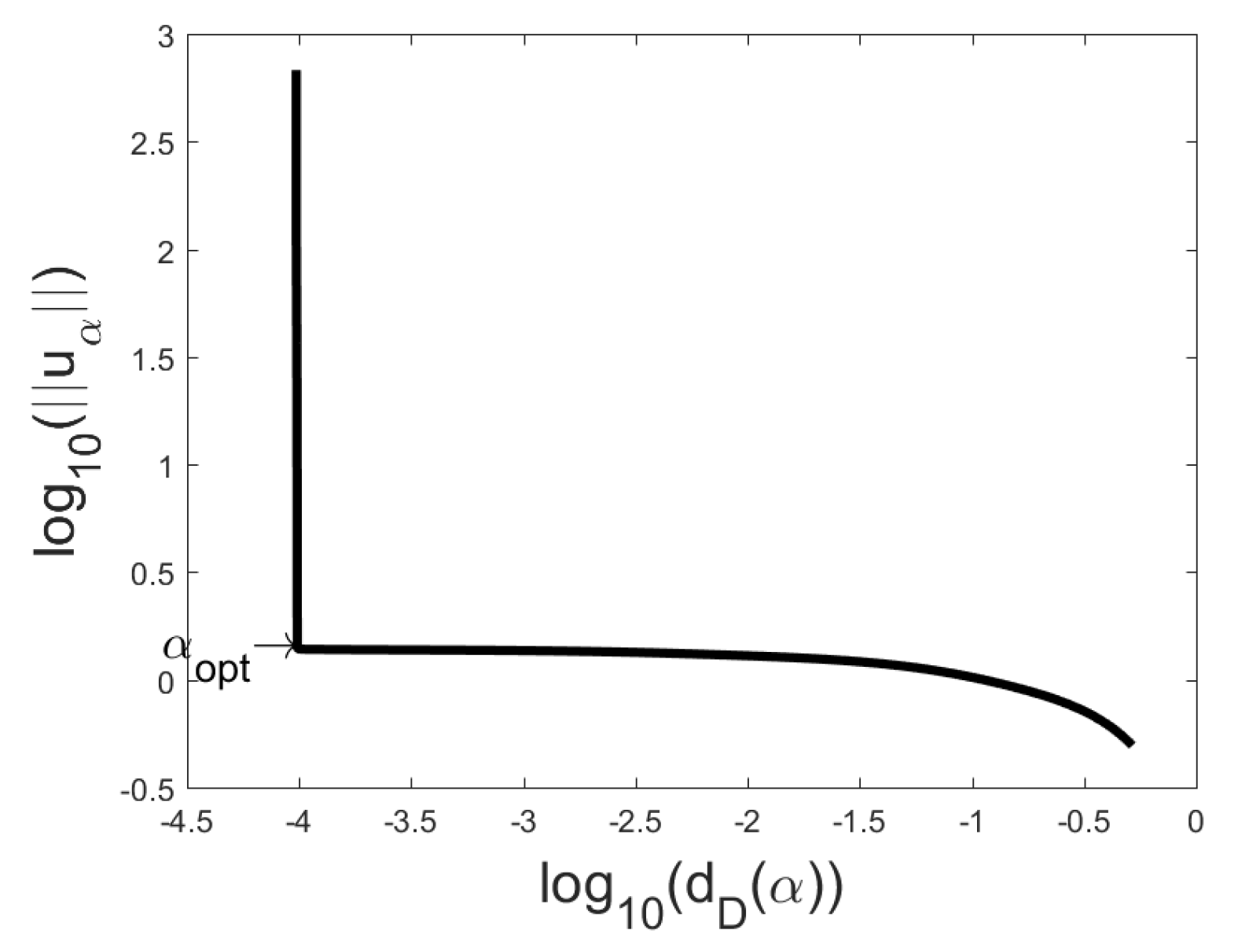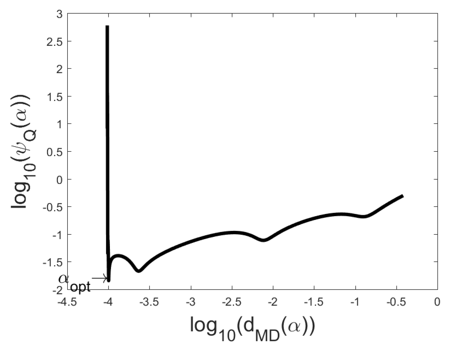For many problems the curve $({\tilde{d}}_{\mathrm{MD}}(\alpha ),{\tilde{\psi }}_{\mathrm{Q}}(\alpha ))$ (or a part of this) has the form of letter L or V and we choose the minimizer at the “corner” point of L or V. We use the common logarithm instead of the natural logarithm, while then the Q-curve allows easier estimation of the supposed value of the noise level. In Figure 1, Figure 2, Figure 3, Figure 4, Figure 5, Figure 6, Figure 7 and Figure 8 $n=100$ is used, in Figure 9 and Figure 10 $n=60$. 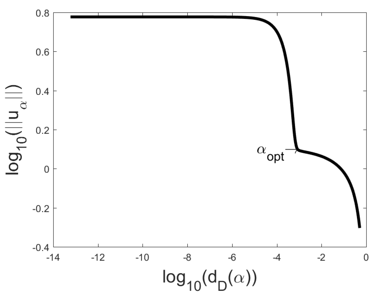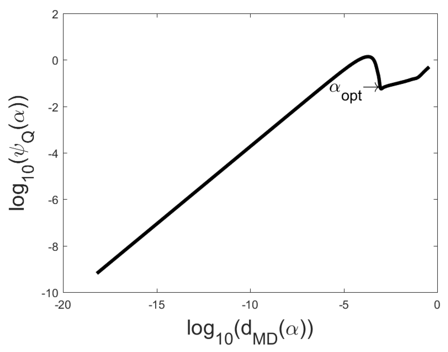In Figure 1, Figure 2, Figure 3 and Figure 4 the L-curves and Q-curves are compared for two problems, the global minimizer ${\alpha }_{opt}$ of the function $e_1(\alpha )$ is also presented. Note that in problem Baart ${\lambda }_{\min }<{\alpha }_N$ and in problem Deriv2 ${\lambda }_{\min }>{\alpha }_N$.

In most cases one can see on the Q-curve only one clear corner area with one local minimizer and then we take this local minimizer as corner point. If the corner area contains several local minimizers, we recommend to choose such local minimizer, for which the sum of coordinates of the corresponding point on the Q-curve is minimal. If Q-curve has several corner areas we recommend to use the very right of them. Actually, it is useful to present in the parameter choice besides the figures for every local minimizer $m_k$ of the function ${\psi }_{\mathrm{Q}}(\alpha )$ also the coordinates of the point $({\tilde{d}}_{\mathrm{MD}}(m_k),{\tilde{\psi }}_{\mathrm{Q}}(m_k))$ and the sums of the coordinates.

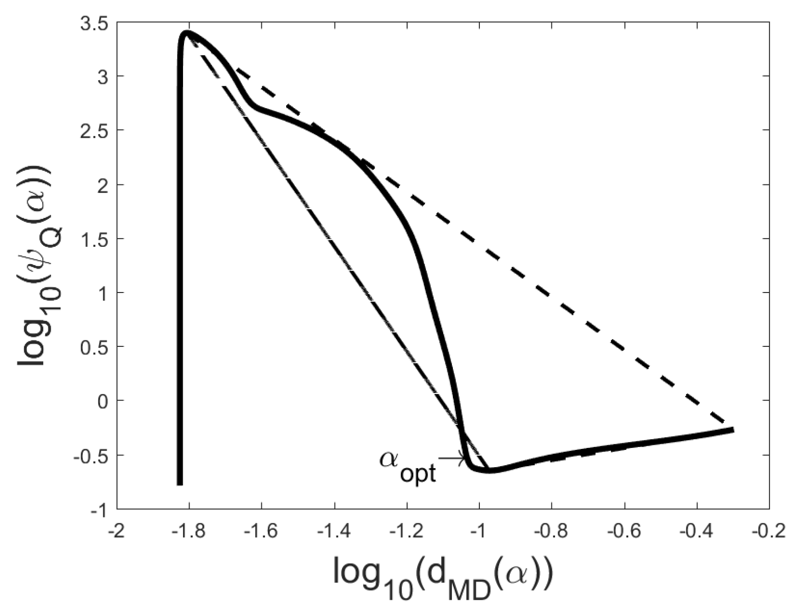
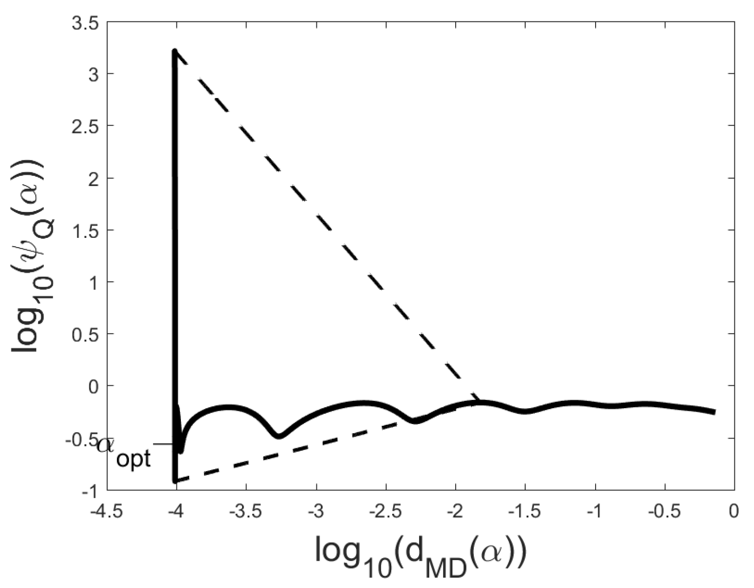
For finding the proper local minimizer of the function ${\psi }_{\mathrm{Q}}(\alpha )$ we present now a rule which works well for all test problems from set 1. The idea of the rule is to search the proper local minimizer $m_k$ constructing certain triangles on the Q-curve and finding which of them has the maximal area. For every parameter $\alpha$ corresponds a point $P(\alpha )$ on the Q-curve with the corresponding coordinates $\left({\tilde{d}}_{\mathrm{MD}}(\alpha ),{\tilde{\psi }}_{\mathrm{Q}}(\alpha )\right)$. For every local minimizer $m_k$ of the function ${\psi }_{\mathrm{Q}}(\alpha )$ corresponds a triangle $T(k,r(k),l(k))$ with the vertices $P(m_k),P(M_{r(k)})$ and $P(M_{l(k)})$ on the Q-curve, where indices $r(k)$ and $l(k)$ correspond to the largest local maximums of the function ${\psi }_{\mathrm{Q}}(\alpha )$ on two sides of the local minimum $m_k$:

$${\psi }_{\mathrm{Q}}(M_{r(k)})=\underset{j<k}{max}{\psi }_{\mathrm{Q}}(M_j),{\psi }_{\mathrm{Q}}(M_{l(k)})=\underset{j\ge k}{max}{\psi }_{\mathrm{Q}}(M_j).$$

Triangle area rule (TA-rule). We choose for the regularization parameter such local minimizer $m_k$ of the function ${\psi }_{\mathrm{Q}}(\alpha )$ for which the area of the triangle $T(k,r(k),l(k))$ is the largest.

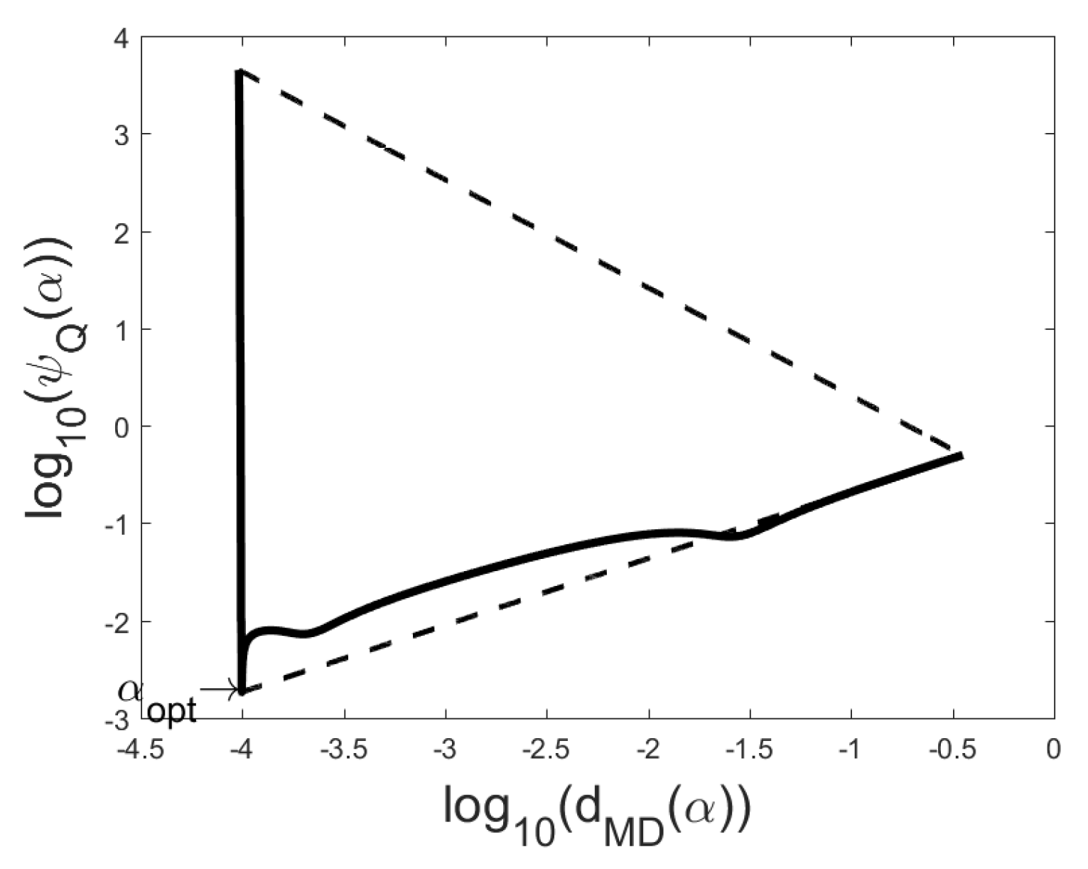
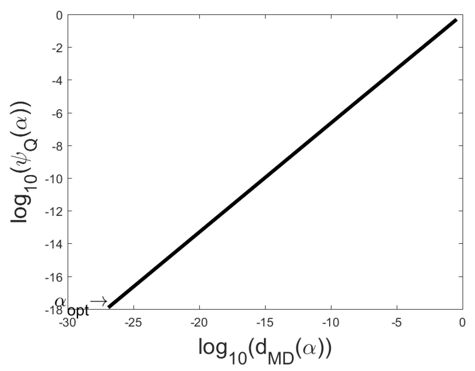
Figure 5, Figure 6 and Figure 7 show examples of Q-curves and the triangle $T(k,r(k),l(k))$ with the largest area, the TA-rule chooses for the regularization parameter a corresponding minimizer. In some problems the function ${\psi }_{\mathrm{Q}}(\alpha )$ may be monotonically increasing as for the problem Groetsch2 (Figure 8), then function ${\psi }_{\mathrm{Q}}(\alpha )$ has only one local minimizer ${\alpha }_N$. Then vertices $P(M_{l(k)})$ and $P(m_k)$ coincide and the area of the corresponding triangle is zero. Then this is the only triangle, the TA-rule chooses for the regularization parameter ${\alpha }_N$. The results of the numerical experiments for test set 1 ($n=100$ ) for the TA-rule and some other rules (see Section 2.2) are given in

Table 4. Averages of error ratios E and failure % (in parenthesis) for heuristic rules.

Problem	TA Rule		Quasiopt.	WQ	HR	Reginska	MCurv
	Mean E	Max E	Mean E	Mean E	Mean E	Mean E	Mean E
Baart	1.51	14.57	1.54	1.43	2.58	1.32	4.75
Deriv2	1.18	1.27	2.01	2.26	2.28	3.67	(9.2%)
Foxgood	1.56	3.39	1.57	1.57	8.36	(10.8%)	5.95
Gravity	1.14	2.27	1.13	1.13	2.66	(0.8%)	2.04
Heat	1.26	1.34	(65.8%)	(66.8%)	1.64	(4.2%)	4.11
Ilaplace	1.24	2.34	1.24	1.22	1.94	1.66	2.99
Phillips	1.07	1.20	1.09	(3.3%)	2.27	(44.2%)	1.34
Shaw	1.42	8.96	1.43	1.41	2.34	1.80	4.64
Spikes	1.01	5.75	1.01	1.01	1.03	1.01	1.05
Wing	1.39	6.63	1.40	1.30	1.51	1.18	1.57
Baker	3.30	11.33	3.30	3.30	(0.8%)	(21.7%)	7.78
Ursell	2.87	31.06	3.54	2.35	4.71	1.86	7.54
Indramm	3.74	9.07	4.43	4.16	(2.5%)	(9.2%)	(15.8%)
Waswaz2	2.43	9.01	2.43	2.43	(65.8%)	2.33	(3.3%)
Groetsch1	1.14	4.56	1.14	1.12	1.61	1.26	1.52
Groetsch2	1.13	1.74	1.27	2.73	1.66	5.49	1.81
Total	1.71	31.06	>100	>100	50.5	43.8	8.17
Failure %	0%		4.11%	4.38%	4.32%	5.68%	1.77%
Max E2	2.61		>100	>100	2.63	>100	24.5

and

Table 5. Distribution of error ratios E in different rules.

Decile	TA Rule	Quasiopt.	WQ	HR	Reginska	MCurv	ME	MEe	DP
10	1.00	1.00	1.00	1.08	1.00	1.06	1.01	1.00	1.00
20	1.01	1.01	1.01	1.36	1.04	1.27	1.03	1.00	1.01
30	1.02	1.03	1.03	1.56	1.12	1.48	1.09	1.01	1.02
40	1.04	1.06	1.06	1.82	1.27	1.83	1.16	1.03	1.04
50	1.09	1.13	1.12	2.12	1.66	2.31	1.22	1.08	1.08
60	1.18	1.29	1.29	2.43	2.42	3.05	1.33	1.16	1.16
70	1.35	1.57	1.59	3.19	4.19	4.51	1.52	1.29	1.30
80	1.71	2.17	2.29	5.94	9.93	7.03	2.02	1.50	1.52
90	2.27	6.45	6.18	19.35	43.91	12.95	4.45	2.88	2.11

. These results show that the TA-rule works well in all these test problems, the accuracy is comparable with $\delta$-rules (see Table 3), but previous heuristic rules fail in some problems. Note that average of the error ratio increases for decreasing noise level. For example, for $∥f-f_{*}∥\in \{{10}^{-1},{10}^{-2},{10}^{-5},{10}^{-6}\}$ corresponding error ratios E were 1.47, 1.49, 1.78 and 2.08 respectively.

Let us comment on other heuristic rules. The accuracy of the quasi-optimality criterion is for many problems the same as for the TA-rule, but this rule fails in problem Heat. A characteristic feature of the problem Heat is that location of the eigenvalues in the interval $[{\alpha }_N,1]$ is sparse and only some eigenvalues are smaller than ${\alpha }_N$ (see Table 1). The weighted quasioptimality criterion behaves in a similar way as the quasioptimality criterion, but is more accurate in problems where ${\lambda }_{\min }\le {\alpha }_N$; if ${\lambda }_{\min }>{\alpha }_N$, the quasioptimality criterion is more accurate. The rule of Hanke–Raus may fail in test problems with large $\Lambda$ and for other problems the error of the approximate solution is in most problems approximately two times larger than for parameter chosen by the quasi-optimality principle. The problem in this rule is that it chooses too large parameter compared with the optimal parameter. However, HR-rule is stable in the sense that the largest error ratio E2 is relatively small in all considered test problems. Reginska’s rule may fail in many problems but it has the advantage that it works better than other previous rules if the noise level is large. The Reginska’s rule did not fail in case $∥f-f_{*}∥\ge {10}^{-3}$ and has average of error ratios of all problems $E=2.24$ and $E=2.80$ in cases $∥f-f_{*}∥={10}^{-1}$ and $∥f-f_{*}∥={10}^{-2}$, respectively. Advantage of the maximum curvature rule is the small percentage of failures compared with other previous rules.

Distribution of error ratios E in Table 5 show also that in test problems set 1 the TA-rule is the most accurate rule from all considered rules.

Note that the figure of the Q-curve enables to estimate the reliability of the chosen parameter. If the Q-curve has only one corner, then the chosen parameter is quasioptimal with small constant C, if ${\lambda }_{\min }<{\alpha }_N$, but in case ${\lambda }_{\min }\ge {\alpha }_N$ it is quasioptimal under assumption that the problem needs regularization.

6. Further Developments of the Area Rule

The TA-rule may fail for problems which do not need regularization, if function ${\psi }_{\mathrm{Q}}(\alpha )$ is not monotonically increasing. In this case, the TA rule selects the parameter $\alpha \ge {\lambda }_{\min }$, but the parameter $\alpha <{\lambda }_{\min }$ would be better. For example, the TA-rule fails for matrix Moler in some cases. Let us consider now the question, in which cases the regularization parameter ${\alpha }_N$ is good. If function ${\psi }_{\mathrm{Q}}(\alpha )$ is monotonically increasing then function ${\psi }_{\mathrm{Q}}(\alpha )$ has only one local minimizer $m_1=M_1={\alpha }_N$ and then for the parameter ${\alpha }_N$ we have the error estimate

$$∥u_{{\alpha }_N}-u_{*}∥\le q^{-1}(1+T({\alpha }_N))\underset{{\alpha }_N\le \alpha \le {\alpha }_0}{min}{e}_1(\alpha ),$$

where the value of $T({\alpha }_N)={max}_{{\alpha }_j\in \Omega ,{\alpha }_N\le {\alpha }_j\le {\alpha }_0}T\left({\alpha }_N,{\alpha }_j\right)\le c_{q}ln(\frac{{\alpha }_0}{{\alpha }_N})$ (see Theorem 3) can be computed a posteriori and this value is the smaller the faster the function ${\psi }_{\mathrm{Q}}(\alpha )$ increases. We can take ${\alpha }_N$ for the regularization parameter also in the case if the condition

$$\frac{{\psi }_{\mathrm{Q}}({\alpha }^{\prime })}{{\psi }_{\mathrm{Q}}(\alpha )}\le c_0\forall \alpha ,{\alpha }^{\prime }\in \Omega ,{\alpha }_N\le {\alpha }^{\prime }<\alpha \le {\alpha }_0$$

(20)

holds while one can show similarly to the proof of Theorem 3 that $T({\alpha }_N)\le c_0{c}_{q}ln(\frac{{\alpha }_0}{{\alpha }_n})$ and the error of the regularized solution is small. For the problems which do not need regularization we can improve the performance of the TA-rule searching the proper local minimizer smaller or equal than ${\alpha }_{\mathrm{HQ}}:=max\{{\alpha }_{\mathrm{HR}},{\alpha }_{\mathrm{Q}}\},$ where ${\alpha }_{\mathrm{HR}}$, ${\alpha }_{\mathrm{Q}}$ are the global minimizers of functions ${\psi }_{\mathrm{HR}}(\alpha )$ and ${\psi }_{\mathrm{Q}}(\alpha )$, respectively on the interval $[max\left({\alpha }_N,{\lambda }_{\min }\right),{\alpha }_0]$.

These ideas enable to formulate the following upgraded version of the TA-rule.

Triangle area rule 2 (TA-2-rule). We fix a constant $c_0,1\le c_0\le 2$. If condition (20) holds, we choose the parameter ${\alpha }_N$. Otherwise choose for the regularization parameter such local minimizer $m_k\le {\alpha }_{\mathrm{HQ}}$ of the function ${\psi }_{\mathrm{Q}}(\alpha )$ for which the area of triangle $T(k,r(k),l(k))$ is largest.

Results of numerical experiments for the rule TA-2 with the discretization parameter $n=100$ and problem sets 1–3 are given in

Table 6. Averages and maximums of error ratios E in case of area rules, problem set 1.

Problem	TA-2 Rule		Area Rule 2		Area Rule 3		Combined Area Rule
	Aver E	Max E	Aver E	Max E	Aver E	Max E	Aver E	Max E
Baart	1.51	5.18	1.58	2.91	1.59	2.91	1.53	5.18
Deriv2	1.12	1.42	1.12	1.42	1.12	1.42	1.12	1.42
Foxgood	1.57	6.69	1.53	6.19	1.53	6.19	1.57	6.69
Gravity	1.17	4.12	1.21	6.10	1.21	6.10	1.17	4.12
Heat	1.12	2.36	1.12	2.36	1.12	2.36	1.12	2.36
Ilaplace	1.24	2.68	1.22	2.68	1.22	2.68	1.24	2.68
Phillips	1.07	1.72	1.06	1.72	1.06	1.72	1.07	1.72
Shaw	1.42	3.72	1.47	3.64	1.47	3.64	1.42	3.72
Spikes	1.01	1.05	1.01	1.02	1.01	1.02	1.01	1.05
Wing	1.39	1.86	1.44	1.86	1.44	1.86	1.39	1.86
Baker	3.30	45.29	2.67	22.67	2.67	22.67	2.91	33.12
Ursell	2.87	16.78	4.55	27.92	4.55	27.92	3.12	16.78
Indramm	3.74	25.67	9.50	83.20	10.76	83.20	3.87	25.67
Waswaz2	2.43	9.01	2.43	9.01	2.43	9.01	2.43	9.01
Groetsch1	1.14	2.12	1.15	2.12	1.15	2.12	1.14	2.12
Groetsch2	1.52	3.84	1.52	3.84	1.52	3.84	1.52	3.84
Total	1.73	45.29	2.16	83.20	2.22	83.20	1.73	33.12

and

Table 7. Averages and maximums of error ratios E in proposed rules, problem sets 2 and 3.

Problem	TA-2 Rule		Area Rule 2		Area Rule 3		Combined Area Rule
	Aver E	Max E	Aver E	Max E	Aver E	Max E	Aver E	Max E
Gauss	1.24	5.05	1.26	6.56	1.26	6.56	1.24	5.05
Hilbert	1.46	7.25	1.83	21.22	1.81	21.22	1.46	7.25
Lotkin	1.47	11.17	1.91	18.66	1.88	11.17	1.47	11.17
Moler	1.51	7.35	1.43	7.35	1.43	7.35	1.51	7.35
Prolate	1.57	15.96	1.82	20.64	1.77	15.96	1.58	15.96
Pascal	1.04	1.13	1.06	1.18	1.06	1.18	1.05	1.18
Set 2	1.38	15.96	1.55	21.22	1.53	21.22	1.39	15.96
Set 3	1.85	136.6	2.81	188.1	2.77	188.1	2.02	153.5

(columns 2 and 3). The results show that the rule TA-2 works well in all considered testsets 1–3. However, the rule TA-2 may fail in some other problems which do not need regularization. Such example is the problem with matrix moler and solution $x_i=sin(12\pi (i-1)/n)$, where the rule TA-2 fails if the noise level is below ${10}^{-4}$; but in this case all other considered heuristic rules fail too.

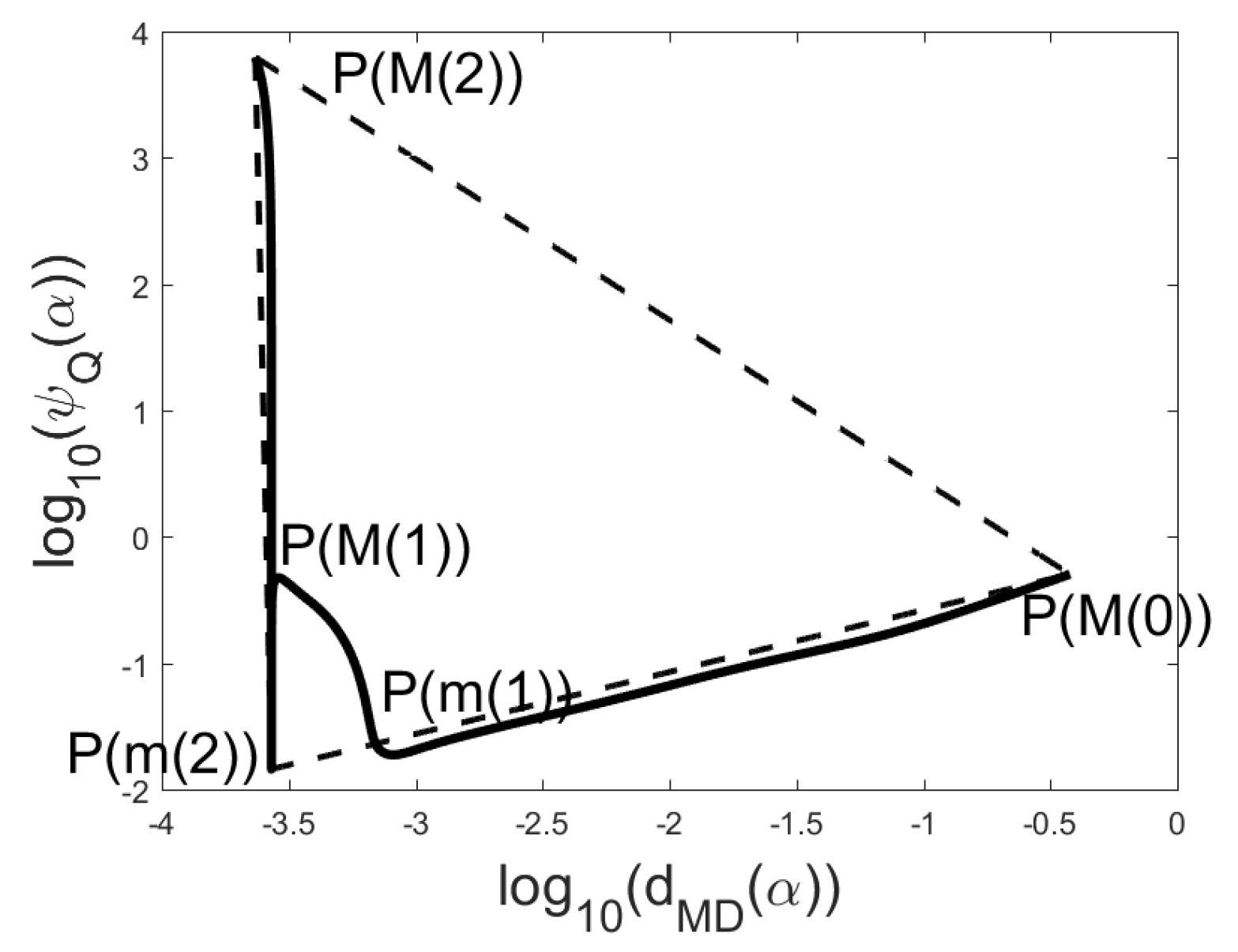
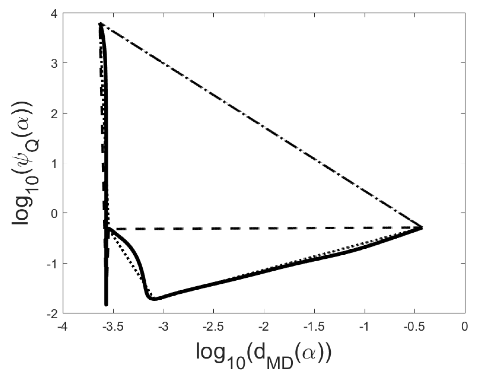
The rules TA and TA-2 fail in problem Heat in some cases for the discretization parameter $n=60$. Figure 9 and Figure 10 show the form of the Q-curve in problem Heat with $n=60$. The function ${\psi }_{\mathrm{Q}}(\alpha )$ has two local minimizers with corresponding points $P(m_1)$ and $P(m_2)$ on the Q-curve and 3 local maximum points $P(M_k),k=0,1,2$. On Figure 9 the Rule TA-2 chooses the local minimizer corresponding to the point $P(m_2)$, but then the error ratios are large: $E=20.3,E2=18.34$.

In the following we consider methods which work well also in this problem. Let $g[{\alpha }_1,{\alpha }_2](\alpha ),\alpha \in [{\alpha }_1,{\alpha }_2]$ be the parametric representation of the straight line segment connecting points $P({\alpha }_1)$ ja $P({\alpha }_2)$, thus

$$g[{\alpha }_1,{\alpha }_2](\alpha )={\tilde{\psi }}_{\mathrm{Q}}({\alpha }_1)+\beta ({\tilde{d}}_{\mathrm{MD}}(\alpha )-{\tilde{d}}_{\mathrm{MD}}({\alpha }_1)),\beta =\frac{{\tilde{\psi }}_{\mathrm{Q}}({\alpha }_2)-{\tilde{\psi }}_{\mathrm{Q}}({\alpha }_1)}{{\tilde{d}}_{\mathrm{MD}}({\alpha }_2)-{\tilde{d}}_{\mathrm{MD}}({\alpha }_1)}.$$

Let $g[{\alpha }_1,{\alpha }_2,\dots ,{\alpha }_k](\alpha )$, $k>2$ be the parametric representation of the broken line connecting points $P({\alpha }_1)$, $P({\alpha }_2),\dots ,P({\alpha }_k)$, thus

$$g[{\alpha }_1,{\alpha }_2,\dots ,{\alpha }_k](\alpha )=g[{\alpha }_j,{\alpha }_{j+1}](\alpha ),{\alpha }_j\le \alpha \le {\alpha }_{j+1},1\le j\le k-1.$$

In the triangle rule certain points $P(M_{l(k)}),P(m_k),P(M_{r(k)})$ are connected by the broken line $t_1(\alpha )=g[M_{l(k)},m_k,M_{r(k)}](\alpha )$ which approximates the error function ${\tilde{e}}_1(\alpha )={log}_{10}(e_1(\alpha ))$ well, if $m_k$ is the “right” local minimizer. By construction of the function $t_1(\alpha )$ we use only 3 points on the Q-curve. We will get a more stable rule if the form of the Q-curve has more influence to the construction of approximates to the error function ${\tilde{e}}_1(\alpha )$. Let $\{i(1),i(2),\dots ,i(n1)\}$ and $\{j(1),j(2),\dots ,j(n2)\}$ be the largest sets of the indices, satisfying the inequalities

$$k\le i(1)<i(2)<\dots <i(n1)\le K,{\psi }_{\mathrm{Q}}(M_{i(1)})\le {\psi }_{\mathrm{Q}}(M_{i(2)})\le \dots \le {\psi }_{\mathrm{Q}}(M_{i(n1)}),$$

$$k>j(1)>j(2)>\dots >j(n2)\ge 0,{\psi }_{\mathrm{Q}}(M_{j(1)})\le {\psi }_{\mathrm{Q}}(M_{j(2)})\le \dots \le {\psi }_{\mathrm{Q}}(M_{j(n2)}).$$

It is easy to see that $i(n1)=l(k)$ and $j(n2)=r(k)$. For approximating the error function ${\tilde{e}}_1(\alpha )$ we propose to connect points $P(M_{i(n1)}),\dots ,P(M_{i(1)}),P(m_k),P(M_{j(1)}),\dots ,P(M_{j(n2)})$ by the broken line $t_2(\alpha )=g[M_{i(n1)},\dots ,M_{i(1)},m_k,M_{j(1)},\dots ,M_{j(n2)}](\alpha )$ and to find for every $m_k$ the area $S_2(k)$ of the polygon surrounded by the lines $T_2(\alpha )=max\{t_2(\alpha ),g[M_{i(n1)},M_{j(n2)}](\alpha )\}$ and $t_2(\alpha )$. The second possibility is to approximate the error function ${\tilde{e}}_1(\alpha )$ by the curve $t_3(\alpha )=max\{t_2(\alpha ),{\tilde{\psi }}_{\mathrm{Q}}(\alpha )\}$ and to find $S_3(k)$ as the area of the polygon surrounded by the broken lines $t_3(\alpha )$ and curve $T_3(\alpha )=max\{T_2(\alpha ),{\tilde{\psi }}_{\mathrm{Q}}(\alpha )\}$. Note that functions $t_i(\alpha ),i=1,2,3$ are monotonically increasing if $\alpha >m_k$, and monotonically decreasing if $\alpha <m_k$.

Area rules 2 and 3. We fix a constant $c_0,1\le c_0\le 2$. First we choose the local minimizer $m_k\le {\alpha }_{HQ}$, for which the area $S_i(k),i\in \{2,3\}$ is largest. We take for the regularization parameter the smallest $m_{k_0}\le m_k$, satisfying condition (compare with (20))

$$\frac{{\psi }_{\mathrm{Q}}({\alpha }^{\prime })}{{\psi }_{\mathrm{Q}}(\alpha )}\le c_0\forall \alpha ,{\alpha }^{\prime }\in \Omega ,m_{k_0}\le {\alpha }^{\prime }<\alpha \le m_k.$$

Let us consider Figure 9. The reason for the failure of the triangle rule is, that for the local minimizer $m(2)$ the broken line $g[M(0),m(2),M(2)](\alpha )$ do not approximate well the function ${\tilde{e}}_1(\alpha )$, while point $M(1)$ is located above the interval $[m(2),M(0)]$. Here the function ${\tilde{e}}_1(\alpha )$ is better approximated by the broken line $g[M(0),M(1),m(2),M(2)](\alpha )$, see Figure 10. For the local minimizer $m(1)$, we approximate function ${\tilde{e}}_1(\alpha )$ by the broken line $g[M(0),m(1),M(1),M(2)](\alpha )$ and due to the inequality $S_2(1)>S_2(2)$ the area rule 2 chooses $m_1$ for the regularization parameter, then $E=1.05$.

The area rules 2 and 3 work in problem Heat well for every n and all ${\alpha }_N={10}^{-k},12\le k\le 24$, but in some other problems the accuracy of the area rules 2 and 3 (see columns 4–7 of Table 6 and Table 7) is slightly worse than for the rule TA-2. The advantage of the area rule 3, as compared to the area rule 2, is to be highlighted in problem Heat if all noise of the right hand side is placed on one eigenelement (then we use the condition $m_k\le {\alpha }_{HQ}$ only in case ${\lambda }_{\min }>{\alpha }_N$). Then the area rule 3 did not fail if $n\ge 80$ and ${\alpha }_N\le {10}^{-20}$. So we can say, the more precisely we take into account the form of the Q-curve in construction of the approximating function for the error function ${\tilde{e}}_1(\alpha )$, the more stable is the rule.

Based on the above rules it is possible to formulate a combined rule, which chooses the parameter according to the rule TA-2 or area rule 3 in dependence of certain condition.

Area rule 4 (Combined area rule). Fix a constant $c_0,1\le c_0\le 2,b\ge 0$. Let the local minimizer $m_k$ be chosen by the rule TA-2. If

$$\underset{m_k\le \alpha \le M_{r(k)}}{max}\frac{{\tilde{\psi }}_{\mathrm{Q}}(\alpha )}{g[m_k,M_{r(k)}](\alpha )}\le b,$$

we take $m_k$ for the regularization parameter, otherwise we choose the regularization parameter by the area rule 3.

Note that the combined rule coincides with the rule TA-2, if $b=0$ and with the area rule 3, if $b=\infty$. Experiments of combined rule with $c_0=2,b=1$ (columns 8 and 9 in Table 6 and Table 7) show that the accuracy of this rule is almost the same as in the triangle rule, but unlike the TA-2 rule, it works well also in problem Heat for all n and ${\alpha }_N$. Although, in some cases, in test set 3 the error ratio $E>100$ for rule 4, the high qualification of the rule is characterized by the fact, that over all problems sets 1–3 the largest error ratio E1 was 16.91 (5.06 for set 1) and the largest error ratio E2 was 4.67 (2.62 for set 1). Numerical experiments show that it is reasonable to use parameter $b\in (0.8,1.2]$. We studied the behavior of the area rules for different ${\alpha }_N={10}^{-k},12\le k\le 24$. The results were similar to the results of Table 6 and Table 7, but for smaller ${\alpha }_N$ the error ratios were 2–3% smaller than for ${\alpha }_N={10}^{-18}$ and for larger ${\alpha }_N$ the error ratios were about 5% larger than in Table 6 and Table 7.

The Table 2 gives results of the numerical experiments in the case of smooth solution, $p=2$. We see that combined rule worked well also in this case, no failure.

Remark 5.

It is possible to modify the Q-curve. We may use the function ${\psi }_{\mathrm{QD}}(\alpha )$ instead of function ${\psi }_{\mathrm{Q}}(\alpha )$ and find proper local minimizer of the function ${\psi }_{\mathrm{QD}}(\alpha )$. Unlike the quasi-optimality criterion the use of function ${\psi }_{\mathrm{QD}}(\alpha )$ in the Q-curve and in the area rule does not increase the amount of calculations, while approximation $u_{2,\alpha }$ is needed also in computation of $d_{\mathrm{MD}}(\alpha )$. We can use in these rules the function $d_{\mathrm{ME}}(\alpha )$ instead of $d_{\mathrm{MD}}(\alpha )$, it increases the accuracy in some problems, but the average accuracy of the rules is almost the same. In case of nonsmooth solutions we can modify the Q-curve method and area rule, using the function $d_D(\alpha )$ instead of $d_{\mathrm{MD}}(\alpha )$. In this case, we get even better results for $p=0$ but for $p=2$, the error ratio E is on average 2 times higher.

Note that if the solution is smooth, then L-curve rule and Reginska’s rule often fail, but replacing in these rules the function $A{u}_{\alpha }-f$ by the function $B_{\alpha }(A{u}_{\alpha }-f)$ gives often better results.

Remark 6.

If the solution is smooth, then using α-s from (8) much better approximate solution than single Tikhonov approximation may be get using the linear combinations of Tikhonov approximations, see [40].

In the case of a heuristic parameter choice, it is also possible to use the a posteriori estimates of the approximate solution, which, in many tasks, allows to confirm the reliability of the parameter choice. Let ${\alpha }_H$ be the regularization parameter from some heuristic rule and ${\alpha }_{*}$ be the local minimizer of the function $e_1(\alpha )$ on the set $\Omega$. Then in the case ${\alpha }_{*}\ge {\alpha }_H$ the error estimate

$$∥u_{{\alpha }_H}-u_{*}∥\le \left(1+T({\alpha }_H,{\alpha }_{*})\right)e_1({\alpha }_{*})\le q^{-1}\left(1+T_1({\alpha }_H)\right)\underset{\alpha }{min}{e}_1(\alpha )$$

(21)

holds where $T_1({\alpha }_H)={max}_{\alpha \ge {\alpha }_H,\alpha \in \Omega }T({\alpha }_H,\alpha )$. Using the last estimate, we can prove similarly to the Theorem 7 that if ${\alpha }_N$ is so small that $d_{\mathrm{MD}}({\alpha }_N)\le (1+ϵ)∥f-f_{*}∥$, then

$$∥u_{{\alpha }_H}-u_{*}∥\le max\{q^{-1}(1+T_1({\alpha }_H))\underset{\alpha \ge 0}{min}{e}_1(\alpha ),C_2(b,ϵ)\underset{\alpha \ge 0}{min}{e}_2(\alpha ,∥f-f_{*}∥)\},$$

where $b=d_{\mathrm{MD}}({\alpha }_H)/d_{\mathrm{MD}}({\alpha }_N)$. If values $T_1({\alpha }_H)$ and b, what we find a posteriori, are small (for example $b\le 2$ and $T_1({\alpha }_H)\le 9$), then this estimate allows to argue that the error of the approximate solution for this parameter is not much larger than the minimal error. The conditions $b\le 2$, $T_1({\alpha }_H)\le 9$ were satisfied in set 1 of test problems in the combined rule for 73% of cases and inequalities $b\le 2$, $T_1({\alpha }_H)\le 4$ for 61% of cases. The reason of failure of heuristic rule is typically that the chosen parameter is too small. To check this, we can use the error estimate (21). If $T_1({\alpha }_H)$ is relatively small (for example $T_1({\alpha }_H)\le 9$), then the estimate (21) allows to argue that the regularization parameter is not chosen too small. In set 1 of test problems the conditions $T_1({\alpha }_H)\le 9$ and $T_1({\alpha }_H)\le 4$ were satisfied in 97% and in 82% of cases, respectively.

7. Conclusions

We finish the paper with the following conclusion. For the heuristic choice of the regularization parameter we recommend to choose the parameter from the set of local minimizers of the function ${\psi }_{\mathrm{Q}}(\alpha )$ or the function ${\psi }_{\mathrm{QD}}(\alpha )$. For choice of the parameter from the local minimizers we proposed the Q-curve method and different area rules. The proposed rules gave much better results than previous heuristic rules on extensive set of test problems. Area rules fail in very few cases in comparison with previous rules, and the accuracy of these rules is comparable even with the $\delta$-rules if the exact noise level is known. In addition, we also provided a posteriori error estimates of the approximate solution, which allows to check the reliability of parameter chosen heuristically.