Purely Iterative Algorithms for Newton’s Maps and General Convergence

Abstract

The aim of this paper is to study the local dynamical behaviour of a broad class of purely iterative algorithms for Newton’s maps. In particular, we describe the nature and stability of fixed points and provide a type of scaling theorem. Based on those results, we apply a rigidity theorem in order to study the parameter space of cubic polynomials, for a large class of new root finding algorithms. Finally, we study the relations between critical points and the parameter space.

1. Introduction

The computation of solutions for equations of the form

$$\mathsf{\Psi }(x)=\alpha ,$$

is a classic problem that arises in different areas of mathematics and in particular in numerical analysis. Here $\mathsf{\Psi }:\mathbb{C}\to \mathbb{C}$ is a complex function, and usually it is assumed that $\alpha =0$. Due to the dependence on the space where the equation is defined, and where possible solutions are acting, it is ambitious to expect a unified theory that provides the exact, or even approximate solutions to this class of equations. Also, depending on the objective that is being addressed, solving an equation as above can be very different in nature, as well as, the techniques used to solve it. For instance, Picard–Lindelöf’s theorem (see for example [1]) on existence and uniqueness of solutions of ordinary differential equations, and fundamental theorem of Algebra in complex analysis. On the other hand, if we turn our attention to explicit solutions, then the problem becomes even more difficult.

Consider a complex polynomial f and

$${\displaystyle N_f=Id-\frac{f}{f^{\prime }}}$$

the classical Newton’s method. In this case, higher–order methods have been extensively used and studied in order to approach the equation $f(z)=0.$ The iterative function $N_f$ defines a rational map on the extended complex plane (Riemann sphere) $\overline{\mathbb{C}}=\mathbb{C}\cup \{\infty \}$. The simple roots of the equation $f(z)=0$, or in other words, the roots of the equation $f(z)=0$ that are not roots of the derivative $f^{\prime }(z)$, are super–attracting fixed points of $N_f$, that is, let $\zeta$ be a simple root of $f(z)$, then $N_f(\zeta )=\zeta$ and $N_f^{\prime }(\zeta )=0$. For a review of the dynamics of Newton’s method, see for instance [2,3].

More generally, $Pol{y}_d$ and $Ra{t}_k$ denote the space of polynomials of degree d and the space of rational functions of degree k, respectively. By a root–finding algorithm or root–finding method it is meant a rational map $T_f:Pol{y}_d\to Ra{t}_k$, such that the roots of the polynomial map f are attracting fixed points of $T_f$. A root–finding algorithm $T_f$ has order $\sigma$, if the local degree of $T_f$ in every simple root of f is $\sigma$.

In this paper we study the dynamical aspects of

$$T_f(z)=z-(z-N_f(z))\frac{(a_0+a_1{N}_f^{\prime }(z)+a_2{(N_f^{\prime }(z))}^2)}{b_0+b_1{N}_f^{\prime }(z)},$$

(1)

where $a_0$, $a_1$, $a_2$, $b_0$ and $b_1$ are real numbers. Depending on those parameters, this family is of order 2, 3, 4 or 5. Also, this family can be viewed as a generalization of $c$–iterative functions (for a definition see Example 5 below).

In [4] C. Mcmullen proved a rigidity theorem that implies that a purely iterative root finding algorithm generally convergent for cubic polynomials, is conformally conjugate to a generating map. Applying this result, J. Hawkins in [5] was able to obtain an explicit expression for rational maps which are generating, and so it is natural to ask which of these rational maps $T_f$ are generating maps. We use that rigidity result in order to show that over the space of cubic polynomials, those maps $T_f$ that generate a generally convergent algorithm are restricted to Halley’s method applied to the cubic polyomial.

The paper is organized as follows. Section 2 contains some basic notions of the classic theory of complex dynamics. In addition to establish the notation and main examples, Section 3 contains the definition of purely iterative iterative algorithm for Newton’s maps, that will be used throughout the article. Section 4 is devoted to the study of the nature of fixed points. In Section 5 we study the order of convergence of $T_f$, and in Section 6 we provide the results about Scaling theorems. We provide the result concerning maps that generates generally convergent root finding algorithms for cubic polynomials in Section 7. In Section 8 we provide the relation between critical points and parameter space. The last Section summarize the conclusion.

2. Basic Notions in Complex Dynamics

We recall the reader so see [6] or [7,8,9,10,11,12,13,14,15,16] to obtain some basic notions of the classic theory of Fatou-Julia of complex dynamics which appear in (as a reference of the Fatou– Julia theory see for instance P. Blanchard [17] and J. Milnor [18]). Here we show a small summary: Let

$$R(z)=\frac{P(z)}{Q(z)}$$

be a rational map of the extended complex plane into itself, where P and Q are polynomials with no common factors.

• A point $\zeta$ is called a fixed point of R if $R(\zeta )=\zeta$, and the multiplier of R at a fixed point $\zeta$ is the complex number $\lambda (\zeta )=R^{\prime }(\zeta )$.
• Depending on the value of the mulitplier, a fixed pointcan be superattracting ($\lambda (\zeta )=0$), attracting($0<|\lambda (\zeta )|<1$), repelling($|\lambda (\zeta )|>1$), indifferent ($|\lambda (\zeta )|=1$)
• Let $z_0$ be a fixed point of $R^n$ which is not a fixed point of $R^j$, for any j with $0<j<n$. We say that $\mathrm{orb}(z_0)=\{z_0,R(z_0),\dots ,R^{n-1}(z_0)\}$ is a cycle of lengthn or simply an n–cycle. Note that $\mathrm{orb}(z_j)=\mathrm{orb}(z_0)$ for any $z_j\in \mathrm{orb}(z_0)$, and R acts as a permutation on $\mathrm{orb}(z_0)$.
• The multiplier of an $n-$ cycle is the complex number $\lambda (\mathrm{orb}(z_0))={(R^n)}^{\prime }(z_0)$.
• At each point $z_j$ of the cycle, the derivative ${(R^n)}^{\prime }$ has the same value.
• An $n-$ cycle $\{z_0,z_1,\dots ,z_{n-1}\}$ is said to be attracting, repelling, indifferent, depending the value of the associated multiplier (same conditions than in the fixed points).
• The Julia set of a rational map R, denoted $J(R)$, is the closure of the set of repelling periodic points. Its complement is the Fatou set $F(R)$. If $z_0$ is an attracting fixed point of R, then the convergence region $B(z_0)$ is contained in the Fatou set and $J(R)=\partial B(z_0)$, where ∂ denotes the topological boundary.

3. Definitions and Notations

Now we recall the definition of purely iterative algorithms due to S. Smale in [19]. Let ${\mathcal{P}}_d$ be the space of all polynomials of degree less than or equal to $d$. For every $k\ge 1$, define the space $J_k={\mathbb{C}}^{k+2}$ and the map

$$j:\mathbb{C}\times {\mathcal{P}}_d\to J_k$$

given by

$$j(z,f)=(z,f(z),f^{\prime }(z),\dots ,f^{\left[k\right]}(z)),$$

where $f^{\left[k\right]}$ denotes the kth derivative of f. Let $F:J_k\to \mathbb{C}$ be the rational map defined as

$$F(z,{\xi }_0,\dots ,{\xi }_k)=z-\frac{P(z,{\xi }_0,\dots ,{\xi }_k)}{Q(z,{\xi }_0,\dots ,{\xi }_k)},$$

(2)

where $P$ and $Q$ are polynomials in $k+2$ variables $z,{\xi }_0,\dots ,{\xi }_k$, with no common factors. A purely iterative algorithm is a rational endomorphism ${\widehat{T}}_f:\overline{\mathbb{C}}\to \overline{\mathbb{C}}$ that depends on $f\in {\mathcal{P}}_d$ and takes the form

$${\widehat{T}}_f(z)=F(j(z,f(z))),$$

(3)

for a rational map as in (2).

Consider a modification of the preceding definition. Let $Ra{t}_d$ be the space consisting of the rational maps of degree less than or equal to $d$. Define a subset $\mathcal{V}\subset Ra{t}_d$ as

$$\begin{array}{c}\mathcal{V}=\{R\in Ra{t}_d:\mathrm{finite}\mathrm{fixed}\mathrm{points}\alpha \mathrm{of}R\mathrm{are}\mathrm{simple},\frac{1}{1-R^{\prime }(\alpha )}\in \mathbb{N},\\ R(\infty )=\infty \mathrm{and}{R}^{\prime }(\infty )=d/(d-1)\}.\end{array}$$

Since Newton’s method applied to $z^d-1$ is a rational map that satisfies the conditions in $\mathcal{V}$, we conclude that $\mathcal{V}\ne \varnothing$, for every $d\ge 2$.

As above, define

$$\widehat{❚}:\overline{\mathbb{C}}\times \mathcal{V}\to J_k$$

by

$$\widehat{❚}(z,R)=(z,R(z),R^{\prime }(z),\dots ,R^{\left[k\right]}(z)).$$

Let $G:J_k\to \mathbb{C}$ be the rational map defined as

$${\displaystyle G(z,{\xi }_0,\dots ,{\xi }_k)=z-\frac{P(z,{\xi }_0,\dots ,{\xi }_k)}{Q(z,{\xi }_0,\dots ,{\xi }_k)},}$$

(4)

where $P$ and $Q$ are polynomials in $k+2$ variables with no common factors.

We define a rational endomorphism $T_f:\overline{\mathbb{C}}\to \overline{\mathbb{C}}$, depending on $R\in Ra{t}_d$, by

$$T_f(z)=G(\widehat{❚}(z,R)),$$

where $R\in \mathcal{V}$.

In [6] it is proved the following.

Theorem 1.

For every$G:J_k\to \mathbb{C}$defined as before, there exists a complex polynomial f of degree d such that for every$R\in \mathcal{V}$,$R=N_f$, where$N_f$is the Newton method. Also, there exists a linear space H of dimension$d+1$such that$\mathcal{V}$is contained in$Ra{t}_d\cap H$.

Theorem 1 motivates the following definition.

Definition 1.

Let$S_f:\overline{\mathbb{C}}\to \overline{\mathbb{C}}$be the rational endomorphism depending on$f\in {\mathcal{P}}_d$, given by

$$S_f(z)=G(\widehat{❚}(z,N_f(z)))$$

(5)

where$N_f$is Newton’s map applied to f, and G is defined by the Formula (4). A rational endomorphism $S_f$ as above will be called a purely iterative algorithm for Newton’s maps.

Remark 1.

Note that the degree of the polynomials P and Q in (4) does not depend on the degree of f.

In this paper we consider the family of purely iterative algorithm for Newton’s maps given by the Formula (5), with

$$\begin{array}{c}G(z,{\xi }_0,{\xi }_1)=z-\frac{P(z,{\xi }_0,{\xi }_1)}{Q(z,{\xi }_0,{\xi }_1)},\\ P(z,{\xi }_0,{\xi }_1)=(z-{\xi }_0)(a_0+a_1{\xi }_1+a_2{\xi }_1^2)\end{array}$$

and

$$Q(z,{\xi }_0,{\xi }_1)=b_0+b_1{\xi }_1,$$

where $a_0$, $a_1$, $a_2$, $b_0$ and $b_1$ are real numbers. Then the family is given by

$${\displaystyle T_f(z)=z-(z-N_f(z))\frac{(a_0+a_1{N}_f^{\prime }(z)+a_2{(N_f^{\prime }(z))}^2)}{b_0+b_1{N}_f^{\prime }(z)},}$$

which is exactly the Formula (1) above.

Example 1.

The family of Purely iterative algorithms for Newton’s maps (1) include several important families of root–finding algorithms.

1. 

Newton’s method is obtained by taking$a_0=b_0=1$,$a_1=a_2=b_1=0$. Indeed, in this case

$$P(z,{\xi }_0,{\xi }_1)=z-{\xi }_{0}andQ(z,{\xi }_0,{\xi }_1)=1.$$

Hence$T_f(z)=z-(z-N_f(z))=N_f(z)$. This method has been briefly studied in the last decades [20].

2. 

Halley’s method is obtained by considering$a_0=2$,$a_1=0$,$a_2=0$,$b_0=2$and$b_1=-1$. Indeed,

$$\begin{array}{cc}\hfill T_f(z)=H_f(z)& =z-2\left(\frac{z-N_f(z)}{2-N_f^{\prime }(z)}\right).\hfill \end{array}$$

Therefore,

$$P(z,{\xi }_0,{\xi }_1)=2(z-{\xi }_0)andQ(z,{\xi }_0,{\xi }_1)=2-{\xi }_1.$$

For a study of dynamical and numerical properties of Halley’s method, see for instance [21,22].

3. 

Whittaker’s iterative method also known as convex acceleration of Whittaker’s method (see [23,24]), is an iterative map of order of convergence two given by

$$\begin{array}{c}\hfill W_f(z)=z-\frac{1}{2}(z-N_f(z))\left(2-N_f^{\prime }(z)\right).\end{array}$$

Thus, according with (4) and (5), Whittaker’s method is a purely iterative algorithm for Newton’s maps when considering$k=1$, and the polynomials

$$P(z,{\xi }_0,{\xi }_1)=(z-{\xi }_0)\left(1-\frac{{\xi }_1}{2}\right)andQ(z,{\xi }_0,{\xi }_1)\equiv 1.$$

4. 

Newton’s method for multiple roots is obtained by considering$a_0=b_0=1$,$a_1=a_2=0$and$b_1=-1$. Indeed,

$$\begin{array}{cc}\hfill T_f(z)=M_f(z)& =z-\left(\frac{z-N_f(z)}{1-N_f^{\prime }(z)}\right).\hfill \end{array}$$

Note that

$$P(z,{\xi }_0,{\xi }_1)=z-{\xi }_{0}andQ(z,{\xi }_0,{\xi }_1)=1-{\xi }_1.$$

This method has been studied by several authors. See for example [25,26] and more recently [27,28].

5. 

The following method, that may be new and it is denoted by$SH{2}_f$, is a modification of the super–Halley method(for a study of this method see for instance [29]). This is given by the formula

$$SH{2}_f(z)=z-\frac{1}{2}\left(z-N_f(z)\right)\left(\frac{3-N_f^{\prime }(z)}{1-N_f^{\prime }(z)}\right).$$

Consider the polynomials

$$P(z,{\xi }_0,{\xi }_1)=\frac{1}{2}(z-{\xi }_0)(3-{\xi }_1)andQ(z,{\xi }_0,{\xi }_1)=1-{\xi }_1.$$

Again, it follows from (4) and (5) that$SH{2}_f$is a purely iterative algorithm for Newton’s maps.

6. 

More generally, considering$a_0=2$,$a_1=1-2\theta$,$a_2=0$,$b_0=2$and$b_1=-2\theta$we obtain the following third-order family studied in [30,31].

$$\begin{array}{cc}\hfill M_{f,\theta }(z)& =z-(z-N_f(z))\left(1+\frac{N_f^{\prime }(z)}{2(1-\theta N_f^{\prime }(z))}\right).\hfill \end{array}$$

In this case

$$P(z,{\xi }_0,{\xi }_1)=(z-{\xi }_0)(2-(1-2\theta {\xi }_0))andQ(z,{\xi }_0,{\xi }_1)=2-2\theta {\xi }_1.$$

7. 

The following family of iterative functions represents Newton’s method, Chebyshev’s iterative function, Halley’s method, Super-Halley, c–iterative function (considering$\theta =0$below) and Chebyshev-Halley family, among others. See for instance [22,29,30,31,32,33,34,35,36,37,38]. The family of iterative methods given by

$$\begin{array}{cc}\hfill M_{f,\theta ,c}(z)& =z-(z-N_f(z))\left(1+\frac{N_f^{\prime }(z)}{2(1-\theta N_f^{\prime }(z))}+c{(N_f^{\prime }(z))}^2\right),\hfill \end{array}$$

where θ and c are complex parameters conveniently chosen, form a family of purely iterative algorithms for Newton’s maps. Indeed, this follows by considering the polynomials

$$\begin{array}{cc}P(z,{\xi }_0,{\xi }_1)\hfill & =(z-{\xi }_0)[2(1-\theta {\xi }_1)+{\xi }_1+2c{\xi }_1(1-\theta {\xi }_1)\hfill \\ & =(z-{\xi }_0)(2+{\xi }_1(1-2\theta +2c)-2c\theta {\xi }_1^2)\hfill \end{array}$$

and

$$Q(z,{\xi }_0,{\xi }_1)=2-2\theta {\xi }_1,$$

in (4) and (5).

It is clear that$a_0=2$,$a_1=1-2(c+\theta )$,$a_2=-2c\theta$,$b_0=2$and$b_1=-2\theta$.

Remark 2.

Note that a purely iterative algorithm for Newton’s maps may not be a root–finding algorithm. For instance, by considering the polynomial$f(z)={(z-1)}^2(z+1)$, and the purely iterative Newton’s map defined by

$$P(z,{\xi }_0,{\xi }_1)=(z-{\xi }_0)(1+{\xi }_1+{\xi }_1^2)$$

and

$$Q(z,{\xi }_0,{\xi }_1)=1+b_1{\xi }_1,$$

where$b_1<-2$, it follows that root 1 is repelling for the associated rational map. In fact, in this case

$$T_f(z)=z-(z-N_f(z))\frac{(1+N_f^{\prime }(z)+{(N_f^{\prime }(z))}^2)}{1+b_1{N}_f^{\prime }(z)}.$$

Note that$T_f(1)=1$. Since$b_1<-2$then$16+8b_1<0$. Therefore

$$T_f^{\prime }(1)=1-\frac{14}{16+8b_1}>1.$$

As a consequence the root 1 is a repelling fixed point.

4. The Nature of Fixed Points

In order to ensure that $T_f$ be a root–finding algorithm (see Remark 2), some restrictions over the choice of the real parameters $a_0$, $a_1$, $a_2$, $b_0$ and $b_1$, are required. Let $m\ge 1$ be an integer and define

$${\lambda }_m=1-l_m$$

(6)

where,

$$l_m=\frac{a{m}^2-bm+a_2}{m^2(m(b_0+b_1)-b_1)}$$

and $a=a_0+a_1+a_2$ and $b=a_1+2a_2$.

Theorem 2.

Suppose that

$$0<{\lambda }_m<1$$

(7)

for every$m\ge 1$. Let$f:\mathbb{C}\to \mathbb{C}$be a complex polynomial of degree$d\ge 2$. Denote by${\alpha }_i$its zeros and by$m_i\ge 1$their multiplicities. Then$T_f$defined in (1) is a root finding algorithm. Moreover,

(a) 

Each root${\alpha }_i$of multiplicity$m_i\ge 1$is an attracting fixed point for$T_f$with multiplier${\lambda }_{m_i}=1-l_{m_i}$. Assuming that$a_0=b_0$, we have that every simple root is a superattracting fixed point for$T_f$.

(b) 

$T_f$has a repelling fixed point at ∞ with multiplier${\lambda }_d^{-1}$.

(c) 

If$a_1=a_2=0$,$b_0,b_1\ne 0$and$a_0/b_1<0$then the extraneous fixed points of$T_f$are the zeros of$f^{\prime }$which are not zeros of f. More precisely, if β is a zero of order$n\ge 2$of$f^{\prime }$, then it is a repelling fixed point of$T_f$with multiplier

$$1-\frac{a_0}{b_1(n-1)}.$$

Remark 3.

If$a_0=0$, then by Formula (6) we have that${\lambda }_1=1$, that is, the simple roots of a complex polynomial are parabolic fixed points for$T_f$. In this case$T_f$cannot be a root–finding algorithm. So, from now on,$a_0\ne 0$.

Proof. 

(a) First note that the factor $(z-N_f(z))$ in (1) implies that $T_f({\alpha }_i)={\alpha }_i$ for every i. If $f$ has a zero $\alpha$ of multiplicity $m$, then $\alpha$ is a (super)attracting fixed point of Newton’s method with multiplier $(m-1)/m$. Thus

$$N_f(z)=\alpha +(z-\alpha )\left(\frac{m-1}{m}\right)+O{(z-\alpha )}^2.$$

It follows that

$$\begin{array}{c}z-N_f(z)=\frac{1}{m}(z-\alpha )+O{(z-\alpha )}^2,\\ N_f^{\prime }(z)=\left(\frac{m-1}{m}\right)+O(z-\alpha )\mathrm{and}{(N_f^{\prime }(z))}^2={\left(\frac{m-1}{m}\right)}^2+O(z-\alpha ).\end{array}$$

Consequently,

$$\begin{array}{cc}{T}_f(z)\hfill & =\alpha +(z-\alpha )-\frac{(z-\alpha )(m^2{a}_0+a_1(m-1)m+a_2{(m-1)}^2)}{m^2(m{b}_0+b_1(m-1))}+O{(z-\alpha )}^2\hfill \\ & =\alpha +\left(1-\left(\frac{a{m}^2-bm+a_2}{m^2(m(b_0+b_1)-b_1)}\right)\right)(z-\alpha )+O{(z-\alpha )}^2\hfill \\ & =\alpha +\left(1-l_m\right)(z-\alpha )+O{(z-\alpha )}^2\hfill \end{array}$$

Consequently, $\alpha$ is an attracting fixed point with multiplier $0<1-l_m<1$. By supposing that $a_0=b_0$, we have that $l_1=1$, which implies that $\alpha$ is a superattracting fixed point.

$(b)$ Note that the degree d polynomial f can be written as

$$f(z)=\mu z^d\left(1+O\left(\frac{1}{\left|z\right|}\right)\right),$$

for some $\mu \in {\mathbb{C}}^{\ast }$. Indeed, if $f(z)=a_d{z}^d+a_{d-1}{z}^{d-1}+\cdots +a_{1}z+a_0$, then

$$f(z)=a_d{z}^d\left(1+\frac{a_{d-1}}{a_{d}z}+\cdots +\frac{a_1}{a_d{z}^{d-1}}+\frac{a_0}{a_d{z}^d}\right).$$

Therefore, when $\left|z\right|$ tends to $\infty$, it follows that $f\sim a_0{z}^d$, and we may write Newton’s method applied to the polynomial f as

$$N_f(z)=\left(\frac{d-1}{d}\right)z+O(1)\mathrm{and}{N}_f^{\prime }(z)=\left(\frac{d-1}{d}\right)+O(1).$$

By constructing the Formula (1), this implies that

$$z-N_f(z)=\left(1-\frac{d-1}{d}\right)z+O(1)=\left(\frac{1}{d}\right)z+O(1),$$

and so,

$$T_f(z)=\frac{a_0+a_1{N}_f^{\prime }(z)+a_2{(N_f^{\prime }(z))}^2}{b_0+b_1{N}_f^{\prime }(z)}=\left(\frac{a_0+\frac{a_1(d-1)}{d}+\frac{a_2{(d-1)}^2}{d^2}+O(1)}{b_0+\frac{b_1(d-1)}{d}+O(1)}\right).$$

Thus,

$$\begin{array}{cc}{T}_f(z)\hfill & =z-(z-N_f(z))\frac{(a_0+a_1{N}_f^{\prime }(z)+a_2{(N_f^{\prime }(z))}^2)}{b_0+b_1{N}_f^{\prime }(z)}\hfill \\ & =z-\left(\left(\frac{1}{d}\right)z+O(1)\right)\left(\frac{a_0+\frac{a_1(d-1)}{d}+\frac{a_2{(d-1)}^2}{d^2}+O(1)}{b_0+\frac{b_1(d-1)}{d}+O(1)}\right)\hfill \\ & =\left(1-\left(\frac{a_0{d}^2-+a_1{d}^2-a_{1}d+a_2{d}^2-2a_{2}d+a_2}{d^2(b_{0}d+b_{1}d-b_1)}\right)\right)z+O(1)\hfill \\ & =\left(1-\left(\frac{a{d}^2-bd+a_2}{d^2(d(b_0+b_1)-b_1)}\right)\right)z+O(1)\hfill \\ & =\left(1-l_d\right)z+O(1)\hfill \\ & ={\lambda }_{d}z+O(1)\hfill \end{array}$$

$(c)$ Suppose that $\beta$ is a zero of order $n\ge 2$ of $f^{\prime }$ which is not a zero of f. Then $\beta$ is a pole of order $n\ge 2$ for the map $b_0+b_1{N}_f^{\prime }$, that is,

$$b_0+b_1{N}_f^{\prime }(z)=\frac{\lambda }{{(z-\beta )}^n}+O{|z-\beta |}^{-(n-1)}.$$

This implies that

$$N_f(z)=\frac{\lambda }{b_1(1-n){(z-\beta )}^{n-1}}+O{|z-\beta |}^{-(n-2)}$$

and consequently,

$$\begin{array}{cc}{T}_f(z)\hfill & =z-\frac{a_0(z-N_f(z))}{b_0+b_1{N}_f^{\prime }(z)}\hfill \\ & =z-a_0\frac{(z-[\lambda /(b_1(1-n){(z-\beta )}^{n-1}){+O|z-\beta |}^{-(n-2)}])}{\lambda /{(z-\beta )}^n+O{|z-\beta |}^{-(n-1)}}\hfill \\ & =\beta +(z-\beta )+\frac{a_0(z-\beta )}{b_1(1-n)}+O{(z-\beta )}^2\hfill \\ & =\beta +(z-\beta )\left(1-\frac{a_0}{b_1(n-1)}\right)+O{(z-\beta )}^2,\hfill \end{array}$$

provided $m>1$. Since $b_1\ne 0$ and $a_0/b_1<0$, the quantity $1-\frac{a_0}{b_1(n-1)}$ is greater than one, and the proof is complete. □

Example 2.

Now we give some examples of Theorem 2:

1. 

Since Newton’s method is given by considering$a_0=b_0=1$,$a_1=a_2=b_1=0$, then$a=1$and$b=1$. Hence$l_m=1/m$and${\lambda }_m=1-1/m$. Thus the condition (7) is satisfied for every integer$m\ge 1$.

2. 

Halley’s method is obtained with$a=2$,$a_2=0$,$b=0$,$b_0=2$and$b_1=-1$. Then,$l_m=2/(m+1)$and${\lambda }_m=(m-1)/(m+1)$. Thus, the condition (7) is satisfied for every integer$m\ge 1$. In this case, repelling fixed point has multiplier of the form$(m+1)/(m-1)$, provided$m>1$.

3. 

In Remark 2 was considered an example of purely iterative algorithm for Newton’s maps, that is not a root-finding algorithm. In this case (7) is not satisfied when$b_1<-2$. Indeed,$l_2=14/(16+8b_1)$and${\lambda }_2=1-14/(16+8b_1)>1$, and so the condition (7) is not satisfied.

4. 

The root finding algorithm$S{H}_2$has order of convergence 3 and does not satisfy$a_0=b_0$. In this case${\lambda }_m=2/(m+1)$.

The following table summarizes the examples (1)

	${\mathit{a}}_{\mathbf{0}}$	${\mathit{a}}_{\mathbf{1}}$	${\mathit{a}}_{\mathbf{2}}$	${\mathit{b}}_{\mathbf{0}}$	${\mathit{b}}_{\mathbf{1}}$	${\mathit{\lambda }}_{\mathit{m}}$
$N_f$	$1$	$0$	$0$	$1$	$0$	$1-1/m$
$M_f$	$1$	$0$	$0$	$1$	$-1$	$0$
$H_f$	$2$	$0$	$0$	$2$	$-1$	$(m-1)/(m+1)$
$SH{2}_f$	$3$	$-1$	$0$	$2$	$-2$	$1/(2m)$
$W_f$	$2$	$-1$	$0$	$2$	$0$	$1-(m+1)/(2m^2)$

5. Order of Convergence

This section will describe the order of convergence of $T_f$ defined in (1). In this section, $N_f^{\left[n\right]}$ denote the nth derivative of Newton’s method.

Lemma 1.

Consider$T_f$as a root finding algorithm applied to a degree d polynomial f. Then:

1. 

If$a_0=b_0$, then$T_f$is at least of order 2.

2. 

If$a_0=b_0$and$b_1=a_1-\frac{a_0}{2}$, then$T_f$is at least of order 3.

3. 

If$a_0=b_0$,$b_1=a_1-\frac{a_0}{2}$,$a_1=2a_2$and$N_f^{\left[3\right]}(\alpha )=0$for every simple root α of f, then$T_f$is at least of order 4.

4. 

If condition in$(3)$is satisfied and additionally$a_1=0$and$N_f^{\left[4\right]}(\alpha )=0$for every simple root α of f, then$T_f$has order 5.

Proof. 

Recall that $a_0\ne 0$. Let $\alpha$ be a simple root of a polynomial f. Since Newton’s method is an order 2 root–finding algorithm, it follows that

$$N_f(z)=\alpha +\mu {(z-\alpha )}^2+O{(z-\alpha )}^3\mathrm{and}{N}_f^{\prime }(z)=2\mu (z-\alpha )+O{(z-\alpha )}^2,$$

for some $\mu \ne 0$. Hence,

$$\begin{array}{c}z-N_f(z)=(z-\alpha )-\mu {(z-\alpha )}^2+O{(z-\alpha )}^3,\\ {(N_f^{\prime }(z))}^2=4{\mu }^2{(z-\alpha )}^2+O{(z-\alpha )}^3.\end{array}$$

Consequently,

$$\frac{a_0+a_1{N}_f^{\prime }(z)+a_2{(N_f^{\prime }(z))}^2}{b_0+b_1{N}_f^{\prime }(z)}=\frac{a_0+2\mu a_1(z-\alpha )+O{(z-\alpha )}^2}{b_0+2\mu b_1(z-\alpha )+O{(z-\alpha )}^2}.$$

Now to prove part $(1)$ write the Formula (1) as

$$\begin{array}{ll}{T}_f(z)\hfill & =z-(z-N_f(z))\frac{(a_0+a_1{N}_f^{\prime }(z)+a_2{(N_f^{\prime }(z))}^2)}{b_0+b_1{N}_f^{\prime }(z)}\hfill \\ & =z-\left((z-\alpha )-\mu {(z-\alpha )}^2+O{(z-\alpha )}^3\right)\left({\displaystyle \frac{a_0+2\mu a_1(z-\alpha )+O{(z-\alpha )}^2}{b_0+2\mu b_1(z-\alpha )+O{(z-\alpha )}^2}}\right)\hfill \\ & =\alpha +\left(1-\frac{a_0}{b_0}\right)(z-\alpha )+O{(z-\alpha )}^2.\hfill \end{array}$$

Thus, if $a_0=b_0$ we have that $T_f(\alpha )=\alpha$, $T_f^{\prime }(\alpha )=0$ and so $T_f$ is a root–finding algorithm of order at least 2, which proves part $(1)$.

In order to prove part $(2)$ consider that $a_0=b_0$. Thus

$$\begin{array}{ll}{T}_f(z)\hfill & =z-(z-N_f(z))\frac{(a_0+a_1{N}_f^{\prime }(z)+a_2{(N_f^{\prime }(z))}^2)}{a_0+b_1{N}_f^{\prime }(z)}\hfill \\ & =z-\left((z-\alpha )-\mu {(z-\alpha )}^2+O{(z-\alpha )}^3\right)\left(\frac{a_0+2\mu a_1(z-\alpha )+O{(z-\alpha )}^2}{a_0+2\mu b_1(z-\alpha )+O{(z-\alpha )}^2}\right)\hfill \\ & =\alpha +\mu \left(\frac{-2a_1+a_0+2b_1}{a_0}\right){(z-\alpha )}^2+O{(z-\alpha )}^3.\hfill \end{array}$$

where $\mu \ne 0$. Hence, if $b_1=a_1-\frac{a_0}{2}$, then $-2a_1+a_0+2b_1=0$ and we conclude that $T_f(\alpha )=\alpha$, $T_f^{\prime }(\alpha )=0$, $T_f^{\prime \prime }(\alpha )=0$, and so $T_f$ is a root–finding algorithm of order at least 3, which proves part $(2)$.

Now we will prove part $(3)$ by similar computations as above. For this, consider the Taylor expansion of Newton’s method around the simple root $\alpha$ of the polynomial f,

$$N_f(z)=\alpha +{\mu }_1{(z-\alpha )}^2+{\mu }_2{(z-\alpha )}^3+O{(z-\alpha )}^4.$$

where ${\mu }_1\ne 0$. Hence, $N_f^{\prime }(z)=2{\mu }_1(z-\alpha )+3{\mu }_2{(z-\alpha )}^2+O{(z-\alpha )}^3$ and combining those computations with the fact that $b_0=a_0$, $b_1=a_1-\frac{a_0}{2}$, and so

$$\begin{array}{cc}{T}_f(z)\hfill & =z-(z-N_f(z))\frac{(a_0+a_1{N}_f^{\prime }(z)+a_2{(N_f^{\prime }(z))}^2)}{a_0+b_1{N}_f^{\prime }(z)}\hfill \\ & =\alpha -\left(\frac{{\mu }_2{a}_0-4{\mu }_1^2{a}_1+8a_2{\mu }_1^2}{2a_0}\right){(z-\alpha )}^3+O{(z-\alpha )}^4.\hfill \\ & =\alpha -\left(\frac{{\mu }_2{a}_0+4{\mu }_1^2(-a_1+2a_2)}{2a_0}\right){(z-\alpha )}^3+O{(z-\alpha )}^4.\hfill \end{array}$$

Since $N_f^{\left[3\right]}(\alpha )=6{\mu }_2=0$, which implies that ${\mu }_2=0$. Thus if $a_1=2a_2$, we conclude that $T_f(\alpha )=\alpha$, $T_f^{\prime }(\alpha )=0$, $T_f^{\prime \prime }(\alpha )=0$, $T_f^{\prime \prime \prime }(\alpha )=0$, and so $T_f$ is a root–finding algorithm of order at least 4. This conclude part $(3)$.

Finally to prove part $(4)$, consider the Taylor expansion of Newton’s method around the simple root $\alpha$ of the polynomial f,

$$N_f(z)=\alpha +{\mu }_1{(z-\alpha )}^2+{\mu }_2{(z-\alpha )}^3+{\mu }_3{(z-\alpha )}^4+O{(z-\alpha )}^5.$$

where ${\mu }_1\ne 0$. Hence, $N_f^{\prime }(z)=2{\mu }_1(z-\alpha )+3{\mu }_2{(z-\alpha )}^2+4{\mu }_3{(z-\alpha )}^3+O{(z-\alpha )}^4$, and combining those computations with the hypothesis if $b_0=a_0$, ${\displaystyle b_1=a_1-\frac{a_0}{2}}$ and $a_1=-2a_2$, implies that

$$\begin{array}{cc}{T}_f(z)\hfill & =z-(z-N_f(z))\frac{(a_0+a_1{N}_f^{\prime }(z)+a_2{(N_f^{\prime }(z))}^2)}{a_0+b_1{N}_f^{\prime }(z)}\hfill \\ & =\alpha +\left(\frac{2{\mu }_1^3{a}_1-{\mu }_3{a}_0}{a_0}\right){(z-\alpha )}^4+O{(z-\alpha )}^5.\hfill \end{array}$$

Since $N_f^{\left[4\right]}(\alpha )=24{\mu }_3=0$, we have that ${\mu }_3=0$. Additionally, by supposing that $a_1=0$, it follows that $T_f(\alpha )=\alpha$, $T_f^{\prime }(\alpha )=0$, $T_f^{\prime \prime }(\alpha )=0$, $T_f^{\prime \prime \prime }(\alpha )=0$, $T_f^{\left[4\right]}(\alpha )=0$, and so $T_f$ is a root–finding algorithm of order at least 5. This conclude part $(4)$, and the proof of the Lemma.

 □

Remark 4.

Note that in the Lemma above, while conditions in part$(1)$and$(2)$are easy to check, in the opposite, part$(3)$and$(4)$are harder to verify.

The following corollary characterizes the Newton’s method for Multiple roots. See part $4.$ in Example 1.

Corollary 1.

Let f be a complex polynomial and denote by${\alpha }_i$its roots. Suppose that$T_f$is a root finding algorithm with order of convergence equal to two and the order does not depend on the multiplicity of the roots${\alpha }_i$. Then$T_f$is the Newton’s multiple for multiple roots.

Proof. 

By part (a) of Theorem 2 we have that

$$T_f(z)=\alpha +\left(1-l_m\right)(z-\alpha )+O{(z-\alpha )}^2.$$

Since the order of convergence of the root finding algorithm $T_f$ is 2, then for every root ${\alpha }_i$ we have that ${\lambda }_1=1-l_m=0$ and $a_0=b_0$ for all $m\in \mathbb{N}$. This implies that

$$a_2-m\left(a_1+2a_2\right)+m^2\left(a_0+a_1+a_2+b_1\right)-m^3\left(a_0+b_1\right)=0$$

(8)

for every $m\in \mathbb{N}$, if and only if

$$b_1=-a_0,\mathrm{and}{a}_1=a_2=0.$$

Therefore

$$\begin{array}{cc}\hfill T_f(z)& =z-(z-N_f(z))\frac{a_0}{a_0-a_0{N}_f^{\prime }(z)}\hfill \\ & =z-\frac{z-N_f(z)}{1-N_f^{\prime }(z)}.\hfill \end{array}$$

This concludes the proof. □

Example 3.

The following example show three examples to find an approximation of the roots of

$$f\left(z\right)=2z^3-4z^2-5z-3,$$

which are$-\frac{1}{2}+\frac{1}{2}i,$$-\frac{1}{2}-\frac{1}{2}i$and$3.$Note that for simple roots and order higher than two, we have that$l_m=1.$Suppose the first two parts of Lemma 1, that is,

$$\begin{array}{cc}{b}_0=a_0,& b_1=a_1-\frac{a_0}{2}.\end{array}$$

Thus, (1) takes the form

$$T_f(z)=z-(z-N_f(z))\frac{(a_0+a_1{N}_f^{\prime }(z)+a_2{(N_f^{\prime }(z))}^2)}{a_0+\left(a_1-\frac{a_0}{2}\right)N_f^{\prime }(z)}.$$

Suppose, in addition that$a_0=2,$$a_1=1$and$a_2=0$. Therefore

$$T_f(z)=z-\frac{1}{2}(z-N_f(z))(2+N_f^{\prime }(z)).$$

After some calculations, we obtain

$$T_f(z)=\frac{120z^7-416z^6+360z^5+228z^4-690z^3-72z^2+306z+111}{{\left(6z^2-8z-5\right)}^3}.$$

(9)

Now suppose that$a_0=4$and$a_1=-2$. Then for

$$f\left(z\right)=2z^3-4z^2-5z-3,$$

and so,

$$T_f(z)=z-(z-N_f(z))\frac{\left(2-N_f^{\prime }(z)\right)}{\left(2-2N_f^{\prime }(z)\right)},$$

which implies

$$T_f(z)=\frac{24z^7-64z^6+216z^5+28z^4-578z^3+108z^2+294z+39}{72z^6-288z^5+388z^4+360z^3-762z^2-388z-5}.$$

(10)

Finally consider

$$\begin{array}{ccccc}{b}_0=a_0,& b_1=a_1-\frac{a_0}{2},& a_2=\frac{a_0}{4}+\frac{a_1}{2},& and& a_1=-\frac{3}{4}{a}_0.\end{array}$$

Note that this set of parameters gives convergence of order 3. Then

$$T_f(z)=z-(z-N_f(z))\frac{\left(8-6N_f^{\prime }(z)-{(N_f^{\prime }(z))}^2\right)}{2\left(4-5N_f^{\prime }(z)\right)}.$$

(11)

The following table show the iterations of order three, where

$$z_{n+1}=T_f(z_n),$$

and$z_0=1+i$.

	$(9)$	$(10)$	$(11)$
$z_0$	$1+i$	$1+i$	$1+i$
$z_1$	$-0.19057-0.05358i$	$-0.12502+0.83742i$	$0.090390+0.63679$
$z_2$	$-1.4756-0.37819i$	$-0.49027+0.50784i$	$-0.45509+0.48578i$
$z_5$	$-0.76742-0.23397i$	$-0.49999+0.5i$	$-0.50002+0.49998i$
$z_4$	$-0.30528-0.50872i$	$-0.5+0.5i$	$-0.5+0.5i$

6. Conjugacy Classes of the Schemes

We next prove an extension of the Scaling Theorem for purely iterative algorithms for Newton’s maps. Let $R_1,R_2:\overline{\mathbb{C}}\to \overline{\mathbb{C}}$ be two rational maps. Then $R_1$ and $R_2$ are conjugated if there exists a Möbius transformation $T:\overline{\mathbb{C}}\to \overline{\mathbb{C}}$ such that $R_1\circ T(z)=T\circ R_2(z)$ for all z.

Conjugacy plays a central role in the understanding of the behavior of classes of maps under iteration in the following sense. Suppose that we wish to describe both, the quantitative and the qualitative behaviors of the map $z\mapsto T_f(z),$ where $T_f(z)$ is an iterative function resulting from an iterative method $z_{n+1}=\mathsf{\Phi }(z_n)$.

Let $f$ be an arbitrary analytic function. Since conjugacy preserves fixed points, cycles and their character (whether (super)attracting, or repelling, or indifferent), and their basins of attraction, it is a worthwhile idea to try to construct a parameterized family or families consisting of polynomials $f_a$, as simple as possible so that, for a suitable choice of the complex parameter $a$, there may exists a conjugacy between $T_f(z)$ and $T_{f_a}(z)$.

In order to describe the conjugacy classes of $T_f$, recall a next useful result (see [39], Section 5, Theorem 1).

Theorem 3

(The Scaling Theorem for Newton’s method). Let $f(z)$ be an analytic function on the Riemann sphere, and let $A(z)=\alpha z+\beta$, with $\alpha \ne 0$, be an affine map. If $g(z)=f\circ A(z)$, then $A\circ N_g\circ A^{-1}(z)=N_f(z),$ that is, $N_f$ is analytically conjugated to $N_g$ by A.

Theorem 4

(Scaling Theorem). Assume that $k=1$ in (2), that is,

$$F(z,{\xi }_0,{\xi }_1)=z-\frac{P(z,{\xi }_0,{\xi }_1)}{Q(z,{\xi }_0,{\xi }_1)}$$

where

$$\begin{array}{c}P(z,{\xi }_0,{\xi }_1)=(z-{\xi }_0)(a_0+a_1{\xi }_1+a_2{\xi }_1^2+\cdots +a_m{\xi }_1^m),\\ Q(z,{\xi }_0,{\xi }_1)=(b_0+b_1{\xi }_1+b_2{\xi }_1^2+\cdots +b_n{\xi }_1^n)\end{array}$$

and $m,n\ge 1$.

Let f and$g$be polynomials, and let A be the affine map$A(z)=\alpha z+\beta ,$with$\alpha \ne 0.$Consider the purely iterative algorithms

$$T_f(z)=F(\widehat{❚}(z,N_f(z)))\mathrm{and}{T}_g(z)=F(\widehat{❚}(z,N_g(z))).$$

If$g(z)=f\circ A(z)$, then$T_f\circ A=A\circ T_g$, that is,$T_f$is analytically conjugated to$T_g$by A.

Proof. 

Assume that there exists a constant $\lambda \in {\mathbb{C}}^{\ast }$ such that $g(z)=\lambda f\circ A(z)$. According to Theorem 3, we have $A(N_g(z))=\alpha N_g(z)+\beta =N_f(A(z))$. Hence

$$N_g^{\prime }(z)=N_f^{\prime }(\alpha z+\beta )=N_f^{\prime }(A(z)).$$

This yields

$$\begin{array}{ccc}\hfill T_f(A(z))& =& F(\widehat{❚}(A(z),N_f(A(z))))\hfill \\ & =& A(z)-\frac{P(A(z),N_f(z),N_f^{\prime }(A(z)))}{Q(A(z),N_f(z),N_f^{\prime }(A(z)))}\hfill \\ & =& A(z)-\frac{(A(z)-N_f(A(z)))(a_0+a_1{N}_f^{\prime }(A(z))+\cdots +a_m{N}_f^{\prime }{(A(z))}^m)}{(b_0+b_1{N}_f^{\prime }(A(z))+b_2{N}_f^{\prime }{(A(z))}^2+\cdots +b_m{N}_f^{\prime }{(A(z))}^m)}\hfill \\ & =& \alpha z+\beta -\frac{(\alpha z+\beta -A(N_g(z)))(a_0+a_1{N}_g^{\prime }(z)+\cdots +a_m{N}_g^{\prime }{(z)}^m))}{(b_0+b_1{N}_g^{\prime }(z)+b_2{N}_g^{\prime }{(z)}^2+\cdots +b_m{N}_g^{\prime }{(z)}^m)}\hfill \\ & =& \alpha z+\beta -\frac{\alpha (z-N_g(z))(a_0+a_1{N}_g^{\prime }(z)+\cdots +a_m{N}_g^{\prime }{(z)}^m)}{(b_0+b_1{N}_g^{\prime }(z)+b_2{N}_g^{\prime }{(z)}^2+\cdots +b_m{N}_g^{\prime }{(z)}^m)}\hfill \\ & =& \alpha \left(z-\frac{(z-N_g(z))(a_0+a_1{N}_g^{\prime }(z)+\cdots +a_m{N}_g^{\prime }{(z)}^m)}{(b_0+b_1{N}_g^{\prime }(z)+b_2{N}_g^{\prime }{(z)}^2+\cdots +b_m{N}_g^{\prime }{(z)}^m)}\right)+\beta \hfill \\ & =& A(T_g(z))\hfill \end{array}$$

which completes the proof. □

7. Methods Generally Convergent for Cubic Polynomials

A purely iterative rational root-finding algorithm $T_f$ is generally convergent if $T_f^n(z)$ converge to the roots of the polynomial f for almost all complex polynomials of degree $d\ge 2$ and almost all initial conditions. C. Mcmullen proved that if $d>3$, then there is no possibility to find a generally convergent root–finding algorithm. Moreover, he proved the following result:

Theorem 5

([4]). Every generally convergent algorithm for cubic polynomials is obtained by specifying a rational map R in such a way that

1. 

R is convergent for$p(z)=z^3-1$.

2. 

$Aut(R)$contains those Möbius maps that permutes the roots of unity.

Moreover the generated algorithm has the form

$$R_c={\varphi }_c\circ R\circ {\varphi }_c^{-1}$$

where${\varphi }_c$is a Möbius transformation that associate the roots of unity to the points 1,$\frac{1}{2}(-1-\sqrt{1-4c})$and$\frac{1}{2}(-1+\sqrt{1-4c})$.

So, the following definition is natural: a rational map R generates a generally convergent algorithm if it is convergent for the cubic polynomial representing the roots of unity and its associated automorphism group contain the Möbius transformations which commutes the roots of unity.

As an example, consider Halley’s method applied to the family of cubic polynomials $f_{\lambda }(z)=z^3+(\lambda -1)z-\lambda$. Hawkins’s theorem implies that if a rational map R generates a generally convergent algorithm, then zero is a fixed point of R. Hence, the condition $H_f(0)=0$ implies that $\lambda =0$ or $\lambda =1$. Also the group of automorphisms must contain the Möbius transformations that permutes the roots of unity, then $\lambda$ cannot be 0. Thus, $\lambda =1$ and we obtain Halley’s method applied to $z^3-1$.

McMullen’s theorem tells us how to generate a generally convergent iterative algorithm by finding the map R. The following question is natural: When $T_f$ contain rational maps which are generating of generally convergent algorithms?

The following theorem is due to J. Hawkins (Theorem 1 [5]) and describes explicitly the rational maps which are generating of generally convergent algorithms for cubic polynomials according to their degree.

Theorem 6.

If R generates a generally convergent root–finding algorithm for cubic polynomials, then there exist constants${\alpha }_0,{\alpha }_1,\dots ,{\alpha }_k\ne 0$, such that R has the following form:

$$R(z)=\frac{z({\alpha }_0+{\alpha }_1{z}^3+\cdots +{\alpha }_k{z}^{3k})}{{\alpha }_k+{\alpha }_{k-1}{z}^3+\cdots +{\alpha }_0{z}^{3k}}.$$

Using this theorem it is proved that over the space of cubic polynomials, those maps $T_f$ that generates a generally convergent algorithm are restricted to Halley’s method applied to the cubic polyomial.

Theorem 7.

Let f be a cubic polynomial. Suppose that

$$T_f(z)=z-(z-N_f(z))\frac{(a_0+a_1{N}_f^{\prime }(z)+a_2{(N_f^{\prime }(z))}^2)}{b_0+b_1{N}_f^{\prime }(z)}$$

where$a_0$,$a_1$,$a_2$,$b_0$and$b_1$are real numbers, generates a generally convergent root–finding algorithm for cubic polynomials. Then$T_f$is the Halley method applied to$z^3-1$.

Proof. 

Since $T_f$ satisfies the Scaling theorem, then in the case of cubic polynomials, we can restrict to $f_{\lambda }(z)=z^3+(\lambda -1)z-\lambda$. From Theorem 6 we see that 0 is always a fixed point of the generating map. This imposes restrictions on the values of $a_0$, $a_1$, $a_2$, $b_0$ and $b_1$.

If $\lambda \ne 1$, then, since $N_{f_{\lambda }}(0)=\lambda /(\lambda -1)$ and $N_{f_{\lambda }}^{\prime }(0)=0$, we have that $T_f(0)=\lambda a_0/(\lambda -1)=0$ which implies two cases: $\lambda =0$ or $a_0=0$. Also the case $\lambda =1$ must be treated separately. Remark 3 shows that $a_0$ cannot be 0. Consequently the cases are:

• $\lambda =1$
• $\lambda =0$

Case (1). If $\lambda =1$, and $T_f$ generates a generally convergent root–finding algorithm for cubic polynomials then $a_1=a_2=0$ and $b_1\ne 0$, otherwise 0 would be a pole of $T_f$. In fact, in this case $f_1(z)=z^3-1$, and in a neighborhood of zero we have $N_{f_1}(z)=\frac{\gamma }{z^2}+O(z)$, with $\gamma \ne 0$. Thus

$$\begin{array}{cc}{T}_{f_1}(z)\hfill & =z-(z-N_f(z))\frac{(a_0+a_1{N}_f^{\prime }(z)+a_2{(N_f^{\prime }(z))}^2)}{b_0+b_1{N}_f^{\prime }(z)}\hfill \\ & =z+\left(\frac{{\gamma }_1}{z^2}+O(z)\right)\left(\frac{{\gamma }_2}{z^3}+O(1)\right)\hfill \\ & =\frac{{\gamma }_3}{z^5}+\frac{{\gamma }_4}{z^2}+O(z)\hfill \end{array}$$

where ${\gamma }_1,{\gamma }_2,{\gamma }_3$ and ${\gamma }_4$ are non–zero constants. This implies that 0 is a pole of order 5 for $T_{f_1}$. Moreover,

$${\displaystyle \underset{z\to 0}{\lim }}{z}^5{T}_{f_1}(z)=\frac{-2a_2}{9b_1}={\gamma }_3$$

Hence, if $a_2=0$ y $b_1\ne 0$, then we have

$${\displaystyle \underset{z\to 0}{\lim }}{z}^2{T}_{f_1}(z)=\frac{a_1}{3b_1}={\gamma }_4,$$

and then 0 is a pole of order 2. Therefore, if $a_1=a_2=0$ and $b_1\ne 0$, we are able to remove the poles of $T_{f_1}$ and consequently $T_{f_1}$ has a fixed point at 0. Thus the map must have the form

$$T_{f_1}(z)=\frac{z((-a_0+3b_0+2b_1)z^3+(-2b_1+a_0))}{(3b_0+2b_1)z^3-2b_1}.$$

(12)

According to Theorem 6, Formula (12) must also satisfy the equation

$$a_0=4b_1+3b_0$$

(13)

in order to $T_{f_1}$ generates a generally convergent root–finding algorithm for cubic polynomials.

Since the roots of unity are superattracting fixed points, we have

$$T_{f_1}^{\prime }(1)=\frac{b_0-a_0}{b_0}=0,$$

(14)

which impose the relation $a_0=b_0$. Together with Formula (8), it follows that $b_0=-2b_1$. As a consequence we have

$$T_{f_1}(z)=\frac{z(z^3+2)}{2z^3+1},$$

which is exactly Halley’s method applied to $z^3-1$.

Case (2). If $\lambda =0$, it follows that 0 is a fixed point of $T_f$, however it cannot generate a generally convergent method. Indeed, note that

$$T_{f_0}^{\prime }(1)=T_{f_0}^{\prime }(0)=\frac{b_0-a_0}{b_0}=0.$$

(15)

Hence, in order to obtain that 1 to be a superattracting fixed point, we must have that $b_0=a_0$. Furthermore, this implies that 0 is a superattracting fixed point, that is, there exists an open subset of the plane which belongs to the basin of attraction of 0. Therefore the rational map $T_{f_0}^{\prime }$ cannot generate a generally convergent root finding algorithm for cubic polynomials, and the proof is complete. □

8. Dynamical Study of the Fourth-Order Family

In this section we will study the complex dynamics of the family (1) when $b_0=a_0$, $b_1=a_1-\frac{a_0}{2}$ and $a_2=\frac{a_0}{4}+\frac{a_1}{2}$. In this case, according to Lemma 1 $T_f$ is of order 4. The fixed point operator associated to this family of methods, on a nonlinear function $f(z)$ is

$$\begin{array}{c}\hfill T_f(z)=z-(z-N_f(z))\frac{(a_0+a_1{N}_f^{\prime }(z)+\left(\frac{a_0}{4}+\frac{a_1}{2}\right){(N_f^{\prime }(z))}^2)}{a_0+\left(a_1-\frac{a_0}{2}\right)N_f^{\prime }(z)},\end{array}$$

(16)

where $N_f(z)=z-\frac{f(z)}{f^{\prime }(z)}$. Note that in this case $T_f$ depends only on $a_0$ and $a_1$.

By applying this operator on a generic polynomial $p(z)=(z-a)(z-b)$, and by using the Möebius map $h(z)=\frac{z-a}{z-b}$, whose properties are

$$(\mathrm{i})h\left(\infty \right)=1,(\mathrm{ii})h\left(a\right)=0,(\mathrm{iii})h\left(b\right)=\infty ,$$

the rational operator associated to the family of iterative schemes is finally

$$\begin{array}{c}\hfill G(z,a_0,a_1)=\frac{z^4\left(3a_0+4a_1+3a_{0}z+2a_{1}z+a_0{z}^2\right)}{a_0+3a_{0}z+2a_{1}z+3a_0{z}^2+4a_1{z}^2}.\end{array}$$

(17)

It is easy to see that this family of methods has at least order of convergence 4. We have seen that for the special case $a_1=-\frac{3}{4}{a}_0$ the family have fifth order of convergence and the family has the form

$$G(z)=\frac{z^5(3+2z)}{2+3z}.$$

8.1. Study of the Fixed Points and Their Stability

It is clear that $z=0$ and $z=\infty$ are fixed points of $G(z,a_0,a_1)$ which are related to the root a and b respectively. Now, we focus our the attention on the extraneous fixed points (those points which are fixed points of $T_f$ and are not solutions of the equation $f(z)=0$). First of all, we notice that $z=1$ is an extraneous fixed point, which is associated with the original convergence to infinity. Moreover, there are also another two strange fixed points which correspond to the roots of the polynomial

$$q(z)=6a_0^2+8a_0{a}_1+9a_0^{2}z+16a_0{a}_{1}z+12a_1^{2}z+6a_0^2{z}^2+8a_0{a}_1{z}^2,$$

whose analytical expression, depending on $a_0$ and $a_1$, are:

$$\begin{array}{ccc}\hfill e{x}_1(a_0,a_1)& =& \frac{-3a_0-2a_1-\sqrt{-3a_0^2-4a_0{a}_1+4a_1^2}}{2a_0},\hfill \\ \hfill e{x}_1(a_0,a_1)& =& \frac{-3a_0-2a_1+\sqrt{-3a_0^2-4a_0{a}_1+4a_1^2}}{2a_0},\hfill \end{array}$$

There exist relations between the extraneous fixed points and they are described in the following result.

Lemma 2.

The number of simple extraneous fixed points of$G(z,a_0,a_1)$is three, except in the following cases:

(i) 

If$a_1=-\frac{a_0}{2}$, then$e{x}_1(a_0,a_1)=e{x}_2(a_0,a_1)=-1$that is not a fixed point, so there is only one extraneous fixed point.

(ii) 

If$a_1=\frac{3a_0}{2}$, then$e{x}_1(a_0,a_1)=e{x}_2(a_0,a_1)=-3$that is not a fixed point, so there is only one extraneous fixed point.

(iii) 

If$a_1=-\frac{3a_0}{4}$, then$e{x}_1(a_0,a_1)=e{x}_2(a_0,a_1)=0$that is a fixed point related to the root a, so there are is only one extraneous fixed point.

(iv) 

If$a_1=-\frac{7a_0}{6}$, then$e{x}_1(a_0,a_1)=e{x}_2(a_0,a_1)=1$that is an extraneous fixed point, so there is only one extraneous fixed points.

Related to the stability of that extraneous fixed points, the first derivative of $G(z,a_0,a_1)$ must be calculated

$$\begin{array}{c}{G}^{\prime }\left(z,a_0,a_1\right)=\hfill \\ \frac{2z^3{(1+z)}^2\left(6a_0^2+8a_0{a}_1+9a_0^{2}z+16a_0{a}_{1}z+12a_1^{2}z+6a_0^2{z}^2+8a_0{a}_1{z}^2\right)}{{\left(a_0+3a_{0}z+2a_{1}z+3a_0{z}^2+4a_1{z}^2\right)}^2}.\hfill \end{array}$$

Taking into account the form of the derivative, it is immediate that the origin and ∞ are superattractive fixed points for every value of $a_0$ and $a_1$.

The stability of the other fixed points is more complicated and will be shown in a separate way. First of all, focussing the attention in the extraneous fixed point $z=1$, which is related to the original convergence to ∞, and the following result can be shown.

$$G^{\prime }(1,a_0,a_1)=\frac{8(3a_0+2a_1)}{7a_0+6a_1},$$

Related to the stability of the extraneous fixed point $z=1$ we have the following result.

Lemma 3.

The behavior of$z=1$is the following:

(i) 

If$a_0=-\frac{2a_1}{3}$, then$z=1$is a superattracting fixed point.

(ii) 

If$a_1<0$and$-\frac{10a_1}{17}<a_0<-\frac{2a_1}{3}$or$-\frac{2a_1}{3}<a_0<-\frac{22a_1}{31}$. Then,$z=1$is attracting.

(iii) 

If$a_1>0$and$-\frac{22a_1}{31}<a_0<-\frac{2a_1}{3}$or$-\frac{2a_1}{3}<a_0<-\frac{10a_1}{17}$. Then,$z=1$is attracting.

(iv) 

If$a_0=-\frac{10a_1}{17}$and$a_1\ne 0$, then$z=1$is an indifferent fixed point.

(v) 

If$a_0=-\frac{22a_1}{31}$and$a_1\ne 0$, then$z=1$is an indifferent fixed point.

In the rest, of the cases$z=1$is repelling.

Due to the complexity of the stability function of each one of the extraneous fixed points

$$\begin{array}{c}{G}^{\prime }(e{x}_1(a_0,a_1),a_0,a_1)=\hfill \\ \frac{1}{2a_0^2(a_0+2a_1)(7a_0+6a_1)}\left(27a_0^4+6a_0^2{a}_1\left(7a_1-5\sqrt{-(3a_0-2a_1)(a_0+2a_1)}\right)\right.\hfill \\ -18a_0^3\left(-5a_1+\sqrt{-(3a_0-2a_1)(a_0+2a_1)}\right)-12a_1^3\left(2a_1+\sqrt{-(3a_0-2a_1)(a_0+2a_1)}\right)\hfill \\ \left.-2a_0{a}_1^2\left(20a_1+13\sqrt{-(3a_0-2a_1)(a_0+2a_1)}\right)\right)\hfill \end{array}$$

and

$$\begin{array}{c}{G}^{\prime }(e{x}_2(a_0,a_1),a_0,a_1)=\hfill \\ \frac{1}{2a_0^2(a_0+2a_1)(7a_0+6a_1)}\left(27a_0^4+6a_0^2{a}_1\left(7a_1-5\sqrt{-(3a_0-2a_1)(a_0+2a_1)}\right)\right.\hfill \\ +18a_0^3\left(-5a_1+\sqrt{-(3a_0-2a_1)(a_0+2a_1)}\right)-12a_1^3\left(2a_1+\sqrt{-(3a_0-2a_1)(a_0+2a_1)}\right)\hfill \\ \left.-2a_0{a}_1^2\left(20a_1+13\sqrt{-(3a_0-2a_1)(a_0+2a_1)}\right)\right)\hfill \end{array}$$

to characterize its domain analytically is not affordable. We will use the graphical tools of software Mathematica in order to obtain the regions of stability of each of them, in the complex plane.

In Figure 1, the stability region of $z=1$ can be observed and in Figure 2 and Figure 3, the region of stability of $e{x}_1(a_0,a_1)$ and $e{x}_2(a_0,a_1)$ are shown. These stability regions are drawn in 3D, since we study the behavior of the derivative $G^{\prime }$ which depends on two parameters, so we need three axes to observe it. Taking into account these regions the following result summarize the behavior of the extraneous fixed points. These Figures are important, as it can be seen in [40,41,42] due to the fact that they give light about the stability of the extraneous fixed points, if there is no region with attracting behaviour of them, they won’t have any problematic behaviour.

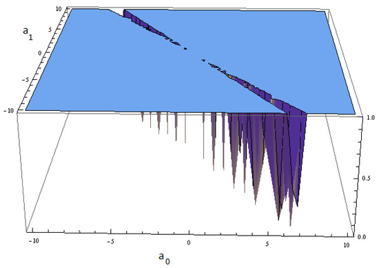
Figure 1. Stability region of $z=1$.

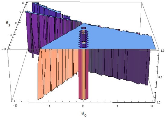
Figure 2. Stability region of $e{x}_1(a_0,a_1)$.

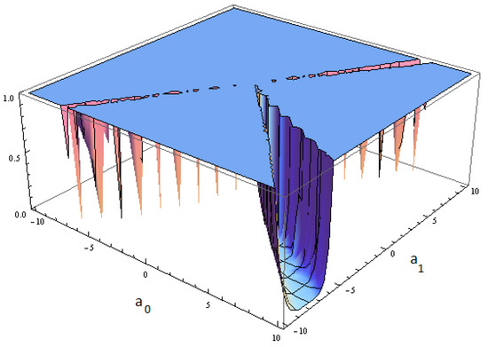
Figure 3. Stability region of $e{x}_2(a_0,a_1)$.

As a conclusion we can remark that the number and the stability of the fixed points depend on the parameters $a_0$ and $a_1$.

8.2. Study of the Critical Points and Parameter Spaces

In this section, we compute the critical points and we show the parameter spaces associated to the free critical points. It is well known that there is at least one critical point associated with each invariant Fatou component. The critical points of the family are the solutions of is $G^{\prime }(z,a_0,a_1)=0$, where

$$\begin{array}{c}{G}^{\prime }(z,a_0,a_1)=\hfill \\ \frac{2z^3{(1+z)}^2\left(6{\mathrm{a}0}^2+8\mathrm{a}0\mathrm{a}1+9{\mathrm{a}0}^{2}z+16\mathrm{a}0\mathrm{a}1z+12{\mathrm{a}1}^{2}z+6{\mathrm{a}0}^2{z}^2+8\mathrm{a}0\mathrm{a}1z^2\right)}{{\left(\mathrm{a}0+3\mathrm{a}0z+2\mathrm{a}1z+3\mathrm{a}0z^2+4\mathrm{a}1z^2\right)}^2}.\hfill \end{array}$$

By solving this equation, it is clear that $z=0$ and $z=\infty$ are critical points, which are related to the roots of the polynomial $p(z)$ and they have associated their own Fatou component. Moreover, there exist critical points no related to the roots, these points are called free critical points. Their expressions are:

$$c{r}_0=-1,$$

$$\begin{array}{c}c{r}_1(a_0,a_1)=\hfill \\ {\displaystyle \frac{-9{\mathrm{a}0}^2-16\mathrm{a}0\mathrm{a}1-12{\mathrm{a}1}^2-\sqrt{3}\sqrt{-21{\mathrm{a}0}^4-32{\mathrm{a}0}^3\mathrm{a}1+72{\mathrm{a}0}^2{\mathrm{a}1}^2+128\mathrm{a}0{\mathrm{a}1}^3+48{\mathrm{a}1}^4}}{4\left(3{\mathrm{a}0}^2+4\mathrm{a}0\mathrm{a}1\right)}}\hfill \end{array}$$

and

$$\begin{array}{c}c{r}_2(a_0,a_1)=\hfill \\ \frac{-9{\mathrm{a}0}^2-16\mathrm{a}0\mathrm{a}1-12{\mathrm{a}1}^2+\sqrt{3}\sqrt{-21{\mathrm{a}0}^4-32{\mathrm{a}0}^3\mathrm{a}1+72{\mathrm{a}0}^2{\mathrm{a}1}^2+128\mathrm{a}0{\mathrm{a}1}^3+48{\mathrm{a}1}^4}}{4\left(3{\mathrm{a}0}^2+4\mathrm{a}0\mathrm{a}1\right)}\hfill \end{array}$$

The relations between the free critical points are described in the following result.

Lemma 4.

(a) 

If$a_1=-\frac{a_0}{2}$or$a_1=\frac{a_0}{2}$

(i) $c{r}_1=c{r}_2=-1$.

(b) 

If$a_1=-\frac{3a_0}{2}$or$a_1=-\frac{7a_0}{6}$

(i) $c{r}_1=c{r}_2=1$.

(c) 

For other values of$a_0$and$a_1$

(i) The family has 3 free critical points.

Moreover, it is clear that for every value of$a_0$and$a_1$,$cr1(a_0,a_1)=\frac{1}{c{r}_2(a{0}_{,}{a}_1)}$

It is easy to see that $z=-1$ is a pre-periodic point as it is the pre-image of the fixed point related to the convergence to infinity, $z=1$, and the other free critical points are conjugated $c{r}_1(a_0,a_1)=1/c{r}_2(a_0,a_1)$. So, there are only two independent free critical points and only one is not pre-periodic. Without loss of generality, we consider in this paper the free critical point $c{r}_1(a_0,a_1)$. In order to find the best members of the family in terms of stability, the parameter space corresponding to this independent free critical point will be shown.

The study of the orbits of the critical points gives rise about the dynamical behavior of an iterative method. More precisely, to determinate if there exists any attracting extraneous fixed point or periodic orbit, the following question must be answered: For which values of the parameters, the orbits of the free critical points are attracting periodic orbits? In order to answer this question we are going to draw the parameter space but our main problem is that we have 2 free parameters $a_0$, $a_1$. In order to avoid this problem, we are going to use a a variant of the algorithm that appears in [43] and similar, in which we will consider the horizontal axis as the possible real values of $a_0$ and the vertical one as the possible values of $a_1$. When the critical point is used as an initial estimation, for each value of the parameter, the color of the point tell us about the place it has converged to: to a fixed point, to an attracting periodic orbit or even the infinity.

In Figure 4, the parameter space associated to $c{r}_1(a_0,a_1)$ is shown. The algorithm to draw this parameter speace is similar to the one used in [44]: A point is painted in cyan if considerint $z_0=c{r}_1(a_0,a_1)$ the iteration converges to 0 (which is related to one root), in magenta the convergence to ∞ (which is related to the other root) and in yellow appear the points which iteratations converges to 1 (which is related to ∞). Other colors used are:red for theconvergence to a extraneous fixed points and other colors, including black, for cycles.

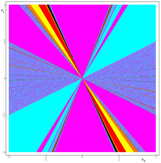
Figure 4. Parameter space associated to the free critical point $c{r}_1(a_0,a_1)$.

Now, we are going to show these anomalies using dynamical planes where the convergence to 0, after a maximum of 2000 iterations and with a tolerance of ${10}^{-6}$ appear in magenta, in cyan it appears the convergence to ∞, after a maximum of 2000 iterations and with a tolerance of ${10}^{-6}$ and in black the zones with no convergence to the roots. First of all, in Figure 5 and Figure 6 the dynamical planes associated with the values of $a_0$$a_1$ for which there is no convergence problems, are shown. As a consequence, those selections of pair of values are a good choice since all points converge to the roots of the original equation.

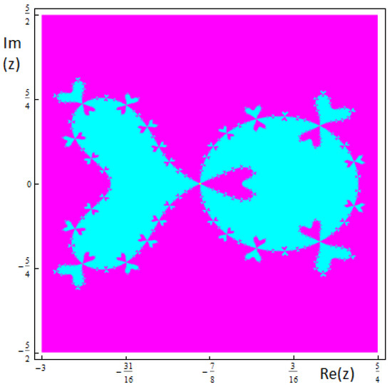
Figure 5. Basins of attraction associated to the member of the family $a_0=-5$ and $a_1=-4$.

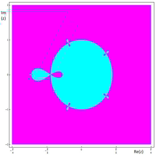
Figure 6. Basins of attraction associated to the member of the family $a_0=1$ and $a_1=-3/4$. This member has fifth order of convergence.

Then, focussing the attention in the region shown in Figure 4 it is evident that there exist members of the family with complicated behavior. In Figure 7, the dynamical planes of a member of the family with regions of convergence to any of the extraneous fixed points is shown. In this case, there exist regions of points which iterations do not converge to any of the roots of the original equations, so these values are not a good choice.

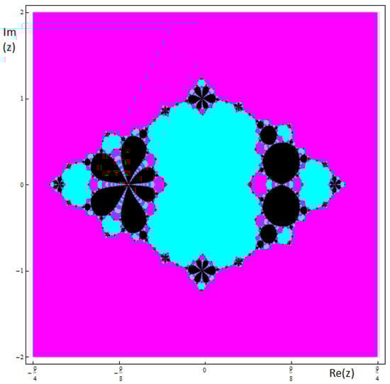
Figure 7. Basins of attraction associated to the member of the family $a_0=3.25$ and $a_1=-4.5$.

On the other hand, in Figure 4 and Figure 8, the dynamical planes of a member of the family with regions of convergence to $z=1$, related to ∞ is shown, in which we observe that there exist. In this case, there exist regions of points which iterations do not converge to any of the roots of the original equations, so these values are not a good choice.

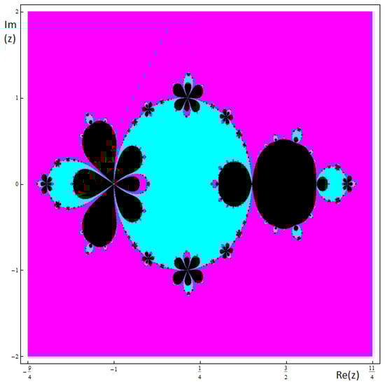
Figure 8. Basins of attraction associated to the member of the family $a_0=2.75$ and $a_1=-4.75$.

Finally, in Figure 9 and Figure 10, some dynamical planes of members of the family with convergence to different attracting cycles are shown.

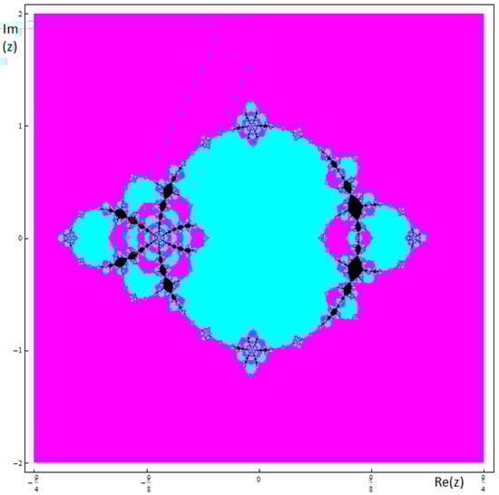
Figure 9. Basins of attraction associated to the member of the family $a_0=3.6$ and $a_1=-4.75$. The black zones are related to the convergence of a 2-cycle.

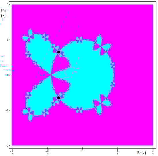
Figure 10. Basins of attraction associated to the member of the family $a_0=5$ and $a_1=0.1375$. The black zones in this case correspond with zones of convergence to a 3-cycle.

If we choose as a particular value of $a_0=5$ and $a_1=0.1375$ we can observe the existence of a periodic orbit of period 3

$$\{x_1=0.97769-0.210052i,x_2=0.75091-0.660405i,x_3=-0.763289-0.646058i\},$$

moreover, this orbit is attracting as

$$|G^{\prime }(x_1)G^{\prime }(x_2)G^{\prime }(x_3)|=0.265145\dots <1.$$

Sharkovsky’s Theorem [31], states that the existence of orbits of period 3, guaranties orbits of any period.

9. Conclusions

This article discusses purely iterative algorithms for Newton’s maps $T_f$, given by the Formula (1), and that were proposed in [6]. This family represents a large class of root finding algorithms, including the best known, and those of high order of convergence. Depending on the parameters $a_0$, $a_1$, $a_2$, $b_0$ and $b_1$, in general the family $T_f$ may not define a root finding algorithm. To avoid this difficulty, we achieved a characterization in terms of those parameters, so that it is effectively a root finding algorithm. The scaling theorem has the advantage of reducing the parameter space in dimension, and it is useful for plotting the parameter space in low dimension, among other things. We give a classification of extraneous fixed points and indifferent fixed points of $T_f$, in terms of the parameters $a_0$, $a_1$, $a_2$, $b_0$ and $b_1$. Then, we use those results and Hawkins’s theorem to conclude that over the family $T_f$, the rational map that generates generally convergent root finding algorithms, is the Halley’s method applied to cubic polynomials. This shows that rigidity is even stronger, and is not obtained only in terms of the conjugation.

References

- Hartman, P. Ordinary Differential Equations; John Wiley and Sons, Inc.: New York, NY, USA; London, UK; Sydney, Australia, 1964; p. xiv+612. [Google Scholar]
- Blanchard, P. The dynamics of Newton’s method, Complex dynamical systems. Proc. Symp. Appl. Math. Am. Math. Soc. 1994, 49, 139–154. [Google Scholar]
- Haeseler, F.V.; Peitgen, H.-O. Newton’s Method and Dynamical Systems; Peitgen, H.-O., Ed.; Kluwer Academic Publishers: Dordrecht, The Netherlands, 1989; pp. 3–58. [Google Scholar]
- McMullen, C. Families of rational maps and iterative root-finding algorithms. Ann. Math. 1987, 125, 467–493. [Google Scholar] [CrossRef]
- Hawkins, J. McMullen’s root-finding algorithm for cubic polynomials. Proc. Am. Math. Soc. 2002, 130, 2583–2592. [Google Scholar] [CrossRef]
- Honorato, G.; Plaza, S. Dynamical aspects of some convex acceleration methods as purely iterative algorithm for Newton’s maps. Appl. Math. Comput. 2015, 251, 507–520. [Google Scholar] [CrossRef]
- Arney, D.C.; Robinson, B.T. Exhibiting chaos and fractals with a microcomputer. Comput. Math. Appl. 1990, 19, 1–11. [Google Scholar] [CrossRef][Green Version]
- Buff, X.; Henriksen, C. König’s root-finding algorithms. Nonlinearity 2003, 16, 989–1015. [Google Scholar] [CrossRef]
- Crane, E. Mean value conjectures for rational maps. Complex Var. Elliptic Equ. 2006, 51, 41–550. [Google Scholar] [CrossRef]
- Curry, J.H.; Garnett, L.; Sullivan, D. On the iteration of a rational function: Computer experiment with Newton’s method. Commun. Math. Phys. 1983, 91, 267–277. [Google Scholar] [CrossRef]
- Drakopoulos, V. On the additional fixed points of Schröder iteration functions associated with a one–parameter family of cubic polynomials. Comput. Graph. 1998, 22, 629–634. [Google Scholar] [CrossRef]
- Honorato, G.; Plaza, S.; Romero, N. Dynamics of a higher-order family of iterative methods. J. Complex. 2011, 27, 221–229. [Google Scholar] [CrossRef]
- Kneisl, K. Julia sets for the super-Newton method, Cauchy’s method, and Halley’s method. Chaos 2001, 11, 359–370. [Google Scholar] [CrossRef] [PubMed]
- Rückert, J.; Schleicher, D. On Newton’s method for entire functions. J. Lond. Math. Soc. 2007, 75, 659–676. [Google Scholar] [CrossRef][Green Version]
- Sarría, Í.; González, R.; González-Castaño, A.; Magreñán, Á.A.; Orcos, L. A pedagogical tool based on the development of a computer application to improve learning in advanced mathematics. Rev. Esp. Pedagog. 2019, 77, 457–485. [Google Scholar]
- Vrscay, E. Julia sets and Mandelbrot–like sets associated with higher order Schröder rational iteration functions: A computer assisted study. Math. Comput. 1986, 46, 151–169. [Google Scholar]
- Blanchard, P. Complex Analytic Dynamics on the Riemann Sphere. Bull. AMS 1984, 11, 85–141. [Google Scholar] [CrossRef]
- Milnor, J. Dynamics in One Complex Variable: Introductory Lectures, 3rd ed.; Princeton U. Press: Princeton, NJ, USA, 2006. [Google Scholar]
- Smale, S. On the efficiency of algorithms of analysis. Bull. AMS 1985, 13, 87–121. [Google Scholar] [CrossRef]
- Amorós, C.; Argyros, I.K.; González, D.; Magreñán, A.A.; Regmi, S.; Sarría, Í. New improvement of the domain of parameters for newton’s method. Mathematics 2020, 8, 103. [Google Scholar] [CrossRef]
- Vrscay, E.; Gilbert, W. Extraneous fixed points, basin boundary and chaotic dynamics for Schröder and König rational iteration functions. Numer. Math. 1988, 52, 1–16. [Google Scholar] [CrossRef]
- Varona, J.L. Graphic and numerical comparison between iterative methods. Math. Intell. 2002, 24, 37–46. [Google Scholar] [CrossRef]
- Whittaker, E.T. A formula for the solution of algebraic and transcendental equations. Proc. Edinburgh Math. Soc. 1918, 36, 103–106. [Google Scholar] [CrossRef]
- Ezquerro, J.A.; Hernández, M.A. On a convex acceleration of Newton’s method. J. Optim. Theory Appl. 1999, 100, 311–326. [Google Scholar] [CrossRef]
- Schröder, E. On infinitely many algorithms for solving equations. Math. Annal. 1870, 2, 317–365. [Google Scholar] [CrossRef]
- Schröder, E. Ueber iterirte Functionen. Math. Ann. 1870, 3, 296–322. (In German) [Google Scholar] [CrossRef]
- Pomentale, T. A class of iterative methods for holomorphic functions. Numer. Math. 1971, 18, 193–203. [Google Scholar] [CrossRef]
- Gilbert, W.J. Newton’s method for multiple roots. Comput. Graph. 1994, 18, 227–229. [Google Scholar] [CrossRef]
- Gutiérrez, J.M.; Hernández, M.A. An acceleration of Newton’s method: Super-Halley method. Appl. Math. Comput. 2001, 117, 223–239. [Google Scholar] [CrossRef]
- Gutiérrez, J.M.; Hernández, M.A. A family of Chebyshev-Halley type methods in Banach spaces. Bull. Aust. Math. Soc. 1997, 55, 113–130. [Google Scholar] [CrossRef]
- Cordero, A.; Torregrosa, J.R.; Vindel, P. Dynamics of a family of Chebyshev Halley type methods. Appl. Math. Comput. 2013, 219, 8568–8583. [Google Scholar] [CrossRef]
- Amat, S.; Busquier, S.; Plaza, S. Review of some iterative root-finding methods from a dynamical point of view. Sci. Ser. A Math. Sci. 2004, 10, 3–35. [Google Scholar]
- Amat, S.; Busquier, S.; Gutiérrez, J.M. Geometric constructions of iterative functions to solve nonlinear equations. J. Comput. Appl. Math. 2003, 157, 197–205. [Google Scholar] [CrossRef]
- Amorós, C.; Argyros, I.K.; Magreñán, Á.A.; Regmi, S.; González, R.; Sicilia, J.A. Extending the applicability of Stirling’s method. Mathematics 2020, 8, 35. [Google Scholar] [CrossRef]
- Argyros, I.K.; Chen, D. Results on the Chebyshev method in Banach spaces. Proyecciones 1993, 12, 119–128. [Google Scholar] [CrossRef]
- Drakopoulos, V.; Argyropoulos, N.; Böhm, A. Generalized computation of Schröder iteration functions to motivated families of Julia and Mandelbrot–like sets. SIAM J. Numer. Anal. 1999, 36, 417–435. [Google Scholar] [CrossRef]
- Hernández, M.A.; Salanova, M.A. A family of Chebyshev-Halley type methods. Int. J. Comput. Math. 1993, 47, 59–63. [Google Scholar] [CrossRef]
- Moysi, A.; Argyros, I.K.; Regmi, S.; González, D.; Magreñán, Á.A.; Sicilia, J.A. Convergence and dynamics of a higher-order method. Symmetry 2020, 12, 420. [Google Scholar] [CrossRef]
- Plaza, S. Conjugacy classes of some numerical methods. Proyecciones 2001, 20, 1–17. [Google Scholar] [CrossRef]
- Argyros, I.K.; Magreñán, Á.A. Iterative Methods and Their Dynamics with Applications: A Contemporary Study; CRC Press: Boca Raton, FL, USA; Taylor & Francis Group: Boca Raton, FL, USA, 2017. [Google Scholar]
- Magreñán, Á.A.; Argyros, I.K. A Contemporary Study of Iterative Methods: Convergence, Dynamics and Applications; Elsevier: Amsterdam, The Netherlands, 2017. [Google Scholar]
- Magrenán, Á.A. Different anomalies in a Jarratt family of iterative root-finding methods. Appl. Math. Comput. 2014, 233, 29–38. [Google Scholar]
- Magreñán, Á.A. A new tool to study real and complex dynamics: The convergence plane. Appl. Math. Comput. 2014, 248, 215–224. [Google Scholar]
- Amat, S.; Argyros, I.K.; Busquier, S.; Magreñán, Á.A. Local convergence and the dynamics of a two-point four parameter Jarratt-like method under weak conditions. Numer. Algorithms 2017, 74, 371–391. [Google Scholar] [CrossRef]
© 2020 by the authors. Licensee MDPI, Basel, Switzerland. This article is an open access article distributed under the terms and conditions of the Creative Commons Attribution (CC BY) license (http://creativecommons.org/licenses/by/4.0/).