On the Dual and Inverse Problems of Scheduling Jobs to Minimize the Maximum Penalty

Abstract

In this paper, we consider the single-machine scheduling problem with given release dates and the objective to minimize the maximum penalty which is NP-hard in the strong sense. For this problem, we introduce a dual and an inverse problem and show that both these problems can be solved in polynomial time. Since the dual problem gives a lower bound on the optimal objective function value of the original problem, we use the optimal function value of a sub-problem of the dual problem in a branch and bound algorithm for the original single-machine scheduling problem. We present some initial computational results for instances with up to 20 jobs.

1. Introduction

We consider single-machine scheduling problems, where a set of n jobs $N=\{1,2,\dots ,n\}$ has to be processed on a single machine starting at time $\tau$. For each job j, a release date $r_j$, a processing time $p_j$ and a due date $d_j$ are given. Many scheduling problems require the minimization of some maximum term. Denote by $C_j$ the completion time of job j, then the minimization of the makespan (i.e., the maximum completion time of the jobs)

$$C_{max}=\underset{j=1,\dots ,n}{max}{C}_j,$$

or the minimization of maximum lateness

$$L_{max}=\underset{j=1,\dots ,n}{\max }\{C_j-d_j\}$$

are well-known examples of such an optimization criterion.

In this paper, we consider two related problems of such a min-max problem, namely a dual problem as well as an inverse problem of the single-machine scheduling problem with given release dates and minimizing the maximum penalty. While the original problem $1|r_j|L_{max}$ is $NP$-hard in the strong sense [1], we prove that both the dual and inverse problems of this problem can be solved in polynomial time.

Due to the $NP$-hardness of the problem $1|r_j|L_{max}$, several branch and bound algorithms have been developed and special cases of the problem have been considered, see e.g., [2,3,4,5,6,7,8,9]. In [9], it has been shown that if the release dates for all jobs are from the interval $[d_j-p_j-A,d_j-A]$ for all jobs and some constant A, the problem can be solved in $O\left(n\log n\right)$ time if no machine idle times are allowed and in $O\left(n^2\log n\right)$ time if machine idle times are allowed. Another important special case of this problem has been considered in [10]. In that paper, it is shown that for naturally bounded job data, the problem can be polynomially solved. More precisely, a polynomial time solution of the variant is given when the maximal job processing time and the differences between the job release dates are bounded by a constant. The binary search procedure presented in this work determines an optimal solution in $O\left(n^2\log n\log p_{max}\right)$ or $O\left(d_{max}n\log n\log p_{max}\right)$ time, where $p_{max}$ is the maximal processing time and $d_{max}$ is the maximal due date.

In [11], some computational experiences and applications for the more general case with additional precedence constraints are reported. Their algorithm turned out to be superior to earlier algorithms. Some applications to job shop scheduling are also discussed. A more recent branch and bound algorithm for this single-machine problem with release dates and precedence constraints has been given in [12]. This algorithm uses four heuristics for finding initial upper bounds and a variable neighborhood search procedure. It solved most considered instances within one minute of CPU time. Several approximation schemes for four variants of the problem with additional non-availability or deadline constraints have been derived in [13]. An approximation algorithm for this single-machine problem with additional workload dependent maintenance duration has been presented in [14]. This algorithm is even optimal for some special cases of the problem. A hybrid metaheuristic search algorithm for the single-machine problem with given release dates and precedence constraints has been developed in [15]. Computational tests have been made using own instance sets with 100 jobs and instances from [12] with up to 1000 jobs. The hybridization of the elektromagnetism algorithm with tabu search leads to a tradeoff between diversification and intensification strategies. The metric approach is another recent possibility for solving the problem $1|r_j|L_{max}$ approximately with guaranteed maximal error, see e.g., [16]. The introduced metric delivers an upper bound on the absolute error of the objective function value. Taking a given instance of some problem and using the introduced metric, the nearest instance is determined for which a polynomial or pseudo-polynomial algorithm is known. Then a schedule is constructed for this instance and applied to the original instance.

There have been also considered problems with several optimization criteria. In [17], the single-machine problem with the primary criterion of minimizing maximum lateness and the secondary criterion of minimizing the maximum job completion time has been investigated. The author gives dominance properties and conditions when the Pareto-optimal set can be found in polynomial time. The derived properties allow extension of the basic framework to exponential implicit enumeration schemes and polynomial approximation algorithms. The problem of finding the Pareto-optimal set for two criteria in the case when there are constraints on the source data have been considered in [18,19]. In [18], the idea of the dual approach is considered in detail, but there is no sufficient experimental study of the effectiveness of this approach. Lazarev et al. [20] considered the problem of minimizing maximum lateness and the makespan in the case of equal processing times and proposed a polynomial time approach for finding the Pareto-optimal set of feasible solutions. They presented two approaches, the efficiency of which depends on the number of jobs and the accuracy of the input-output parameters.

The dual and inverse problems considered in this paper are maximization problems. In the literature, there exist some works on other single-machine maximization problems, usually under the assumption of no inserted idle times between the processing of jobs on the machine. Maximization problems in single-machine problems were considered e.g., in [21,22]. The complexity and some algorithms for single-machine total tardiness maximization problems have been discussed in [23]. In [24], a pseudo-polynomial algorithm for the single-machine total tardiness maximization problem has been transformed by a graphical algorithm into a polynomial one.

The remainder of this paper is as follows. In Section 2, we introduce the dual problem of the single-machine problem, where the maximum penalty term of a job should be minimized. Section 3 considers an inverse problem, where the minimum of the penalty terms should be maximized. The solution of this dual problem is embedded into a branch and bound algorithm for the original problem. Some computational results for this branch and bound algorithm are given in Section 4. The paper finishes with some concluding remarks.

2. The Dual Problem

Let us consider the general formulation of the $NP$-hard problem of minimizing the maximum penalty or cost ${\phi }_{\max }$ for a set of jobs on a single machine, i.e., problem $1\mid r_j\mid {\phi }_{\max }$. The machine cannot process more than one job of the set $N=\{1,\dots ,n\}$ at a moment. Preemptions of the processing of a job are prohibited. Let ${\phi }_{j_k}\left(C_{j_k}\left(\pi \right)\right)$ denote the penalty for job $j\in N$ if it is processed as the k-th job in the sequence $\pi =(j_1,j_2,\dots ,j_k,\dots ,j_n)$. We assume that all ${\phi }_{j_k}\left(C_{j_k}\left(\pi \right)\right),k=1,2,\dots ,n,$ are arbitrary non-decreasing penalty functions.

By ${\mu }^{*}$ we denote the optimal value of the objective function:

$${\mu }^{*}=\underset{\pi \in \Pi \left(N\right)}{\min }\underset{k=1,\dots ,n}{\max }{\phi }_{j_k}\left(C_{j_k}\left(\pi \right)\right),$$

(1)

where $\Pi \left(N\right)=\{{\pi }_1,{\pi }_2,\dots ,{\pi }_{n!}\}$ denotes the set of all permutations (schedules) of the jobs of the set N.

In the scheduling literature, many special cases of the following general dual problem are considered. One wishes to find an optimal job sequence ${\pi }^{*}$ and the corresponding objective function value ${\nu }^{*}$ such that

$${\nu }^{*}=\underset{k=1,\dots ,n}{\max }\underset{\pi \in \Pi \left(N\right)}{\min }{\phi }_{j_k}\left(C_{j_k}\left(\pi \right)\right).$$

(2)

For convenience, we introduce a notation that takes into account the position of the job in the schedule. Let a schedule (job sequence) $\pi \in \Pi \left(N\right)$ be given by $\pi =(j_1,j_2,\cdots ,j_n)$. For the job, which is processed as the k-th job in the sequence, $k=1,2,\cdots ,n,$ under a schedule $\pi$, we denote:

$${\nu }_k=\underset{\pi \in \Pi \left(N\right)}{\min }{\phi }_{j_k}\left(C_{j_k}\left(\pi \right)\right),k=1,2,\cdots ,n.$$

(3)

Obviously,

$${\nu }^{*}=\underset{k=1,\dots ,n}{\max }{\nu }_k.$$

(4)

Lemma 1

([25]). Let ${\phi }_j\left(t\right),j=1,2,\cdots ,n,$ be arbitrary non-decreasing penalty functions in the problem $1\mid r_j\mid {\phi }_{\max }$. Then we have ${\nu }_n\ge {\nu }_k$ for all $k=1,2,\cdots ,n$, i.e., ${\nu }^{*}={\nu }_n.$

Proof. 

Suppose that there exists a number $k,$$k<n,$ such that ${\nu }_k>{\nu }_n$. Assume that ${\pi }_n=(j_1,j_2,\cdots ,j_n)$ is a schedule for which the value ${\nu }_n$ is obtained. Then we consider the schedule

$$\pi =(j_{n-k+1},j_{n-k+2},\cdots ,j_n,j_1,j_2,\cdots ,j_{n-k}).$$

Please note that under the schedule $\pi$, the job $j_n$ will be carried out as the k-th job in the sequence. Since $C_{j_n}\left({\pi }_n\right)\ge C_{j_n}\left(\pi \right)$, we have

$${\nu }_n={\phi }_{j_n}\left(C_{j_n}\left({\pi }_n\right)\right)\ge {\phi }_{j_n}\left(C_{j_n}\left(\pi \right)\right)\ge {\nu }_k.$$

Due to the assumption ${\nu }_k>{\nu }_n$, we obtain the inequality

$${\nu }_k>{\nu }_n\ge {\nu }_k$$

which is a contradiction. The lemma has been proved.  □

Thus, the solution of the dual problem $1|r_j|{\varphi }_{max}$ is reduced to the problem of finding the value ${\nu }_n$. We enumerate all jobs in order of non-decreasing release dates: $r_{i_1}\le r_{i_2}\le \cdots \le r_{i_n}$. Due to

$${\nu }_n=\underset{\pi \in \Pi \left(N\right)}{\min }{\phi }_{j_n}\left(C_{j_n}\left(\pi \right)\right),$$

we will put each of the jobs j of the set N onto the last (i.e., the n-th) position. The other $n-1$ jobs of the set $N\backslash \left\{j\right\}$ are arranged in their original order starting at time $\tau$. This gives the earliest completion time of processing the jobs from the set $N\backslash \left\{j\right\}$. This procedure is formally summarized in Algorithm 1. The input data of Algorithm 1 is the pair $(N,\tau )$, where $\tau$ is used to calculate $C_j$.

Algorithm 1: Solution of the dual problem of the problem $1\mid r_j\mid {\phi }_{\max }$

Construct the schedule ${\pi }^r=(i_1,i_2,\dots ,i_n)$, in which all jobs are sequenced according to non-decreasing release dates: $r_{i_1}\le r_{i_2}\le \dots \le r_{i_n}$. For $k=1,2,\dots ,n,$ find the value ${\phi }_{i_k}\left(C_{i_k}\left({\pi }_k\right)\right)$ for the schedule ${\pi }_k=({\pi }^r\backslash i_k,i_k).$ Find the value ${\nu }^{*}=\underset{k=1,\dots ,n}{\min }{\phi }_{i_k}\left(C_{i_k}\left({\pi }_k\right)\right)$ and the job $i_k$, which gives the value ${\nu }^{*}$.

The complexity of Algorithm 1 can be estimated as follows. We need $O\left(n\log n\right)$ operations to construct the schedule ${\pi }^r$. We need $O\left(n\right)$ operations to find each of the n values ${\phi }_{i_k}\left(C_{i_k}\left({\pi }_k\right)\right)$. Therefore, to determine the value ${\nu }^{*}$ and the corresponding job $i_k$, for which the value ${\nu }^{*}$ is obtained, no more than $O\left(n^2\right)$ operations are required.

Theorem 1

([25]). Let ${\phi }_j\left(t\right),j=1,2,\cdots ,n,$ be arbitrary non-decreasing penalty functions for the problem $1\mid r_j\mid {\phi }_{\max }$. Then the inequality ${\mu }^{*}\ge {\nu }^{*}$ holds.

Proof. 

Suppose the opposite, i.e., there exists an instance of the problem $1\mid r_j\mid {\phi }_{\max }$, for which the inequality ${\mu }^{*}<{\nu }^{*}$ holds. Let ${\pi }^{*}=(j_1,j_2,\cdots ,j_n)$ be an optimal schedule for this instance. Then we have

$${\phi }_{j_n}\left(C_{j_n}\left({\pi }^{*}\right)\right)\le {\mu }^{*}<{\nu }^{*},$$

which contradicts equality (3):

$${\nu }^{*}={\nu }_n=\underset{\pi \in \Pi \left(N\right)}{\min }{\phi }_{j_n}\left(C_{j_n}\left(\pi \right)\right).$$

The theorem has been proved.  □

The obtained estimate can be efficiently used in constructing schemes of a branch and bound method for solving the problem $1\mid r_j\mid {\phi }_{max}$, and for estimating the error of approximate solutions when the branch and bound algorithm stops without finding an optimal solution.

We denote by $\{N^{\prime },{\tau }^{\prime },{\nu }^{\prime },{\pi }^{\prime },B^{\prime }\}$ the sub-problem of processing the jobs of the set $N^{\prime }\subseteq N$ from time ${\tau }^{\prime }\ge \tau$ on according to some partial sequence ${\pi }^{\prime }$ for the jobs of the set $N\backslash N^{\prime }$, where ${\nu }^{\prime }$ is the lower bound obtained by solving the dual problem of this instance, ${\tau }^{\prime }=C_{\max }({\pi }^{\prime },\tau )$ is the start time of the planning horizon for the jobs from the set $B^{\prime }$, which is equal to the makespan value for the sequence ${\pi }^{\prime }$, and $\tau$ is the time when the machine is ready to process the jobs from the set N. $B^{\prime }$ is the set of jobs that cannot be placed on the corresponding first position of the schedule.

The subsequent Algorithm 2 implements one of the possible schemes of the branch and bound method using the solution of the dual problem. The branching in Algorithm 2 is carried out as a result of dividing the current sub-instance into two instances: put the job f (the job with the smallest due date from the set of jobs ready for processing) at the next position in the schedule and prohibit the inclusion of the job f at the next position in the schedule (by increasing the possible start time of job f).

Denote

$$r_j\left(\tau \right)=\max \{r_j,\tau \},r(N,\tau )=\underset{j\in N}{\min }{r}_j\left(\tau \right).$$

Let $\left|N\right|>1$. We choose a job $f=f(N,\tau )$ from the set N such that

$$f(N,\tau )=\arg \underset{j\in N\backslash B}{\min }\left\{d_j\mid r_j\left(\tau \right)=r(N,\tau )\right\}.$$

If $N=\left\{i\right\}$, then $f(N,\tau )=i$ for all $\tau$. Here B is a set of jobs that cannot be placed on the current first position. Denote by ${\pi }^{*}$ the currently best schedule constructed for all jobs.

We note that a deeper comparative discussion of the characteristics of the particular search strategies can be found in [26,27].

Algorithm 2: Solution of the problem $1\mid r_j\mid L_{\max }$ by the branch and bound method based on the solution of the dual problem

1. Initial step Let ${\pi }^{*}=\varnothing$. The list of instances contains the original instance $\{N,\tau ,\nu ,\varnothing ,\varnothing \}$, where $\nu$ is a lower bound on the optimal objective function value obtained by solving the dual problem of this instance.  2. Main step (a) From the list of instances, select an instance $\{N^{\prime },{\tau }^{\prime },{\nu }^{\prime },{\pi }^{\prime },B^{\prime }\}$ with a minimal lower bound ${\nu }^{\prime }$. (b) Find the job $f=f(N^{\prime },{\tau }^{\prime })$ from the set $N^{\prime }\backslash B^{\prime }$ with the smallest due date from the number of jobs ready for processing at time ${\tau }^{\prime }$. (c) Replace the instance $\{N^{\prime },{\tau }^{\prime },{\nu }^{\prime },{\pi }^{\prime },B^{\prime }\}$ by the two instances $\{N_1,{\tau }_1,{\nu }_1,{\pi }_1,B_1\}$ and $\{N_2,{\tau }_2,{\nu }_2,{\pi }_2,B_2\}$ in the list of instances, where: - $N_1=N^{\prime }\backslash \left\{f\right\},{\tau }_1=max\{r_f,{\tau }^{\prime }\}+p_f,B_1=\varnothing ,{\pi }_1=({\pi }^{\prime },f),{\nu }_1$ is a lower bound obtained by solving the dual problem of this instance by Algorithm 3; - $N_2=N^{\prime },{\tau }_2={\tau }^{\prime },B_2=B^{\prime }\cup \left\{f\right\},{\pi }_2={\pi }^{\prime },{\nu }_2$ is a lower bound obtained by solving the dual problem of this instance by Algorithm 3. (d) If, after completing this step of the algorithm, we obtain $\left\{{\pi }_1\right\}=N$, that is, all jobs are ordered, then ${\pi }^{*}=argmin\{L_{max}({\pi }_1,\tau ),L_{max}({\pi }^{*},\tau )\}$. (e) Exclude all instances $\{N^{\prime },{\tau }^{\prime },{\nu }^{\prime },{\pi }^{\prime },B^{\prime }\}$, for which ${\nu }^{\prime }\ge L_{max}({\pi }^{*},\tau )$.  3. Termination step If the list of instances is empty, STOP, otherwise repeat the main step 2.

To find the value $\nu$ in step 2(c), we need to modify Algorithm 1 taking into account a list B of jobs that cannot be placed on the current position. The input data of Algorithm 3 is the triplet $(N,\tau ,B)$, where $\tau$ is used to calculate $C_j$.

Algorithm 3: Modification of the solution algorithm for the dual problem of the problem $1\mid r_j\mid {\phi }_{max}$ with respect to a list of jobs that cannot be on the first position

Construct the schedule ${\pi }^r=(i_1,i_2,\cdots ,i_n)$, in which all jobs are sequenced according to non-decreasing release dates: $r_{i_1}\le r_{i_2}\le \dots \le r_{i_n}$. For $k=1,2,\cdots ,n,$ if $N\backslash (B\cup \left\{i_k\right\})\ne \varnothing$, find a job $$i_l=\arg \underset{j\in N\backslash (B\cup \left\{i_k\right\})}{\min }{r}_j$$ and construct the schedule ${\pi }_k=(i_l,{\pi }^r\backslash \{i_l,i_k\},i_k)$. Find the value ${\phi }_{i_k}\left(C_{i_k}\left({\pi }_k\right)\right)$. If $N\backslash (B\cup \left\{i_k\right\})=\varnothing$, then we assume $C_{i_k}=+\infty$. Find the value ${\nu }^{*}=\underset{k=1,\dots ,n}{\min }{\phi }_{i_k}\left(C_{i_k}\left({\pi }_k\right)\right)$ and the job $i_k$, which gives the value ${\nu }^{*}$.

It is easy to see that this algorithm can be used to solve the more general problem $1\mid r_j\mid {\phi }_{\max }$. In addition, if the algorithm is stopped without an empty list of instances due to a time limit, the current schedule ${\pi }^{*}$ can be taken as an approximate solution of the problem.

Hence, although the original problem $1\mid r_j\mid {\phi }_{\max }$ is $NP$-hard in the strong sense (recall that problem $1\mid r_j\mid L_{\max }$ is $NP$–hard in the strong sense), the dual problem turned out to be polynomially solvable.

If precedence relations are specified between the jobs by an acyclic graph G, then the dual problem of the problem $1\mid r_j,prec\mid {\phi }_{\max }$ can also be solved in a similar way. Since the argumentation is similar, we skip the details. Here, the core is to solve the problem $1\mid r_j,prec\mid C_{\max }$. Jobs without successors according to the precedence graph G will be put one-by-one to the last positions in the job sequence. Thus, the dual problem of the problem $1\mid r_j,prec\mid {\phi }_{\max }$ is also polynomially solvable.

For problems with $m>1$ machines, e.g., problem $Pm\mid r_j,prec\mid {\phi }_{\max }$, the core consists of solving the dual problem, which is the partition problem. This dual problem is $NP$–hard in the ordinary sense.

Thus, although in mathematical programming the original and dual problems have usually the same complexity status, it turned out that the dual problems of the scheduling problems considered in this paper have a lower complexity than the original problems. This interesting fact should be investigated further in more detail also for other scheduling problems.

3. The Inverse Problem of the Maximum Lateness Problem

The inverse problem of the $NP$-hard problem of minimizing maximum lateness $1\mid r_j\mid L_{\max }$ consists of finding a schedule $\pi$, which reaches the maximum minimal lateness and finding the value

$${\lambda }^{*}=\underset{\pi \in \Pi \left(N\right)}{\max }\underset{k=1,\dots ,n}{\min }{L}_{j_k}\left(C_{j_k}\left(\pi \right)\right).$$

(5)

Please note that for this problem, inserted idle times of the machine are prohibited.

This problem was solved only for the case of simultaneous availability of the set N for processing, i.e., $r_j=0$, for all $j\in N$ in [28]. We consider the general case of the problem $1\mid r_j\mid \max L_{\min }$.

Lemma 2.

There exists an optimal schedule $\pi =(i_1,\cdots ,i_n)$ for the problem $1\mid r_j\mid \max L_{\min }$, for which

$$d_{i_k}-p_{i_k}\le d_{i_{k+1}}-p_{i_{k+1}},k=2,3,\cdots ,n-1,$$

(6)

and

$${\lambda }^{*}=\underset{k=1,\dots ,n}{\min }{L}_{i_k}\left(C_{i_k}\left(\pi \right)\right).$$

Proof. 

Assume that at least one of inequalities (6) is not satisfied for an optimal schedule ${\pi }^{\prime }=(j_1,\cdots ,j_n)$ and let

$${\lambda }^{*}=\underset{k=1,\dots ,n}{\min }{L}_{i_k}\left(C_{i_k}\left({\pi }^{\prime }\right)\right).$$

In what follows, the proof will consist of two stages, which can be repeated several times.

Step 1. If there are no machine idle times in the schedule ${\pi }^{\prime }$, then go to step 2. Let there be idle times according to schedule ${\pi }^{\prime }$, and consider the last of them:

$$C_{j_k}<r_{j_{k+1}}and{r}_{j_m}\le C_{j_{m-1}},m=k+2,\cdots ,n.$$

Construct the schedule ${\pi }^{″}=(j_{k+1},j_1,\cdots ,j_k,j_{k+2},\cdots ,j_n)$. Since

$$C_j\left({\pi }^{″}\right)\ge C_j\left({\pi }^{\prime }\right)\mathrm{for}\mathrm{all}j\in N,$$

the value of the minimal lateness will not decrease. There will be no idle time under the schedule ${\pi }^{″}$, and the optimal value ${\lambda }^{*}$ will be saved. Set ${\pi }^{\prime }:={\pi }^{″}$ and go to step 2.

Step 2. If the schedule ${\pi }^{\prime }$ meets the conditions of Lemma 2, the proof is completed. If there exist two jobs $j_l,j_{l+1}$, for which

$$d_{j_l}-p_{j_l}>d_{j_{l+1}}-p_{j_{l+1}},$$

then exchange the jobs $j_l,j_{l+1}$ which yields the schedule

$${\pi }^{″}=(j_1,\cdots ,j_{l-1},j_{l+1},j_l,j_{l+2},\cdots ,j_n).$$

As there are no machine idle times under the schedule ${\pi }^{\prime }$, we have

$$r_{j_l}\le C_{j_{l-1}}\left({\pi }^{\prime }\right).$$

There are the following possible cases:

(1) Let $r_{j_{l+1}}\le C_{j_{l-1}}\left({\pi }^{\prime }\right)$. Obviously, in this case we have

$$C_{j_k}\left({\pi }^{\prime }\right)=C_{j_k}\left({\pi }^{″}\right),k=1,2,\cdots ,l-1,l+2,\cdots ,n.$$

(7)

According to the assumptions, inequality

$$C_{j_{l-1}}\left({\pi }^{\prime }\right)+p_{j_l}+p_{j_{l+1}}-d_{j_{l+1}}>C_{j_{l-1}}\left({\pi }^{\prime }\right)+p_{j_l}-d_{j_l}.$$

(8)

holds. Moreover, we have

$$C_{j_{l-1}}\left({\pi }^{\prime }\right)+p_{j_{l+1}}-d_{j_{l+1}}>C_{j_{l-1}}\left({\pi }^{\prime }\right)+p_{j_l}-d_{j_l};$$

(9)

$$C_{j_{l-1}}\left({\pi }^{\prime }\right)+p_{j_{l+1}}-d_{j_l}>C_{j_{l-1}}\left({\pi }^{\prime }\right)+p_{j_l}-d_{j_l}.$$

(10)

Formulas (7)–(10) show that the maximal lateness is not reduced. Set ${\pi }^{\prime }:={\pi }^{″}$ and repeat step 2.

(2) Let $r_{j_{l+1}}>C_{j_{l-1}}\left({\pi }^{\prime }\right)$. In this case, we have

$$C_{j_k}\left({\pi }^{″}\right)=C_{j_k}\left({\pi }^{\prime }\right),k=1,2,\cdots ,l-1,$$

(11)

$$C_{j_k}\left({\pi }^{″}\right)>C_{j_k}\left({\pi }^{\prime }\right),k=l+2,\cdots ,n.$$

(12)

According to the assumptions, we have

$$C_{j_{l+1}}\left({\pi }^{″}\right)-d_{j_{l+1}}>C_{j_l}\left({\pi }^{\prime }\right)-d_{j_l};$$

(13)

$$C_{j_l}\left({\pi }^{″}\right)-d_{j_l}>C_{j_{l+1}}\left({\pi }^{\prime }\right)-d_{j_{l+1}}.$$

(14)

Formulas (8) and (11)–(14) show that the maximal lateness is not reduced. Set ${\pi }^{\prime }:={\pi }^{″}$ and go to step 1.

In a finite number of steps, we construct an optimal schedule satisfying the conditions of the lemma. The lemma has been proved.  □

Algorithm 4 constructs n schedules, one of which is satisfying the conditions of the lemma.

Algorithm 4: Solution of the inverse problem $1\mid r_j\mid max{L}_{min}$

1. Enumerate all jobs of the set N according to $d_1-p_1\le d_2-p_2\le \dots \le d_n-p_n$. 2. For $k=1,2,\dots ,n$ do: (a) construct the schedule ${\pi }_k=(k,1,\dots ,k-1,k+1,\dots ,n)$ and (b) determine ${\lambda }_k=\underset{j=1,\dots ,n}{\min }{L}_j\left(C_j\left({\pi }_k\right)\right)$. 3. Calculate ${\lambda }^{*}=\underset{k=1,\dots ,n}{\max }{\lambda }_k$.

$O\left(n\log n\right)$ operations are needed for renumbering the jobs of the set N. $O\left(n\right)$ operations are needed for constructing the schedule ${\pi }_k$ and calculating the value ${\lambda }_k,$$k=1,\dots ,n$. Thus, no more than $O\left(n^2\right)$ operations are needed to find the value ${\lambda }^{*}$.

The objective function value of a solution of the problem of maximizing minimal lateness $1\mid r_j\mid \max L_{\min }$ is a lower bound on the optimal objective function value for the original problem $1\mid r_j\mid L_{\max }$.

Theorem 2

([18]). For the optimal function values of the problem $1\mid r_j\mid L_{\max }$ and the corresponding inverse problem $1\mid r_j\mid \max L_{\min }$, the inequality ${\mu }^{*}\ge {\lambda }^{*}$ holds.

Proof. 

Denote by ${\pi }^{\prime }$ and ${\pi }^{″}$ optimal schedules for the problems $1\mid r_j\mid L_{\max }$ and $1\mid r_j\mid \max L_{\min }$, respectively. There exist jobs $k^{\prime },k^{″}\in N$, for which the following inequalities hold:

$${\mu }^{*}=C_{k^{\prime }}\left({\pi }^{\prime }\right)-d_{k^{\prime }}\ge C_j\left({\pi }^{\prime }\right)-d_j\mathrm{for}\mathrm{all}j\in N;$$

(15)

$$C_j\left({\pi }^{″}\right)-d_j\ge C_{k^{″}}\left({\pi }^{″}\right)-d_{k^{″}}={\lambda }^{*}\mathrm{for}\mathrm{all}j\in N.$$

(16)

Please note that jobs $k^{\prime }$ and $k^{″}$ can be identical. Let ${\pi }^{″}=(j_1,\cdots ,j_n)$. Obviously, the following inequality is satisfied for job $j_1$:

$$C_{j_1}\left({\pi }^{\prime }\right)-d_{j_1}\ge C_{j_1}\left({\pi }^{″}\right)-d_{j_1}.$$

(17)

According to inequalities (15)–(17), we get

$${\mu }^{*}=C_{k^{\prime }}\left({\pi }^{\prime }\right)-d_{k^{\prime }}\ge C_{j_1}\left({\pi }^{\prime }\right)-d_{j_1}\ge C_{j_1}\left({\pi }^{″}\right)-d_{j_1}\ge C_{k^{″}}\left({\pi }^{″}\right)-d_{k^{″}}={\lambda }^{*},$$

i.e., ${\mu }^{*}\ge {\lambda }^{*}.$ The theorem has been proved.  □

4. Computational Results

In this section, we present some results of the numerical experiments carried out on randomly generated test instances. The numerical experiments were carried out on a PC Intel® Core™ i5-4210U CPU @ 1.70GHz, 4 cores; 8 GB DDR4 RAM.

Various methods of generating test instances for different types of scheduling problems are described in [29]. For the problem $1|r_j|L_{max}$ with n jobs, the authors suggest the following generation scheme:

• $r_0=0$ and $r_i=r_{i-1}+X_i$, where $X_i\sim \exp \left(\lambda \right)$, for $i=1,\dots ,n$;
• $p_i\sim N(\mu ,\sigma )$ for $i=1,\dots ,n$, truncated below a known lower bound;
• $d_i=r_i+kE\left[p_i\right]$ for $i=1,\dots ,n$, where $k\ge 1$.

The authors suggest that $\lambda ,\mu ,\sigma$ and k are generation parameters that can be fixed by the user. Applying this generation scheme, we generate release dates which are independent from the processing times, while the due dates correlate with the processing times, as it usually happens in real problems. We set

$$\lambda =\frac{1}{100},\mu =100,\sigma =40,k=1$$

and generated 15 instances for each $n\in \{3,4,\dots ,20\}$. The results are shown in

Table 1. Number of branching points in Algorithm 2 for the test instances generated according to [29].

n	Number of the Instance
	1	2	3	4	5	6	7	8	9	10	11	12	13	14	15
3	4	2	2	2	2	2	2	2	2	2	2	4	2	2	2
4	3	3	3	3	3	3	3	3	3	5	4	3	3	3	3
5	9	4	4	25	4	4	31	4	4	8	4	4	4	4	18
6	5	5	64	227	161	13	7	5	5	5	5	5	84	15	5
7	6	25	16	6	6	6	31	147	310	34	35	6	172	6	222
8	7	234	33	7	7	23	7	391	7	7	7	7	194	7	7
9	1271	8	1847	8	3786	2934	8	8	62	8	8	721	8	208	8
10	9	690	9	9	66	114	9	9	9	9	9	9	3944	6584	9
11	10	13,098	10	5071	10	13,992	11	10	6081	773	591	303	10	3772	10
12	11	22,736	11	11	35,910	57,407	32,798	11	139	164,613	11	11	166	11	207,119
13	12	12	213,433	1109	*	12	183	227	794,567	12	*	12	30,946	*	12
14	13	13	458	*	5933	21,774	4394	13	13	13	*	32,246	*	13	*
15	2293	14	*	*	*	*	14	*	14	14	*	*	14	14	*
16	15	*	15	*	15	*	15	*	15	*	*	*	172,876	15	*
17	*	16	16	*	16	*	16	16	16	16	*	9128	*	16	16
18	17	*	*	17	*	*	17	17	17	17	*	*	*	*	*
19	*	18	18	*	*	*	*	*	4999	18	18	*	*	18	18
20	*	19	2103	*	*	19	20	19	19	19	19	19	19	19	*

, where the number of branching points are given for each of the 15 instances for any value of n.

An asterisk (*) in Table 1 means that the solution could not be found within 15 min. According to this table, a large part of the instances can be solved with several branching points not greater than the number of jobs. However, some instances appeared to be hard and required a much larger number of branching points. It can be observed that these hard instances generated according to [29] display a rather different solution behavior and need very different numbers of branching points for their exact solution. This interesting phenomenon deserves further detailed investigations which are planned as future work by the authors.

Next, we consider an instance of the problem as a point in the $3n$-dimensional space, where each value of $r_i,p_i,d_i$ represents one of the dimensions. We consider the vector from the zero point to the point of the instance. The complexity of an instance is defined by the direction of the vector, but not by its length. Therefore, to explore the complexity of different instances, we can take points on the surface of the $3n$-dimensional cube. For the processing times and the release dates, we consider only non-negative values. As a result, we obtain points on the quarter of the surface of the $3n$-dimensional cube with $r_i\ge 0$ and $p_i\ge 0$. 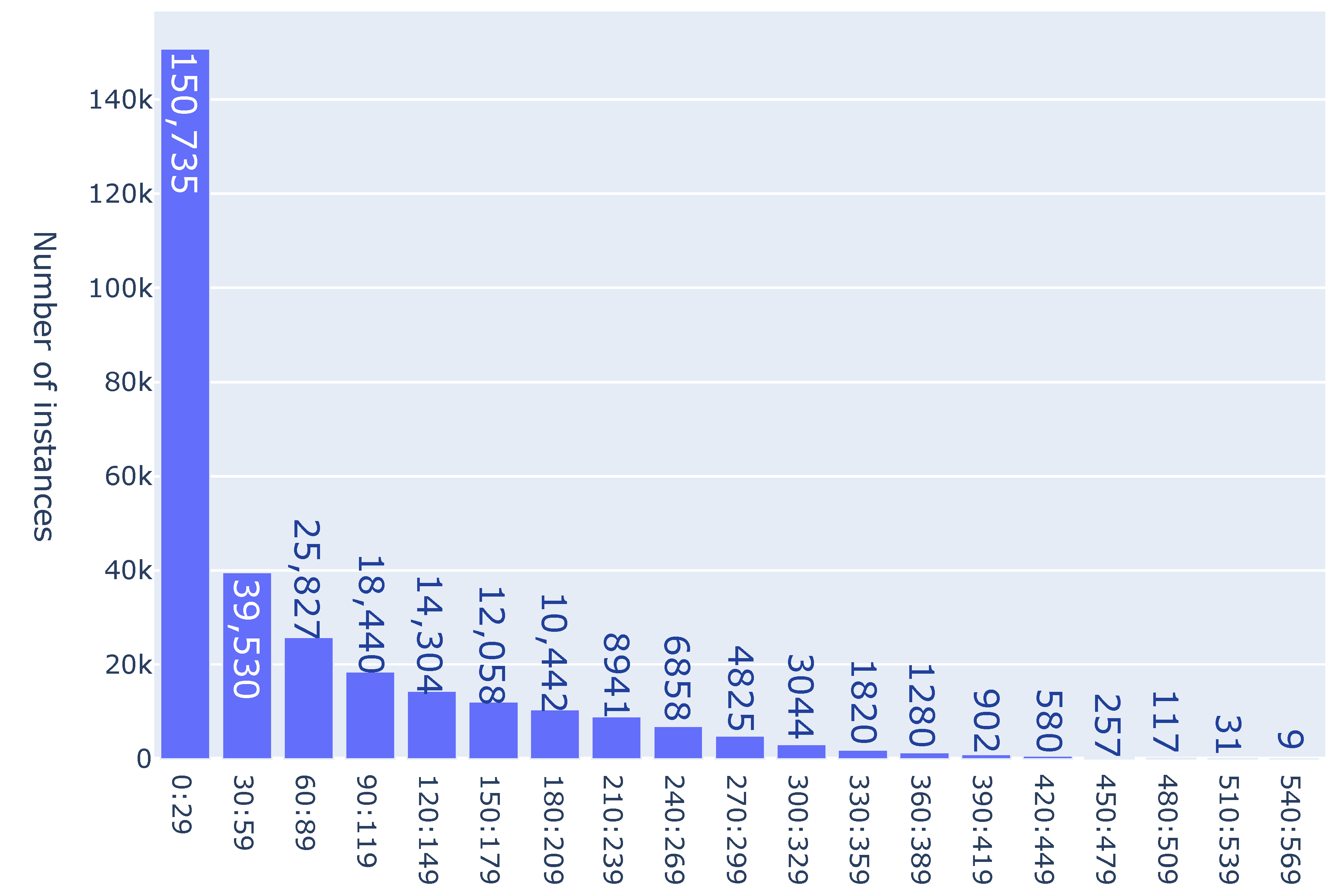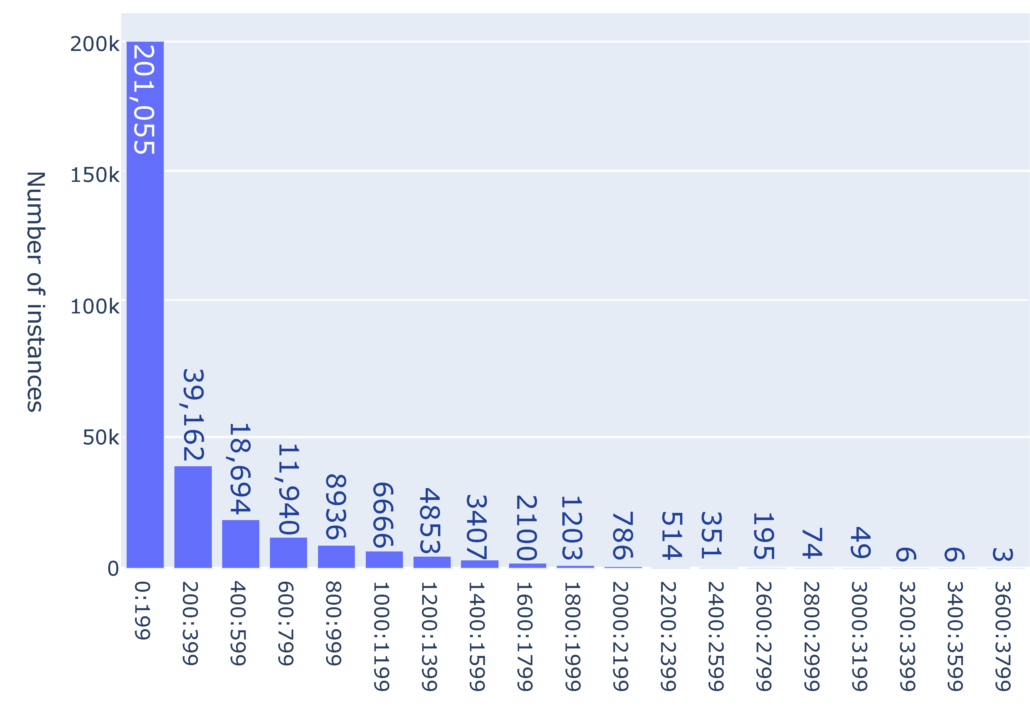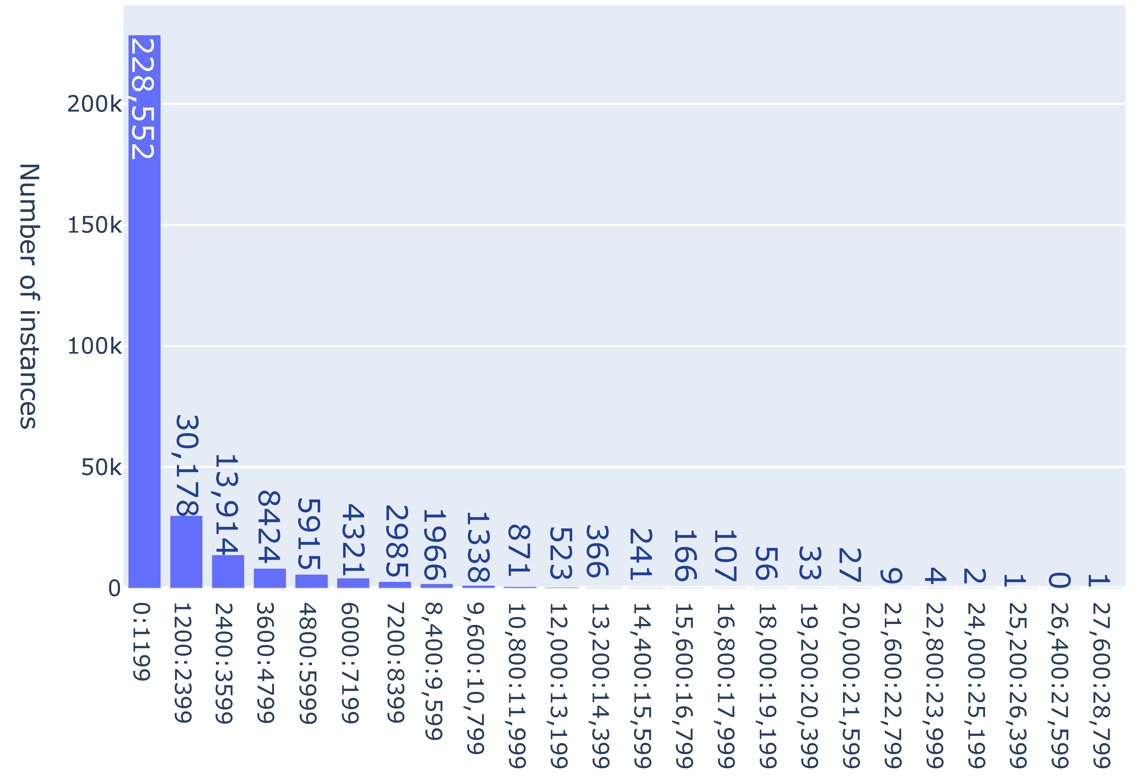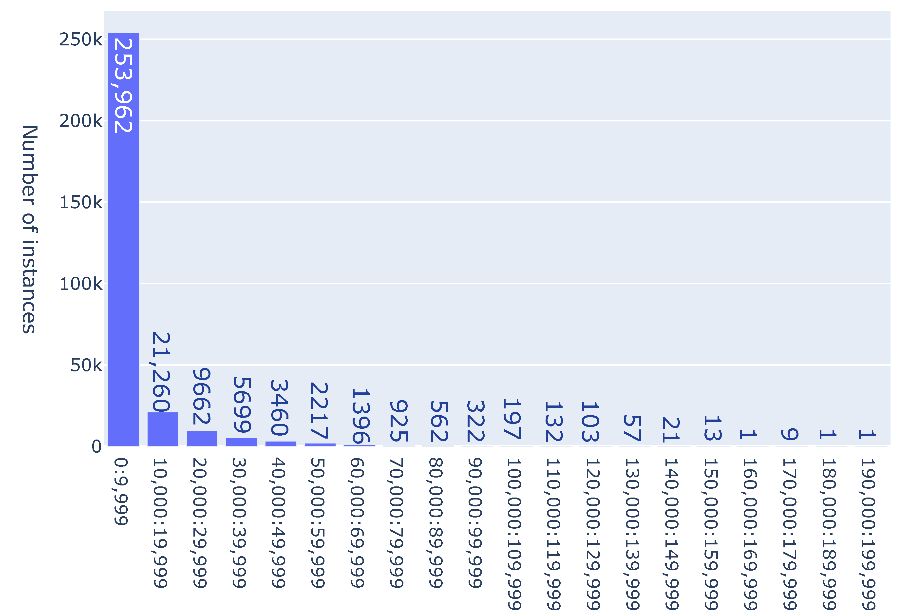Let the size of the cube be 100. We generated 300,000 points on the surface for problems with 4, 5, 6, 7, 8 and 9 jobs (i.e., in the 12-, 15-, 18-, 21, 24, 27-dimensional spaces, respectively). All instances have been solved, and we counted the number of iterations (i.e., branching points) for each problem instance. The results are shown in Figure 1 for the instances with 4 jobs, in Figure 2 for the instances with 5 jobs, in Figure 3 for the instances with 6 jobs, in Figure 4 for the instances with 7 jobs, in Figure 5 for the instances with 8 jobs and in Figure 6 for the instances with 9 jobs. 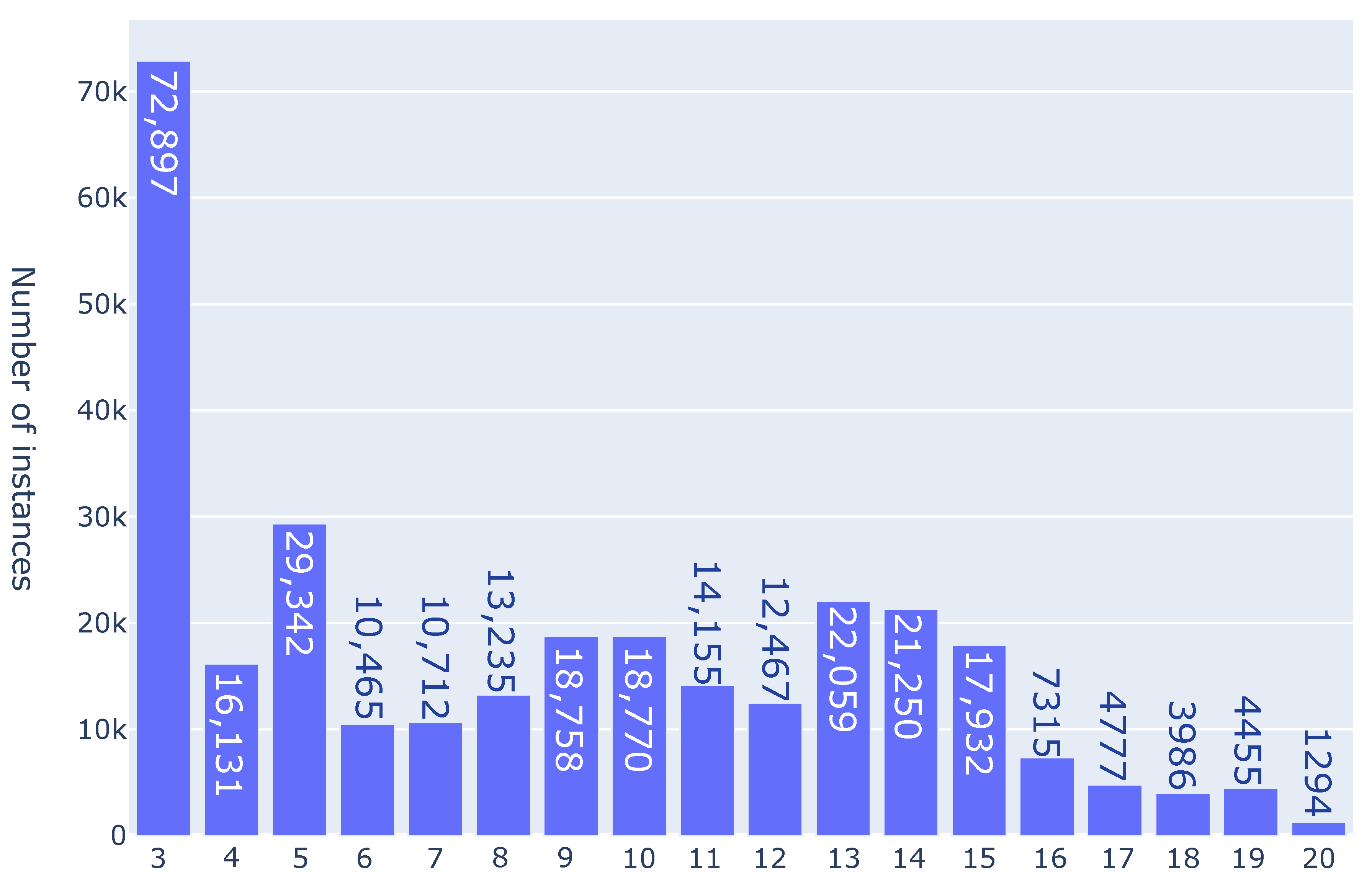At the y-axis, the numbers are given how often a particular number of branching points (Figure 1) or an interval for the number of branching points (Figure 2, Figure 3, Figure 4, Figure 5 and Figure 6) has occurred among the 300,000 instances for each number n of jobs. 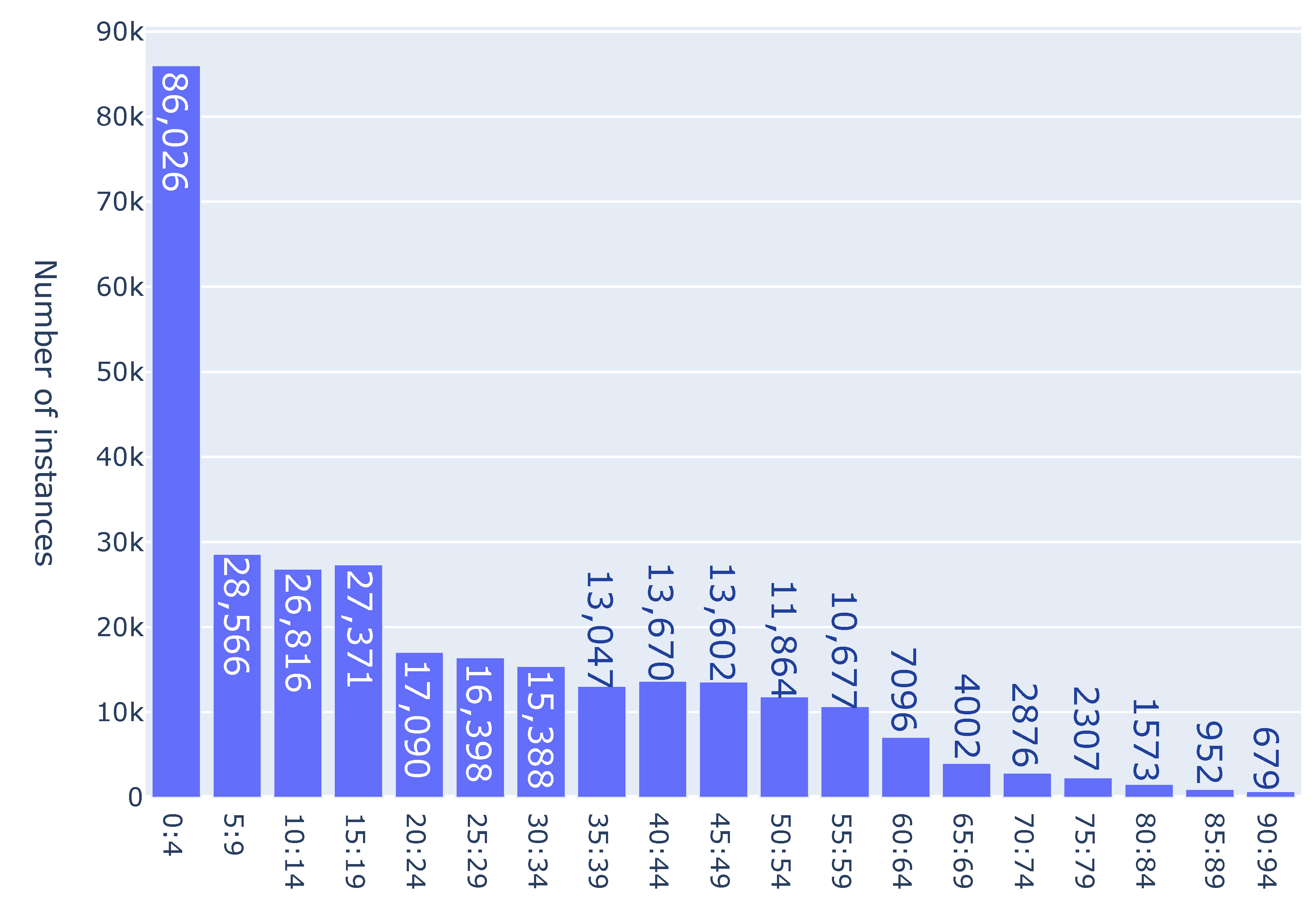For example, in Figure 1, one can see that among the 300,000 solved instances with 5 jobs, there were 72,897 instances with 3 branching points, 16,131 instances with 4 branching points, 29,342 instances with 5 branching points, and so on. It can be observed that the maximal number of 20 branching points was reached for 1294 instances, which is approximately equal to 0.4% of all instances. In Figure 2, the numbers of branching points are grouped in intervals of 5 in each column, i.e., there were 86 026 instances with several branching points between 0 and 4 (actually 4, because it is the minimum possible number of branching points for instances with 5 jobs), 28,566 instances with several branching points between 5 and 9, etc. For instances with 5 jobs, the maximum number of branching points was 93, and it was reached for only 33 instances. As it can be seen in the figures, most of instances can be solved by a small number of branches. For a larger number of jobs, one can detect a smaller number of hard instances with a large number of branching points. Thus, for the instances with 9 jobs, among the 300,000 solved instances, there were only two instances with several branching points more than 180,000: one with 184,868, and the other with 191,887.

5. Conclusions

For solving the $NP$-hard problem $1\mid r_j\mid {\phi }_{\max }$ for arbitrary non-decreasing penalty functions, an algorithm has been proposed which implements the branch and bound method. For each sub-instance to be considered, a lower bound on the optimal function value is determined using a solution of the dual problem. The proposed algorithm for solving the dual problem can find a solution in several operations not exceeding $O\left(n^2\right)$. The proposed algorithm can find an optimal solution within a time limit of one second for about 98% of the instances for 8 jobs and for about 85% of instances for 9 jobs. Although there are a few instances with a large number of branching points, most instances can be solved very fast by the proposed algorithm. For the hard instances, the execution of the algorithm can be interrupted at any moment, and the current objective function value with the corresponding schedule $\pi$ can be used as an approximate solution for the instance. However, some generated instances appeared to be very hard. At the moment, we cannot explain this interesting phenomenon. It requires deep additional investigations which are planned in the future.

In addition to the dual problem, the inverse problem has also been solved for the lateness objective function. The algorithm for solving the inverse problem has a complexity of $O\left(n^2\right)$ operations. However, in the problem of minimizing maximum lateness, one tries to ‘equalize’ the lateness while minimizing the maximum, in the inverse problem the lateness values are ‘equalized’ due to the maximization of the minimum provided that inserted machine idle times are prohibited.